Effect of Mimic Vegetation with Different Stiffness on Regular Wave Propagation and Turbulence

1
Guangdong Research Institute of Water Resources and Hydropower, Guangzhou 510630, China
2
School of Marine Sciences, Sun Yat-sen University, Guangzhou 518000, China
*
Author to whom correspondence should be addressed.
Water 2019, 11(1), 109; https://doi.org/10.3390/w11010109
Submission received: 28 September 2018
/
Revised: 25 December 2018
/
Accepted: 29 December 2018
/
Published: 10 January 2019
(This article belongs to the Special Issue Coastal Vulnerability and Mitigation Strategies: From Monitoring to Applied Research
)
Abstract
:Flume experiments were performed to test four plant mimics with different stiffness to reveal the effect of plant stiffness on the wave dissipation and turbulence process. The mimics were built of silica gel rod groups, and their bending elastic modulus was measured as a proxy for stiffness. The regular wave velocity distribution, turbulence characteristics, and wave dissipation effect of different groups were studied in a flume experiment. Results show that, when a wave ran through the flexible rod groups, the velocity period changed gradually from unimodal to bimodal, and the secondary wave peak was more apparent in the more flexible mimics. The change in the turbulence intensity in the different rod groups showed that the higher the rod stiffness, the greater the turbulence intensity. With an increase in the bending elastic modulus of a rod group, the wave dissipation coefficient increased. The increase in the wave dissipation coefficient was not linearly correlated with the bending elastic modulus, but it was sensitive within a certain range of the elastic modulus.
1. Introduction
Waves are one of the most important hydrodynamic force in coastal environments [1,2,3]. The reduction of coastal erosion induced by waves is an important topic for coastal protection and morphological changes [4,5,6]. Plants, such as mangroves, play an important role in protecting coasts. The planting of forests for wave attenuation in front of seawalls can reduce the arrival of waves, reduce the impact force of waves, and enhance the security of dams. It is known that different plant properties (e.g., density, stiffness, flexibility, arrangement mode, degree of submergence, and other factors) produce different influences on momentum transfer and the turbulence structure in canopy flow [7,8,9,10,11,12]. These related processes can lead to different sediment deposition patterns, which can influence the coastal morphology. The interesting point is that even the presence of a short, low-biomass seagrass meadow can lower the beach erosion rates compared to shallow unvegetated nearshore reef flats [13,14,15,16]. However, wave interactions between plants with varied stiffness have not been fully understood.
To investigate these interactions, Huang et al. [17] designed a physical model with a rigid main trunk and flexible branches and leaves. They then systematically analyzed wave propagation behaviors on a vegetated floodplain, as well as the effect of plant branches and leaves, tree trunks, the width of the beach, the depth of the water on the beach land, and wave elements on the propagation and deformation of the wave. Jiang et al. [18] used a physical model experiment of a wave flume to study the effect of changes in the wave height and wave form. Incident wave height, plant densities, reflection, transmission coefficient, and the wave energy dissipation were investigated. Moller and Spencer discovered that wave height decreased exponentially in a vegetated area [19]. Quartel et al. [20] performed an experiment at the Red River Delta in Vietnam and found that the wave dissipation ability of mangrove areas is five to 7.5 times more than that produced due to bottom friction. Bradley and Houser [21] quantitatively analyzed the effect of the relative movement of flexible seaweed leaves on wave height reduction in a reversing current. Fonseca and Cahalan [22] and Augustin et al. [11] showed that, when the height of seaweed was greater than or close to the water depth, the wave dissipation effect was obvious, and when the plant was submerged, the wave dissipation effect decreased with increased water depth. Tschirky and Hall [23] and Lima et al. [24] performed experiments that indicated that an increase in plant density enhanced the wave dissipation effect. However, Mazda et al. [25] and Horstman et al. [26] found that when the water depth in the mangrove was more than the height of the aerial roots, an increase in water depth reduced the wave dissipation effect, and when the water depth increased to the height of the mangrove leaves, the wave dissipation effect increased. Cruise and Muslesh [27] used a rigid pole to simulate the emerged portion of rigid vegetation and studied the effect of plant diameter and arrangement on water depth and velocity. White and Nepf [28] also studied the plant drag force, flow turbulence, and diffusion with a rigid rod.
Currently, there are many laboratory studies on vegetation under unidirectional currents and/or waves [29,30,31,32], field studies on wave dissipation through flexible vegetation [33,34,35,36], and turbulent flow through real mangrove roots [37]. However, the wave propagation and turbulence in vegetation with different stiffness is currently less studied [8].Therefore, in this study, the main aim is to study the wave propagation and turbulence characteristics among vegetation with different stiffness. A type of mimics used in this study is completely rigid, and the other three types of mimics are flexible to mimic the stems of macro algaes like Fucus vesiculosus and Fucus serratus with comparable elastic modulus (0.121–0.585 Gpa) [38]. The bending elastic modulus were measured using plant mimics made of silica gel rods with different stiffness. The regular wave velocity distribution, turbulence characteristics, and wave dissipation effect of different groups were studied to better understand the wave dissipation process through a vegetated field. The knowledge obtained by this study may provide a scientific reference for the planning and design of coastal protection projects.
2. Experimental Setup
2.1. Experimental Design
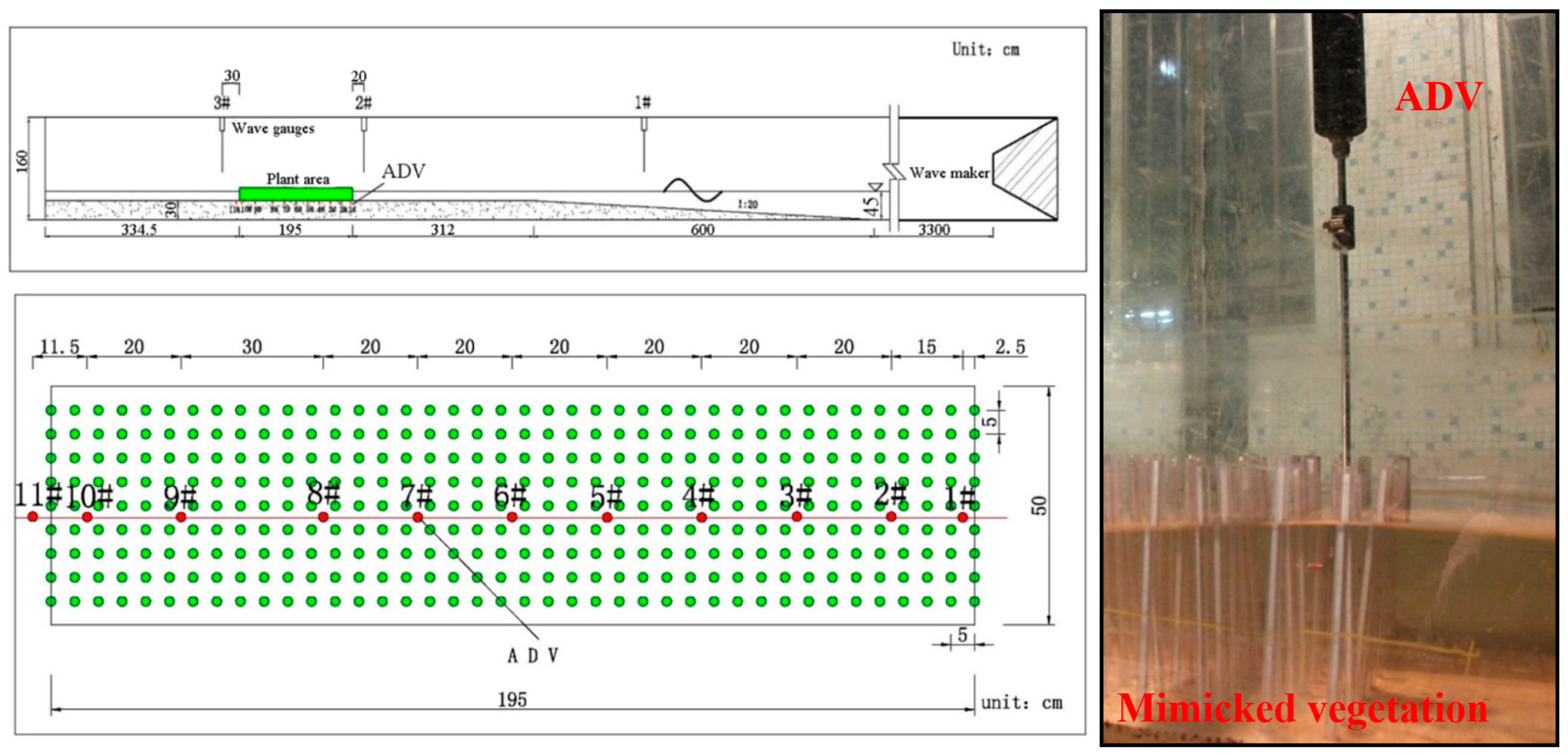
Experiments were conducted in a laboratory wave flume. The dimensions of the flume were 66 m long, 1.0 m wide, and 1.6 m deep. A piston-type waves paddle installed at one end of the flume was used to generate regular and irregular waves. For simplicity, we only tested regular waves in the current study. An overview of the flume, with its coordinate system and the wave maker, is shown in Figure 1. All of the instruments were deployed in this flume. Details of the flume dimensions and sensor deployments are also shown in Figure 1. The water surface elevation was measured using capacitance-type wave probes with good long-term stability and linear calibration curves. The wave probes were calibrated just prior to conducting the experiments. A SonTek 16-MHz Micro ADV (Acoustic Doppler Velocimeter) (SonTek/Xylem Inc.: San Diego, CA, USA) was used to measure the three-dimensional water velocity. The sampling frequency of the ADV and wave gages is 50 Hz. The data were collected after the waveform stabilized in the front of the mimic vegetation area, and the data collection lasted for 60 s. In order to eliminate the error, each experiment was repeated for three times. Peak velocities were obtained by taking the maximum value of an entire wave period.
The vegetation zone was composed of silica gel rods of different stiffness installed on a flat slope. The rods were fixed though the prefabricated holes on the at the slope bed. Wave gauges were installed before and after the vegetation zone to quantitatively measure the wave attenuation. The 3D flow field structure and turbulence characteristics were measured using the ADV. The current velocity was measured at the middle and bottom layers at 10 cm and 2 cm above the bed using the ADV. These two measuring points are regarded as representative heights of the vertical profile, while the information of the whole profile was not obtained.
The wave and flow design included no wave breaking action nor the presence of emergent vegetation. Therefore, the designed water depth of the floodplain was 15 cm, and the corresponding water depth before the wave plate was 45 cm. In addition, the regular wave height was 5 cm, and the wave period was 1.34 s. The resulting wave length was 1.53 m, and the tested water depth (0.15 m) in the vegetation canopy was half water depth. The wave condition is similar to previous lab work with small waves (wave height H ≤7 cm) [36,39].
2.2. Experiment Materials
The diameter of plant mimics (d) was 1 cm and mimic height (hv) was 20 cm, and they were arranged into a rectangle with a total width of 195 cm consisting of 40 rows that were 5 cm apart with columns 5 cm apart (See Figure 1). The height of the mimics was determined to be similar to F. vesiculosus. The projecting area was 289.85 cm2, which is also similar to the field conditions of F. vesiculosus [38]. Thus, essentially, this experiment did not involve scaling, as the tested mimics were dynamically similar to F. vesiculosus in the field conditions and the tested wave condition was also similar to the real field condition (depth = 0.15 m, wave height = 0.05 m, and period = 1.34 s). In the current experiment, the tested Re (Re = u × d/ν, where u is the velocity of the middle and bottom layers) number range was generally between 1000 and 2000.
Eleven measuring point was set along the center-line of the wave flume to minimize the influence of the side-wall. The obtained velocities and turbulence statistics are regarded as the representative measurements of the flume cross section. However, pair ADV measurements in the lateral direction were not conducted in our experiment. Thus, the current study mostly focused on velocity in the streamwise direction, i.e., u. The u velocity is positive when it is in the same direction as wave propagation, and it is negative when it is opposite to wave propagation.
We used a spring scale for the cantilever measurement. 10 rods of the same material were involved in each test and the experimental results are averaged. The elasticity modulus was calculated using the cantilever beam formula, and the stiffnesses of different materials were measured as:
where E is the elasticity modulus (Pa); u is the offset distance (m); F is the transverse tensile force (N); I is the inertia moment, i.e., I = πd4/64 for a circle; and L is the rod length (m).
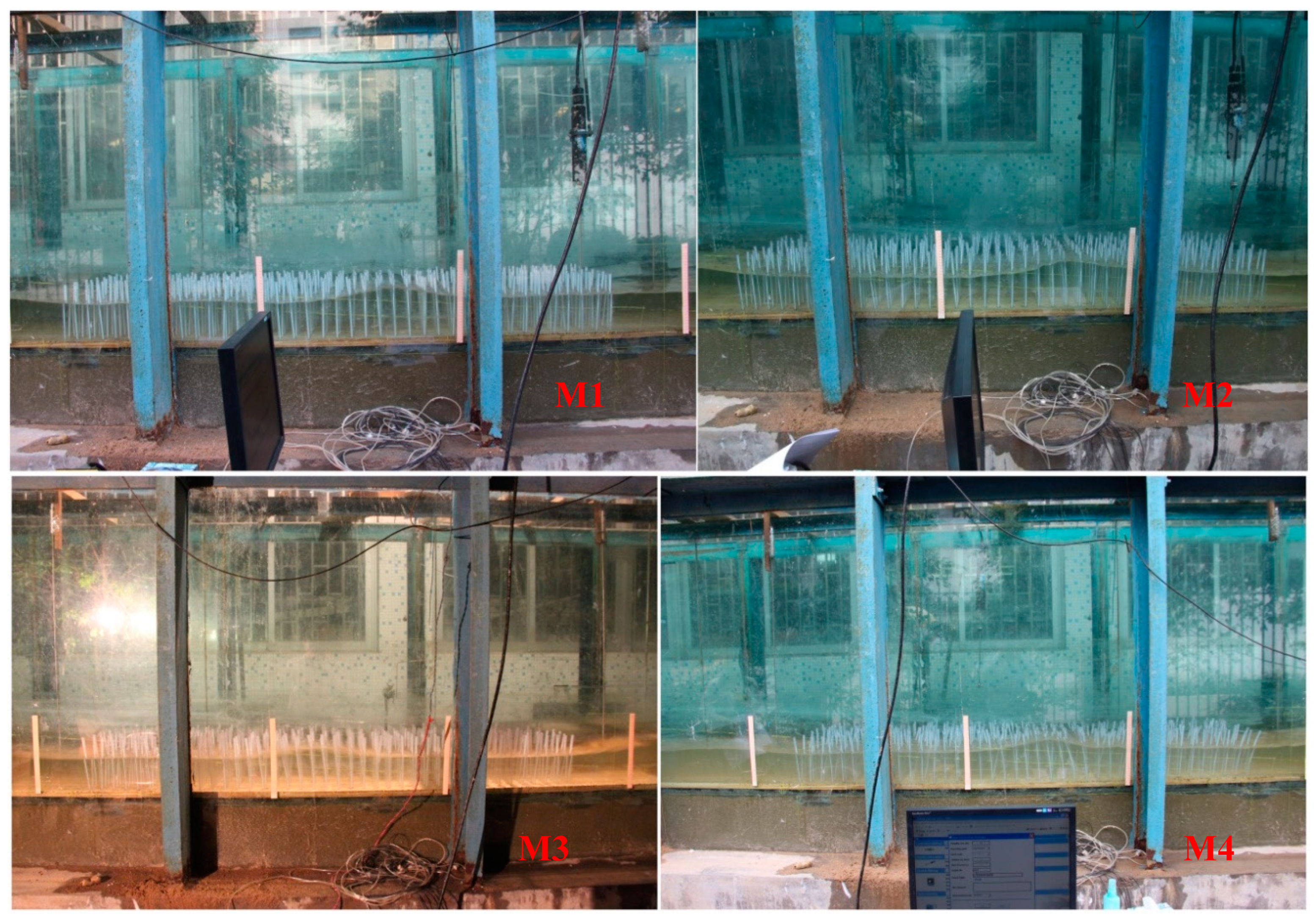
The elastic modulus of the rods is shown in Table 1. Materials 1, 2, 3, and 4 with different stiffnesses are denoted as M1, M2, M3, and M4, respectively (Figure 2). These rods were commercially available. The elastic modulus of M1 was significantly greater than the others, and it was able to keep upright throughout the entire process. Therefore, M1 can be seen as a rigid rod.
2.3. Data Processing
The original data were phase-averaged according to Cox’s theory [40]:
On the basis of points, the original 3D data were divided into three directions and circles. Using the phase average, the velocity of each point in one circle can be obtained, and the fluctuating velocity can be presented as follows:
Turbulence intensity is the root mean square of the fluctuating velocity:
The probability density function of random data means the probability of an instantaneous value being within a specified range. For the turbulent process, the probability of its value, u(t), being in the can be defined as the following:
where is the measuring time; and is the sampling time within , . A probability density function of velocity measurements was made for each material. If this random process is a normal distribution, then the probability density function can be found using the following equation:
where is the probability density; and is the fluctuating velocity in the direction.
Reynolds stress is the shear force caused by the momentum exchange of a unit fluid passing through a unit area. The equation is the following:
where when , , and is the normal stress; when is the Reynolds shear stress.
3. Results and Discussion
3.1. Velocity Variations in the Mimicked Vegetation Canopy with Different Stiffnesses
3.1.1. Peak Velocities
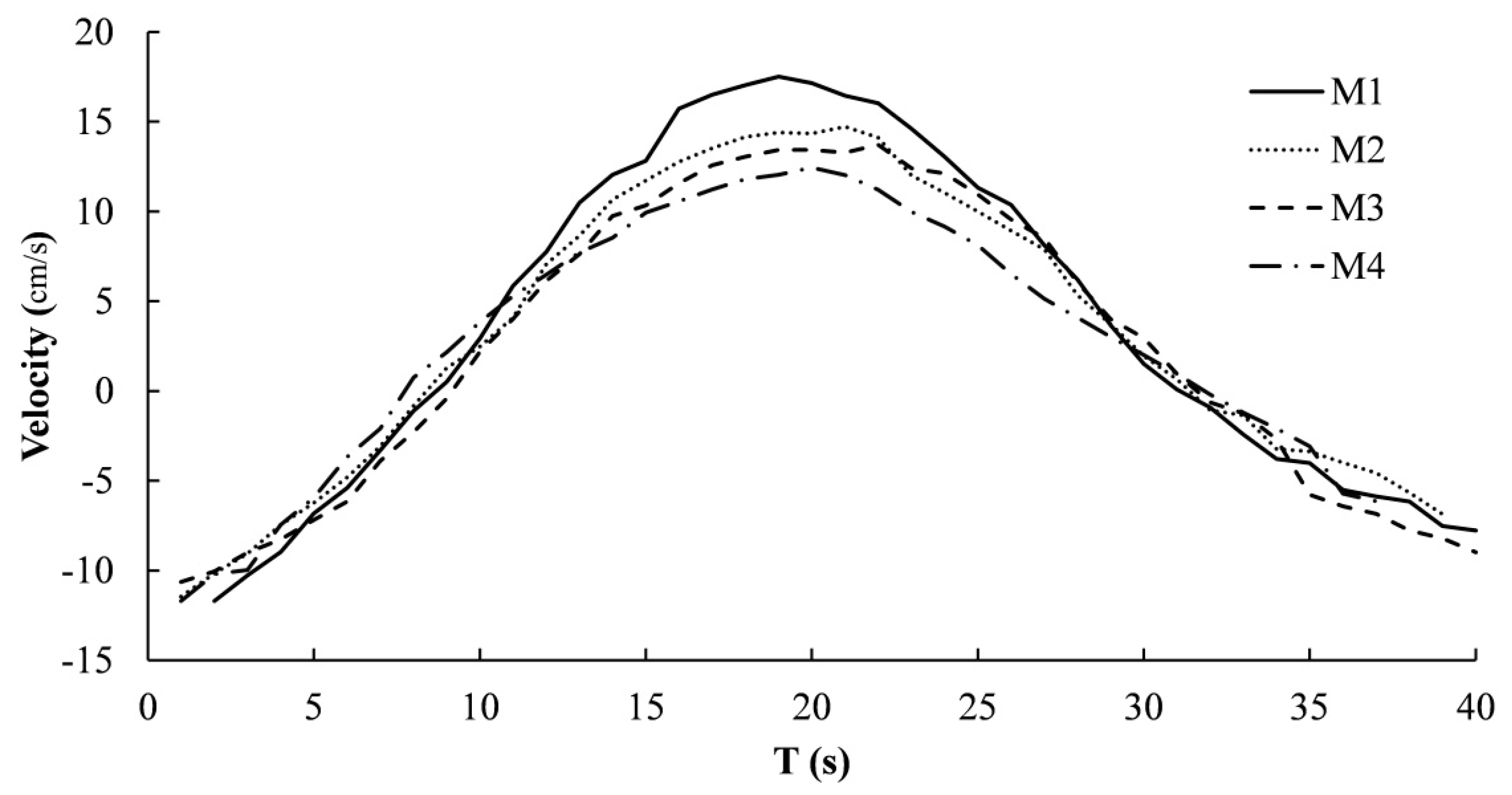
The peak velocities changed significantly when waves crossed the different rod groups. The more flexible the plant, the smaller the peak the velocity. Table 1 shows the value of the velocity peaks. It was found that with an increase in rod flexibility (from M1 to M4), the velocity peak value in the middle and bottom layer both gradually diminished. Compared to M1, the peak value of the middle and bottom layer of M4 were reduced by 31% and 32%, respectively. The peak velocity value between two rods was increased. It is because rigid rods do not have any swing deformation, which squeezes the passing water and leads to higher velocity. For flexible rods, however, they sway as water passes, and hence do not lead to similar increased velocity. In fact, as the flexibility increases, the averaged velocity reduces (Figure 3).
Flexible rods do not cause contraction of the flow passing the flume section because of the unsynchronized swing. Therefore, the peak wave velocity was small. This is similar to what occurs when a bridge makes a channel narrow and increases the flow velocity.
3.1.2. Phase Averaged Velocity
According to the instantaneous velocity measured using the ADV, phase velocities in the direction of u are shown for different rod groups in Figure 3. Data from measuring point #5 is shown as it is in the center of the vegetation patch and it is representative of the averaged flow condition. The velocity curve shows that with a phase shift, the more flexible the materials are, the lower peak flow is. With a low flow velocity, the differences among the flow velocities of different materials are not obvious.
3.1.3. The Secondary Wave Peak in the Flexible Rod Groups
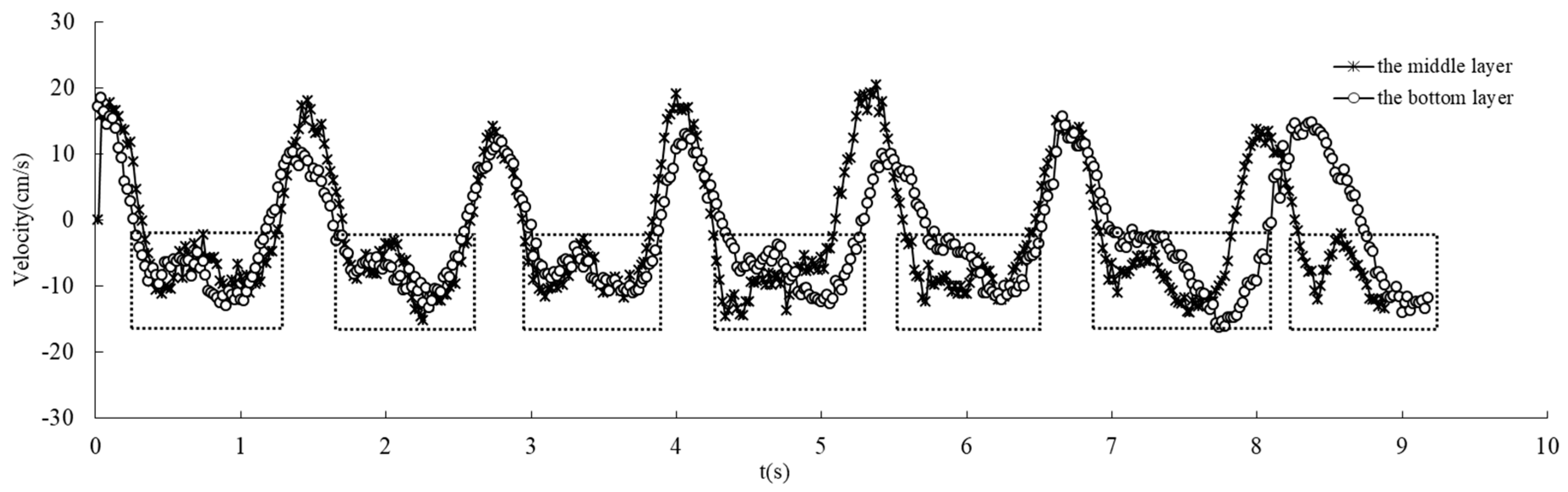
The experimental results show that when waves went through the flexible rod groups, the velocity period changed gradually from unimodal to bimodal, owing to swing in the rod group. The more flexible the rod group, the more obvious the secondary wave peak. Figure 4 shows velocity of the M4 rod group at measuring point #5. The figure shows that both in the middle and the bottom layer, bimodal structures existed during each wave period. The ratio between the secondary wave peak and the main wave peak in the middle layer was 0.49:1, while in the bottom layer it was 0.31:1. This phenomenon indicates that the swing extent of a rod increases as the water surface approaches, and its impact on the secondary peak of the wave velocity also increases.
3.2. Turbulence Characteristics of the Different Rod Groups
3.2.1. Turbulence Intensity
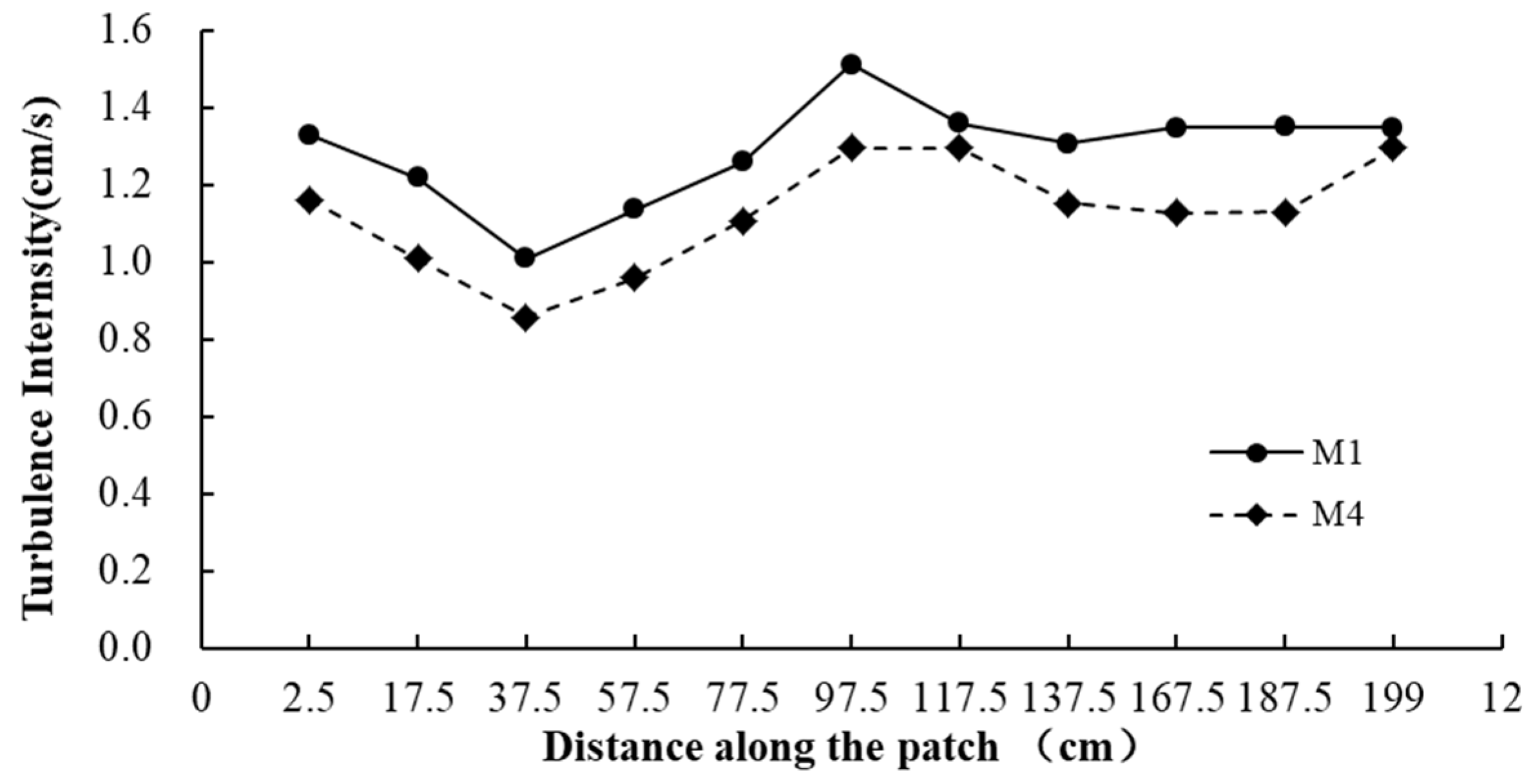
The middle layer turbulence intensity distributions in the u direction for the M1 and M4 rod groups are presented in Figure 5. The middle and bottom layer turbulence distributions of the different materials are shown in Figure 6. Spatial changes in the turbulence intensity indicates that the highest value occurs during the period of the wave entrance into the rod group and in the middle of the rod group. Possible explanations include the following: (1) The water’s entrance into the rod group means that the wave propagates from one interface to another interface, which can result in intense turbulence; and (2) wave streaming causes intense turbulence when the wave propagates in the middle of the rod group.
The turbulence intensity changes in different materials indicate that the greater the material stiffness, the stronger the turbulence velocity and intensity. From M1 to M4, the turbulence intensity reduces 5.1%, 5.4%, and 4.4%, respectively, in the u direction of measuring point #5. This result is similar to that of a previous experiment by Pujol et al., [29].
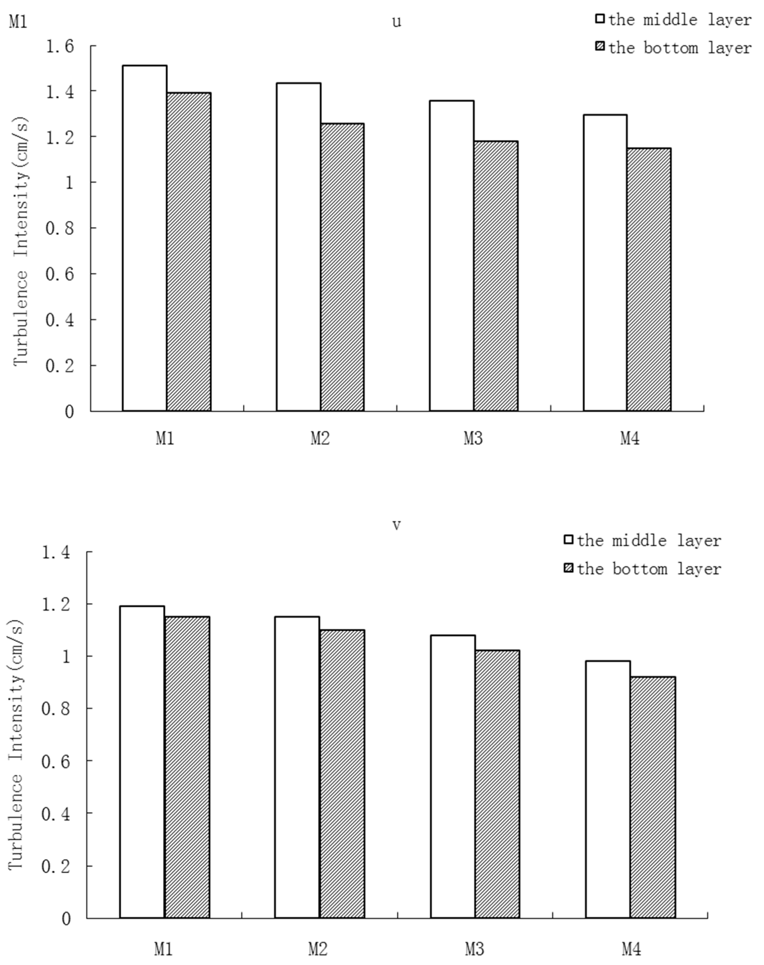
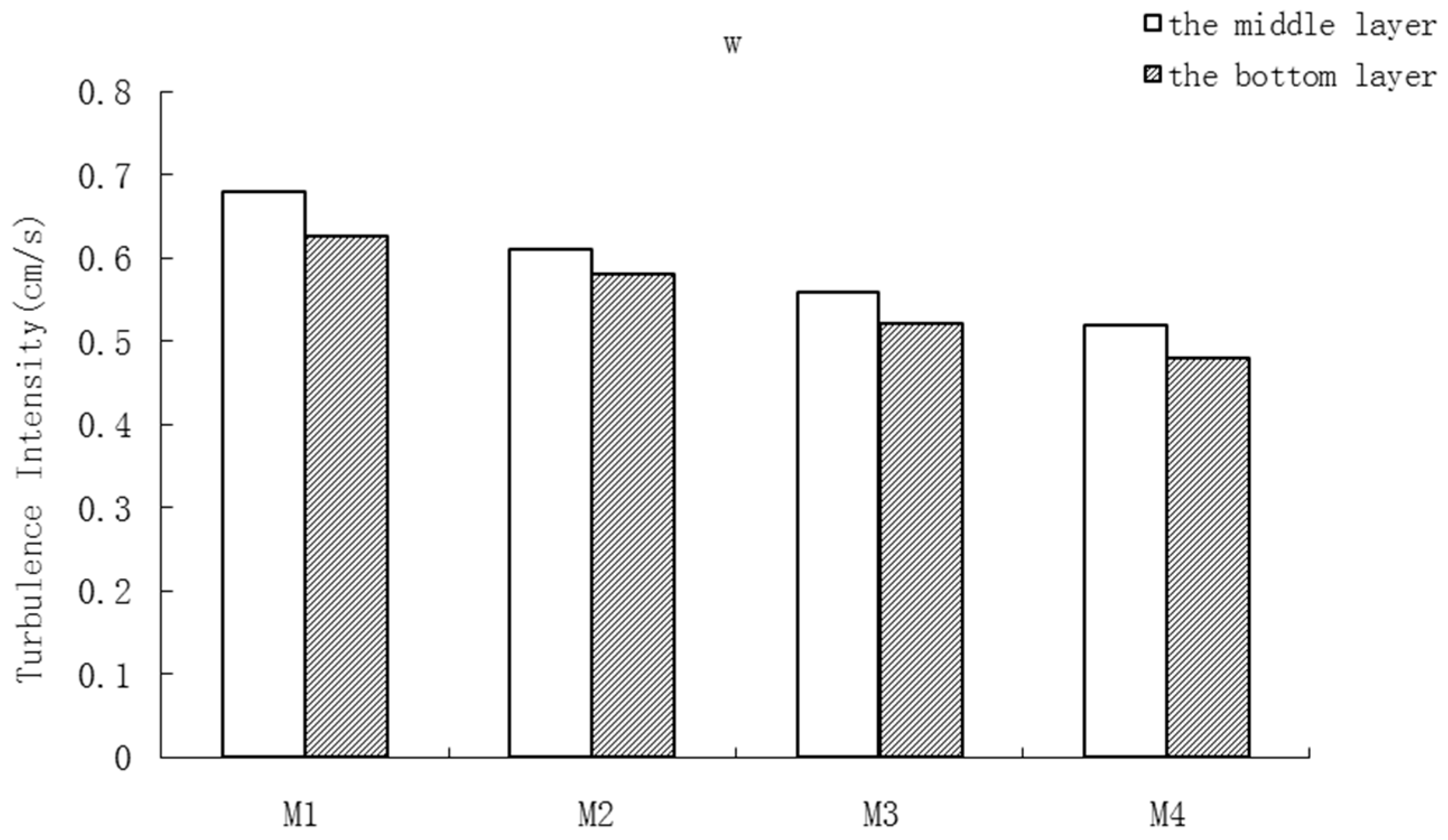
The turbulence intensity in different directions shows that the largest was in the u direction followed by the v direction, and the intensity in the w direction was minimal. As far as the vertical distribution, the turbulence intensity in the bottom layer was smaller than in the surface layer. This reflects that turbulence was anisotropic when the vegetation patch was under wavy flows.
3.2.2. Probability Density of the Fluctuating Velocity
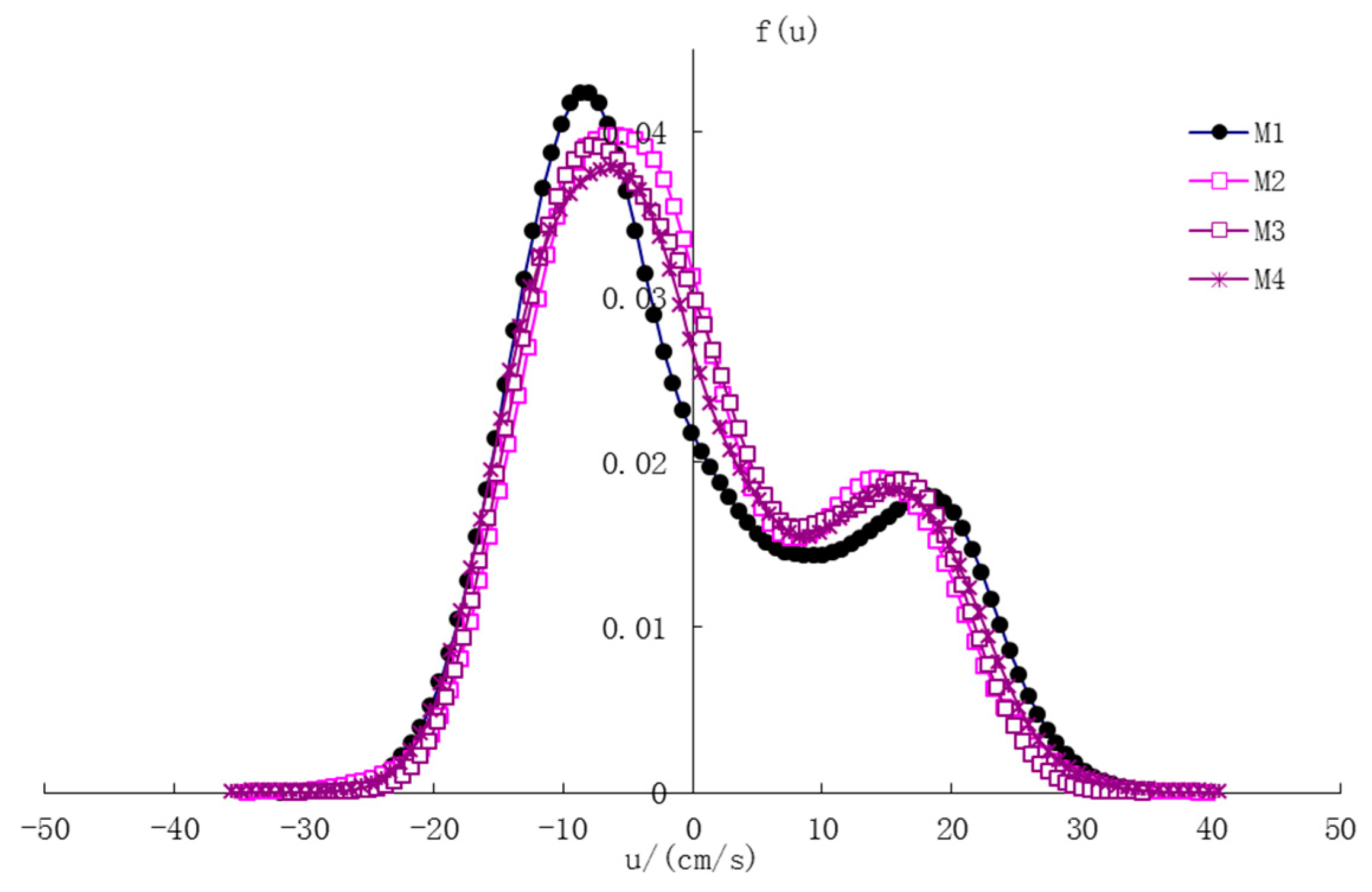
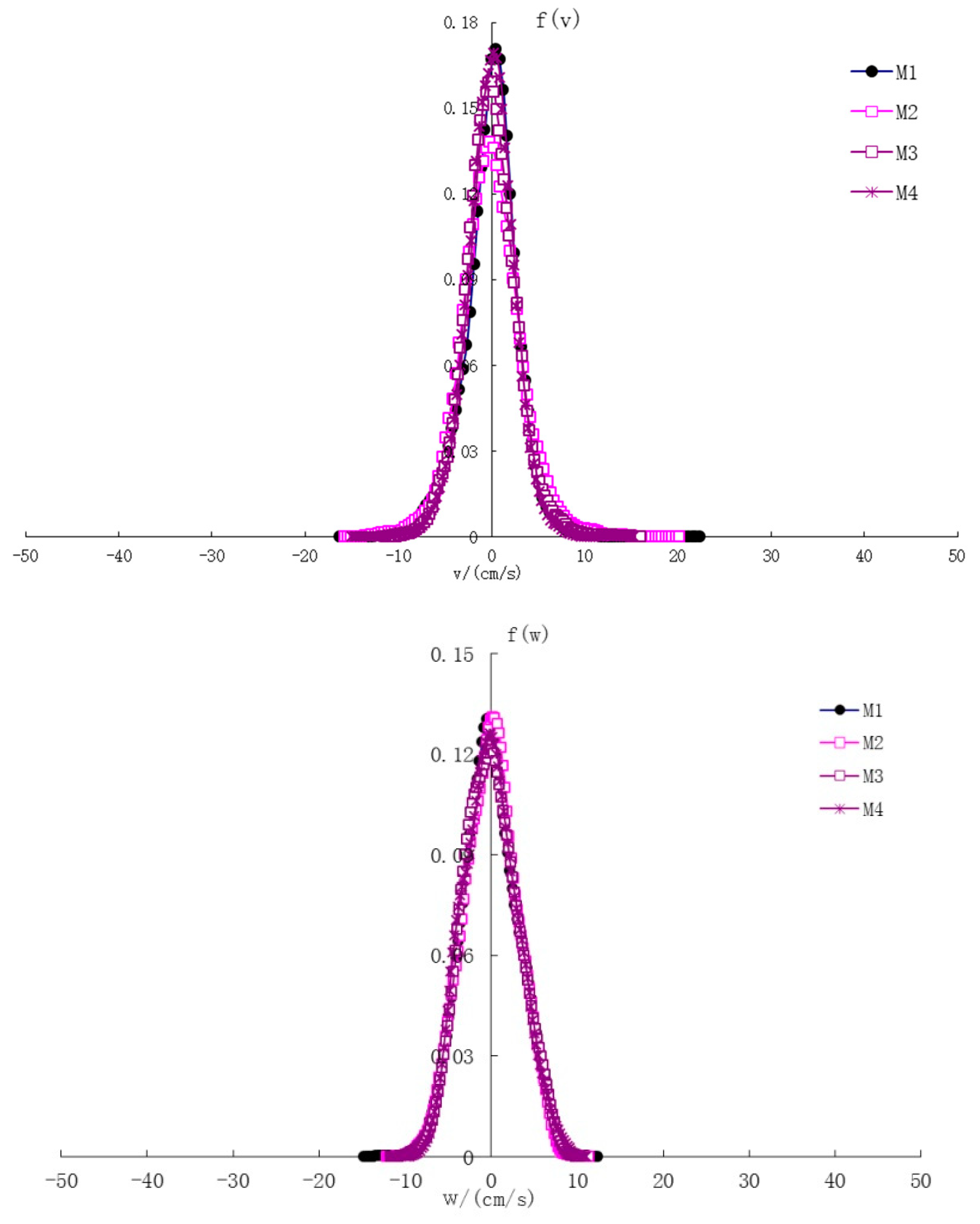
If the probability density is a normal distribution, the wider the graph, the larger the velocity deviation. The y axis intercept is the turbulence intensity in Figure 7. Figure 7 shows the probability density distribution of the fluctuating velocity in the , and directions. Two peak values are found in the probability density function of the direction, and at the same time, the turbulence intensity decreases with an increase in the flexibility of the rod group. While in the direction and direction, the probability density follows a normal distribution, and the differences between different materials are not obvious.
3.2.3. Reynolds Stress
Reynolds stress is generally greater than the viscous shear force in vegetated flows [41]. Therefore, only near the sidewall is the viscosity term considered, otherwise it is ignored.
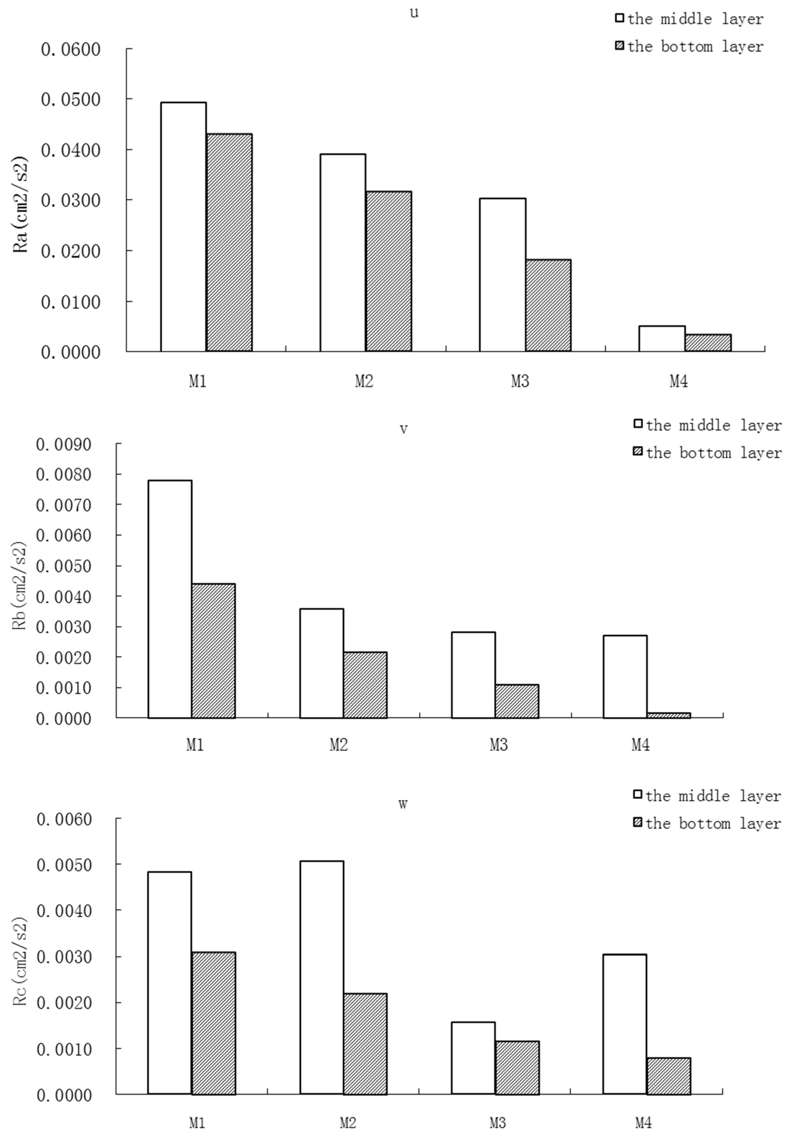
Reynolds stress is the result of an uneven flow velocity distribution in a flow field. Therefore, the more uneven the velocity distribution is, the greater the Reynolds stress is, and the stronger the turbulence. Figure 8 shows the change in Reynolds stress for different rod groups, where , and (, , and represent fluctuating velocities in the , , and directions, respectively). Results show that the Reynolds stress decreases with increasing stiffness. The Reynolds stress of the M4 middle layer is only 10% that of M1.
Moreover, the Reynolds stress of the middle layer is larger than the bottom layer, which is similar to Ma’s [42] research on the wave turbulence. The middle layer Reynolds stress is about 1.14 times that of the bottom layer in the rigid rod group (M1), and about 1.52 times that of the flexible rod group (M4).
3.2.4. Energy Spectrum Density
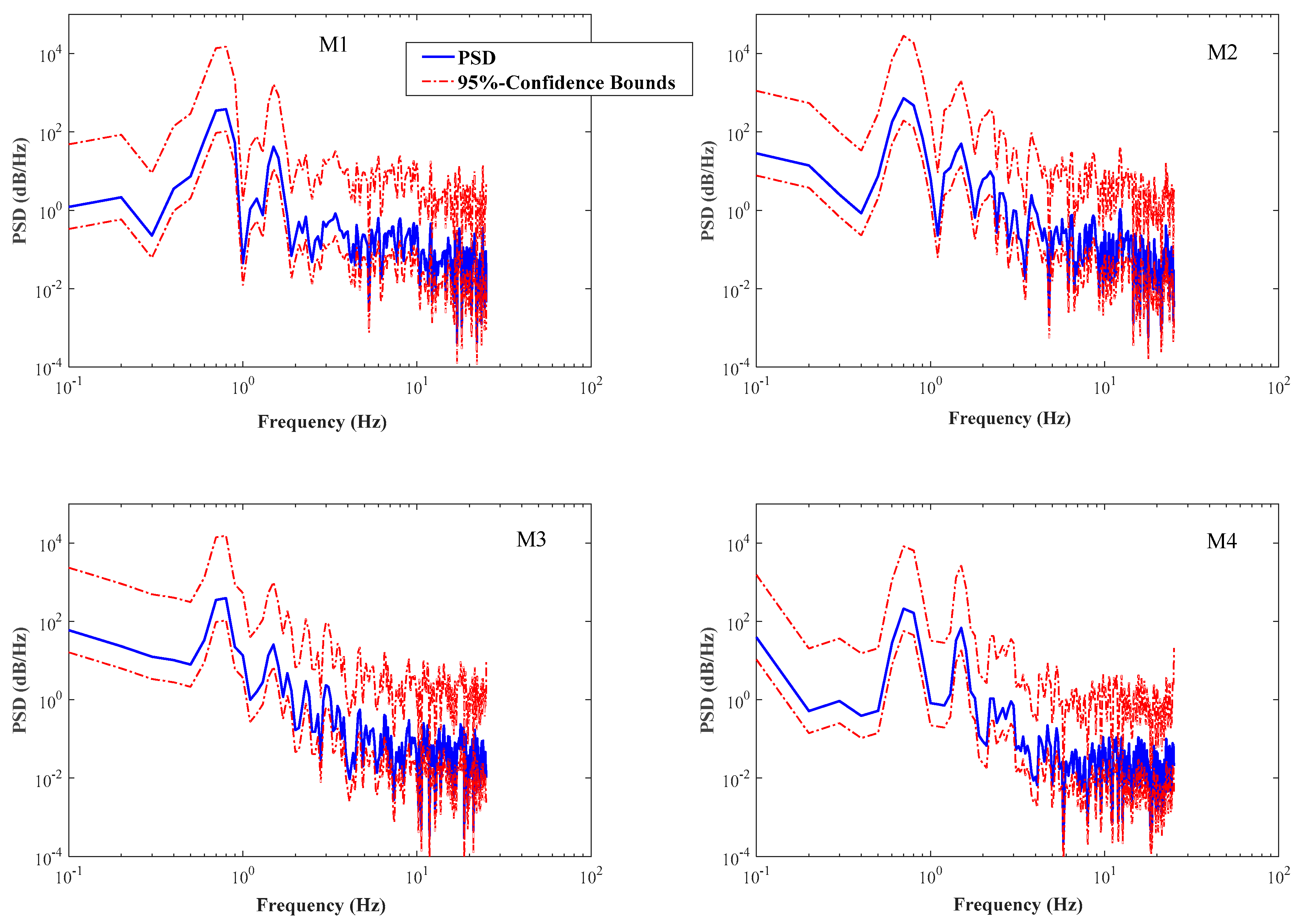
The turbulent process can be seen as superposition of simple harmonic waves with different frequencies. Velocity spectra were computed and give the parameters used to compute the power spectra (E(n), ). The energy spectral density curve represents the distribution of turbulent kinetic energy in a wave band in steady time. Time is the inverse of frequency. We set a 95% confidence interval on each of the spectra to eliminate the effect of noise. The high frequency in the energy spectrum represents the quickly changing turbulence, or turbulence on a small time scale [43].
The energy spectral density distributions in the u direction for different material rod groups at measuring point #5 are shown in Figure 9, which is related to the wave energy transmission process. As can be seen from the figure, when a wave propagates in the rod groups, two energy spectral peaks exist, with the main peak value larger than the secondary peak. With a reduction in material rigidity, the main peak value of the wave energy decreases, which means that the wave turbulence intensity is reduced. Furthermore, the secondary peak of M4 is the largest among all the cases. The secondary peaks were related to rod group swing. The more flexible the rod group was, the more obvious the secondary wave peak was.
3.3. Wave Dissipation Effect in the Different Rod Groups
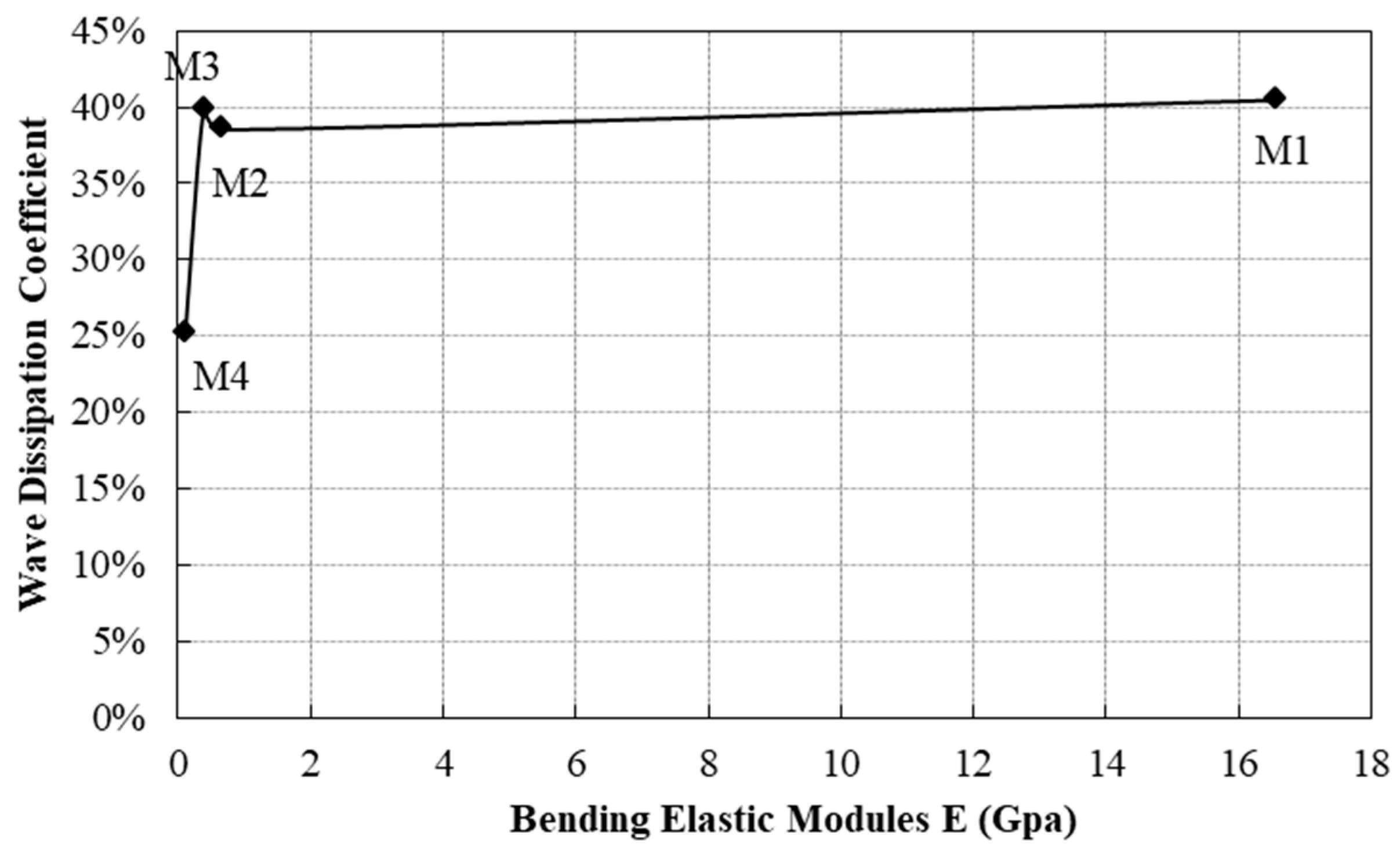
The change in wave height before and after the wave moves through the rod groups represent the attenuation of wave energy (see Table 2 and Figure 10). When the bending elastic modulus of the rod group increases from 0.11 GPa to 0.39 Gpa (Compare M4 with M3), the wave dissipation coefficient correspondingly increases from 25.17% to 39.79%. When the flexural elastic modulus increases from 0.39 GPa to 16.56 Gpa (Compare M3 with M1), the wave dissipation coefficient increases from 39.79% to 40.45%, only an increase of 1.66%. M2 and M3 may have happened to be in an area that was insensitive to stiffness, causing the wave dissipation coefficients to fluctuate.
Overall, the wave dissipation coefficient increases with increases in the bending modulus of elasticity in the rod group. More succinctly, the greater the stiffness of the rod group is, the more obvious the energy dissipation effects will be. In addition, the growth of the wave dissipation coefficient is not linear with the bending elastic modulus; but is sensitive within a certain range of the elastic modulus. There is a sharp quick increase in the wave dissipation coefficient. However, when the bending elastic modulus value increases to 0.39 Gpa, the wave dissipation coefficient growth becomes extremely small.
The above behaviors can also be interpreted from the physical phenomenon point of view. M3 and M4 obviously swing more under wave flow. M2 only slightly swings when the wave peak passes. M1 is completely rigid and does not swing. This phenomenon shows that the bending elastic modulus values of M3 and M4 happen to be in the most sensitive ranges for a swing reaction under group wave conditions; that is, in the most sensitive ranges for a change in the wave dissipation coefficient.
Our results showed that when waves ran through flexible vegetation mimics, the velocity period changed gradually from unimodal to bimodal. This phenomenon is likely due to the swaying effect of the flexible vegetation [8,31], as it is more apparent with flexible mimics. The change in the turbulence intensity in the different rod groups showed that the higher the rod stiffness, the greater the turbulence intensity exists. This result is similar to that in Reference [29]. With an increase in the bending elastic modulus of a rod group, the wave dissipation coefficient increased, which is consistent with the previous studies [39,41]. However, the increase in the wave dissipation coefficient was not linearly correlated with the bending elastic modulus. It was more sensitive in a certain range of the elastic modulus than others.
4. Conclusions
The bending elastic modulus was measured using a conceptual plant model that was built of silica gel rod groups of different stiffness. The regular wave velocity distribution, turbulence characteristics, and wave dissipation effect of the different groups were studied. According to the results, the conclusions that follow can be drawn.
- (1)
- When waves went through different material rod groups, the peak velocity of the wave was in decay. The more flexible the rod group, the smaller the peak flow velocity. With a low flow velocity, the differences among the flow velocities of the different materials was not apparent.
- (2)
- When waves go through the flexible rod group, the velocity period gradually changed from unimodal to bimodal. Owing to rod group swing, the more flexible the rod group was, the more obvious the secondary wave peak was. With a reduction in material rigidity, the second peak value of the wave energy decreased, which was related to flow shocks that were caused by the swing of the flexible rod group. It is expected that, with different wave periods, the swing behavior and the wave energy transmission will be different, which should be further studied.
- (3)
- High turbulence intensity existed in the areas at the front and in the middle of the rod group. This was because when the wave entered the rod group, the wave propagated from one interface to another, resulting in intensified turbulence.
- (4)
- The greater the material stiffness was, the stronger the turbulence velocity and intensity were. The Reynolds stress decreased with increased flexibility. Additionally, the middle layer Reynolds stress was generally larger than that at the bottom layer.
The insights on different patterns in wave propagation turbulence intensity in different canopies may lead to further understanding of the coastal morphological changes with vegetation influence and may assist in selecting vegetation species with suitable stiffness for coastal protection purposes.
Author Contributions
C.T., Y.L., Z.H. conceived and designed the methodology and experiments. C.T., Y.L., B.H., H.C. and D.L. performed the experiments. C.T., J.Q., H.C. and B.H. analyzed the data. All the authors contributed to the writing and editing of the manuscript.
Funding
The authors gratefully acknowledge financial support of the 2018 Guangzhou science and technology project (No. 201806010143), the National Key R&D Program of China (No. 2016YFC0402607), the National Natural Science Foundation of China (No. 51609269).
Acknowledgments
We thank the three anonymous reviewers for their comments and suggestions.
Conflicts of Interest
The authors declare no conflict of interest.
References
- Green, M.O. Very small waves and associated sediment resuspension on an estuarine intertidal flat. Estuar. Coast. Shelf Sci. 2011, 93, 449–459. [Google Scholar] [CrossRef]
- Green, M.O.; Coco, G. Review of wave-driven sediment resuspension and transport in estuaries. Rev. Geophys. 2014, 52, 77–117. [Google Scholar] [CrossRef] [Green Version]
- Callaghan, D.P.; Leon, J.X.; Saunders, M.I. Wave modelling as a proxy for seagrass ecological modelling: Comparing fetch and process-based predictions for a bay and reef lagoon. Estuar. Coast. Shelf Sci. 2015, 153, 108–120. [Google Scholar] [CrossRef]
- Le Hir, P.; Roberts, W.; Cazaillet, O.; Christie, M.; Bassoullet, P.; Bacher, C. Characterization of intertidal flat hydrodynamics. Cont. Shelf Res. 2000, 20, 1433–1459. [Google Scholar] [CrossRef] [Green Version]
- Stive, M.J.F.; De, S.; Luijendijk, A.P.; Aarninkhof, S.G.J.; Van, G.-M.; Van, T.D.V.; De, V.; Henriquez, M.; Marx, S.; Ranasinghe, R. A new alternative to saving our beaches from sea-level rise: The sand engine. J. Coast. Res. 2013, 29, 1001–1008. [Google Scholar] [CrossRef]
- Temmerman, S.; Meire, P.; Bouma, T.J.; Herman, P.M.; Ysebaert, T.; De Vriend, H.J. Ecosystem-based coastal defence in the face of global change. Nature 2013, 504, 79–83. [Google Scholar] [CrossRef]
- Nepf, H.M. Flow and Transport in Regions with Aquatic Vegetation. Annu. Rev. Fluid Mech. 2011, 44, 123–142. [Google Scholar] [CrossRef]
- Luhar, M.; Nepf, H.M. Wave-induced dynamics of flexible blades. J. Fluids Struct. 2016, 61, 20–41. [Google Scholar] [CrossRef] [Green Version]
- Suzuki, T.; Zijlema, M.; Burger, B.; Meijer, M.C.; Narayan, S. Wave dissipation by vegetation with layer schematization in SWAN. Coast. Eng. 2012, 59, 64–71. [Google Scholar] [CrossRef]
- Cao, H.; Feng, W.; Hu, Z.; Suzuki, T.; Stive, M.J.F. Numerical modeling of vegetation-induced dissipation using an extended mild-slope equation. Ocean Eng. 2015, 110, 258–269. [Google Scholar] [CrossRef]
- Augustin, L.N.; Irish, J.L.; Lynett, P. Laboratory and numerical studies of wave damping by emergent and near-emergent wetland vegetation. Coast. Eng. 2009, 56, 332–340. [Google Scholar] [CrossRef]
- Dalrymple, R.; Kirby, J.; Hwang, P. Wave Diffraction Due to Areas of Energy Dissipation. J. Waterw. Port Coast. Ocean Eng. 1984, 110, 67–79. [Google Scholar] [CrossRef]
- Bos, A.R.; Bouma, T.J.; de Kort, G.L.J.; van Katwijk, M.M. Ecosystem engineering by annual intertidal seagrass beds: Sediment accretion and modification. Estuar. Coast. Shelf Sci. 2007, 74, 344–348. [Google Scholar] [CrossRef]
- Christianen, M.J.A.; van Belzen, J.; Herman, P.M.J.; van Katwijk, M.M.; Lamers, L.P.M.; van Leent, P.J.M.; Bouma, T.J. Low-Canopy Seagrass Beds Still Provide Important Coastal Protection Services. PLoS ONE 2013, 8, e62413. [Google Scholar] [CrossRef] [PubMed]
- Ondiviela, B.; Losada, I.J.; Lara, J.L.; Maza, M.; Galvan, C.; Bouma, T.J.; van Belzen, J. The role of seagrasses in coastal protection in a changing climate. Coast. Eng. 2014, 87, 158–168. [Google Scholar] [CrossRef]
- De Boer, W.F. Seagrass-sediment interactions, positive feedbacks and critical thresholds for occurrence: A review. Hydrobiologia 2007, 591, 5–24. [Google Scholar] [CrossRef]
- Huang, B.S.; Lai, G.W.; Qiu, J.; Lin, S.Z. Hydraulice of compound channel with vegetated flood plains. J. Hydrodyn. Ser. B 2002, 14, 23–28. [Google Scholar]
- Jiang, C.B.; Wang, R.X.; Chen, J.; Chen, J.K.; Zhi-Yuan, W.U. Laboratory investigation on solitary wave transformation through the emergent rigid vegetation. J. Changsha Univ. Sci. Technol. 2012, 9, 50–55. [Google Scholar]
- Möller, I.; Spencer, T. Wave dissipation over macro-tidal saltmarshes: Effects of marsh edge typology and vegetation change. J. Coast. Res. 2002, 36, 506–521. [Google Scholar] [CrossRef]
- Quartel, S.; Kroon, A.; Augustinus, P.G.E.F.; Santen, P.V.; Tri, N.H. Wave attenuation in coastal mangroves in the Red River Delta, Vietnam. J. Asian Earth Sci. 2007, 29, 576–584. [Google Scholar] [CrossRef]
- Bradley, K.; Houser, C. Relative velocity of seagrass blades: Implications for wave attenuation in low-energy environments. J. Geophys. Res. Earth Surf. 2009, 114, F01004. [Google Scholar] [CrossRef]
- Fonseca, M.S.; Cahalan, J.A. A preliminary evaluation of wave attenuation by four species of seagrass. Estuar. Coast. Shelf Sci. 1992, 35, 565–576. [Google Scholar] [CrossRef]
- Tschirky, P.; Hall, K.; Turcke, D. Wave attenuation by emergent wetland vegetation. In Proceedings of the 27th International Conference on Coastal Engineering, Sydney, Australia, 16–21 July 2000. ASCE.865-877. [Google Scholar]
- Lima, S.F.; Neves, C.F.; Rosauro, N.M.L. Damping of gravity waves by fields of flexible vegetation. In Proceedings of the 30th International Coastal Engineering Conference, San Diego, CA, USA, 3–8 September 2006; pp. 491–503. [Google Scholar]
- Mazda, Y.; Magi, M.; Ikeda, Y.; Kurokawa, T.; Asano, T. Wave reduction in a mangrove forest dominated by Sonneratia sp. Wetl. Ecol. Manag. 2006, 14, 365–378. [Google Scholar] [CrossRef]
- Horstman, E.; Dohmen-Janssen, M.; Narra, P.; van den Berg, N.-J.; Siemerink, M.; Balke, T.; Bouma, T.; Hulscher, S. Wave attenuation in mangrove forests; field data obtained in Trang, Thailand. Coast. Eng. Proc. 2012, 1, 40. [Google Scholar] [CrossRef]
- Cruise, J.F.; Musleh, F.A. Functional Relationships of Resistance in Wide Flood Plains with Rigid Unsubmerged Vegetation. J. Hydraul. Eng. 2006, 132, 163–171. [Google Scholar] [CrossRef]
- White, B.; Nepf, H. A vortex-based model of velocity and shear stress in a partially vegetated shallow channel. Water Resour. Res. 2008, 44, W01412. [Google Scholar] [CrossRef]
- Pujol, D.; Serra, T.; Colomer, J.; Casamitjana, X. Flow structure in canopy models dominated by progressive waves. J. Hydrol. 2013, 486, 281–292. [Google Scholar] [CrossRef]
- Lowe, R.J.; Koseff, J.R.; Monismith, S.G. Oscillatory flow through submerged canopies: 1. Velocity structure. J. Geophys. Res. C Oceans 2005, 110, C10016. [Google Scholar] [CrossRef]
- Luhar, M.; Nepf, H.M. Flow-induced reconfiguration of buoyant and flexible aquatic vegetation. Limnol. Oceanogr. 2011, 56, 2003–2017. [Google Scholar] [CrossRef] [Green Version]
- Ghisalberti, M.; Nepf, H. The structure of the shear layer in flows over rigid and flexible canopies. Environ. Fluid Mech. 2006, 6, 277–301. [Google Scholar] [CrossRef]
- Riffe, K.C.; Henderson, S.M.; Mullarney, J.C. Wave dissipation by flexible vegetatio. Geophys. Res. Lett. 2011, 38, L18607. [Google Scholar] [CrossRef]
- Stevens, A.W.; Lacy, J.R. The Influence of Wave Energy and Sediment Transport on Seagrass Distribution. Estuaries Coasts 2012, 35, 92–108. [Google Scholar] [CrossRef]
- Luhar, M.; Infantes, E.; Orfila, A.; Terrados, J.; Nepf, H.M. Field observations of wave-induced streaming through a submerged seagrass (Posidonia oceanica) meadow. J. Geophys. Res. Oceans 2013, 118, 1955–1968. [Google Scholar] [CrossRef] [Green Version]
- Bouma, T.J.; De Vries, M.B.; Low, E.; Peralta, G.; Tánczos, I.C.; Van De Koppel, J.; Herman, P.M.J. Trade-offs related to ecosystem engineering: A case study on stiffness of emerging macrophytes. Ecology 2005, 86, 2187–2199. [Google Scholar] [CrossRef]
- Horstman, E.M.; Bryan, K.R.; Mullarney, J.C.; Pilditch, C.A.; Eager, C.A. Are flow-vegetation interactions well represented by mimics? A case study of mangrove pneumatophores. Adv. Water Resour. 2018, 111, 360–371. [Google Scholar] [CrossRef]
- Paul, M.; Henry, P.-Y.T.; Thomas, R.E. Geometrical and mechanical properties of four species of northern European brown macroalgae. Coast. Eng. 2014, 84, 73–80. [Google Scholar] [CrossRef]
- Bouma, T.J.; De Vries, M.B.; Herman, P.M.J. Comparing ecosystem engineering efficiency of two plant species with contrasting growth strategies. Ecology 2010, 91, 2696–2704. [Google Scholar] [CrossRef] [Green Version]
- Cox, D.T.; Kobayashi, N.; Okayasu, A. Experimental and Numerical Modeling of Surf Zone Hydrodynamics; University of Delaware, Center for Applied Coastal Research, Ocean Engineering Laboratory: Newark, DE, USA, 1995; pp. 32–50. [Google Scholar]
- Nepf, H.M. Flow Over and Through Biota. In Treatise on Estuarine and Coastal Science; Wolanski, E., McLusky, D., Eds.; Academic Press: Waltham, MA, USA, 2011; pp. 267–288. ISBN 978-0-08-087885-0. [Google Scholar]
- Ma, D. Wave turbulence and calculation. J. Tianjin Univ. 1964, 14, 16–19. [Google Scholar]
- Cui, C.; Zhang, N.C.; Guo, C.S.; Fang, Z. Impact of water depth variation on simulated freak waves and their time-frequency energy spectrum. Acta Oceanol. Sin. 2011, 33, 174–179. [Google Scholar]
Figure 1.
Model configuration and rod arrangement (from left to right, The green solid dots are the rods and the red ones are the ADV (Acoustic Doppler Velocimeter) measuring points).
Figure 1.
Model configuration and rod arrangement (from left to right, The green solid dots are the rods and the red ones are the ADV (Acoustic Doppler Velocimeter) measuring points).

Figure 2.
The picture of four materials of the flexible rods bending during the experiment.

Figure 3.
Phase averaged velocities in the u direction of different rod groups (measuring point of #5).
Figure 3.
Phase averaged velocities in the u direction of different rod groups (measuring point of #5).

Figure 4.
Velocity at measuring point #5 of the material 4 (M4) rod group. The dash boxes show the secondary peaks of the wave velocity in the negative direction.
Figure 4.
Velocity at measuring point #5 of the material 4 (M4) rod group. The dash boxes show the secondary peaks of the wave velocity in the negative direction.

Figure 5.
Turbulence intensity in the u direction in the material 1 and 4 (M1 and M4) rod groups.

Figure 6.
Middle and bottom layer turbulence distributions of the different materials (measuring point #5).
Figure 6.
Middle and bottom layer turbulence distributions of the different materials (measuring point #5).


Figure 7.
Probability density distribution of the fluctuating velocity in the u, v, and w direction (at measuring point #5).
Figure 7.
Probability density distribution of the fluctuating velocity in the u, v, and w direction (at measuring point #5).


Figure 8.
Reynolds stresses for different rod groups (at measuring point #5).

Figure 9.
Energy spectral density distributions in the u direction for different material rod groups at measuring point #5.
Figure 9.
Energy spectral density distributions in the u direction for different material rod groups at measuring point #5.

Figure 10.
The relation of the Bending Elastic Modules E (Gpa) and the Wave Dissipation Coefficient.
Figure 10.
The relation of the Bending Elastic Modules E (Gpa) and the Wave Dissipation Coefficient.


Table 1.
The bending elastic modulus of the different materials and statistics of the flow velocity peak values.
Table 1.
The bending elastic modulus of the different materials and statistics of the flow velocity peak values.
| Material | Application | Elasticity Modulus E (Gpa) | Measuring Point of 5# | |
|---|---|---|---|---|
| Force (N) | Middle Layer Velocity (cm/s) | Bottom Layer Velocity (cm/s) | ||
| M1 | 30 | 16.56 | 22.17 | 19.95 |
| M2 | 1.2 | 0.66 | 18.10 | 17.33 |
| M3 | 0.7 | 0.39 | 17.23 | 16.08 |
| M4 | 0.2 | 0.11 | 15.28 | 13.54 |
Table 2.
Wave height and wave dissipation coefficient before and after the wave moves through the rod groups.
Table 2.
Wave height and wave dissipation coefficient before and after the wave moves through the rod groups.
| Material | Bending Elastic Modulus E (Gpa) | Wave Height before the Rod Groups (cm) | Wave Height after the Rod Groups (cm) | Wave Dissipation Coefficient |
|---|---|---|---|---|
| M 1 | 16.56 | 5.81 | 3.46 | 40.45% |
| M 2 | 0.66 | 5.79 | 3.56 | 38.51% |
| M 3 | 0.39 | 5.83 | 3.51 | 39.79% |
| M 4 | 0.11 | 5.84 | 4.37 | 25.17% |
© 2019 by the authors. Licensee MDPI, Basel, Switzerland. This article is an open access article distributed under the terms and conditions of the Creative Commons Attribution (CC BY) license (http://creativecommons.org/licenses/by/4.0/).
Share and Cite
MDPI and ACS Style
Tan, C.; Huang, B.; Liu, D.; Qiu, J.; Chen, H.; Li, Y.; Hu, Z. Effect of Mimic Vegetation with Different Stiffness on Regular Wave Propagation and Turbulence. Water 2019, 11, 109. https://doi.org/10.3390/w11010109
AMA Style
Tan C, Huang B, Liu D, Qiu J, Chen H, Li Y, Hu Z. Effect of Mimic Vegetation with Different Stiffness on Regular Wave Propagation and Turbulence. Water. 2019; 11(1):109. https://doi.org/10.3390/w11010109
Chicago/Turabian StyleTan, Chao, Bensheng Huang, Da Liu, Jing Qiu, Hui Chen, Yulong Li, and Zhan Hu. 2019. "Effect of Mimic Vegetation with Different Stiffness on Regular Wave Propagation and Turbulence" Water 11, no. 1: 109. https://doi.org/10.3390/w11010109
Note that from the first issue of 2016, this journal uses article numbers instead of page numbers. See further details here.