Understanding of Storm Runoff Generation in a Weathered, Fractured Granitoid Headwater Catchment in Northern China

Abstract

Few of the classical field studies of streamflow generation in headwater watersheds have been conducted in catchments with thin soils and deeply weathered crystalline silicate bedrock. As such, the role of the (potentially very large) storage capacity of weathered, fractured rock in baseflow and storm event discharge remains poorly characterized. Here we present a study of streamflow generation in an upland semi-humid watershed (Xitaizi Experimental Watershed, XEW, 4.22 km²) dominated by baseflow feeding one of the main water supply reservoirs for the city of Beijing, China. This catchment is relatively dry (625 mm/yr precipitation, 480 mm/yr Evapotranspiration), but has strongly seasonal precipitation that varies in phase with strongly seasonal potential evapotranspiration. The catchment was instrumented with four weather stations and precipitation collectors, 11 deep wells drilled into the bedrock along three hillslopes, and additional soil moisture sensors and water samplers along one hillslope. In six storm events over two years, samples of rainfall, soil water (10–80 cm depth), groundwater, and stream water were collected with high frequency and analyzed for stable water isotopes (δ¹⁸O and δ²H). Tracer-based hydrograph separation showed that event water (precipitation) makes up the majority of the hydrograph peak above baseflow, and pre-event water contributions (on average) simply represent the steady release of groundwater. The quantity of event water corresponded to a very small effective contributing area (<0.2% of the catchment) that nevertheless showed a clear dependence on catchment wetness as measured by the streamflow. The streamflow itself was isotopically identical to the deep groundwater in wells. This suggests that the fractured, weathered, bedrock system dominates the production of streamflow in this catchment.

1. Introduction

A solid understanding of rainfall-runoff processes in headwater catchments is necessary for the appropriate management of surface water and groundwater resources [1]. The most informative contemporary studies of rainfall runoff processes use a range of hydrological and isotopic observations at multiple spatial scales (site, hillslope and catchment) to develop and test hypotheses about runoff generation mechanisms, contributing sources and active flow pathways. Many studies analyze the spatio-temporal variation of tracer concentrations in precipitation and stream water using Isotope-based Hydrograph Separation (IHS) [2,3,4,5] and transit time distribution analyses [6,7,8] in order to characterize and conceptualize catchment behavior [9]. The results of such analyses must be interpreted in the light of other hydrologic and hydrometeorological data, as well as other information on the soils, bedrock, and morphology of the landscape [10,11,12,13,14,15] in order to test hypotheses about the nature of runoff generation in the watershed.

Many of the detailed field studies contributing to our current understanding of runoff generation in upland areas were conducted in relatively humid areas, and in geologically young landscapes, such as the Maimai catchment in New Zealand [16,17], Tropical Montane Cloud Forest in Veracruz, Mexico [18], and the Mont- Lozère catchment with Mediterranean climate in France [19]. Many previous studies have investigated the role of bedrock groundwater in storm-runoff generation in granite catchments. Benchmark studies have been conducted in the Panola Mountain Research Watershed in the USA [13,14], and the Kiryu Experimental Watershed in Japan [20]. However, there are fewer studies of runoff generation processes in deeply weathered/fractured bedrock catchment with drier climates, and fewer that still use tracer methods, despite the global significance of such regions [1,21]. New studies in catchments with different climatic and land use regimes are needed to gain relevant insights into runoff generation processes in these areas.

One such area is the Miyun Reservoir Basin in the Yanshan Mountains of northeast China, which is an important drinking water source for Beijing, capital city of China. The basin has a semi-humid, seasonally dry climate where precipitation and temperature vary in phase (the hottest part of the year is also the wettest), this would be Dwa (dry winter and hot summer) according to Köppen-Geiger climate classification [22]. Large areas of the basin are underlain by weathered, fractured Mesozoic granitic plutons mantled with relatively thin soils [23]. Here we present a study of rainfall-runoff processes in an intensively instrumented headwater catchment of the Miyun River Basin. We aim to use isotope data collected intensively for six rainfall events at site, hillslope and catchment scales to develop and test hypothesis of the processes generating streamflow in this watershed.

2. Material and Methods

2.1. Study Site

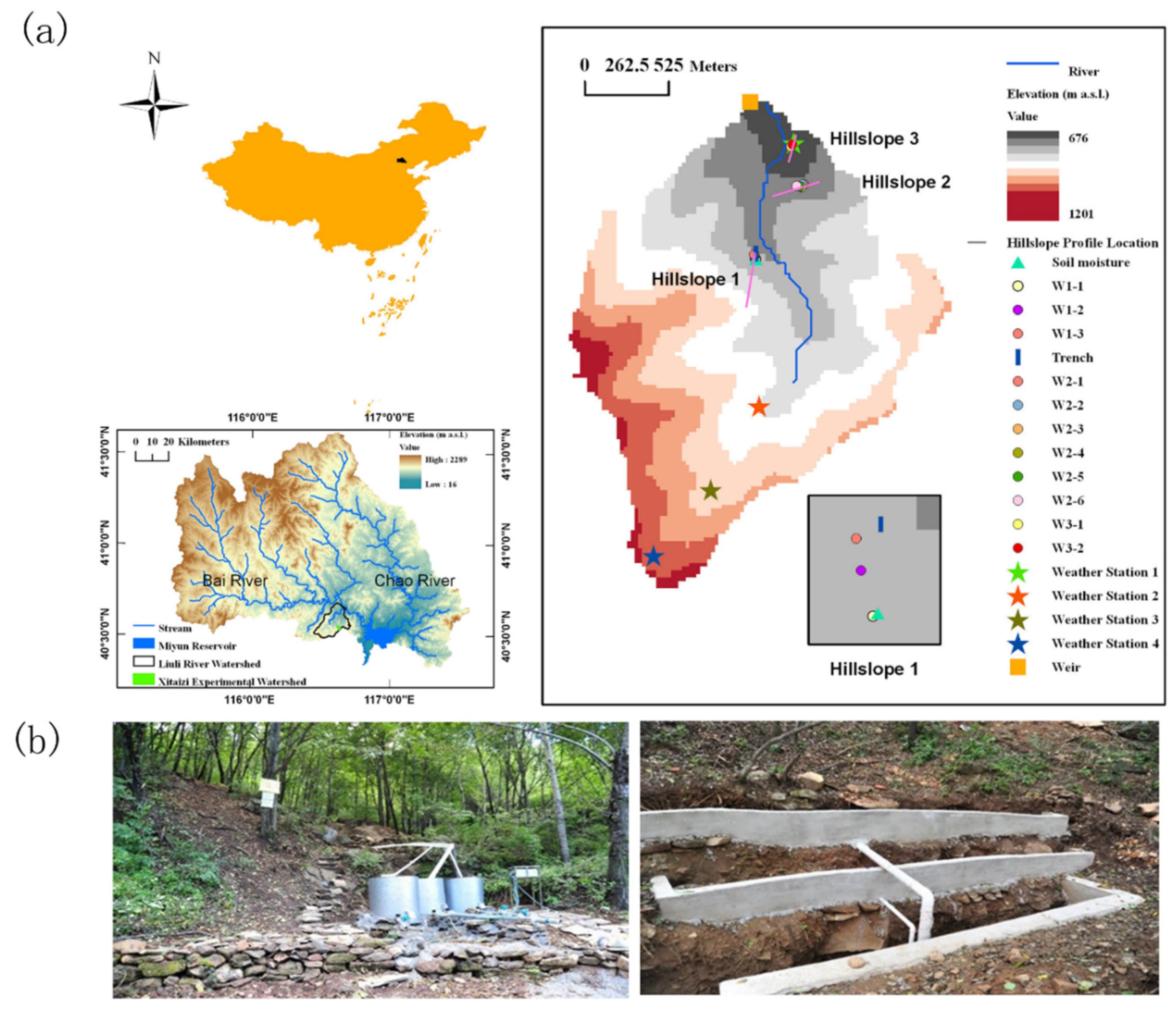
The Xitaizi Experimental Watershed (XEW) is a 4.22 km² forested catchment consisting of steep hillslopes draining to a first-order stream (Figure 1). More than half (54%) of the area has a slope of 20–40%. The catchment is almost entirely forested (98%), of which 54% is broad leaved, 2% is coniferous, 11% is mixed, the other 33% is shrubs [24].

The catchment is located at 40°32′ N and 116°37′ E, with elevation ranging from 676 to 1201 m above sea level. The regional climate of XEW is monsoon-influenced semi-humid with a humid summer and a dry winter [24]. Multi-year mean annual precipitation, air temperature, relative humidity in XEW average 625.4 mm/yr, 11.5 °C, and 59.1%. About 90% of the rainfall occurs during the warmer period from May to September, while the cooler period from October to April is relatively dry.

XEW is a typical catchment of the granitoid areas of North China: a firmly compacted, deeply but moderately weathered granite underlies approximately 80% of the catchment area. The top soil is well-drained and ranges in depth from ~0 to 1.5 m, and is mainly classified as brown earth and cinnamon soil according to Chinese soil taxonomy (these would be considered Ultisols and Alfisols under USDA soil taxonomy [25].

2.2. Meteorological and Hydrological Measurements

Meteorological data was available from 4 GRWS100 automatic weather stations (Campbell Scientific, Inc., Logan, UT, USA) spaced throughout the catchment at elevations of 700 m, 900 m, 1000 m and 1100 m a.s.l. in XEW (shown in Figure 1a). Each automatic weather station measured air temperature (T, °C), relative humidity (RH, %), wind direction and velocity at 2 m above ground surface ($u_2$, m s⁻¹), photosynthetically active radiation (PAR, $\mathsf{\mu }$mol m⁻² s⁻¹) at 10 s interval starting in 2013. Rainfall was measured at 10 min intervals by a TE525 tipping bucket rain gauge (Texas Electronics, Inc., Dallas, TX, USA) positioned close to the weather station (

Table 1. Summary of rainfall and storm runoff characteristics of 6 storm events during summer of 2014 and 2015. API represents Antecedent Precipitation Index, API (n) is the sum of antecedent precipitation index over n days, calculated as: $API\left(n\right)={{\displaystyle \sum }}_{i=1}^n\frac{P_i}{i}$, where i is the day count and P_i is the daily precipitation previously.

Characteristics	Event 1	Event 2	Event 3	Event 4	Event 5	Event 6
Event Start	29 July 2014	1 September 2014	17 July 2015	19 July 2015	31 August 2015	4 September 2015
Total Precipitation P(mm)	62	43.9	26.2	25.4	33.4	94
Rainfall Duration (hr)	6	23	7	11	25	34
Mean Intensity (mm/hr)	10.33	1.91	1.55	2.31	1.34	2.76
Peak Intensity (mm/hr)	45.6	44.85	19.8	51.24	42	39.6
Peak discharge (L/s)	31.04	28.2	8.89	11.89	15.2	20
API7 (mm)	0.1	9.1	26	42.4	4	9.9
API30 (mm)	2.6	11.5	28.4	44.8	7.6	12.4

).

Streamflow was measured using Parshall flume installed at the catchment outlet (Figure 1). Data from April 2014 to November 2015 was used in this study. Water level in the flume was measured every 10 min with a HOBO capacitance water level logger (Onset, Bourne, Massachusetts, USA). Discharge was calculated using the standard Parshall flume rating curve. Streamflow data from 18 June to 12 July 2014 was missing because of instrument failure. Data from December to March was discarded, as freezing often occurs around the gauge at that time.

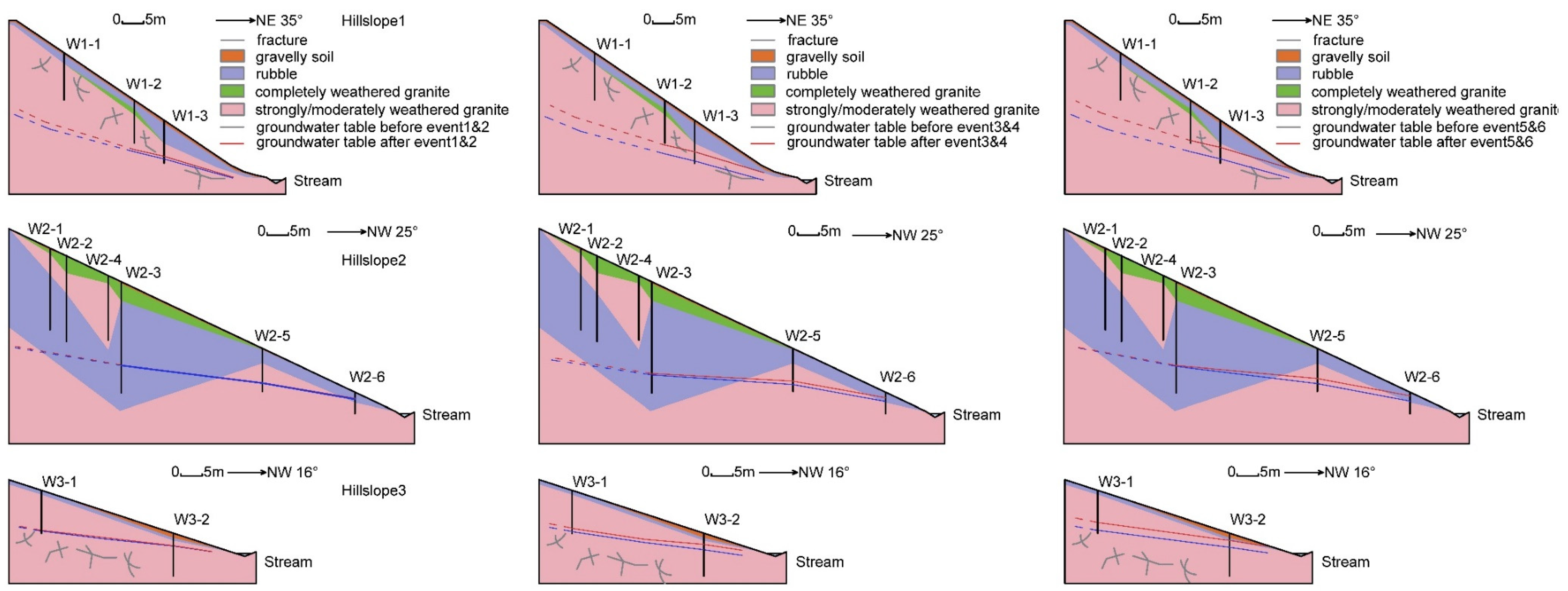
Groundwater level was measured in a network of 11 wells located on 3 hillslopes in the catchment (Figure 1 and Figure 2). The wells consisted of 8 cm diameter steel casings installed at depths between 10 m and 26 m in granite (weathered and fractured to varying extents) mantled by thin soils. The wells were screened over their entire length. Groundwater tables below ground surface ranged between 1.2 and 9.4 m, while groundwater depth near riparian area was much shallower. Slug tests conducted following installation suggested the saturated conductivity in the weathered and fractured granite was relatively high, ranging from 5.2 × 10⁻³ m/day to as high as 1.16 m/day. Water levels in the wells were recorded every 0.5–1 h using HOBO capacitance water level logger (Onset, USA). Notably, a water table was never observed in wells W1-1, W1-2, W2-1, W2-2, and W2-4 (Figure 3).

A hillslope (Hillslope 1) in the middle part of the catchment was intensively instrumented (Figure 1 and Figure 2). An 8 m long trench at the foot of Hillslope 1 (Figure 1b) was excavated to bedrock and terraced at three different depths (20, 50, 80 cm). Concrete gutters were installed on each terrace, and subsurface flow was collected through the PVC tubes draining each gutter into three tanks. The terraces were not sheltered from rainfall, and likely collected rainfall in addition to any lateral subsurface flow.

Within Hillslope 1, soil volumetric water content (VWC, %) was continuously monitored in five vertical profiles using eight CS616 time-domain reflectometry (TDR) probes installed horizontally (Campbell Scientific, Inc., Logan, UT, USA). At each profile, the probes were installed every 10 cm, down to a maximum depth of 80 cm. The 10 min mean reading has been recorded by a CR1000 data logger (Campbell Scientific, Inc., Logan, UT, USA) since 2013 (Figure 4).

2.3. Isotope Water Sampling

Samples were collected for isotope analysis (δ¹⁸O and δ²H) in six summer storm events. Two storms (Events 1 and 2) were sampled in July and September 2014 and four (Events 3–6) in July–September 2015. We considered rainfall events separated by at least 15 h and determined a streamflow response.

Stream water and rainfall samples were collected every 1 h during rainfall storms using two automated samplers (ISCO6712, Inc., Lincoln, Nebraska, USA) installed at the outlet of the catchment near the weir. Stream water sampling was initiated a few hours prior to each storm event.

Subsurface flow samples from Hillslope 1 were collected manually from the three trench tanks every ~6 h during each storm. In Events 3–6, an automated sampler was used to collect samples from the 50 cm terrace every hour. Flow volume in the trench was not recorded.

Groundwater and soil water were sampled as bulk samples manually at different intervals ranging from 3–9 h. Soil water was collected from suction lysimeters installed in three vertical profiles on Hillslope 1 at six depths (10, 20, 30, 40, 50, 80 cm). Soil water samples were collected by applying a suction of −17 kPa. At many sampling times only a few suction lysimeters yielded soil water after several hours of suction. Typically, no soil water could be collected in the hours prior to each rainfall event, and no soil water could be collected at 40–80 cm depth after small rainfall events.

In addition to sampling on event scale, rainwater, groundwater and stream water sampling were conducted biweekly during the wet season (May to September) and monthly during the dry season (October to April) in 2014–2015. Groundwater (from wells) and stream water bulk samples were collected manually. Bulk rainfall was collected with a 10 cm diameter polypropylene funnel and draining to a 4 L high density polyethylene bottle. A ping pong ball was placed in the mouth of funnel to reduce evaporation [26].

2.4. Laboratory Analysis

The δ¹⁸O and δ²H values of collected samples were analyzed by the Hydrology Laboratory in Tsinghua University [27] using a Picarro L2130i wavelength-scanned cavity ring-down spectroscopy (WS-CRDS) analyzer. The measurement precision of the instrument is ±0.1‰ and ±1‰ for δ¹⁸O and δ²H, respectively. The isotope values of water are reported as per mil (‰) units relative to the Vienna Standard Mean Ocean Water (VSMOW) [28]. To ensure the accuracy of isotope analysis, each vial was analyzed 6 times. The first three results were discarded to avoid memory effects [29]. One standard vial (VSMOW) was analyzed for every four samples. Results from analysis of standards at the start and end of each run were compared to check for drift in the analyzer.

2.5. Hydrograph Separation

The two-component hydrograph separation method [30,31] was applied to partition storm runoff into pre-event/old water and event/new water via the following mixing equations:

$$Q_t=Q_p+Q_e$$

(1)

$$Q_t{C}_t=C_p{Q}_p+C_e{Q}_e$$

(2)

$$Q_e=Q_t\ast \frac{C_p-C_t}{C_p-C_e}$$

(3)

where Q_t, Q_e and Q_p are the assumed components of total storm water runoff (runoff at time t, event water and pre-event water), and C_t, C_e, and C_p are the corresponding δ¹⁸O/δ²H isotope concentrations.

The use of a two-component model for hydrograph separation requires the following assumptions to be true [3,32,33]: (1) δ¹⁸O or δ²H values are significantly different in pre-event and event water, (2) tracer concentrations of pre-event and event water are constant in space and time (or the variations can be accounted for), (3) additional component contributions (e.g., soil water) are negligible, or the isotopic signature of the soil water must be similar to that of groundwater. (4) the tracers mix conservatively, and (5) surface storage contributes minimally to the streamflow. We assumed the pre-event water isotope composition C_p was characterized by the base flow samples collected 2–3 h prior to the storm. The rainfall or new water tracer component C_e was calculated using the incremental mean weighting method [34]. These concentrations were distinct in each event. Baseflow concentrations typically returned to the same value as prior to the storm, suggesting they were constant, and the incremental mean method provides some adjustment for the changing rainfall concentrations. The assumption that contributions from soil water were negligible was supported by soil moisture data, which showed that the deepest soil layers either did not respond to rainfall events, or they responded well after the rainfall event had ended and storm discharge subsided. Water isotopic tracers mix conservatively, and fractionation effects on catchment discharge are commonly believed to be small [2].

The uncertainty of event water/pre-event water contribution fractions in streamflow was calculated through a general uncertainty propagation technique [35].

$${\sigma }_{fe}=\sqrt{{\left[\frac{f_p}{\left(C_e-C_p\right)}{\sigma }_{cp}\right]}^2+{\left[\frac{f_e}{\left(C_e-C_p\right)}{\sigma }_{ce}\right]}^2+{\left[\frac{-1}{\left(C_e-C_p\right)}{\sigma }_{ct}\right]}^2}$$

(4)

where $\sigma$ is the uncertainty, f_e/f_p is the event/pre-event water fraction in storm runoff, C refers to the isotopic signature and subscripts e, p, and t refer to event (new) water, pre-event (old) water and stream water (total), respectively.

Assuming that sample collection did not introduce any measurement uncertainty, ${\sigma }_{ct}$ was set at the laboratory precision of the isotope analyses: 0.1‰ for δ¹⁸O and 1‰ for δ²H [35]. The uncertainty of event water ${\sigma }_{ce}$ and pre-event water ${\sigma }_{cp}$ for ¹⁸O and δ²H were each set to the standard deviation of the observations (

Table 2. Maximum (Max), minimum (Min), mean ± standard deviation (Mean ± SD) values of isotopic compositions (δ¹⁸O and δ²H, ‰) of rainfall water, stream water, base flow, soil water and groundwater corresponding to 6 storm events. Here n refers to total number of samples, soil water isotope ratios at all depths were included. Base flow is defined as all samples collected 2 h prior to the start of rainfall [18].

	δ18O (‰)	Event 1					Event 2					Event 3
δ2H		Mean	Min	Max	SD	n	Mean	Min	Max	SD	n	Mean	Min	Max	SD	n
rainfall		−8.36	-	-	-	1	−8.82	-	-	-	1	−12.36	−15.96	−9.29	2.34	6
river		−9.71	−9.88	−8.86	0.20	53	−9.73	−9.97	−8.67	0.23	77	−10.32	−11.65	−9.63	0.44	18
soil		−7.84	−8.16	−7.19	0.26	12	−7.09	−7.54	−6.03	0.40	13	−7.07	−7.57	−6.65	0.36	5
groundwater		−9.67	−9.70	−9.63	0.03	4	−9.65	−9.66	−9.64	0.01	5	−10.11	−10.14	−10.07	0.04	2
baseflow		−9.82	−9.88	−9.79	0.03	7	−9.94	−9.95	−9.94	0.01	2	−10.19	-	-	-	1
throughflow		-	-	-	-	-	-	-	-	-	-	−11.89	−15.15	−8.69	2.69	10
rainfall		−53.62	-	-	-	1	−57.96	-	-	-	1	−85.09	−119.5	−56.21	16.11	6
river		−65.20	−66.40	−58.73	1.54	53	−65.61	−68.60	−56.16	1.81	77	−69.55	−81.24	−65.32	3.88	18
soil		−54.19	−56.87	−50.53	1.87	12	−46.86	−51.10	−41.66	2.86	13	−47.37	−49.69	−43.73	2.23	5
groundwater		−64.81	−64.93	−64.60	0.13	4	−64.70	−65.00	−64.29	0.27	5	−67.56	−67.79	−67.33	0.23	2
baseflow		−66.05	−66.40	−65.88	0.15	7	−68.01	−68.60	−67.42	0.59	2	−67.83	-	-	-	1
throughflow		-	-	-	-	-	-	-	-	-	-	−85.06	−112.8	−57.97	22.64	10
	δ18O (‰)	Event 4					Event 5					Event 6
δ2H		Mean	Min	Max	SD	n	Mean	Min	Max	SD	n	Mean	Min	Max	SD	n
rainfall		−11.56	−12.27	−10.93	0.52	7	−13.3	−14.7	−10.1	1.53	14	−14.1	−17.6	−9.6	2.51	25
river		−10.24	−10.61	−10.12	0.13	26	−10.1	−10.5	−9.9	0.15	30	−10.8	−12.1	−10.1	0.57	43
soil		−8.29	−9.56	−7.13	0.70	24	−8.3	−8.6	−8.0	0.28	4	−10.5	−13.9	−8.3	1.66	40
groundwater		−10.17	-	-	-	2	−9.9	−9.9	−9.9	0.02	3	−9.8	−9.8	−9.8	0.02	4
baseflow		−10.12	−10.12	−10.11	0.01	1	−10.0	-	-	-	1	-	-	-	-	-
throughflow		−11.43	−12.46	−10.39	0.58	12	−13.0	−14.3	−11.9	0.90	8	−14.0	−17.0	−10.2	1.90	29
rainfall		−81.45	−89.45	−74.80	6.03	7	−93.6	−106.3	−64.7	14.03	14	−100.6	−129.2	−68.4	19.18	25
river		−68.56	−71.97	−67.64	1.24	26	−67.7	−70.7	−65.6	1.29	30	−73.6	−84.7	−67.7	4.64	43
soil		−56.07	−66.44	−49.09	4.74	24	−56.4	−57.3	−55.6	0.81	4	−71.5	−98.8	−11.0	15.71	40
groundwater		−67.60	−67.62	−67.59	0.01	2	−65.4	−65.9	−64.8	0.47	3	−65.0	−65.0	−64.9	0.05	4
baseflow		−67.85	-	-	-	1	−66.8	-	-	-	1	-	-	-	-	-
throughflow		−79.89	−89.05	−71.71	5.58	12	−92.1	−102.5	−83.4	7.41	8	−98.9	−123.0	−72.4	14.49	29

). Uncertainty analysis results for all storm events are listed in

Table 3. Pre-event water contributions to storm runoff using one-tracer, two end-member hydrograph separation (δ¹⁸O and δ²H, ‰), and corresponding uncertainty analysis. σ is the uncertainty, f_e/f_p is the total event/pre-event water volume over total storm runoff volume, f_e-max is the maximum event water fraction, C refers to the isotopic signature and subscripts e, p, and t refer to event water, pre-event water and stream water, respectively.

Summary	Event 1		Event 2		Event 3		Event 4		Event 5		Event 6
	δ18O	δ2H	δ18O	δ2H	δ18O	δ2H	δ18O	δ2H	δ18O	δ2H	δ18O	δ2H
Ce (‰)	−8.36	−53.6	−8.82	−58	−12.11	−81.4	−12.38	−86.70	−11.01	−72.11	−12.5	−89.59
Cp (‰)	−9.82	−66.1	−9.94	−68	−10.19	−67.83	−10.17	−67.85	−9.98	−66.79	−9.84	−65.03
fp	0.63	0.67	0.84	0.81	0.770	0.678	0.955	0.940	0.81	0.75	0.65	0.66
fe	0.37	0.33	0.16	0.19	0.230	0.322	0.045	0.060	0.19	0.25	0.35	0.34
fe-max	0.66	0.59	0.99	0.99	0.76	0.99	0.2	0.24	0.54	0.7	0.87	0.8
σfe	0.07	0.08	0.09	0.11	0.29	0.39	0.05	0.06	0.29	0.38	0.33	0.27
runoff new water volume(m3)	189.9	167.23	233.77	260.77	42.73	59.95	18.12	23.83	107.77	149.6	690.73	673.69
Contributing Area (m2)	3064	2697	5325	5940	1631	2288	714	938	3227	4479	7348	7167
Contr. area per channel length (m²/m)	1.46	1.28	2.54	2.83	0.78	1.09	0.34	0.45	1.54	2.13	3.50	3.41

.

The effective fraction of the catchment contributing event water was obtained by integrating the area under the event water curve and dividing this by the total rainfall volume. This was converted to an effective area by multiplying this fraction by the catchment area (4.2 km²). The (approximate) effective contributing area per channel length was then determined by dividing the effective area by the length of channel in the watershed (~2.1 km).

3. Results

3.1. Hydrological Dynamics during the Study Period

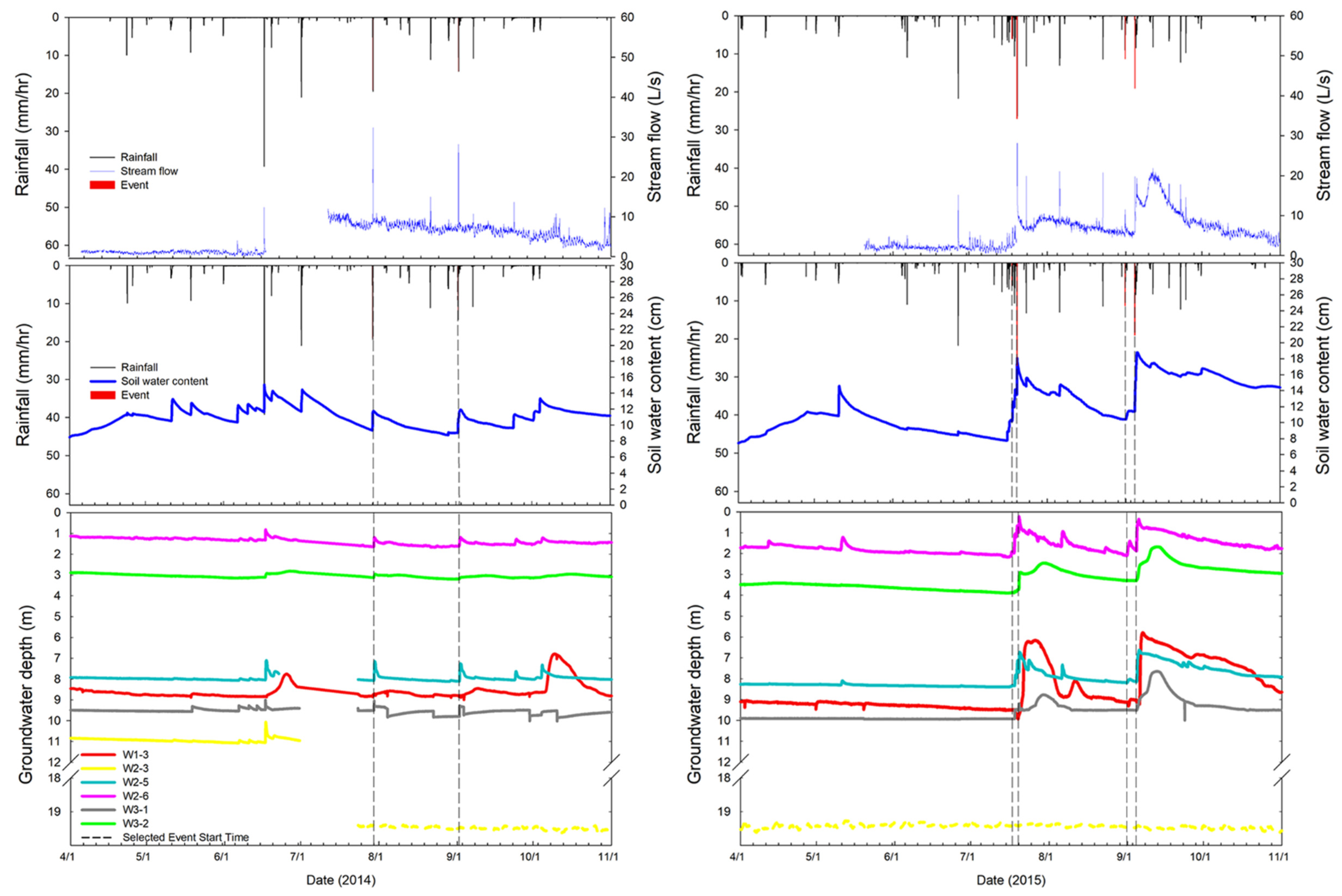
In 2014 and 2015, total rainfall (P) was 451 mm/yr and 650 mm/yr, of which about 89% and 91% fell during the wet season (May–September). The rainfall time series and hydrograph from 1 April 2014 to 1 November 2015 is shown in Figure 3. Discharge is low at the start of each wet season (1–4 L/s) and did not respond substantially to small and moderate-sized rainfall events during it. These events generated only brief increases in discharge that subsided almost immediately after rainfall ceased.

The discharge increased after three very large rainfall inputs. A 41.1 mm event on 17 June 2014 appears to have increased discharge, though data is not available until 12 July when the discharge is 12 L/s. The discharge continues to recede almost monotonically over the next 5 months. In 2015 two events appear to have increased discharge. A total of 147 mm falling over 17–23 July led to a rapid rise in discharge, followed by a fall and a subsequent second rise that peaks 9 days after the first. A storm of 128 mm over 4–6 September also produced a rise in discharge, followed by a fall and a second peak on 10 September, 5 days later. The second discharge peak on 10 September is not associated with any recorded rainfall, and only 11 mm falls in the 5 days prior to it.

Only the wells at or near the toe of each hillslope transect responded to rainfall events (W1-3 in Hillslope 1, W2-5 and W2-6 in Hillslope 2 and W3-2 in Hillslope 3). Well 3-1 was highly transient, and water table was only observed in heavy storms. Well 2-3 had a water table at a depth of 19.3 m after July 2014, and did not respond to rainfall inputs. Wells further upslope remained dry during the whole study period.

The downslope observation wells of the three hillslopes showed that the water table responded differently in 2014 than in the slightly wetter 2015 (Figure 3). In 2014, the water tables did not respond to events prior to the large storm on 17 June 2014 that also seems to have triggered the rise in discharge for that year. In that event and in four later large events, the water table in Hillslope 2 (wells W2-5 and W2-6) increased sharply (0.3–1 m) around 6 h after the rainfall event. Subsequently the water table receded rapidly at first, then slower. The response in Hillslope 1 (well W1-3) was more muted, rising and falling slowly over several days after large events. In Hillslope 3 (well W3-2), there was both a small rapid initial response, and a secondary rise some days later.

The groundwater tables at the start of the wet season of 2015 were initially lower than they were in the corresponding period of 2014 of about 0.5–1 m. The first and largest rise in groundwater occurred on 20 July, again triggered by the large storm that initiated the streamflow response for the year (Figure 3). Water tables in all downslope wells increased by 0.8–1 m within 3 h. The water tables declined gradually, responding transiently to a small storm in early August before rising and remaining high in response to the 4 September storm. Hillslope 2 showed the most rapid response to rainfall, but unlike the previous year the rise following the two large events persisted, receding slowly over several weeks. Hillslope 1 again showed a more delayed response to the first event, but the response to the 6 September event was more rapid, and the recession was slower than previous large events. The response in Hillslope 3 was also larger than in the previous year, but the form of the response was largely similar, with a sharp initial rise followed by a secondary peak, and then a slow recession. The secondary peak in Hillslope 3 seemed to coincide with the secondary peak in streamflow observed at the nearby catchment outlet.

3.2. Hydrologic Dynamics of Intensively Sampled Events

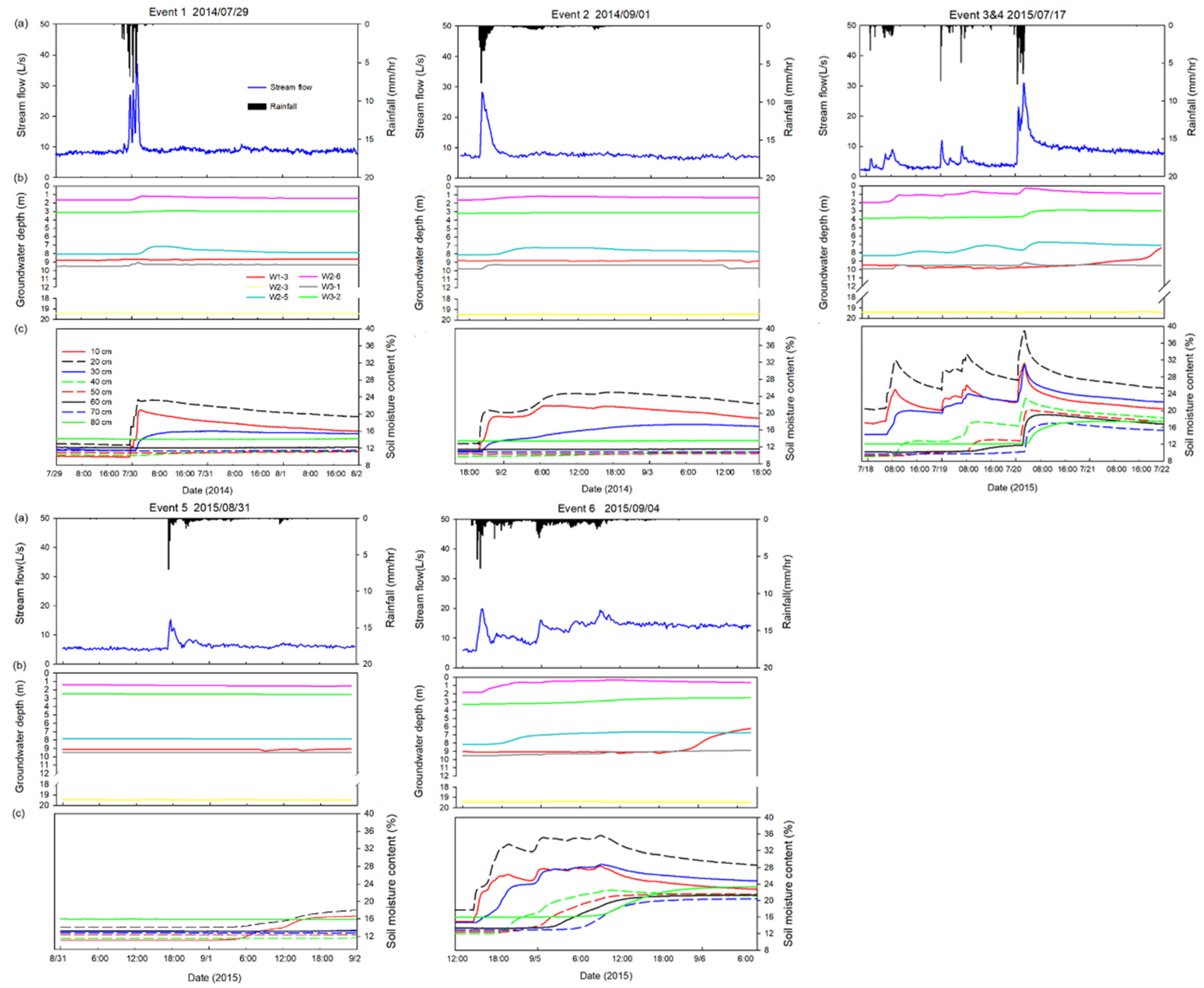
Characteristics of the six intensively sampled storm events are summarized in Table 1. Events 1 and 2, occurring in 2014, and were moderate storms with dry antecedent conditions that produced small groundwater responses in all three hillslopes, but did not substantially change the discharge. Events 3 and 4 were smaller storms that occurred in rapid succession in July 2015, but antecedent rainfall was higher for these two events than for the first two, and they were followed by a large and sustained increase in discharge. Event 5 was slightly larger than the previous two, but fell on a drier catchment, and produced a relatively small groundwater and streamflow response. Six days later, Event 6 dropped a large amount of rainfall on the catchment (94 mm) and produced the largest rise in discharge and in Hillslope water tables. Peak and mean 10-min rainfall intensity ranged from 39–52 mm/hr and 1.55 to 10.3 mm/hr.

The soil moisture (volumetric water content %, VWC) in Hillslope 1 showed an increase of 10 to 20% in shallow depths (10 to 30 cm) in all six storms, but no response to rainfall in deeper soil layers (60 to 80 cm) in Events 1, 2 and 5 (which all have low antecedent rainfall) (Figure 4). Lag time between rainfall peak and soil water responses became longer with deeper soil layers. In Events 1 and 2, soil moisture at 10–20 cm increased immediately in response to rainfall and declined gradually, and soil moisture at 30 cm increased gradually, while the other depths presented no variations. In Event 5, only soil water at 10 cm and 20 cm responded to rainfall. This suggests rainwater infiltrated and was redistributed only in these shallow layers during these events. In Events 3 and 4, the hillslope was much wetter, with an antecedent precipitation index over 7 days (API7) of 26 mm. As these storms progressed, soil water in deeper layers increased and remained high after the storms ended. This suggests deeper infiltration occurred during these storms. In Event 6, the soil moisture at 10, 20 and 30 cm increased more than 50% during the storm, and varied rapidly with changes in rainfall intensity. Deep layers were slower to react but increased significantly by the end of the storm. During the recession period, soil moisture in the shallow layers decreased faster than in deep layers. In deep soil layers, water tended to remain high between events.

3.3. Isotope Dynamics of Intensively Sampled Events

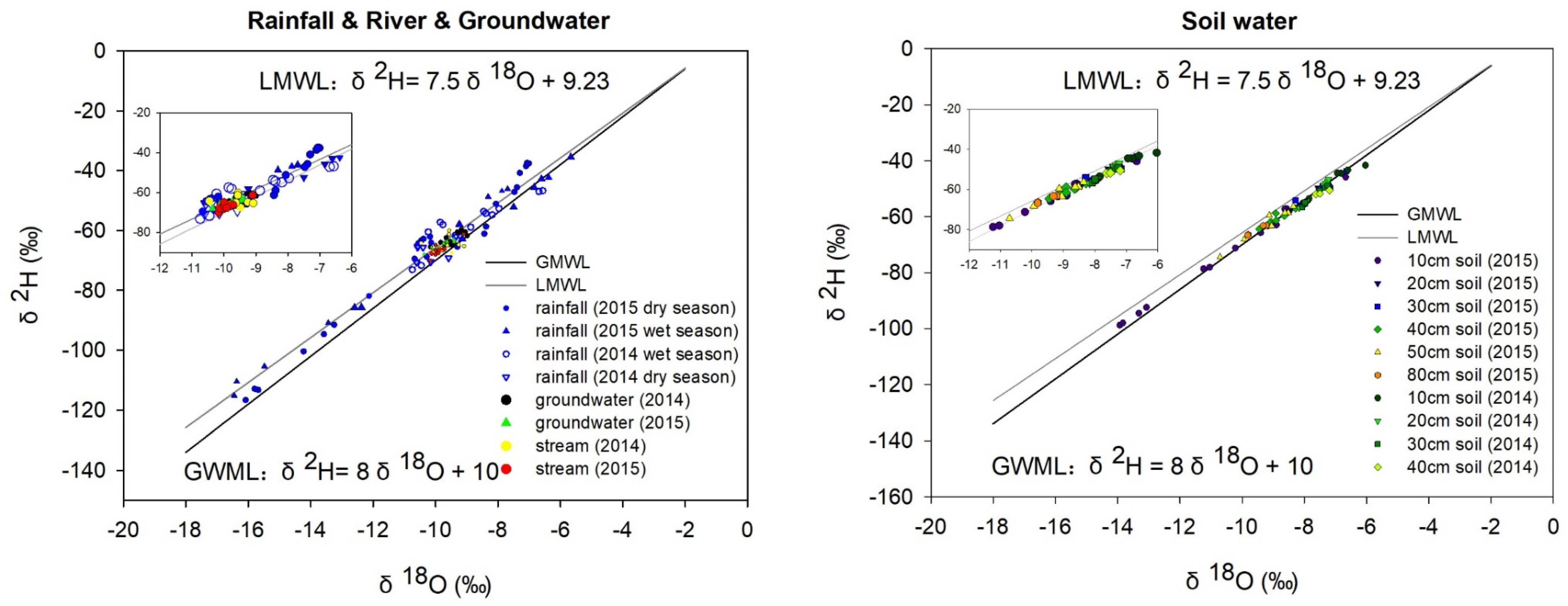
The δ¹⁸O and δ²H values of all biweekly rainfall samples, river water, groundwater and soil water samples, taken in the period from April 2014 to November 2015, are shown in Figure 5. The Local Meteoric Water Line (LMWL, δ²H = 7.5δ¹⁸O + 9.23‰, n = 63, r² = 9.67) coincides well with Global Meteoric Water Line (GMWL, δ²H = 8δ¹⁸O + 10‰) [36]. The isotope ratios of stream water were all plotted on the LMWL, while those of soil water were plotted very slightly below, suggesting a minor amount of evaporative enrichment. There is some difference between biweekly volume-weighted values of rainfall in the wet seasons of 2014 (−8.6‰ for δ¹⁸O and −58.3‰ for δ²H on average) and 2015 (−10.1‰ for δ¹⁸O and −67.3‰ for δ²H on average), probably caused by different moisture origins of precipitation [37,38]. Temporal variability of isotope ratios in rainwater was large between events during the study period but no clear seasonal trend could be detected. Extreme isotopic values occurred in large and long storms. Variability of meteoric δ¹⁸O and δ²H was larger in 2015 versus 2014 (standard deviations of 3.06‰ and 24.24‰ versus 1.32‰ and 8.62‰, respectively). The seasonal variation in rainwater isotope ratio was not discernable in the biweekly base flow samples, which were tightly constrained to a narrow range (−9‰ to −11‰ for δ¹⁸O, and −65‰ to −68‰, for δ²H). Groundwater samples from well had a similar isotopic composition to streamflow (Table 2), suggesting that streamflow is probably dominated by bedrock groundwater. Soil water isotope signatures were strongly lagged and damped in the deep soil profile, while shallow soil water interacted more with rainfall during the wet season.

During the six intensively sampled events, isotope ratio in stream flow changed rapidly (Figure 6). In Events 3–6 of 2015, isotopic compositions of rainfall water were more negative compared to the previous events, with a mean of −14.51‰ for δ¹⁸O and −32.48 ‰ for δ²H, respectively. The lowest δ¹⁸O and δ²H values in rainfall and stream flow were associated with Event 6, which also showed pronounced within-storm variability.

The δ¹⁸O and δ²H values of soil water did not show clear spatial patterns during storm events, but tended to become more negative over the course of the 2015 season (Figure 5). In all events apart from Event 6, the soil water was substantially more enriched than the rainfall or the stream water.

Throughflow at the Hillslope 1 trench (sampled only in Events 3 to 6) was nearly identical isotopically to rainfall. This suggests that either the trench is sampling rapid lateral preferential flow through the subsurface, or (perhaps more likely) it is showing the influence of rainfall falling on the (unsheltered) terraces of the trench collection system. Since the volume of throughflow was not recorded, it is difficult to say whether the volume of apparent throughflow was small enough to support either possibility. However, given that throughflow samples were obtained from nearly the very first moment it rains in each event, it seems likely that the throughflow trench was collecting some amount of rainfall.

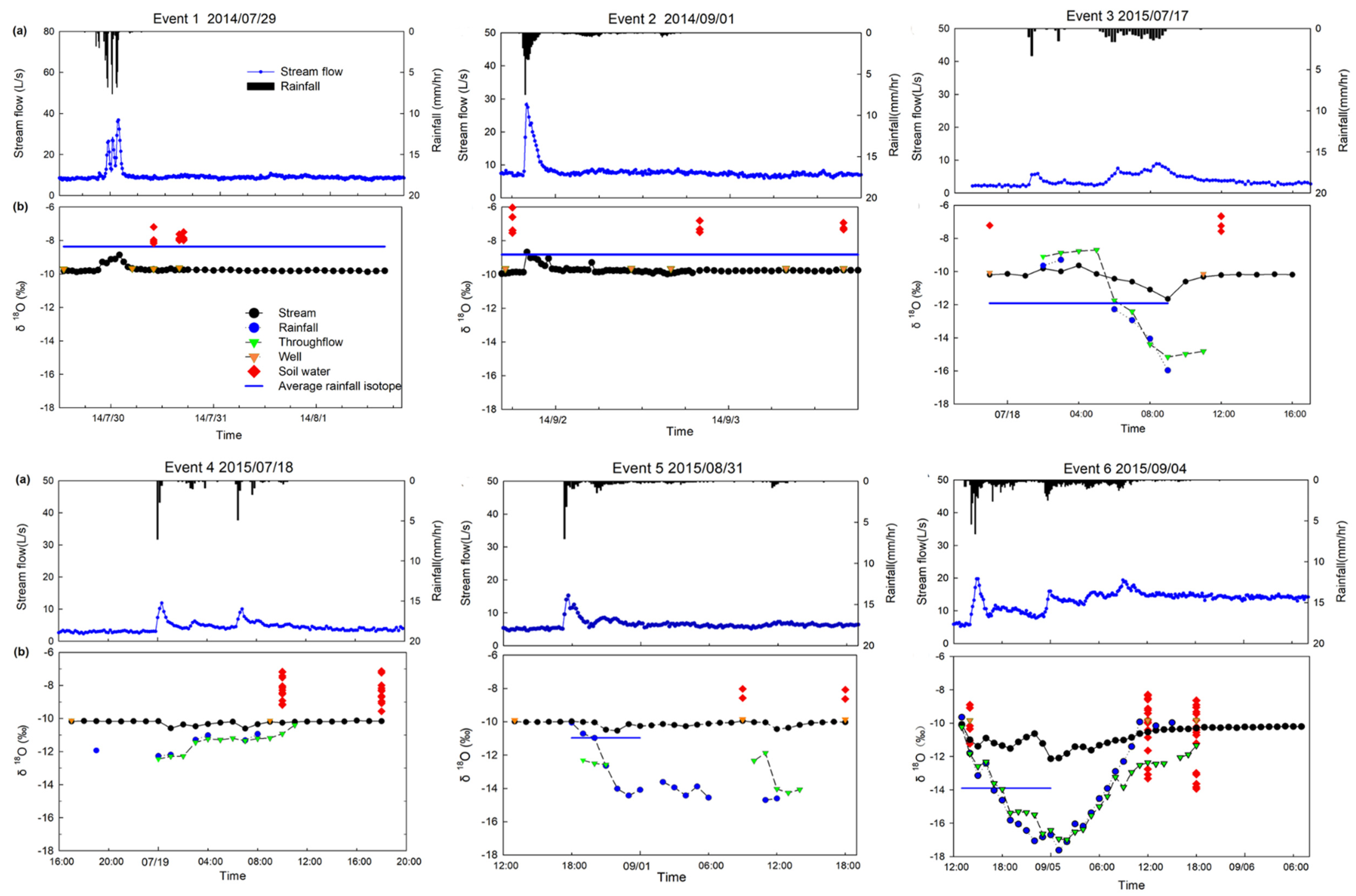
3.4. Data Presentations of Intensively Sampled Events

The hydrograph, variations in rainwater, stream water, soil water and groundwater δ¹⁸O values are presented in Figure 6. In Event 1, the discharge before rainfall began was ~8.5 L/s. Peak discharge of 36.8 L/s occurred around 30 min after peak rainfall. Rainfall δ¹⁸O (−8.36‰) was higher than that of stream water throughout the event. Stream water isotope values at peak runoff (−8.86‰) were higher than base flow (−9.81‰). The δ¹⁸O values in stream water increased as soon as the rainfall started and returned to the base flow value rapidly after the storm event ended.

Event 2 was similar to Event 1 in many respects. Base flow runoff before precipitation commenced was ~7.5 L/s. The peak discharge of 28.2 L/s was observed 20 min after the peak rainfall intensity. The incremental volume-weighted rainfall isotope value (−8.82‰) was higher than stream water at the start (−9.91‰) and 0.15‰ lower than stream flow at runoff peak (−8.67‰). Stream δ¹⁸O began at −9.94‰, and rose immediately with the discharge rising limb to a peak of −8.67‰. After the storm ended, the stream isotope decreased to the initial level as discharge decreased.

The rainfall and hydrograph for Event 3 was different, with two multiple rainfall and streamflow peaks. Streamflow before the event was ~3 L/s. The first runoff peak (5.9 L/s) occurred immediately after the first precipitation peak (3 mm/10 min) at 1:20 a.m., while a second runoff peak of 8.8 L/s was observed in response to a subsequent period of lower-intensity rain 7 h later. Stream flow returned to the baseflow condition more gradually than in the previous two events. The isotopic compositions of rainfall in Event 3 showed large temporal variations. As the storm event went on, the heavy isotopes in rainfall water became depleted (perhaps due to Rayleigh fractionation [36]). The δ¹⁸O values of rainfall fluctuated near −9.4‰ at the start of the event (slightly more enriched than the stream water) and decreased all the way to −15.9‰ by the end of the storm. In response to rainfall, the stream water isotopic composition at the beginning fluctuated first upward during the first peak of discharge, and then down to a low value at the second runoff peak of −11.6‰.

In Event 4, runoff again responded quickly to rainfall and presented similar variation trend with rainfall pattern. Base flow discharge was ~3 L/s following Event 3. The first runoff peak of 11.9 L/s was observed 20 min after the first rainfall peak (occurred at 0:00 a.m., 18 July,). A second rainfall peak occurred 6.5 h after the first rainfall peak, with an intensity of 4.9 mm/10 min. Lag time between second runoff peak and second rainfall peak was also 20 min. Fluctuations of δ¹⁸O in rainfall was relatively small compared to Event 3, with values ranging between −12.66‰ and −10.93‰. Stream isotope showed some small temporal variations toward the rainfall signal during peak discharge. The δ¹⁸O values of stream water at two runoff peaks were 0.5‰ lower than that of base flow (−10‰).

In Event 5, base flow discharge was higher than in the previous two events, at ~5.3 L/s. A single runoff peak of 15.2 L/s was observed in response to the rainfall peak. The lag time between runoff and rainfall peaks was 20 min. The rainwater δ¹⁸O value was lower than that of stream water throughout the event. Unlike in previous events, the stream water δ¹⁸O value at peak runoff (−9.98‰) was very similar to that of base flow and initial rainfall water, and had not appeared to respond to the more isotopically depleted rainfall. However, some 4 h later, in response to a period of less intense rainfall, the stream isotope value (−10.5‰) did drop toward the rainfall. This occurred again 14 h later. The δ¹⁸O values in stream water increased back to the initial base flow value quickly after these fluctuations.

Event 6 was a larger and more protracted rainfall event. Base flow runoff before precipitation commenced was ~5 L/s, but (unlike other events) did not return to this value after the event, instead remaining high at around 14 L/s. The first peak runoff of 17.1 L/s was observed 10 min after rainfall peak. The rainfall intensity declined after that first peak to a relatively steady rate for around 12 h, but the runoff amount gradually increased (with several peaks). The δ¹⁸O in rainfall began high (−9.64‰), decreased to a low in the middle of the event (−17.05‰), and then increased again (−9.96‰). Stream water isotope values fluctuated between −10 and −12.1‰, with the lowest value of −12.1‰ observed 9 h after the peak runoff, coincident with the lowest values in rainfall.

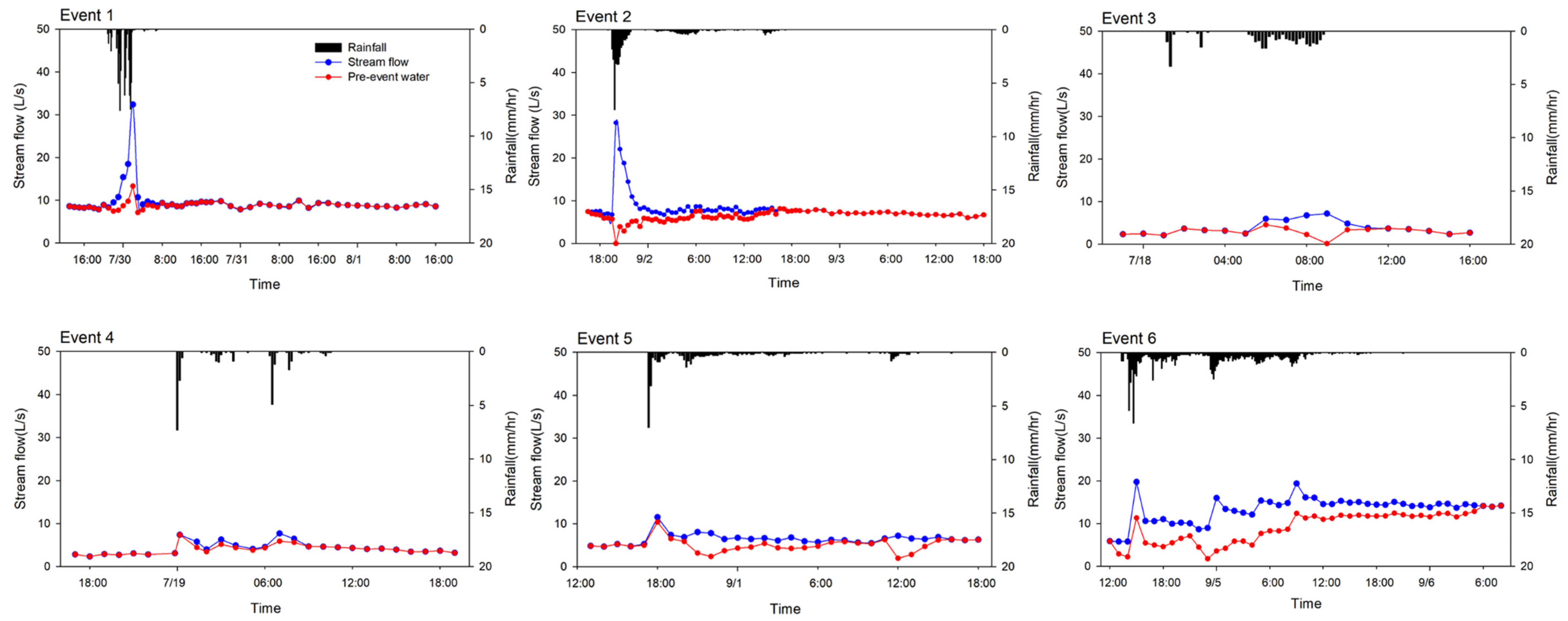
3.5. Two-Component Hydrograph Separation and Effective Contributing Area

In general, differences between the pre-event water proportions derived by δ²H and δ¹⁸O were small (1–6%, shown in Table 3, Figure 7). Event water fractions (f_e) varied between 5% and 37% in 6 events. The smallest event-water contribution (5%) occurred in Event 4. It is noticeable that Event 3 and Event 4 happened on two subsequent days and shared similar duration, total rainfall, and rainfall intensity patterns, but Event 4 was almost entirely dominated by pre-event water. The largest event-water fractions appeared in Event 1 and Event 6. Uncertainty in event and pre-event water fractions were estimated from Equation (4). Event water fraction uncertainty was larger for large-amount and long-term storms with large fluctuations in isotopic composition over the duration of the storm, so that uncertainty in f_e for Event 1 is ±7%, while for Event 6 it is ±30%. The effective contributing area of the storms varied from around 800 m² (or 0.02% of the total area) for Event 4 up to 7200 m² (or 0.17% of the total area) for Event 6.

4. Discussion

Based on the results presented above, we can start to piece together a picture of how the water that will ultimately become discharge moves through this watershed.

At first glance, it is not clear why the six intensively sampled events have such different event and pre-event water compositions. Event 3 and Event 4 happened very close together in time, and shared similar duration, total rainfall, and within-storm rainfall intensity patterns, but Event 4 was almost entirely pre-event water dominated. In contrast, Event 1 and Event 6 had very similar (large) event water fractions, but were very different storms. The first was intense and brief (62 mm in 6 h) and fell on an extremely dry catchment, while the last was long (94 mm in 34 h) and fell on a catchment that was already moderately wet.

These odd patterns in fraction of event water become more explicable if we instead consider how event water discharge might be generated in the catchment. Storm runoff from humid, forested, upland catchments is generally conceptualized as arising from two source areas: riparian zones and hillslopes [17]. The data from XEW seem to suggest that hillslopes contribute negligible volumes of water to event hydrograph of these storms, either as event water or as mobilized pre-event water. The effective contributing area of event water based on the isotope hydrograph separation is a very small fraction of the catchment, and represents only 0.34–3.5 m per meter of channel length in the catchment. Furthermore, even though this event water does not make up the majority of discharge during the storm period, it represents almost all the area under the hydrograph peak and above the baseflow discharge. The exception to this is Event 6, in which the baseflow discharge changes considerably over the course of the storm. The contribution of pre-event water began a sustained rise around 18 h after the storm began, eventually reaching the post-event baseflow discharge, in which the contributions of recent event water are not distinguishable. This could be because the dynamics of the non-saturated layers were different between events [39,40].

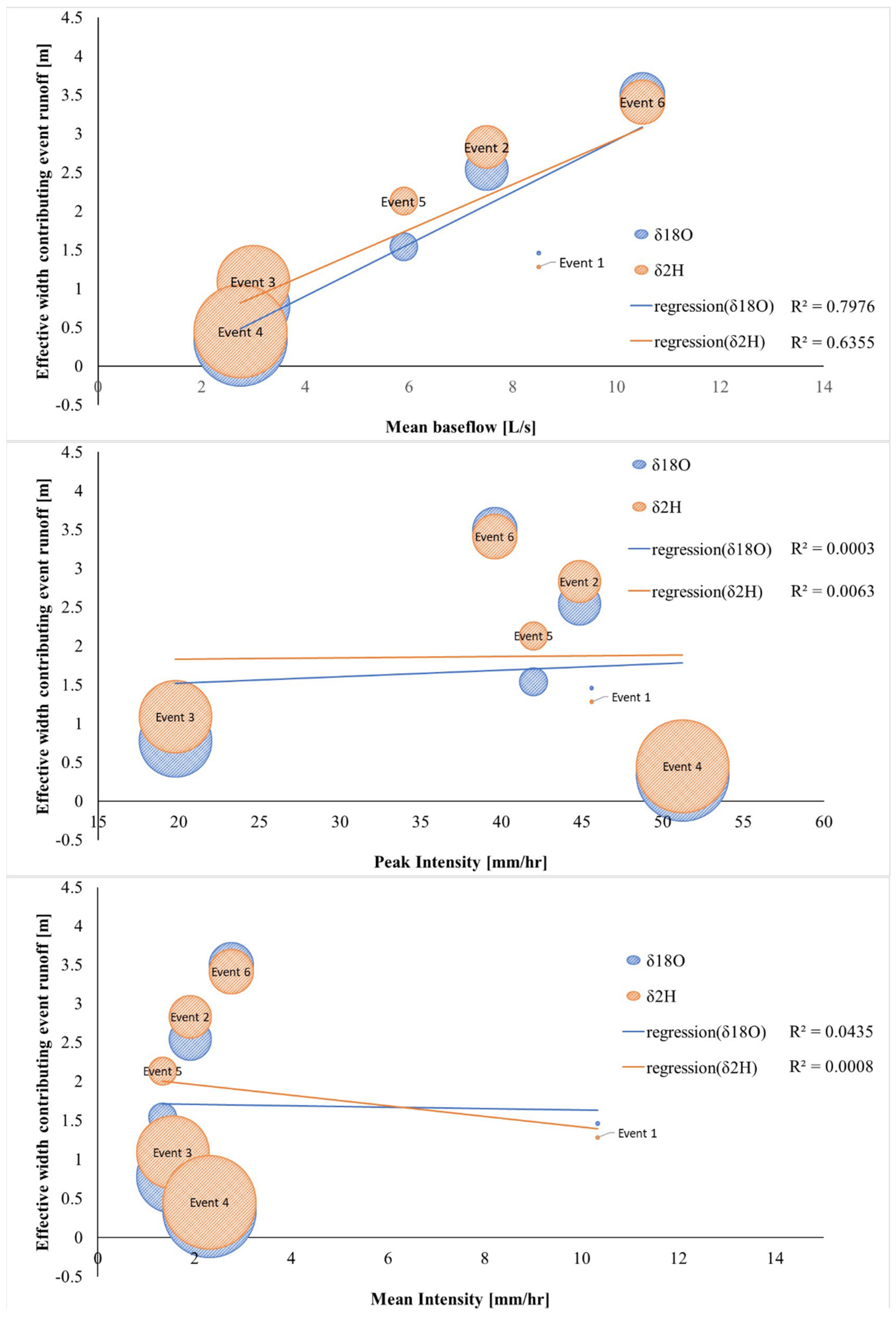
Given that this is a catchment in a relatively dry climate (at least for part of the year), we should consider the possibility that the mechanism generating runoff in the small areas contributing event water is Hortonian infiltration excess. If this were the case, we would expect to see some relationship between rainfall intensity (either mean or maximum) and the fraction of rainfall that departs as contributing area per channel length. Figure 8 shows these relationships, with the size of each bubble also indicating the antecedent wetness (API7) for reference. There is no relationship with mean intensity and peak intensity.

On the other hand, the event-water runoff ratio does show a very tight positive relationship with the mean baseflow (Figure 8). Mean baseflow here is the average of the streamflow before and after the event water passes through the system, and is nearly identical to the pre-event discharge in all but Event 6. This strong relationship suggests that the catchment processes that determine the baseflow rate also determine the fraction of rain that leaves immediately as stream discharge. This is likely areas of surface (or very-near-surface) saturation where baseflow is seeping out of the ground. Event 1 is an outlier in the relationship, falling well below the line that the other events appear to follow. However, this event had an extremely dry antecedent wetness, suggesting that Event 1 water was sequestered in some unrequited storage that was filled with later events.

Low event water fraction and baseflow dominating storm runoff is not typical of catchments with such low rainfall. Runoff in relatively arid areas is typically dominated by Horton overland flow due to the low density of vegetation [41,42]. Here the forest allows for high infiltration rates, and the deeply weathered rock allows for substantial subsurface storage. These two facts may be related—several studies have pointed to the importance of ‘rock moisture’ for sustaining vegetation in seasonally dry climates [43].

It is possible that our estimates of event water contributions are incorrect due to a failure to account for an additional source—soil water mobilized into the stream, in particular. Soil water had a lighter isotopic composition than either streamflow or precipitation in all but Event 6, when it was indistinguishable from streamflow. Contributions from a soil water end member would mean that compared to our current estimates, the true event water contributions would need to be smaller in Events 1, 2 and 6, and larger in Events 3–5. This possibility cannot be ruled out, and would imply that the absolute rate of pre-event water discharge may decline in Events 3–5 in a manner similar to that seen in Event 2. However even with a substantial increase in the fraction of event water in any of the events, the contributing area of event water would be small. Without positive evidence in support of a soil water end member in the stream we will assume that this contribution is negligible.

It is also possible that the results would be slightly different if a shorter weighting period were used in the incremental mean weighting method (2 h was used) [34]. The rapid variations in isotopic composition observed in XEW suggest that a shorter averaging period may have been appropriate. However, the difference would likely not substantially change the conclusions.

In sum, these observations support the hypothesis that event water in storm hydrographs originates from direct precipitation on the channel and on areas where the local water table is at or near the surface. When discharge is larger, these areas will also naturally be larger. In other words, the evidence suggests that a variable source area runoff generation mechanism may exist in the catchment [44,45,46].

5. Conclusions

On the basis of intensive hydrological and isotopic observations under base flow conditions and in six rainfall events, we examined streamflow generation in a baseflow-dominated semi-humid catchment underlain by deeply weathered granite and shallow soils. The main findings are summarized below:

(1)

stream water isotopic composition at baseflow is nearly identical to deep groundwater sampled from wells in the weathered, fractured granite.

(2)

two-component hydrograph separation suggests that event water (precipitation) makes up the majority of the hydrograph peak above baseflow, and pre-event water contributions (on average) simply represent the steady release of groundwater.

(3)

effective contributing area per channel length (as an interpretation of event water volume) was small, ranging between 0.5–3 m² per m of channel length, but this area expands and contracts in a way that is tightly coupled to the baseflow discharge.

To the best of our knowledge, this study is the first to report on runoff generation mechanisms in this area using intensive isotopic analysis collected over multiple events and over the longer term. This data-scarce, semi-humid area is a critical water supply region for Beijing, and the results have important implications for the resilience of streamflow in this area to climate change.

The results also offer an intriguing counterpoint to other studies that use tracers to study event and pre-event water contributions to the storm hydrograph. In contrast to many forested upland watersheds where storms tend to mobilize water stored in the catchment, in the XEW catchment the hydrograph peak is typically entirely composed of event water. More work is needed to understand why old water is not mobilized in this watershed, and whether this is a widespread phenomenon in deeply weathered semi-humid watersheds.