Simulation of Flow and Agricultural Non-Point Source Pollutant Transport in a Tibetan Plateau Irrigation District

Abstract

Flow and transport processes in soil and rock play a critical role in agricultural non-point source pollution (ANPS) loads. In this study, we investigated the ANPS load discharged into rivers from an irrigation district in the Tibetan Plateau and simulated ANPS load using a distributed model. Experiments were conducted for two years to measure soil water content and nitrogen concentrations in soil and the quality and quantity of subsurface lateral flow in the rock and at the drainage canal outlet during the highland barley growing period. A distributed model, in which the subsurface lateral flow in the rock was described using a stepwise method, was developed to simulate flow and ammonium nitrogen (NH₄⁺-N) and nitrate nitrogen (NO₃⁻-N) transport processes. Sobol’s method was used to evaluate the sensitivity of simulated flow and transport processes to the model inputs. The results showed that with a 21.2% increase of rainfall and irrigation in the highland barley growing period, the average NH₄⁺-N and NO₃⁻-N concentrations in the soil layer decreased by 10.8% and 14.3%, respectively, due to increased deep seepage. Deep seepage of rainfall water accounted for 0–52.4% of total rainfall, whereas deep seepage of irrigation water accounted for 36.6–45.3% of total irrigation. NH₄⁺-N and NO₃⁻-N discharged into the drainage canal represented 19.9–30.4% and 19.4–26.7% of the deep seepage, respectively. The mean Nash–Sutcliffe coefficient value, which was close to 0.8, and the lowest values of root mean square errors, the fraction bias, and the fractional gross error indicated that the simulated flow rates and nitrogen concentrations using the proposed method were very accurate. The Sobol’s sensitivity analysis results demonstrated that subsurface lateral flow had the most important first-order and total-order effect on the simulated flow and NH₄⁺-N and NO₃⁻-N concentrations at the surface drainage outlet.

1. Introduction

The use of fertilizers in irrigation districts is considered as one of the most common sources of environmental pollution [1,2]. With low fertilizer recovery efficiency of nitrogen in the field, a major portion of applied fertilizers is lost due to various processes [3].

To simulate the hydrological processes and transport processes of agricultural non-point source (ANPS) pollutants, several models have been developed, such as the two-dimensional upland erosion model CASC2D (Colorado State University, Fort Collins, CO, USA) [4], dynamic watershed simulation model [5], and soil and water assessment tool (SWAT) model (United States Department of Agriculture, Washington, DC, USA) [6,7]. The modules in these models have been modified to reflect the impacts of irrigation practices and agricultural managements on migration processes of water and fertilizer in irrigation zones. For instance, the soil water and groundwater evaporation module was improved in the SWAT model to reflect the impact of crops on the hydrological cycle [8]. Additionally, the terrain elevation was corrected in the spatial grid unit to describe the irrigation drainage system [9,10].

However, hydrological processes in agricultural irrigation areas are largely influenced by manual irrigation and drainage processes. Therefore, the underlying surface conditions and runoff generation and confluence processes in irrigation zones differ significantly with those in natural watersheds [11,12,13,14]. Additionally, frequent water exchange that exists both inside and outside the irrigation region leads to the hydrological and transport processes being different from those simulated by the abovementioned models [15,16,17,18]. More importantly, because watershed hydrological and ANPS models must consider the macroscopic flow properties of the watershed, these models often describe the microscopic soil hydrological processes using relatively simple methods. In agricultural irrigation districts, however, the process of pollutant discharge into a river is mainly influenced by soil hydrological and pollutant transport and transformation processes [19,20,21]. As a result, the successful application of these models in complex irrigation and drainage zones remains limited.

An important issue when applying distributed models to simulate ANPS loads (pollution discharged into river) in Tibetan Plateau irrigation districts is the physical basis of the subsurface flow and transport and transformation processes. For example, in the Nyingchi prefecture of Tibet, irrigation districts are often located in valley terraces, where the soil layer is commonly as thin as 40–60 cm and underlain by rock comprised of loose rubble and sand gravels. Because the soil layer is relatively thin and highly permeable, it is difficult to attain direct surface runoff into rivers during the periods of rainfall and irrigation [22]. ANPS pollution is discharged from the soil into the river through various processes, including deep seepage from soil to rock, subsurface lateral flow in the rock, groundwater outflow, and surface drainage, as well as pollution conversion and transformation processes. At present, little is known about the ANPS pollution discharge process from soil into the surface drainage canal, especially the transport and transformation processes in the rock.

A number of parameters and physical variables have been used to describe ANPS pollution transport and transformation in different flow processes from the soil to the drainage canal outlet. Sobol’s method is a global sensitivity analysis method that determines the impacts of each parameter and its interactions with other parameters on the model output [23,24,25]. Previous research has demonstrated the benefits of Sobol’s method for identifying different flow and transport processes in models [24,26]. It is essential to investigating the crucial information on the use and meaning of the model parameters.

The objectives of this study are: (1) to investigate the effects of subsurface lateral flow and ANPS pollution transport and transformation processes on the ANPS pollution load from an irrigation district in the Tibetan Plateau, and (2) to simulate ANPS pollution load using a distributed model including a detailed description of flow and pollution transport and transformation processes in the rock. The study was conducted in the Danniang irrigation district for the major ANPS pollutants of ammonium nitrogen (NH₄⁺-N) and nitrate nitrogen (NO₃⁻-N).

2. Materials and Methods

2.1. Study Area

The experiments were conducted in the Danniang irrigation district of Miling (in Nyingchi prefecture, Tibet) from May to September in 2014 and 2015. The total and actual irrigated area were 12.8 and 4.26 km², respectively. Spring highland barley was the main crop planted in this district. From 1953 to 2014, the average annual temperature was 8.7 °C and the extreme maximum and minimum temperatures were 32.4 °C and −15.3 °C, respectively. The annual average relative humidity was 64.2%. The average annual precipitation was 664.5 mm, which was predominantly concentrated during the period from May to September (81.4% of the annual precipitation). The average annual pan evaporation was 1734.1 mm. The annual average wind speed was 1.68 m/s, and the annual average hours of sunshine were 2064.6 h.

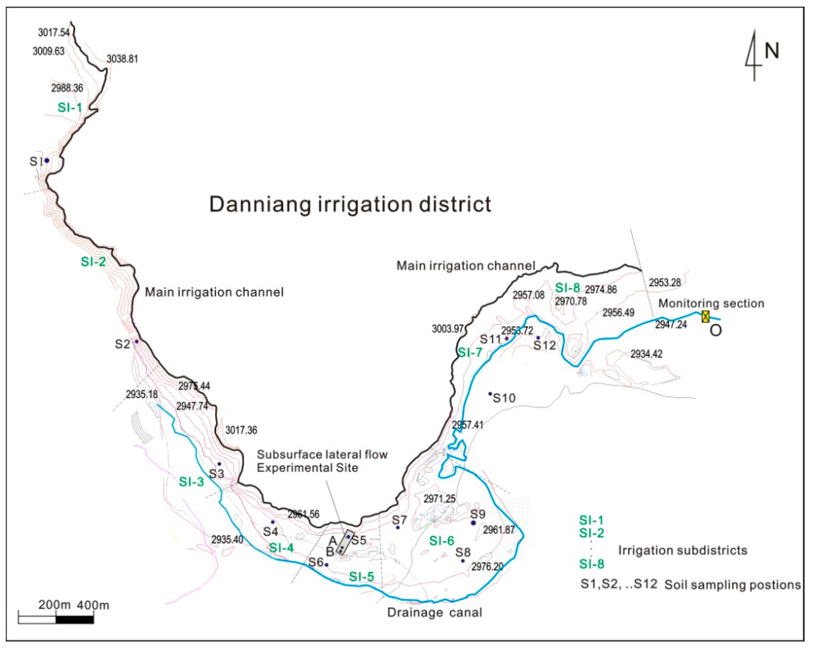
The irrigation and drainage canals in the irrigation district are shown in Figure 1. The main irrigation channel was arranged along the contour lines of the piedmont. Irrigation subdistricts 1, 2, 3, 7, and 8 were located in the long and narrow region in the piedmont and irrigated with water directly from the main irrigation channel. Subdistricts 4–6 were irrigated with water from the branch irrigation channels. The average elevation difference between the main irrigation channel and drainage canal was 3.6 m.

The soil thickness was 50 cm and underlain with a loose rock layer comprised of coarse sand and rubble 2–40 cm in size. The soil was classified as dark brown soil according to the standards of the second national soil survey in China and sandy loam according to the standards of the US Department of Agriculture (UNSADO). The rock layer was more than 20 m thick. Samples were taken at 12 locations (Figure 1) to determine soil physical parameters (

Table 1. Soil physical properties.

Depth (cm)	Clay (%)		Sand (%)		Silt (%)		Bulk Density (g/cm3)
	Mean ± STD a	Max/Min b	Mean ± STD	Max/Min	Mean ± STD	Max/Min	Max/Min
0–10	12.4 ± 4.3	17.3/10.6	53.6 ± 2.3	55.4/47.0	24.7 ± 4.6	28.6/16.4	0.98/1.32
20–30	12.9 ± 9.6	20.4/10.1	55.0 ± 8.7	57.9/47.4	27.1 ± 0.9	30.0/22.0	1.20/1.42
30–40	10.4 ± 7.7	14.8/9.4	52.3 ± 4.1	61.3/48.2	27.3 ± 3.9	31.0/23.0	1.24/1.48
40–50	11.8 ± 6.3	19.4/7.3	52.4 ± 3.6	54.9/45.6	27.8 ± 5.6	33.8/21.5	1.22/1.38
50+	0	0	100.0 ± 0.0	100/100	0	0	1.36/1.40

^a Value of mean and standard deviation; ^b Maximum and minimum values.

). Fertilization was performed twice with a dose of 18,000.0 and 6000.0 kg urea/km² for the first and second irrigation, respectively.

2.2. Monitoring Hydrological and ANPS Pollution Transport and Transformation Processes in the Soil and Rock

Soil samples were taken in different layers (each 10 cm thick) from 0–50 cm depth during the growing period of highland barley. In each sampling event, the samples were obtained at 12 locations to determine soil water content and concentrations of the major ANPS nitrogen pollutants (i.e., NH₄⁺-N and NO₃⁻-N). All soil samples were collected using a cutting ring with a volume of 100 cm³. Fourteen and fifteen sampling events were conducted during the growing period of highland barley in 2014 and 2015, respectively. The soil water content and NH₄⁺-N and NO₃⁻-N concentrations in these samples were measured at the Farmland Water Conservancy Laboratory of the Tibet Agriculture and Animal Husbandry College.

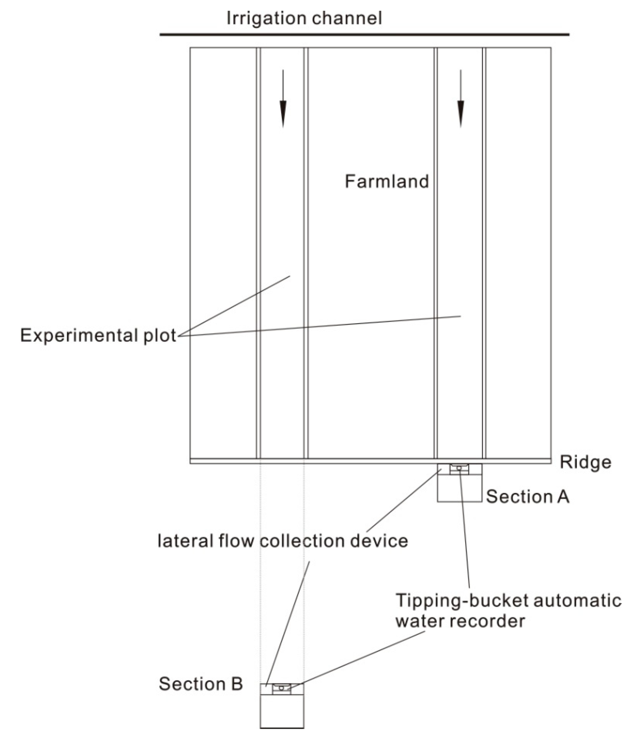
A subsurface lateral flow experimental site was constructed in the irrigation district (Figure 1) to measure subsurface lateral flow and nitrogen transport and transformation processes in the rock (Figure 2). Two 78-m long and 2-m wide experimental plots were set up. The plot length was identical to those of ridged fields in the irrigation district. The borders of the experiment plot were isolated with steel plates compressed into the ground to a depth of 20 cm. A 0.5-m wide protected area was set outside the steel plates, wherein steel plates were arranged in parallel to the experimental plots. Two subsurface lateral flow monitoring sections (A and B) were set at 0.5 m and 20.0 m, respectively, behind the ridge of plots. A trench (5.0 m long and 2.0 m wide) was excavated mechanically to a depth of 4.0 m. Subsurface lateral flow collection devices were set at a depth of 3 m below the soil. The collection device was compressed into the rock to a depth of 20 cm. A tipping-bucket automatic water recorder was introduced to measure subsurface lateral flow rate. The bucket had a volume of 50 mL and was automatically tipped after being filled. The time and frequency of tipping were automatically recorded, enabling automatic monitoring of the subsurface lateral flow rate. Meanwhile, water samples were collected to measure NH₄⁺-N and NO₃⁻-N concentrations. The area between sections A and B was covered with a rainproof film to prevent water infiltration into the soil. The amount of irrigation in the experimental site was identical to that in the field during the growing period of highland barley.

The kinetic coefficients of pollutant transformation were determined based on the mass balance method [27,28]. Undisturbed rock samples were collected using a stainless-steel sleeve (10 cm long and 5 cm in diameter). Ion exchange resins were placed at the bottom and top of the steel sleeve to eliminate the effects of the in- and out-fluxes of pollutants at the border on the measurement of the transformation process. The steel sleeve was returned to the sampling point with backfilling. The samples were retrieved 7 days later. The NH₄⁺-N and NO₃⁻-N concentrations were measured on the sampling day and 7 days later. The mass difference was taken as the amount of pollutant transformation. Samples were taken at three positions in the soil layer (10–40 cm depth) and loose rock layer (70–90 cm depth). The measurements were made twice, three times, and once, respectively, during the sowing–tilling, jointing–heading, and flowering–filling stages of the highland barley.

A monitoring section, i.e., section O in Figure 1, was set at the outlet of the surface drainage canal in the irrigation district. The drainage process was monitored automatically using a Doppler flowmeter, and water samples were taken to measure NH₄⁺-N and NO₃⁻-N concentrations in the surface drainage.

Meteorological parameters, including radiation, temperature, humidity, wind speed, and air pressure, were measured at a meteorological station within the study area.

2.3. Simulation of Hydrological and ANPS Pollution Transport Processes in the Plateau Irrigation District

Water flow and transport processes were simulated independently in the irrigation subdistricts with different parameters related to the irrigation events and size of the irrigation subdistrict. The flow and pollution fluxes at the outlet of the drainage canal represent the confluence and superposition processes of flow discharged from the rock, including from subsurface lateral flow and groundwater.

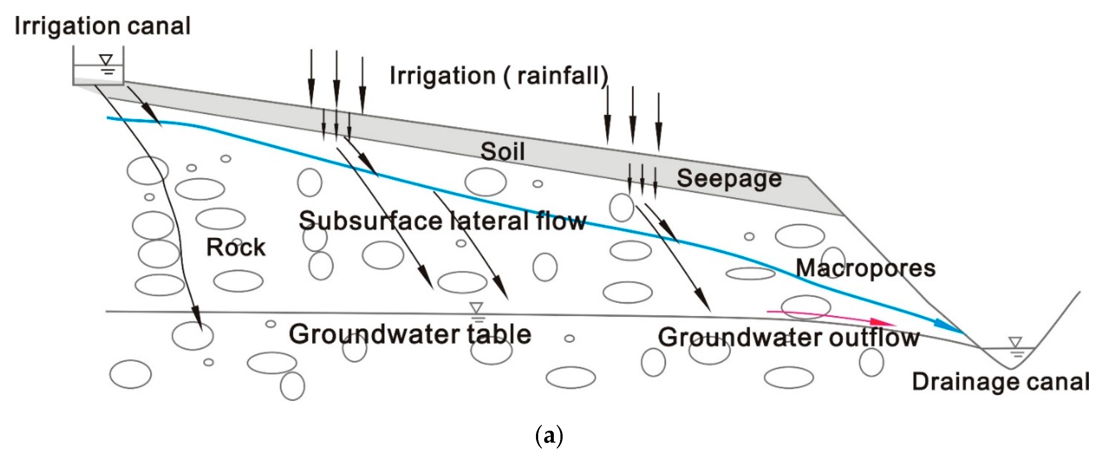
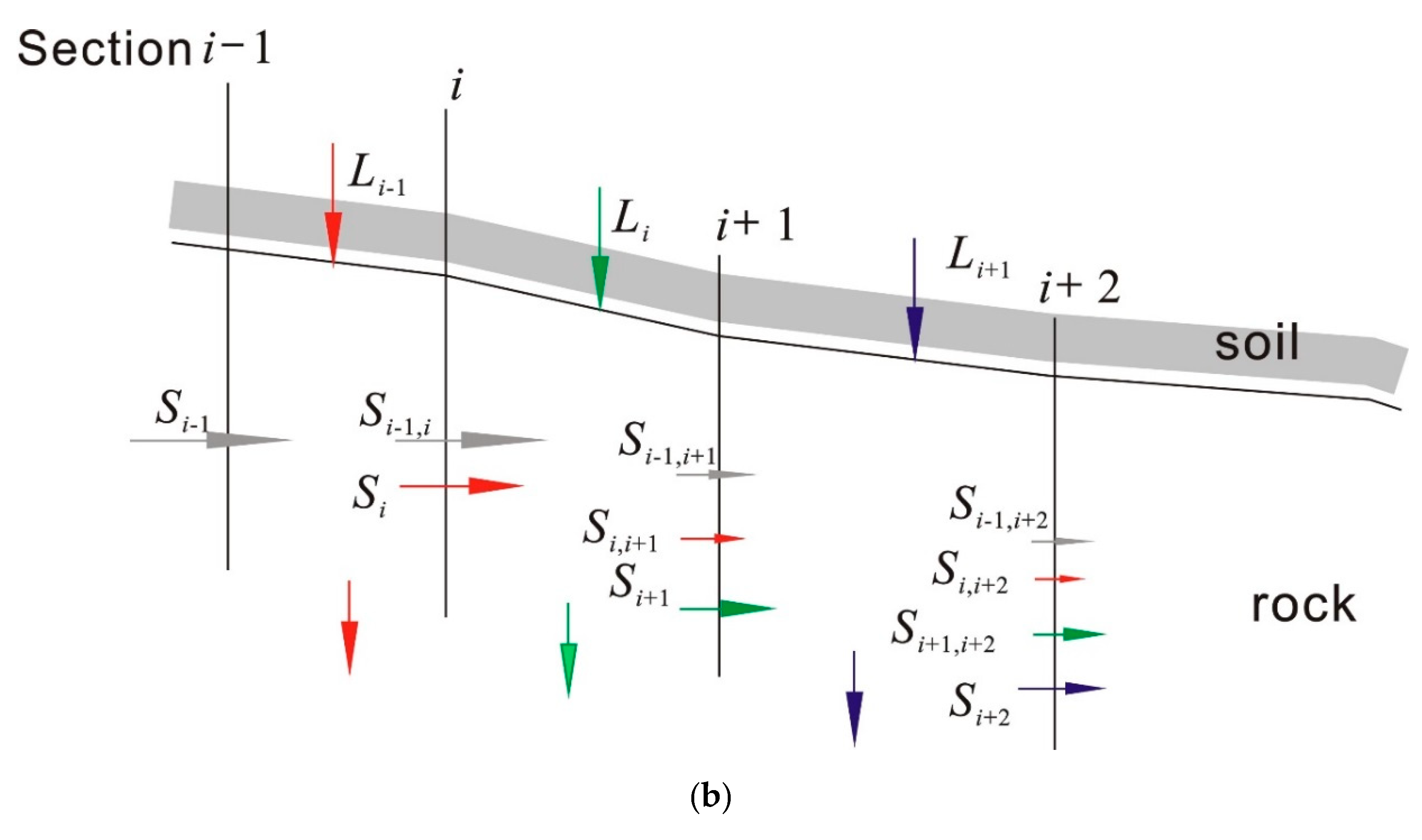
Subsurface lateral flow in the rock is illustrated in Figure 3. Monitoring data from 2014 and 2015 showed that no significant surface runoff occurred during irrigation. A stepwise method was used to describe subsurface lateral flow processes in the rock. In the interval from i to i + 1, the deep seepage flux L_i that enters the rock from the soil can be expressed as

$$L_i=I-\Delta W_i$$

(1)

where I is the amount of irrigation (or rainfall) and $\Delta W_i$ is the variation of soil water content before and after irrigation (or rainfall).

The flux L_i seeps into the rock from the soil and moves laterally toward to the surface drainage canal as well as vertically into the groundwater. The lateral inflow flux from soil seepage L_{i − 1} at section i is denoted as S_i (Figure 3b). In the interval from section i to section i + 1, only a partial flux of S_i continuously moves to the surface drainage canal due to high arbitrariness of flow in the loose fractured rock.

$$S_{i,i+1}=S_i\mu (G)$$

(2)

A subsection-fitting method was used for the calculation of the subsurface lateral flow coefficient $\mu (G)$ in the rock [29]:

$$\mu (G)=\alpha e^{-\beta t}\sqrt{t}$$

(3)

where t is the relative time (seepage time/irrigation duration) and α and β are parameters related to the rock structure.

At section i + 1, the lateral flow flux S_i decreases to S_i,i+1. The flux at section i + 1 also includes lateral flow from soil seepage L_i, denoted as flux S_{i + 1}. At section i, the lateral flux to the surface drainage canal is the superposition of all fluxes and can be expressed as

$$S={\displaystyle \sum _{j=0}^m{S}_{i-j,i}}$$

(4)

In the rock, the impact of the diffusion process on pollutant migration can be ignored in the case of a long flow path, and the convection (i.e., the product of water flux and pollution concentration) process can be used to describe the pollutant transport flux. The mean values of the measured soil water content and NH₄⁺-N and NO₃⁻-N concentrations in the soil profile were used as inputs in the subsurface lateral flow and transport simulation.

The amount of seepage water from the rock to the aquifer in the section from i to i + 1 is

$$w{r}_{i,i+1}=S_i(1-\mu (G))$$

(5)

Assuming that variations in groundwater flow are linearly related to the rate of change in water table height, we obtain

$$\frac{d{Q}_{gwi,i+1}}{dt}=\frac{K_s}{\mu {L_g}^2}(w{r}_{i,i+1}-Q_{gwi,i+1})$$

(6)

where Q_{gwi,i + 1} is the groundwater flow into the surface drainage canal, $\mu$ is the specific yield of the shallow aquifer (cm³/cm³), and L_g is the distance from the ridge of the groundwater to the surface drainage canal. Water flow and pollutant transport processes in the drainage canal can be characterized by the following Equations:

$$\frac{\partial A}{\partial t}+\frac{\partial \left(Q^2/A\right)}{\partial x}+gA\left(\frac{\partial h}{\partial x}-i_0+i_f\right)=q$$

(7)

$$Q=\frac{A}{n}{R}^{2/3}{i}_f^{1/2}$$

(8)

where A is the area of the drainage canal cross section; Q is the surface drainage flow rate; q is the inflow during the calculation period (as determined using Equations (4) and (6)); h is the depth of the drainage channel; n is the Manning roughness coefficient; R and i₀ are the hydraulic radius and longitudinal slope of the drainage channel, respectively; and i_f is the friction slope. Due to the prevention of field ridges and the high soil permeability in the irrigation zone, irrigation and rainfall did not typically produce runoff.

The transformation processes in the rock and drainage water were described using the first-order kinetics described by Equation [9]:

$$c_{t+1}=c_t{e}^{-kt}$$

(9)

where c_t and c_t+1 are the concentrations of pollutants (NH₄⁺-N or NO₃⁻-N) at times t and t + 1 (mg/L). The k is a lump factor to quantify pollutant transformation caused by various physical, chemical, and biological processes in the rock or in the drainage water (day⁻¹).

2.4. Calibration of Model Parameters

Monitored flow rates and NH₄⁺-N and NO₃⁻-N concentration at sections A and B in the rock and at the outlet of the drainage canal during the highland barley growing period in 2014 were used to calibrate model parameters. The objective function was defined as

$$\Phi \left([b]\right)={\displaystyle \sum _{j=1}^{m_q}{v}_j{\displaystyle \sum _{i=1}^{n_{qj}}{\left({g_j}^{*}(x,t_i)-g_j(x,t,[b]\right)}^2}}$$

(10)

where m_q is the number of monitoring variables (flow rate, NH₄⁺-N concentration, and NO₃⁻-N concentration), n_qj is the monitoring number of variable j, ${g_j}^{*}(x,t_i)$ is the monitored value of variable j at time t_i in the monitoring position, and $g_j(x,t_i,[b])$ is the result of using optimized parameter [b]. Additionally, v_j is the weight of variable j, which is used to reduce the magnitude effect of different variables and different monitoring events on the calculated results.

$$v_j=\frac{1}{n_j{\sigma }_j}$$

(11)

where ${\sigma }_j$ is the standard deviation of the monitored value for variable j.

The simulation results of the NH₄⁺-N and NO₃^--N concentrations were evaluated using four indicators: the Nash–Sutcliffe coefficient (NSE) [30], the relative root mean square error (rRMSE), the fraction bias (F_B), and the fractional gross error (F_E) [31]; NSE, F_B, and F_E are calculated as follows:

$$NSE=1-\frac{{\displaystyle \sum _{t=1}^n{(O_t-P_t)}^2}}{{\displaystyle \sum _{i=1}^n{(O_t-\stackrel{\_}{O})}^2}}$$

(12)

$$F_B=\frac{1}{n}{\displaystyle \sum _{i=1}^n\frac{P_t-O_t}{(P_t+O_t)/2}}$$

(13)

$$F_E=\frac{1}{n}{\displaystyle \sum _{i=1}^n\frac{\left|P_t-O_t\right|}{(P_t+O_t)/2}}$$

(14)

where O_t and P_t are the monitored and calculated values at time t, respectively, $\overline{O}$ is the mean of the monitored value, and n is the number of observation points. The ideal value of NSE was 1. F_B and F_E were used to describe the systematic error and total deviation between the observed and simulated values, respectively.

2.5. Sobol’s Sensitivity Analysis

The effects of input parameters on model performance are evaluated using Sobol’s method. The model can be represented in the following functional form:

$$Y=f(X)=f(x_1,x_2...x_n)$$

(15)

where Y is the model output and X = (x₁, x₂,…x_n) is the parameter and physical variable set. For all of parameters and physical variables used in the model, two low-discrepancy random sequences are generated using the random sampling method [32].

$$M_A=\left[\begin{array}{cccc}{x}_{11}& x_{12}& \cdots & x_{1n}\\ x_{21}& x_{22}& \cdots & x_{2n}\\ ⋮& ⋮& ⋮& ⋮\\ x_{m1}& x_{m2}& \cdots & x_{mn}\end{array}\right]\hspace{1em}{M}_B=\left[\begin{array}{cccc}{x}_{11}^{\prime }& x_{12}^{\prime }& \cdots & x_{1n}^{\prime }\\ x_{21}^{\prime }& x_{21}^{\prime }& \cdots & x_{2n}^{\prime }\\ ⋮& ⋮& ⋮& ⋮\\ x_{m1}^{\prime }& x_{m2}^{\prime }& \cdots & x_{mn}^{\prime }\end{array}\right]$$

(16)

where m is the sampling repetition and n is the number of parameters. A new matrix was formed by replacing the parameters in the ith column in matrix B (i.e., sample values of parameter x_i) with the ith column data in matrix A.

Finally, matrices A and B were stacked into one “combined” matrix, C, which has n + 2 rows and n columns.

$$M_{C_i}=\left[\begin{array}{cccccc}{x}_{11}& x_{12}& \cdots & x_{1i}^{\prime }& \cdots & x_{1n}\\ x_{21}& x_{22}& \cdots & x_{2i}^{\prime }& \cdots & x_{2n}\\ ⋮& ⋮& ⋮& ⋮& ⋮& ⋮\\ x_{m1}& x_{m2}& \cdots & x_{mi}^{\prime }& \cdots & x_{mn}\end{array}\right],i=1,2\dots n$$

(17)

The first-order sensitivity index, S_i, and the total-order sensitivity index, S_Ti, were calculated as follows:

$$S_i=\frac{\frac{1}{m-1}{\displaystyle \sum _{k=1}^m{y}_B^{(k)}{y}_C^{(k)}-\frac{1}{m}{\displaystyle \sum _{k=1}^m{y}_A^{(k)}{y}_B^{(k)}}}}{V(y_A)}$$

(18)

$$S_{Ti}=1-\frac{\frac{1}{m-1}{\displaystyle \sum _{k=1}^m{y}_B^{(k)}{y}_C^{(k)}-{\left(\frac{1}{m}{\displaystyle \sum _{k=1}^m{y}_A^{(k)}}\right)}^2}}{V(y_A)}$$

(19)

where $y_A^{(k)}$, $y_B^{(k)}$, and $y_C^{(k)}$ are the model outputs with parameters in matrices A, B, and C, respectively. The variance of the output with the parameters in matrix A is calculated as

$$V(y_A)=\frac{1}{m-1}{\displaystyle \sum _{k=1}^m{\left(y_A^{(k)}-\frac{1}{m}{\displaystyle \sum _{k=1}^m{y}_A^{(k)}}\right)}^2}$$

(20)

The first-order index, S_i, is a measure of the variance contribution of the individual parameter x_i to the total model variance. The difference between the first-order sensitivity index and the total-order sensitivity index can be regarded as a measure of the interaction between parameter x_i and the other parameters.

3. Results

3.1. Characterization of Flow and NH₄⁺-N and NO₃⁻-N Transport

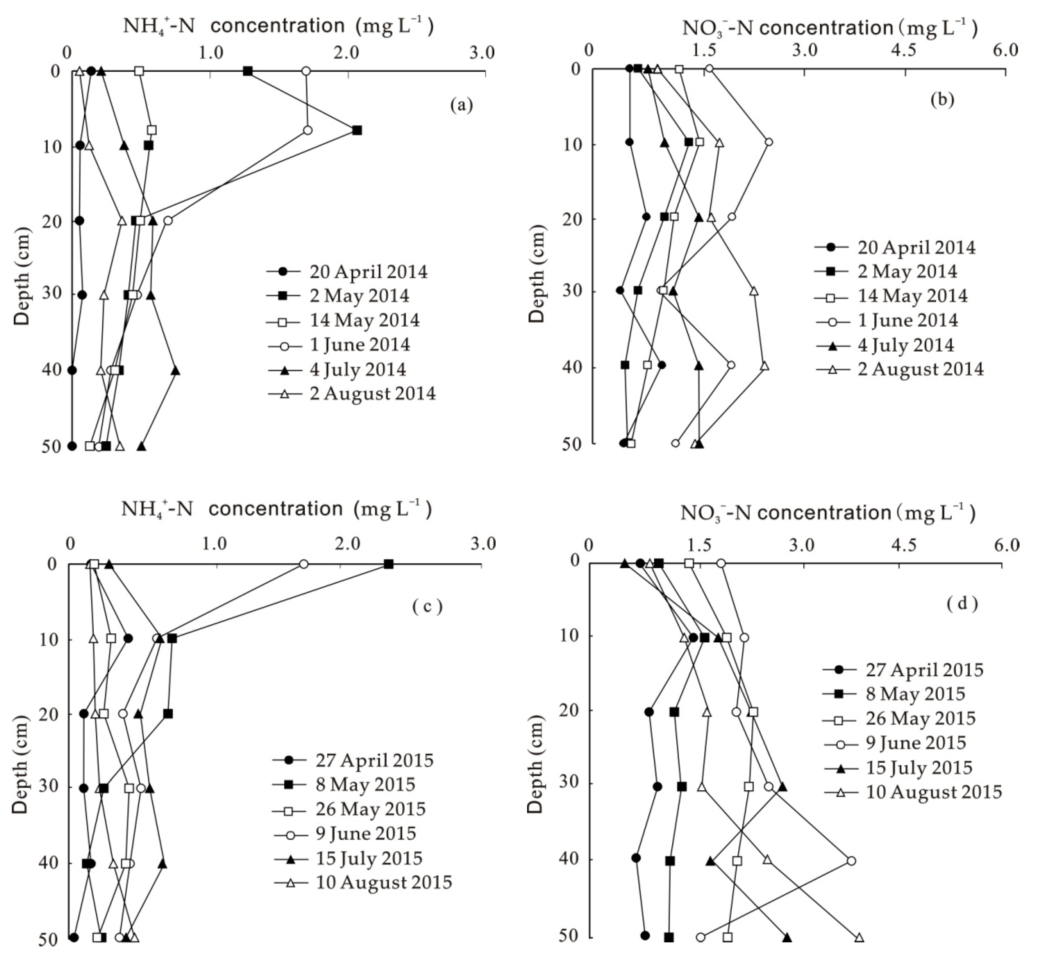
The total rainfall and irrigation were 712 mm and 863 mm for the growing period of highland barley in 2014 and 2015, respectively. Figure 4a,b shows the measured concentrations of NH₄⁺-N and NO₃⁻-N, respectively, at different depths and during the highland barley growing period of 2014. Figure 4c,d shows the same distributions for 2015. Compared with the mean NH₄⁺-N and NO₃⁻-N concentrations at different depths in 2014, the mean NH₄⁺-N concentration decreased by 14.22, 11.47, and 6.78%, respectively, and the mean NO₃⁻-N concentration decreased by 3.18, 22.4, and 17.3%, respectively, during the sowing–tilling, jointing–heading, and flowering–filling stages of 2015. Due to a 21.2% increase in rainfall and irrigation during the highland barley growing period of 2015, the mean concentrations of NH₄⁺-N and NO₃⁻-N decreased by 10.8 and 14.3%, respectively. In the bottom soil layer (40–50 cm), the peak concentrations of NH₄⁺-N and NO₃⁻-N during the highland barley growing period of 2014 were 0.86 and 4.08 mg/L, respectively, whereas for 2015, these concentrations were 0.65 and 3.76 mg/L, representing a decrease of 24.4 and 7.8%, respectively.

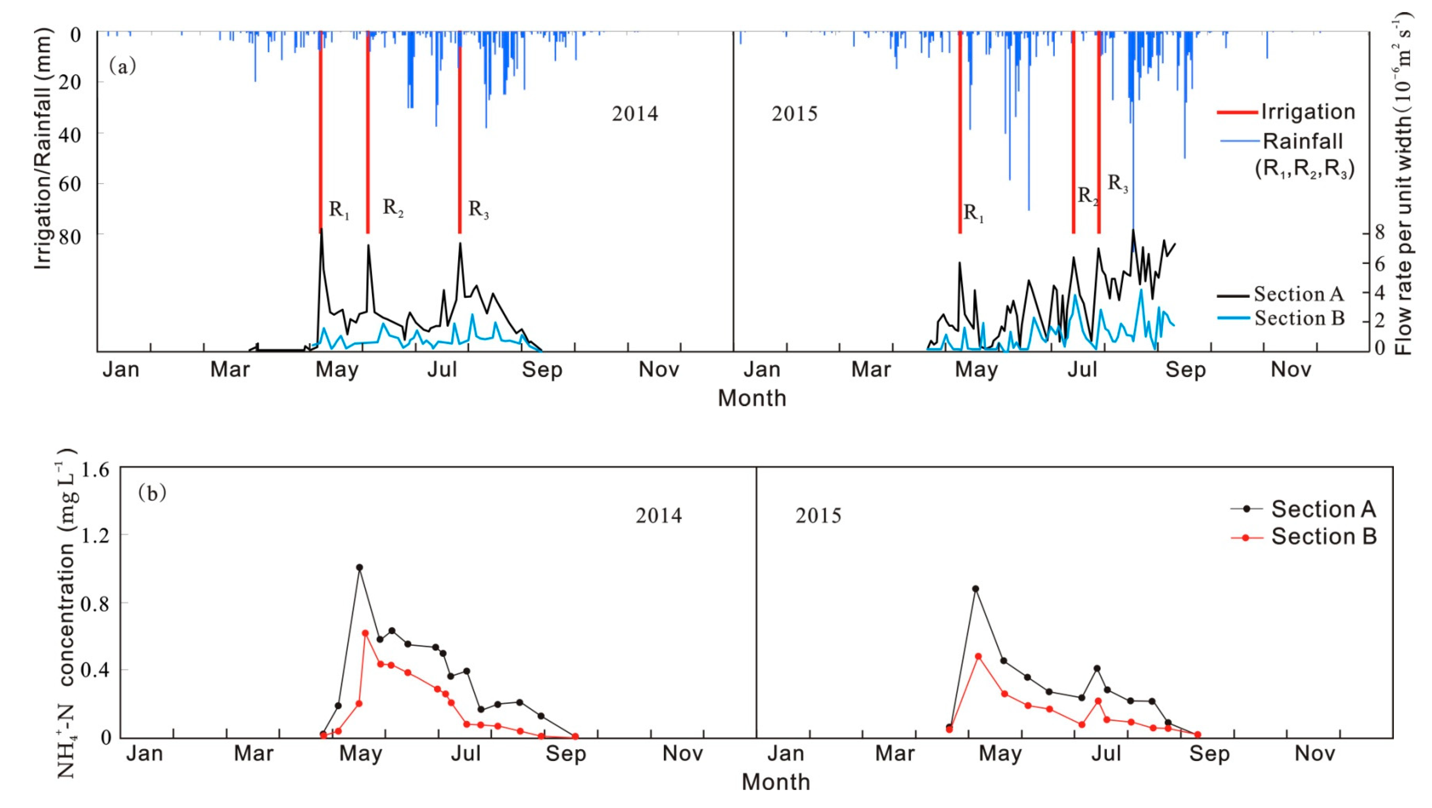
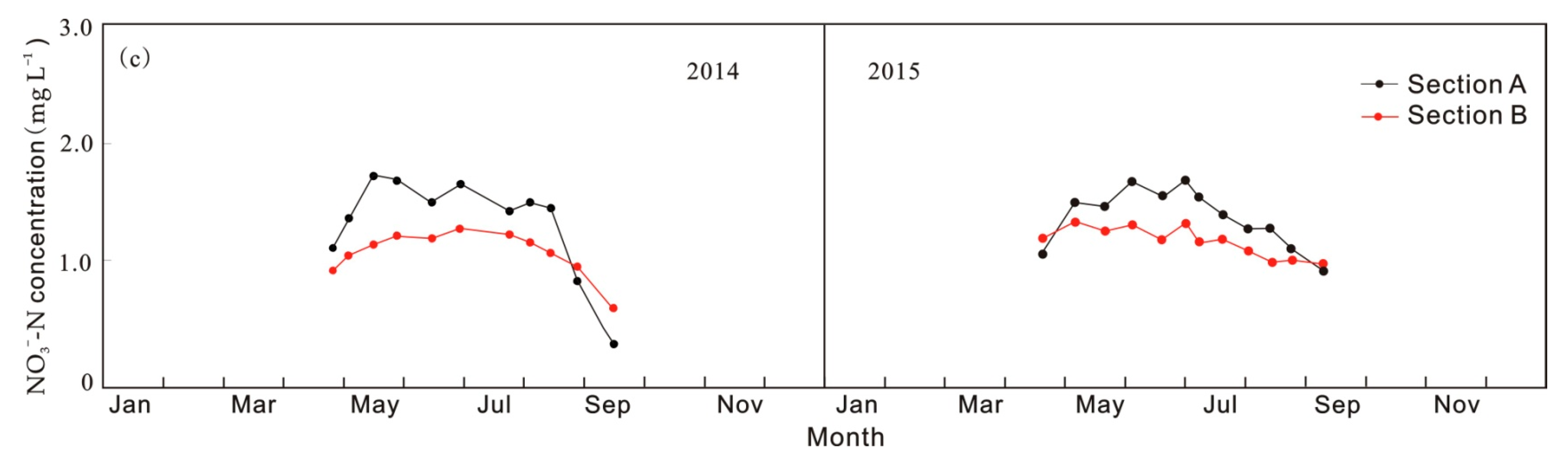
Figure 5a–c compares the rainfall and irrigation, subsurface lateral flow rate per unit width, and NH₄⁺-N and NO₃⁻-N concentrations in the subsurface lateral flow, monitored at the lateral flow experimental site during the experimental periods of 2014 and 2015.

Table 2. Comparison of NH₄⁺-N and NO₃⁻-N mass seepage flux per area (kg/s/km²) during the highland barley growing periods.

Chemical	Sowing and Tilling Stages		Jointing and Heading Stages		Flowering and Filling Stages
	Mean	Max/Min a	Mean	Max/Min	Mean	Max/Min
2014
NH4+-N	6.14 × 10−6	9.78 × 10−5/3.30 × 10−6	4.24 × 10−6	1.01 × 10−4/1.77 × 10−6	2.11 × 10−6	8.94 × 10−6/1.57 × 10−6
NO3−-N	3.25 × 10−6	5.14 × 10−5/1.07 × 10−6	3.44 × 10−5	5.78 × 10−4/1.21 × 10−5	8.60 × 10−6	1.84 × 10−5/3.39 × 10−6
2015
NH4+-N	7.44 × 10−6	1.26 × 10−4/0.54 × 10−6	3.99 × 10−6	7.93 × 10−5/1.15 × 10−6	2.02 × 10−6	4.64 × 10−6/1.33 × 10−6
NO3−-N	3.18 × 10−6	8.74 × 10−5/2.21 × 10−6	4.04 × 10−5	6.48 × 10−4/2.04 × 10−5	7.54 × 10−5	1.02 × 10−4/5.48 × 10−5

^a Maximum and minimum values.

compares the deep seepage fluxes of NH₄⁺-N and NO₃⁻-N measured during each growth stage. For the three irrigation events in 2014 (Figure 5a), the amount of seepage water entering the rock through the soil accounted for 37.4, 36.6, and 41.2% of the irrigation, respectively. For 2015, seepage accounted for 40.2, 45.3, and 39.4% of the irrigation, respectively. Seepage due to rainfall accounted for 0 to 52.4% of total rainfall in two years.

The peak concentration of NH₄⁺-N in subsurface lateral flow appeared after fertilization in both 2014 and 2015. Compared with the flow rate and NH₄⁺-N and NO₃⁻-N concentrations at Section A in 2014, the mean value of the flow rate and NH₄⁺-N and NO₃⁻-N concentrations at Section B decreased by 34.2, 54.8, and 44.6%, respectively, and the peak values decreased by 82.4, 44.2, and 38.7%, respectively. With increased rainfall and irrigation in 2015, the difference in flow rate and pollution concentrations between Section A and B decreased; the mean value of the flow rate and NH₄⁺-N and NO₃⁻-N concentrations at position B decreased by 24.2, 34.5, and 28.7%, respectively, and the peak values decreased by 74.4, 24.2, and 14.7%, respectively.

3.2. Simulation of ANPS Pollutant Transport and Transformation Processes

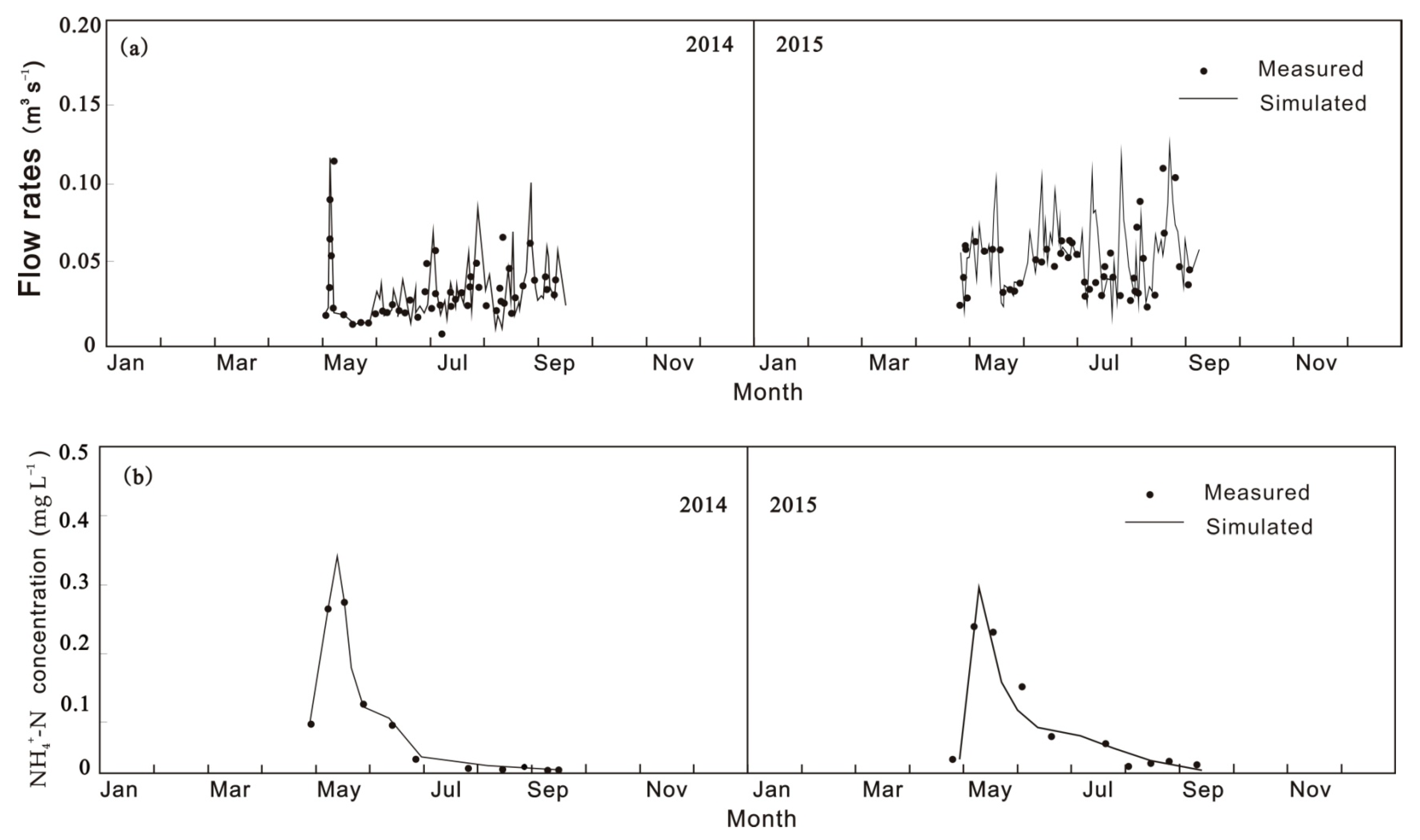
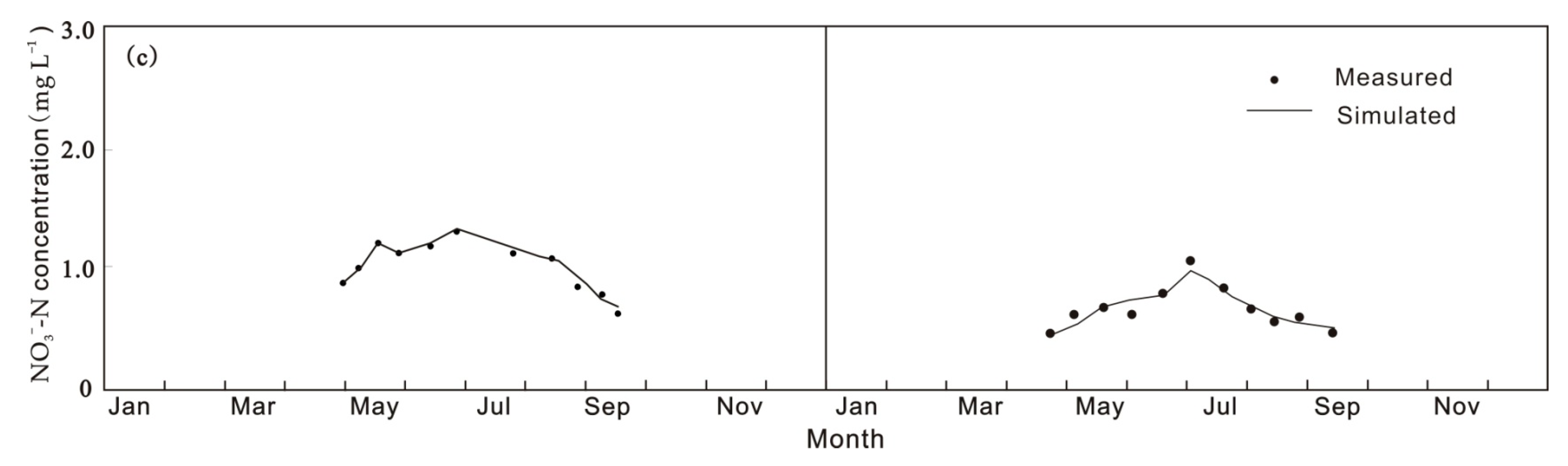
The calibrated parameters are listed in

Table 3. Parameter and physical variable list.

No.	Brief Description (Unit)	Calibrated	Minimum	Maximum
1	Seepage from soil into rock (mm day−1), LE	-a	1.4	12.6
2	NH4+-N concentration in the soil water(mg L−1)	-	0.4	6.2
3	NO3−-N concentration in the soil water(mg L−1)	-	1.8	8.4
4	α, parameter in Equation (3)	1.554	1.00	2.05
5	β, parameter in Equation (3)	0.0182	0.0020	0.110
6	NH4+-N transformation rate in the lateral flow in the rock (day−1)	0.142	0.102	0.20
7	NO3−-N transformation rate in the lateral flow in the rock (day−1)	0.171	0.144	0.224
8	Ksat, parameter in Equation (6) (m s−1)	3.42 × 10−5	3.08 × 10−5	3.94 × 10−5
9	µ, parameter in Equation (6)	0.15	0.12	0.18
10	L, parameter in Equation (6) (m)	240	200	280
11	NH4+-N transformation rate in the surface drainage (day−1)	0.11	0.09	0.14
12	NO3−-N transformation rate in the surface drainage (day−1)	0.09	0.06	0.13

^a Measured data were used.

. Figure 6a–c compares the simulated and measured flow rate and NH₄⁺-N and NO₃⁻-N concentrations at the outlet (Section O) of the surface drainage canal.

The accuracy of calculated flow and transport processes from soil to the outlet of the drainage canal was quantified with the indexes of NSE, rRMSE, F_E, and F_B listed in

Table 4. Indexes to quantify the accuracy of the simulated flow and transport processes ^a.

Flow rate and Chemical Concentrations	NSE	rRMSE (%)	FE	FB
Flow rate	0.791	5.132	0.2014	0.031
NH4+-N concentration	0.701	8.364	0.2466	0.048
NO3−-N concentration	0.644	7.532	0.3172	−0.051

^aNSE, rRMSE, F_E, and F_B denote the Nash–Sutcliffe efficiency, relative root mean square error, fraction bias, and fractional gross error, respectively.

. The NSE value exceeded 0.6. The F_B remained less than 15% throughout the growing period of highland barley, demonstrating no systematic error between the simulated and measured results. F_B and F_E indexes of the simulated values were within the range of ±0.15/0.3 (F_B/F_E), indicating high accuracy of the simulation [31]. All the results of the Nash–Sutcliffe coefficient, rRMSE, and F_E demonstrate that the model can effectively describe the transport and transformation processes of pollutants in the rock and estimate the pollution load accurately in this plateau irrigation area.

Table 5. Mass balance of non-point source pollution types during the highland barley growing periods.

Growing Stages	Water (104 m3 km−1)	NH4+-N Mass (kg km−1 )			NO3−-N Mass (kg km−1)
		Seepage	Transformation	Discharge	Seepage	Transformation	Discharge
Sowing and tilling stages	2.16	2.550	5.71	7.74	43.8	4.91	9.77
Jointing and heading stages	3.64	2.386	3.29	6.42	84.2	11.90	22.45
Flowering and filling stages	3.87	0.492	0. 64	0.98	74.5	9.77	14.42
Total	9.67	5.428	9.64	15.14	202.5	26.58	46.64

lists the mass balance of seepage water, NH₄⁺-N, and NO₃⁻-N from the soil during various stages of the highland barley growing period in 2015, which included the mass of NH₄⁺-N and NO₃⁻-N in deep seepage from the soil into the rock, the mass of NH₄⁺-N and NO₃⁻-N pollutants transformed in the rock, and the mass of NH₄⁺-N and NO₃⁻-N discharged into the surface drainage canal. Overall, 29.4% of deep seepage water was due to irrigation and rainfall discharged into the drainage channel. The transformation of NH₄⁺-N accounted for 13.0–22.4% of total NH₄⁺-N in the deep seepage, whereas NH₄⁺-N discharge into the drainage channel accounted for 19.9–30.4% of total NH₄⁺-N in the deep seepage. The transformation of NO₃⁻-N accounted for 11.2–14.1% of total NO₃⁻-N in the deep seepage, whereas NO₃⁻-N discharge into the drainage channel accounted for 19.4–26.7% of total NO₃⁻-N in the deep seepage.

3.3. Sensitivity Evaluation of Model Parameters

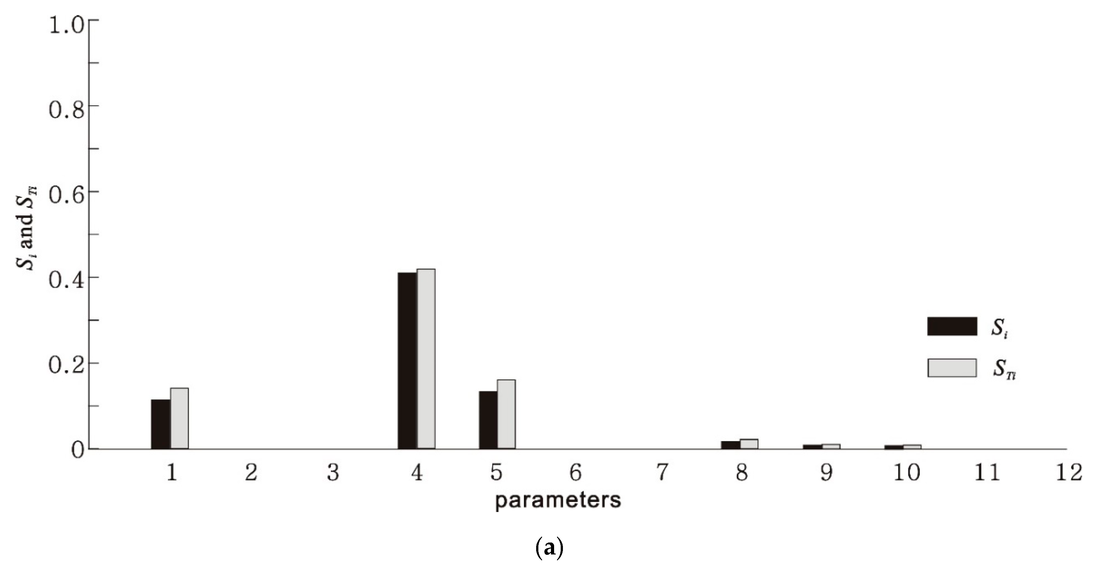
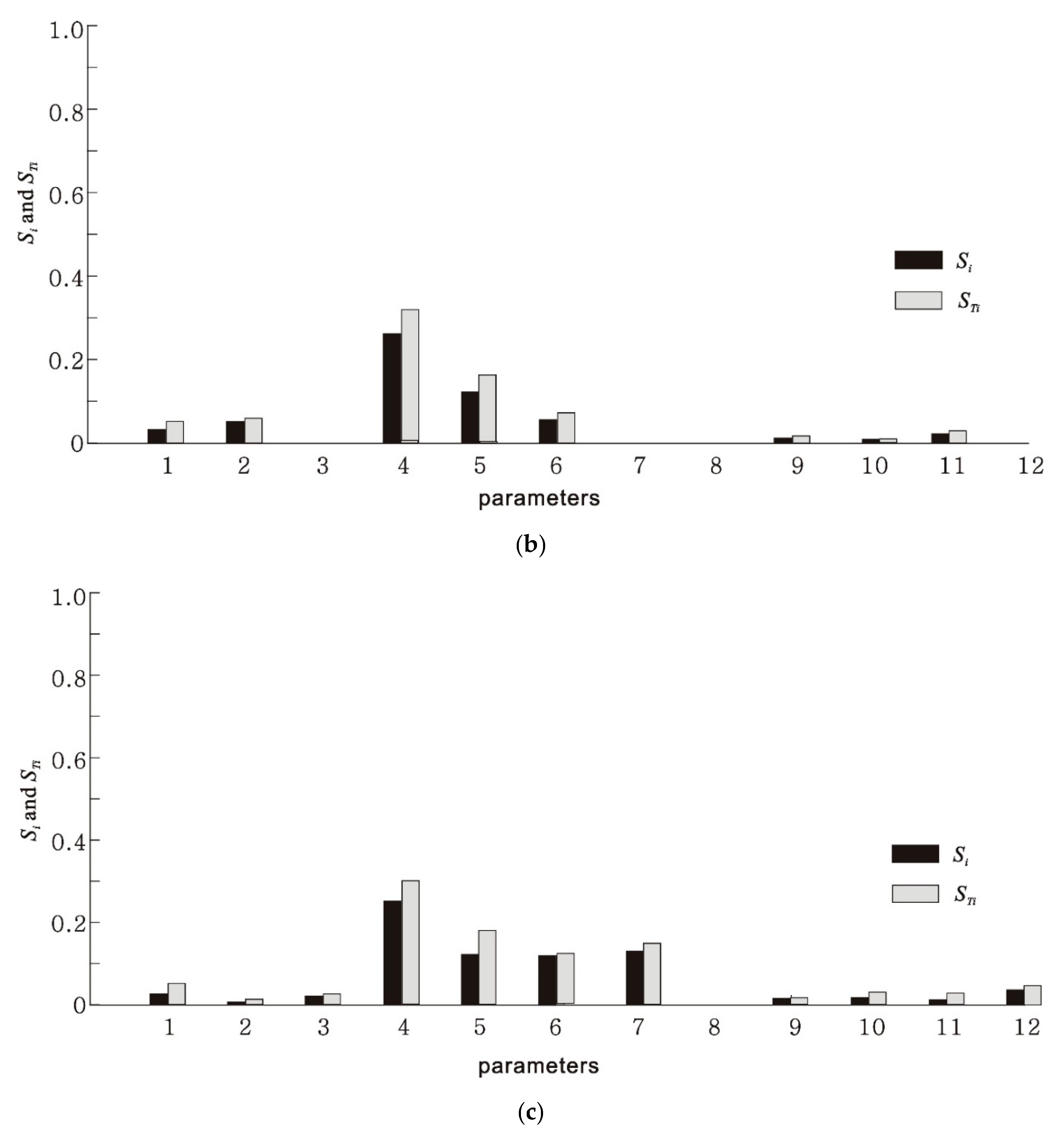
The first- and total-order sensitivity indices of 12 parameters are shown in Figure 7. The x-axis represents the parameter number listed in Table 3, and the y-axis represents the first- and total- order sensitivity indices (black and gray bars, respectively). It is noted that the sum of all first-order indices is less than 1, which means that the model is nonadditive, as expected. The first- and total- order sensitivity indices of the parameters related to subsurface lateral flow in the rock (α and β) were significantly higher than the other parameters. The first- and total-order sensitivity indices of the parameters related to groundwater discharge into surface drainage were the lowest of all parameters. These results were attributed to the lower discharge of water, NH₄⁺-N, and NO₃⁻-N from groundwater than from subsurface lateral flow.

The parameters related to subsurface lateral flow exhibited the maximum sensitivity. The value of S_i for soil NH₄⁺-N concentration was higher than the rates of deep seepage from the soil into the rock. The difference in S_i and S_Ti values for the NH₄⁺-N transformation coefficient in lateral transport and surface drainage transport was significantly higher than the differences between other parameters. The results also showed that 65.2% of the variations in the simulated NH₄⁺-N concentrations at the surface drainage outlet were caused by variations of α and β in Equation (3) and 18.4% of the variations were attributed to the transformation of NH₄⁺-N. Although the values of α and β in Equation (3) were the most sensitive parameters in the NO₃⁻-N transport simulation, the values decreased by 45.2 and 27.2% compared to the values of α and β in the flow and NH₄⁺-N simulations, respectively. The sensitivity of NO₃⁻-N concentrations in the soil was also lower than that of NH₄⁺-N concentrations in the soil.

4. Discussion

In the Danniang irrigation district, the experiment results indicated that NH₄⁺-N and NO₃⁻-N concentrations are directly affected by the subsurface lateral flow process. The NH₄⁺-N and NO₃⁻-N leaching per unit rainfall and irrigation were 4.25 and 18.45 kg km⁻² mm⁻¹, and the ratio of the total N leaching to the fertilizer N application was 0.34. These results were substantially different with those of Ju and Zhang [33], who reported that the N leaching in hilly barley crop land was in the range of 1.05 × 10⁻² to 1.18 kg km⁻² mm⁻¹, and the ratio of the N leaching to the fertilizer N application was in the range of 0.044 to 0.249. The thin soil layer, irregularities in rainfall distribution, and heavy irrigation attributed to the higher N leaching in the Danniang irrigation district, especially the NH₄⁺-N leaching, was mainly attributed to heavy irrigation because fertilizer N was applied during the first and second irrigation and soil NH₄⁺-N concentrations were maintained at high levels after fertilization. In total, 45.8 kg km⁻² of NH₄⁺-N, or 84.7% of total NH₄⁺-N leaching, was caused by the irrigation. Given that the soil thickness is sufficient, the spatial and temporal distribution of NO₃⁻-N in the soil profile may be significantly changed by fertilization, irrigation, and precipitation events [34,35]. NH₄⁺-N can be converted to NO₃⁻-N rapidly under favorable water and heat conditions. As a result, less NH₄⁺-N leaching occurs [36]. In the studied irrigation district, 28.7 and 72.3% of the total NO₃⁻-N leaching was caused by irrigation and rainfall, respectively, due to the thin and highly permeable soil.

Although the mean value of the flow rates and NH₄⁺-N and NO₃⁻-N concentrations at the outlet of the drainage canal were accurately simulated, the coefficient of variation (the ratio of standard deviation to mean) of flow rates and NH₄⁺-N and NO₃⁻-N concentrations were overestimated. Due to a 21.2% increase in total rainfall and irrigation in 2015, the monitored coefficients of variation of the flow rate and NH₄⁺-N and NO₃⁻-N concentrations at the outlet of the drainage canal increased by 15.7, 18.9, and 8.2%, respectively, while the simulated increase of the coefficients of variation were 24.2, 28.4, and 10.8%, respectively. The deviations between the measured and the simulated flow rates and NH₄⁺-N and NO₃⁻-N concentrations might be attributed to using the lumping factor to characterize the various flow and transformation processes. The storage effect and the nonlinear flow processes in the rock also affected the accuracy of the calculated concentrations. As shown in Figure 6, the flow rates simulated with the calibrated parameters were lower than the values measured in July 2015. The mean values of the measured and simulated flow rates were 0.0338 and 0.0402 m³/s, respectively, at the outlet of the drainage canal. Soil seepage into the rock was significantly reduced because rainfall was only 14.5 mm in June 2015 (Figure 4), and part of the seepage was stored in fractures and pores in the rock instead of being discharged into the surface drainage canal. As a result, the model underestimated flow rates and overestimated NH₄⁺-N and NO₃⁻-N concentrations by 4.71 and 5.64%, respectively, for this period.

The parameters of the dominant flow processes, i.e., the subsurface lateral flow process, have the most first- and total-order sensitivities. This result is similar to those found at natural basins, in which the runoff is the dominant flow process and related parameters have the most first- and total-order sensitivities [25,27,37,38]. The differences between the first- and total-order sensitivity indices of the parameters used to describe subsurface lateral flow process were significantly less than those for the parameters used in simulating the dominant flow process in the watershed, since the range of flow velocity in the rock was limited and fewer factors caused variation in the subsurface lateral flow. There were two parameters, i.e., α and β, in Equation (3) that were sensitive to the both subsurface lateral flow and nitrogen (NH₄⁺-N and NO₃⁻-N) transport and transformation processes. The Sobol’s sensitivity indices of α were significantly greater than the indices of β for the flow process, whereas the indices of α decreased and the indices of β increased for the nitrogen transport and transformation processes. The result showed that the peak flow rate after rainfall or irrigation has more influence on the estimation of flow process, and the description of the nonlinear subsurface flow process was more influential on the simulated output of the NH₄⁺-N and NO₃⁻-N concentrations.

5. Conclusions

Field experiments were conducted to investigate the hydrology and ANPS transport and transformation processes in the Danniang irrigation region, Tibet, during the highland barley growing periods in 2014 and 2015. A distributed model was constructed to simulate flow and ANPS (NH₄⁺-N and NO₃⁻-N) transport and transformation from the soil to the outlet of the surface drainage canal. Water flow and transport processes were simulated in irrigation subdistricts with different parameters related to the irrigation events and the size of the irrigation subdistricts. A stepwise method was used to describe subsurface lateral flow in the rock. The flow and pollution fluxes at the outlet of the drainage canal represented the confluence and superposition processes of flow discharged from the rock, including subsurface lateral flow and groundwater.

The simulated values of flow rate, NH₄⁺-N concentration, and NO₃⁻-N concentration exhibited systematic deviations of less than 15%. Across the growing period of highland barley, the mean values of the Nash–Sutcliffe coefficient, rRMSE, the fraction bias, and the fractional gross error between the simulated and observed flow rates and NH₄⁺-N and NO₃⁻-N concentrations at the outlet of the surface drainage canal were 0.712, 7.01%, 0.04, and 0.255, respectively. These indicate that the proposed method can effectively simulate the hydrological and ANPS pollutant migration processes in this plateau irrigation district. As a result of the 21.2% increase in the rainfall and irrigation amount during the highland barley growing period in 2015, the average NH₄⁺-N and NO₃⁻-N concentrations in the soil layer decreased by 10.8 and 14.3%, respectively, due to increased deep seepage. Deep seepage due to rainfall accounted for 0–52.4% of all rainfall, whereas deep seepage due to irrigation accounted for 36.6–45.3% of all irrigation. NH₄⁺-N and NO₃⁻-N discharge into the drainage channel represented 19.9–30.4% and 19.4–26.7% of the deep seepage, respectively. Parameters in the subsurface lateral flow simulation were shown to have the most important first-order and total-order effects on the simulated flow and NH₄⁺-N and NO₃⁻-N concentrations at the outlet of the surface drainage canal.

References

- Ibrikci, H.; Cetin, M.; Karnez, E.; Flügel, W.A.; Ryan, J. Irrigation-induced nitrate losses assessed in a Mediterranean irrigation district. Agric. Water Manag. 2015, 148, 223–231. [Google Scholar] [CrossRef]
- Jiménez-Aguirre, M.T.; Isidoro, D. Hydrosaline Balance in and Nitrogen Loads from an irrigation district before and after modernization. Agric. Water Manag. 2018, 208, 163–175. [Google Scholar] [CrossRef]
- Wang, K.; Zhang, R.; Chen, H. Drainage-process analyses for agricultural non-point-source pollution from irrigated paddy systems. J. Irrig. Drain. Eng.-ASCE 2014, 15, 1943–4774. [Google Scholar] [CrossRef]
- Ogden, F.L.; Julien, P.Y. CASC2D: A two-dimensional, physically based, Hortonian hydrologic model. In Mathematical Models of Small Watershed Hydrology and Applications; Singh, V.P., Frevert, D.K., Eds.; Water Resources Publications: Highlands Ranch, CO, USA, 2002; Chapter 4; pp. 69–112. [Google Scholar]
- Borah, D.K.; Xia, R.J.; Bera, M. DWSM—A Dynamic Watershed Simulation Model. In Mathematical Models of Small Watershed Hydrology & Applications; Water Resources Publications: Highlands Ranch, CO, USA, 2002; pp. 113–166. [Google Scholar]
- Neitsch, S.L.; Arnold, J.G.; Kiniry, J.R.; Srinivasan, R.; Williams, J.R. Soil and Water Assessment Tool User’s Manual Version 2000; GSWRL Report 02-02; BRC Report 02-06; TR-192; Texas Water Resources Institute: College Station, TX, USA, 2002. [Google Scholar]
- Arnold, J.G.; Moriasi, D.N.; Gassman, P.W.; Abbaspour, K.C.; White, M.J.; Srinivasan, R.; Santhi, C.; Harmel, R.D.; van Griensven, A.; Van Liew, M.W.; et al. SWAT: Model use, calibration, and validation. Trans. ASABE 2012, 55, 1491–1508. [Google Scholar] [CrossRef]
- Čerkasova, N.; Umgiesser, G.; Ertürk, A. Development of a hydrology and water quality model for a large transboundary river watershed to investigate the impacts of climate change—A SWAT application. Ecol. Eng. 2018, 124, 99–115. [Google Scholar] [CrossRef]
- Xie, X.; Cui, Y. Development and test of SWAT for modeling hydrological processes in irrigation districts with paddy rice. J. Hydrol. 2011, 396, 61–71. [Google Scholar] [CrossRef]
- Lee, S.B.; Yoon, C.G.; Jung, K.W. Comparative evaluation of runoff and water quality using HSPF and SWMM. Water Sci. Technol. 2010, 62, 1401–1409. [Google Scholar] [CrossRef]
- Chahinian, N.; Tournoud, M.G.; Perrin, J.L. Flow and nutrient transport in intermittent rivers: A modelling case-study on the Vene River using SWAT 2005. Hydrol. Sci. J. 2011, 192, 143–159. [Google Scholar] [CrossRef]
- Lucadamo, L.; De Filippis, A.; Mezzotero, A.; Vizza, S.; Gallo, L. Biological and chemical monitoring of some major Calabrian (Italy) Rivers. Environ. Monit. Assess. 2007, 146, 453–471. [Google Scholar] [CrossRef]
- Howarth, R.W. Coastal nitrogen pollution: A review of sources and trends globally and regionally. Harmful Algae 2008, 8, 14–20. [Google Scholar] [CrossRef]
- Kroeze, C.; Bouwman, L.; Seitzinger, S. Modeling global nutrient export from watersheds. Curr. Opin. Environ. Sustain. 2012, 4, 195–202. [Google Scholar] [CrossRef]
- Zhou, T.; Wu, J.; Peng, S. Assessing the effects of landscape pattern on river water quality at multiple scales: A case study of the Dongjiang River watershed. China Ecol. Indic. 2012, 23, 166–175. [Google Scholar] [CrossRef]
- Pollock, D.W.; Kookana, R.S.; Correll, R.L. Integration of the pesticide impact rating index with a geographic information system for the assessment of pesticide impact on water quality. Water Air Soil Pollut. Focus 2005, 5, 67–88. [Google Scholar] [CrossRef]
- Watanabe, T.; Kimura, M.; Asakawa, S. Dynamics of methanogenic archaeal communities based on rRNA analysis and their relation to methanogenic activity in Japanese paddy field soils. Soil Biol. Biochem. 2007, 39, 2877–2887. [Google Scholar] [CrossRef]
- Dechmi, F.; Burguete, J.; Skhiri, A. SWAT application in intensive irrigation systems: Model modification, calibration and validation. J. Hydrol. 2012, 470–471, 227–238. [Google Scholar] [CrossRef]
- Abdelwahab, O.M.M.; Ricci, G.F.; De Girolamo, A.M.; Gentile, F. Modelling soil erosion in a Mediterranean watershed: Comparison between SWAT and AnnAGNPS models. Environ. Res. 2018, 166, 363–376. [Google Scholar] [CrossRef] [PubMed]
- Belcher, K.W.; Boehm, M.M.; Fulton, M.E. Agroecosystem sustainability: A system simulation model approach. Agric. Syst. 2004, 79, 225–241. [Google Scholar] [CrossRef]
- Franceschini, S.; Tsai, C.W. Assessment of uncertainty sources in water quality modeling in the Niagara River. Adv. Water Resour. 2010, 33, 493–503. [Google Scholar] [CrossRef]
- Wang, K.; Lin, Z.; Zhang, R. Impact of phosphate mining and separation of mined materials on the hydrology and water environment of the Huangbai River basin, China. Sci. Total Environ. 2016, 543, 347–356. [Google Scholar] [CrossRef]
- Sobol, I.M. Sensitivity estimates for nonlinear mathematical models. Math. Model. Comput. Exp. 1993, 1, 407–417. [Google Scholar]
- Zhang, C.; Chu, J.; Fu, G. Sobol’s sensitivity analysis for a distributed hydrological model of Yichun River Basin, China. J. Hydrol. 2013, 480, 58–68. [Google Scholar] [CrossRef]
- Massmann, C.; Wagener, T.; Holzmann, H. A new approach to visualizing time-varying sensitivity indices for environmental model diagnostics across evaluation time-scales. Environ. Model. Softw. 2014, 51, 190–194. [Google Scholar] [CrossRef]
- Nossent, J.; Elsen, P.; Bauwens, W. Sobol’ sensitivity analysis of a complex environmental model. Environ. Model. Softw. 2011, 26, 1515–1525. [Google Scholar] [CrossRef]
- Shibata, H.; Urakawa, R.; Toda, H.; Inagaki, Y.; Tateno, R. Changes in nitrogen transformation in forest soil representing the climate gradient of the Japanese archipelago. J. For. Res. 2011, 16, 374–385. [Google Scholar] [CrossRef]
- Urakawa, R.; Shibata, H.; Kuroiwa, M. Effects of freeze thaw cycles resulting from winter climate change on soil nitrogen cycling in ten temperate forest ecosystems throughout the Japanese archipelago. Soil Biol. Biochem. 2014, 74, 82–94. [Google Scholar] [CrossRef]
- Wang, K.; Zhang, R.; Sheng, F. Characterizing heterogeneous processes of water flow and solute Transport in soils using multiple tracer experiments. Vadose Zone J. 2013, 12, 1712–1717. [Google Scholar] [CrossRef]
- Nash, J.E.; Sutcliffe, J.V. River flow forecasting through conceptual models, Part I—A discussion of Principles. J. Hydrol. 1970, 10, 282–290. [Google Scholar] [CrossRef]
- BIPM, IEC, IFCC, ISO, IUPAC, IUPAP and OIML. Guide to the Expression of Uncertainty in Measurement (GUM); International Organization for Standardization: Geneva, Switzerland, 1995; ISBN 92-67-10188-9. [Google Scholar]
- Saltelli, A.; Annoni, P.; Azzini, I.; Campolongo, F.; Ratto, M.; Tarantola, S. Variance based sensitivity analysis of model output. Design and estimator for the total sensitivity index. Comput. Phys. Commun. 2010, 181, 259–270. [Google Scholar] [CrossRef]
- Ju, X.; Zhang, C. Nitrogen cycling and environmental impacts in upland agricultural soils in North China: A review. J. Integr. Agric. 2017, 16, 2848–2862. [Google Scholar] [CrossRef]
- Huang, T.; Ju, X.; Yang, H. Nitrate leaching in a winter wheat-summer maize rotation on a calcareous soil as affected by nitrogen and straw management. Sci. Rep. 2017, 7. [Google Scholar] [CrossRef]
- Gu, L.; Liu, T.; Zhao, J.; Dong, S.; Liu, P.; Zhang, J.; Zhao, B. Nitrate leaching of winter wheat grown in lysimeters as affected by fertilizers and irrigation on the North China Plain. J. Integr. Agric. 2015, 14, 374–388. [Google Scholar] [CrossRef]
- Diez, J.A.; Roman, R.; Caballero, R.; Caballero, A. Nitrate leaching from soils under a maize-wheat-maize sequence, two irrigation schedules and three types of fertilisers. Agric. Ecosyst. Environ. 1997, 65, 189–199. [Google Scholar] [CrossRef] [Green Version]
- Nossent, J.; Nossent, J.; Sarrazin, F.; Pianosi, F.; van Griensven, A.; Wagener, T.; Bauwens, W. Comparison of variance-based and moment-independent global sensitivity analysis approaches by application to the SWAT model. Environ. Model. Softw. 2017, 91, 210–222. [Google Scholar] [Green Version]
- Marc, J.R.; Jan, K. Tree-based ensemble methods for sensitivity analysis of environmental models: A performance comparison with Sobol and Morris techniques. Environ. Model. Softw. 2018, 107, 245–266. [Google Scholar]
Figure 1.
Irrigation and drainage system, sampling positions, and experimental site in the Danniang irrigation district.
Figure 2.
Schematic diagram of the system for monitoring subsurface lateral flow and nitrogen transport processes in the rock.
Figure 3.
Illustration of (a) subsurface flow in the rock and (b) the procedure of the stepwise method used to calculate the subsurface lateral flow process.
Figure 4.
Concentrations of (a) NH4+-N and (b) NO3−-N measured in the vertical soil profile during the experimental periods in 2014 and concentrations of (c) NH4+-N and (d) NO3−-N measured at various depths during the experimental periods in 2015.
Figure 5.
(a) Rainfall and irrigation events (i.e., R1, R2 and R3), flow rates per unit width, and (b) NH4+-N and (c) NO3−-N concentrations of the subsurface lateral flow in the rock at Sections A and B.
Figure 6.
Comparison of (a) the simulated and measured flow rates, (b) NH4+-N concentrations, and (c) NO3−-N concentrations at the outlet of the drainage channel of the irrigation district.
Figure 7.
Comparison of the first- and total-orders of Sobol’s sensitivity indices (Si and STi) of the parameters in the simulation of (a) flow rates, (b) NH4+-N concentration, and (c) NO3−-N concentration.