Field Water Balance Closure with Actively Heated Fiber-Optics and Point-Based Soil Water Sensors


1
Department of Natural Resource Sciences, McGill University, 21111 Lakeshore Road, Ste-Anne-de-Bellevue, QC H9X3V9, Canada
2
School of Environmental Sciences, University of Guelph, 50 Stone Road East, Guelph, ON N1G 2W1, Canada
*
Author to whom correspondence should be addressed.
Water 2019, 11(1), 135; https://doi.org/10.3390/w11010135
Submission received: 5 November 2018
/
Revised: 6 January 2019
/
Accepted: 8 January 2019
/
Published: 13 January 2019
(This article belongs to the Special Issue Soil Hydrology in Agriculture)
Abstract
:While traditional soil water sensors measure soil water content (SWC) at point scale, the actively heated fiber-optics (AHFO) sensor measures the SWC at field scale. This study compared the performance of a distributed (e.g., AHFO) and a point-based sensor on closing the field water balance and estimating the evapotranspiration (ET). Both sensors failed to close the water balance and produced larger errors in estimated ET (ETε), particularly for longer time periods with >60 mm change in soil water storage (ΔSWS), and this was attributed to a lack of SWC measurements from deeper layers (>0.24 m). Performance of the two sensors was different when only the periods of ˂60 mm ΔSWS were considered; significantly lower residual of the water balance (Re) and ETε of the distributed sensor showed that it could capture the small-scale spatial variability of SWC that the point-based sensor missed during wet (70–104 mm SWS) periods of ˂60 mm ΔSWS. Overall, this study showed the potential of the distributed sensor to provide a more accurate value of SWS at field scale and to reduce the errors in water balance for shorter wet periods. It is suggested to include SWC measurements from deeper layers to better evaluate the performance of the distributed sensor, especially for longer time periods of >60 mm ΔSWS, in future studies.
1. Introduction
Changes in soil water affect crop growth, grain yield and other ecological processes such as salinity, nutrient transformation, and emission of greenhouse gases (CO2, CH4 and, N2O) from the soil. An accurate estimation of the ΔSWS is also important for improving the field water balance closure, in addition to the measurements of other components of the water balance, such as precipitation and ET. Improving knowledge about the soil water balance at the field scale is important to be able to understand the hydrological processes necessary to optimize water management practices. In irrigation scheduling, an accurate water balance is required to determine the timing and amount of water to be added. Under rainfed systems, the water balance is a powerful tool to predict the crop response under different climatic and management scenarios.
The soil water balance requires data on its components. While precipitation is commonly measured, and methods exist to determine ET at the field scale (e.g., eddy covariance) [1], the ΔSWS at this scale has been more difficult to obtain. ΔSWS can be determined directly using weighing lysimeters or soil water sensors. Weighing lysimeters are expensive and, although accurate, are difficult to manage and afford little replication at the field scale. Direct soil water measurement methods (e.g., gravimetric) are accurate, but are typically destructive and time/labor-intensive. Traditional point-based soil water sensors such as TDR, and neutron or capacitance probes have been used to estimate ΔSWS and to improve the soil water balance estimations [2,3,4]. However, traditional point-based sensors measure SWC at point scale (<1 m2) and could lead to high uncertainty in estimating the overall ΔSWS at field scale due to the spatial variability of soil water. To obtain an accurate estimate of the overall ΔSWS through the depth of the control volume requires a sufficient number of measurement points distributed within the area (e.g., field). Impractically, a large number of point-based sensors and/or access tubes are required to obtain an accurate estimate of the overall ΔSWS at the field scale. Soil water content at larger scales can be estimated using satellite-based techniques, such as passive or active microwave sensors [5,6], but spatial resolutions are typically coarse and overpass times infrequent as compared to the spatiotemporal variability of soil water at the field scale. Another challenge of remote sensing is that only the surface soil water (top 5 cm of the soil profile) can be estimated [7,8,9], which hampers the estimation ΔSWS in the whole profile. One approach to addressing the scale gap in soil water measurement is the use of sensors, which could provide accurate soil water measurements from scales representing small plots up to the field. Several sensing techniques have emerged to measure SWC at field scale including cosmic ray probes [10,11,12], electromagnetic induction sensors (EMI) [13,14], ground penetrating radar (GPR) [15,16], electrical resistivity imaging (ERI) [17,18], global positioning system (GPS) reflectometry [19], and actively heated fiber-optics (AHFO) [20,21,22,23,24]. Among these sensing techniques, the AHFO is a relatively new sensor that provides spatially distributed SWC measurements along a fiber-optic cable (e.g., 0.5 m spatial resolution). Therefore, AHFO could provide a sufficient number of SWC measurements through time and be expected to provide an accurate estimate of the overall ΔSWS within the field. To date, calibration and validation of the AHFO technique have been done at laboratory [20,21,22,25,26] and field [23,24,27] scales. To our knowledge, no studies have compared ΔSWS determined using AHFO and point-based sensors with the ΔSWS calculated from a simple water balance at the field scale.
Good knowledge of the soil water balance at small field to plot scales is necessary to understand the water and solute behaviour in cultivated soils. Evaluating soil water and solute fluxes in cultivated soils is important for irrigation water management and understanding the response of the system due to various management practices. For example, soil water balance involves the quantification of all water inputs and outputs at the site in order to determine the how much water is being used by plants and how much water is being lost in the vadose zone. Therefore, understanding soil water dynamics by means of soil water balance is essential for irrigation water management. Furthermore, the relation between ET and SWC is an important parametrization in land surface models [28,29] and in most cases have been investigated using eddy covariance (EC) measurements of ET combined with SWC measurements at point scale. Several studies, however, have shown that accounting for the spatial variability of soil water is important to quantify the relationship between ET and soil water accurately [30,31,32]; AHFO SWC measurements could be useful to improve the accuracy of such relationships at the field scale. In this study, first, we compare the performance of a distributed soil water sensor (i.e., AHFO) and a point-based soil water sensor on closing the water balance; and second, we compare ET estimated from both sensors with the ET measured using the EC technique in an agricultural field under corn production in Eastern Canada over a cropping season.
2. Materials and Methods
2.1. Study Site
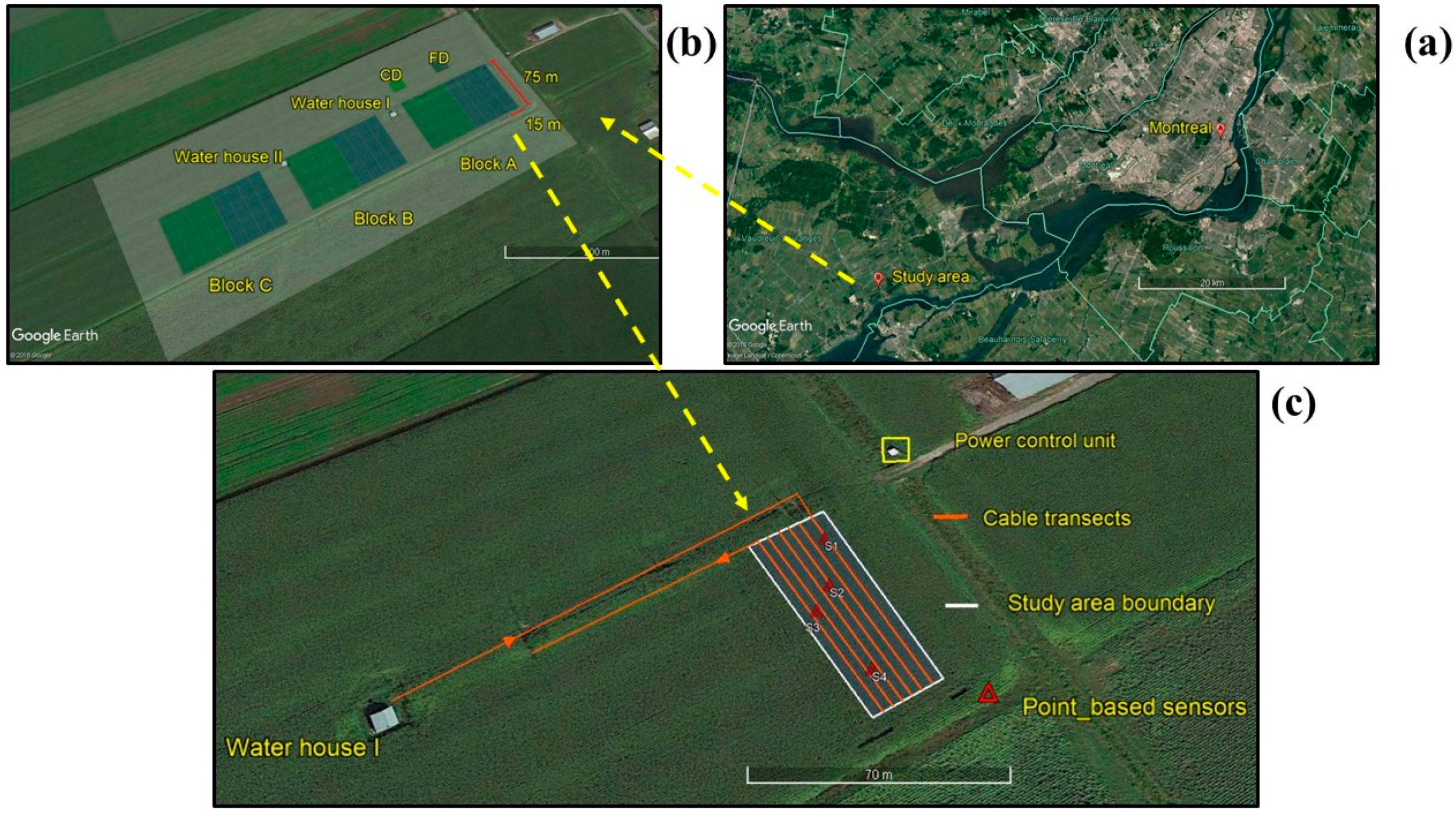
The study site was a 4.2 ha experimental corn field located near Coteau-du-Lac, Québec, Canada (Figure 1a) approximately 60 km west of Montréal. The soil is classified as a Planosol (WRB) (Soulanges very fine sandy loam) [33], has a mean depth of 0.50–0.90 m and overlies clay deposits from the Champlain Sea. The field has a flat topography, with an average slope of less than 0.5% [34]. The study site consisted of three blocks (A, B and C) and each block comprised eight subplots (15 m × 75 m) (Figure 1b). In the center of each subplot, a tile drain had been installed at 1.0 m depth. These drains discharge into two buildings located on the northern side of the field (Figure 1b). Heating and ventilation help to keep a thermally stable environment inside each building which facilitates year-round measurement of drainage volume.
2.2. Soil Water Measurement
Soil water measurements were obtained using two sensor types, namely, a point-based sensor (5TE, Decagon Inc., Pullman, Washington, USA) and a distributed soil water sensor developed using the AHFO technique. The point-based sensor measured SWC every five min while the distributed soil water sensor measured SWC every six hours during the experimental period. The distributed soil water sensor (i.e., AHFO) measured SWC every 0.5 m along six, 64 m long parallel cable transects at the three depths covering 768 locations of the experimental site. The point-based sensors measured SWC at four locations and three depths (i.e., 0.04, 0.12 and 0.20 m) (Figure 1c). Soil water content measured from both sensing techniques were averaged temporally (i.e., to daily scales) and spatially (N = 3 for 5TE and N = 768 for AHFO) for soil water balance calculations. Soil water data from only three 5TE sensor locations were used to calculate the spatially averaged SWC due to a technical problem at one location. ΔSWS was calculated using the volumetric soil water contents (θv, mm3 mm−3) measured at respective depths using
where θv measurements were integrated over each soil layer zi (mm) for a given time interval Δt (days) to obtain ΔSWS. There were three layers: (1) 0–0.08 m, (2) 0.08–0.16 m and (3) 0.16–0.24 m. It was assumed that each soil layer was homogenous and that θv measured in the middle of each layer (i.e., 0.40, 0.12 and 0.20 m) was representative of the layer. Therefore, an integration interval () of 0.08 m was used for each depth and SWS was calculated to a 0.24 m depth from the surface of the soil.
2.3. Development of the Distributed Soil Water Sensor Using Actively Heated Fiber-Optics
The AHFO technique is based on the distributed temperature sensor (DTS), which measures the temperature at high spatial (<1 m) and (1 s) resolutions along a fiber-optic cable, potentially exceeding 10 km in length. More details on the development, calibration, and validation of the AHFO technique can be found in Vidana Gamage et al., [27]. However, a brief summary of the development, calibration, and validation of the AFHO technique is presented here. A DTS (Linear Pro series, AP Sensing, Germany), consisting of two channels with a maximum measurement range of 4 km was used in this study. The AHFO technique applies an electrically generated heat pulse to the metal sheath of the fiber-optic cable and the resulting temperature change (thermal response) during (heating phase) or after (cooling phase) the heat pulse is related to the water content of the soil using either empirically or physically-based equations. 240 volts were applied to each cable section of 147.3 m long (three cable sections per depth) to produce heat pulses of 7.28 W m−1. Heat pulses were sent for five minutes duration at every six hours during a day starting from 12.00 a.m. on the morning of 22 July 2016 to the 6.00 p.m. on the evening of 17 October 2016. The DTS recorded the thermal response (i.e., temperature increase) every 30 s (temporal) and 0.5 m sampling interval (spatial) of the fiber-optic cable during the heating. The integral of the cumulative temperature increase (Tcum) [7] during a heat pulse was calculated at each point of the fiber-optic cable using
where Tcum is the integral of the cumulative temperature increase (°C s) during the total time of integration t0 (s) at a given point of the cable, ΔT is the DTS recorded temperature change from the pre-pulse temperature (°C). In this study, the average temperature calculated over five minutes prior to each heat pulse was used as the pre-pulse temperature. This average was subtracted from the temperature during the pulse to obtain the temperature increase, ΔT. Tcum was then calculated as the sum of the values obtained by multiplying ΔT by the time interval (30 s) between measurements. Tcum was normalized by power intensity (q) of 7.28 W m−1 as Tcum_N using
Tcum_N is a function of soil thermal properties such as the thermal conductivity; higher thermal conductivity (high SWC), will lead to a higher rate at which the heat is conducted away from the cable resulting in a low Tcum_N at a given point on the cable. Depth-specific empirical calibration relationships between the Tcum_N and SWC were developed using the Tcum_N and SWC data collected at reference cable locations. Independent SWC data measured using nine calibrated 5TE soil moisture sensors (Decagon Devices, Pullman, WA, USA) were used to develop the calibration and validation relationships. Root mean square error (RMSE) was calculated to obtain the averaged predictive accuracy. Soil water content at each 0.5 m length of the cable transects was subsequently obtained from the Tcum_N-SWC calibration relationships at respective depths.
2.4. Weather and Drainage Data
Daily total precipitation (P) data measured at a weather station located about 500 m from the experimental site were used for the water balance calculations. Evapotranspiration (ET) was measured on site at 30 min resolution using the EC technique [1]. The EC system consisted of a three-dimensional sonic anemometer (CSAT-3, Campbell Scientific, Edmonton, Canada) and an open-path infrared gas analyzer (IRGA; LI-7500A, LI-COR, Lincoln, NE, USA). All data were recorded at 10 Hz via an analyzer interface unit (LI-7550, LI-COR Biogeosciences, Lincoln, NE, USA). The ET data were summed to obtain the daily ET. Drainage outflows were measured at the outlet of each tile drain in the control buildings, using tipping buckets. Each tipping bucket has a capacity of 1 L and is connected to a DAQ computer that logged cumulative outflows. Each sub-plot had one outlet, and individual daily drainage flows were used from each subplot.
2.5. Soil Water Balance
Water balance in the root zone for a given time period (Δt) is given by
where P and ET are as defined previously, I is the amount of irrigation water applied, R is surface runoff, D is drainage below the root zone, is change in soil water storage measured by distributed or point-based soil water sensors within 0.24 m depth and Re is the residual component. R was assumed to be negligible due to the flat topography of the study area and there was no irrigation during the study period. All components are expressed in units of length (mm).
The residual component reflects the lack of water budget closure and represents the sum of the lateral flows, SWS from the deeper layers (>0.24 m) and measurement errors of the different water balance components. Because the ΔSWS was only estimated for the top 0.24 m depth for both sensor types, while the drainage below the root zone (D) was measured at a greater depth (0.90 m), the ΔSWS from both sensor types will likely be underestimated, resulting in an increased Re. However, since both sensors should suffer from the same lack of depth information, the sensor which minimized Re from
was considered to provide the best field-scale estimation of SWS.
For both point-based (N = 3) and distributed (N = 768) sensors, spatially averaged θv were used to calculate the ΔSWS using Equation (1). The ΔSWS calculated from the point-based and distributed sensing techniques were denoted as ΔSWS_5TE, and ΔSWS_AHFO, respectively. The ΔSWS was also calculated from the simple water balance (using components of the left side of Equation (4)) and denoted as ΔSWS_WB. In all cases, ΔSWS was calculated for the entire measurement period (2.5 months) and subsets ranging from days to weeks (Table 1). The agreement between ΔSWS_WB and ΔSWS_5TE or ΔSWS_AHFO was assessed by the correlation coefficient (r). Furthermore, the difference between ΔSWS calculated from each sensor (i.e., ΔSWS_5TE or ΔSWS_AHFO) and ΔSWS_WB was calculated (using Equation (5)) as Re and is presented in Table 1.
In addition to the comparison of ΔSWS_AHFO and ΔSWS_5TE to ΔSWS_WB, ΔSWS_AHFO and ΔSWS_5TE were used to estimate the evapotranspiration (ET*) using
ET* is the estimated evapotranspiration either using the ΔSWS_AHFO or ΔSWS_5TE and P and D, and is as defined previously. ETε error in ET estimation can be estimated using
The soil water sensing technique that provided the lowest ETε was considered to provide the closest estimate of ET as compared with that measured using EC.
Independent two-sample Wilcoxon test (a non-parametric independent two-sample test) was conducted to test if there was any significant difference between the Re means and between the ETε means estimated from the two sensing techniques at p < 0.05 probability level. The relative reduction in error (RRE) was calculated as the difference between Re for the distributed and point-based sensors (for water balance) and expressed as a percentage of the computed Δ SWS_WB.
3. Results and Discussion
3.1. Calibration and Validation of the Soil Water Sensors
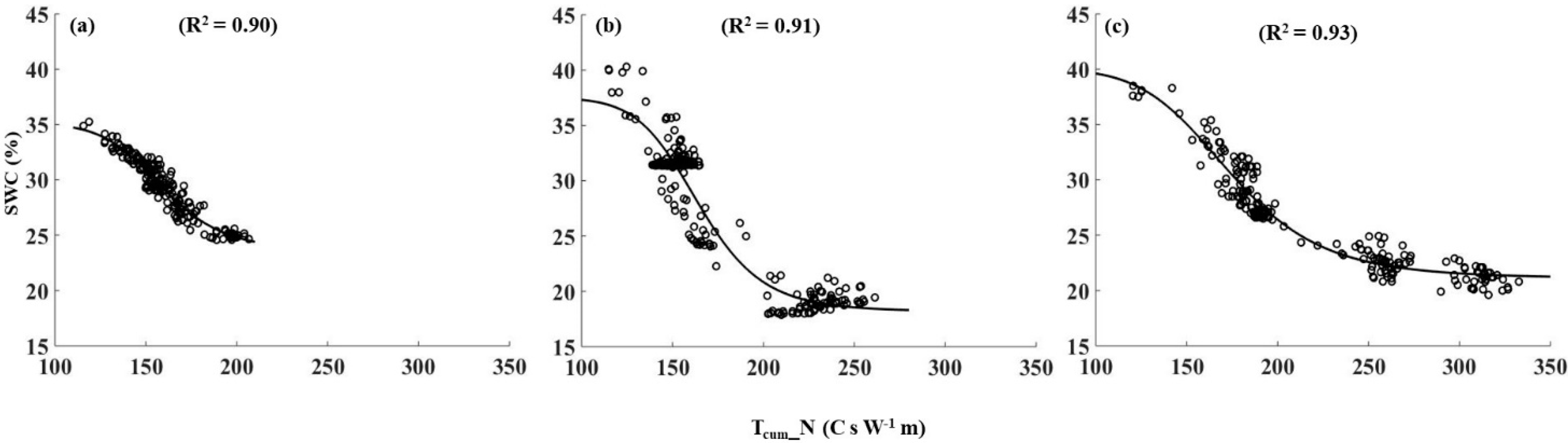
The relationship between Tcum_N and SWC was stronger for all three depths (0.05 m: R2 = 0.90; 0.10 m: R2 = 0.91; 0.20 m: R2 = 0.93), with RMSEs of 0.08, 0.12, and 0.18, respectively (Figure 2). Calibration relationships showed a similar shape for all the depths despite the differences in the maximum and minimum SWC values. The sensitivity of Tcum_N was relatively low in dry soil (<20%), and it started to increase at an increasing rate, with the rate decreased after reaching a SWC between 35% and 40% for all the depths (Figure 2). These results are comparable with the findings by Sayde et al. [21], who observed a lower sensitivity of Tcum_N at higher water contents. However, most of the SWC values measured during the experimental period fell within the range of 15–35%, while only a few values were found between 35 and 40%. Therefore, the distributed soil water sensor could measure the SWC accurately across a wider SWC range. Root mean square error of calibrated point-based sensors was 2%, which suggested a good measurement accuracy. In comparison to the calibrated point-based sensors (gravimetrically), the distributed water sensor showed predictive accuracies of RMSE of 3.3, 2.8 and, 3.7% for 0.04, 0.12 and 0.20 m depths, respectively.
3.2. Comparison of the Distributed Sensor with the Point-Based Sensor
Overall, both point-based and distributed sensors failed to close the water balance, and underestimated the ΔSWS_WB for the selected time periods (Figure 3a), which was primarily due to a lack of SWC measurements from layers >0.24 m. Therefore, we focused the discussion mainly on a comparison of the residual, Re between the two sensors and the magnitude of the RRE%. Because the absolute values of Re estimated from distributed sensor were always lower than those of the point-based sensor, a larger RRE% indicated a better performance of the distributed sensor for estimating the overall ΔSWS. The residual component, Re, represented the sum of the lateral flows, SWS within layers beneath the measurement zone (>0.24 m), and any measurement errors of the different water balance components (i.e., ET, P, D, and soil water content). Estimates of P can have a wide range of error, depending on the gauge placement, gauge spacing, and areal averaging technique [35]. In addition to the errors associated with the gauges, a considerable error can result from the ambient wind speed [36,37]. Though ET was estimated at high temporal resolutions using the EC technique, the footprint of the measurement is not fixed in time [38,39], and this could introduce an additional error. The vertical plastic barriers between the plots were installed in 1992 and extended to 1.5 m into the ground. Some seepage between plots can occur below this point, as the soil at 1.5 m depth is not impermeable. Therefore, some errors associated with estimates of D could also contribute the Re component. However, D, ET and P contribute the same error for the estimations of water balance using each of the soil water sensing techniques. The underestimation of SWS from the lack of deep measurements is also similarly common between the sensors. Therefore, differences resulting between the two Re estimates are due to the water sensing techniques.
The correspondence between the ΔSWS_AHFO and ΔSWS_WB was strong for the ΔSWS flux <60 mm range, but the discrepancy was higher when the ΔSWS flux was >60 mm (Figure 3a). In contrast, the point-based sensor consistently underestimated the ΔSWS_WB and showed a higher discrepancy (Figure 3a). The poor agreements between ΔSWS_AHFO and ΔSWS_WB were attributed to three time periods where ΔSWS_WB was above 60 mm (Figure 3a). Large P events that occurred during these periods likely caused the infiltration front to penetrate beyond 0.24 m depth and this, therefore, was not captured by the either the distributed or point sensor. For example, the highest ΔSWS of 117 mm was reported for the whole experimental period from 22 July to 12 September 2016, and that period included two P events of >20 mm. Therefore, a smaller difference of Re (23 mm) between the two sensors was observed during this period (Table 1). However, the ΔSWS_AHFO showed an excellent agreement with ΔSWS_WB after removing the three periods from the correlation analysis; r between ΔSWS_AHFO and ΔSWS_WB increased to 0.95, while r between ΔSWS_5TE and ΔSWS_WB only increased to 0.70 (Figure 3b). The results clearly showed that the distributed sensor outperformed the point-based sensor when there was a minimal loss of water to deeper layers (>0.24 m).
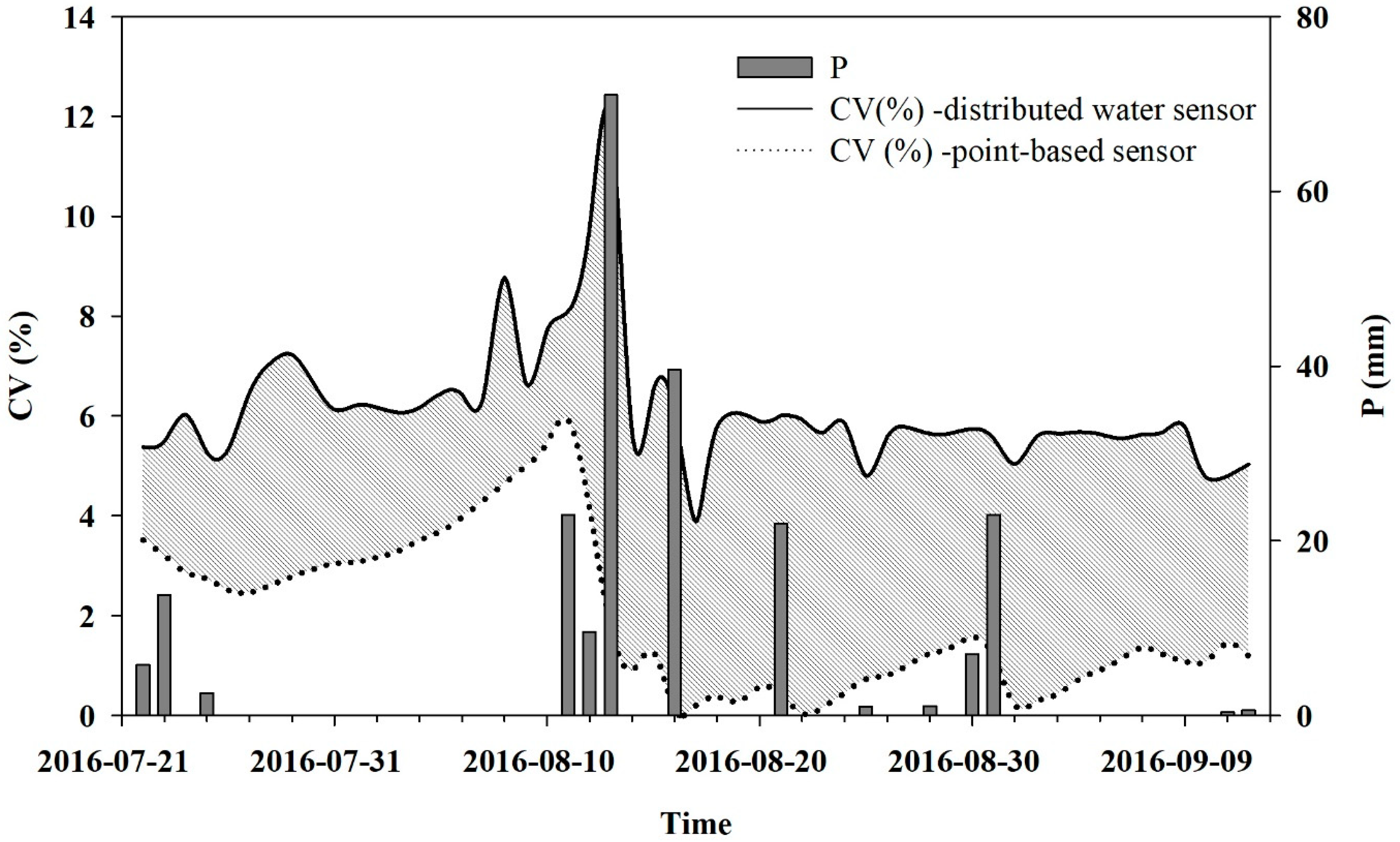
The strength of the agreement between each sensor-measured ΔSWS and ΔSWS_WB during the periods of <60 mm ΔSWS mainly depended on the ability of a particular sensor to capture the spatial variability of SWC and to provide a more accurate estimate of ΔSWS at the field scale. The coefficient of variation (CV) of SWC measured by the distributed sensor was consistently higher than that of the point-based sensors (Figure 4), thus indicating that the distributed sensor captured more spatial variability of SWC than that of the point-based sensors during the whole experimental period. According to Blöschl and Sivapalan [40], the variability of the SWC could be affected by the three types of scales: spacing, support, and extent. Spacing refers to the distance (or time) between the measurements, support to the averaged volume or area (or time) of a single measurement, and extent to the overall coverage of the measurements (in space or time). In this study, the spacing between the point-based sensors was larger (26–46 m) compared to that of the distributed sensor (0.5 m), and apparently, the point-based sensors failed to capture the small-scale variability in the field throughout the experimental period and contributed to the difference between the CVs for distributed and point-based sensors. A larger difference between the CVs for distributed and point-based sensor (shaded area in Figure 4) during the wetter period (after 10 August) indicated that the distributed sensor captured a substantial amount of small-scale variability in wetter periods. Both sensors captured the spatial variability of SWC during the drier period while the distributed sensor likely gave more accurate magnitude during this period (Figure 4).
When the time period considered for water balance calculation was longer, ΔSWS at deeper layers (>0.24 m) caused by either wetting (by P) or drying (by ET) was substantial, and therefore, this resulted in a relatively larger Re. For example, time periods from 22 July to 12 September and 22 July to 4 September showed larger Res for both sensor types (Table 1). ET influenced ΔSWS at deeper (>0.24 m) layers significantly at the beginning and intense P events (>20 mm) also caused a substantial ΔSWS at deeper layers in the middle and end of the periods. When shorter time periods were considered, Res of both sensor types were relatively smaller than that of the longer time periods, but substantial differences between the Re of point-based sensor and that of the distributed sensor were only observed for relatively wet time periods (Table 1). Therefore, the distributed sensor showed a better performance on estimating overall ΔSWS for shorter wet periods. For example, the highest RREs of 62%, 50%, and 42% were reported for the periods of 24 August to 1 September, 23 August to 1 September, and 23 August to 25 August, respectively (Table 1). Despite the shorter time period, the lowest RRE of 8% was reported for the drier period from 22 July to 14 August (Table 1), which indicated that the distributed sensor showed a little improvement in reducing the Re. These results indicated that the distributed sensor outperformed the point-based sensor, by capturing more small-scale spatial variability of soil water content, particularly during the shorter wet periods.
Results of the two-sample Wilcoxon test statistically verified these observations. Results showed no significant difference between the median Re of the point-based sensor and that of the distributed sensor (n = 14 and p = 0.11) when all the time periods were considered. However, the median Re of the point-based sensor was significantly higher than that of the distributed sensor (n = 7 and p = 0.03) when only the shorter wet periods were included (Figure 5).
3.3. Comparison of Evapotranspiration Estimates
Overall, both point-based and distributed sensors underestimated the ET (Table 2), likely due to the lack of SWC measurements from deeper layers which was similarly common between the two sensing techniques. Therefore, any differences in the ETε or cumulative ETs between the two sensing techniques could be attributed to the performance of the two soil water sensing techniques. ETε ranged from 115 mm to 4.6 mm and 113 mm to −2.7 mm for the point-based and distributed sensing techniques, respectively. The two sensing techniques showed no difference in ET* for the period from 22 July to 12 August, and both sensing techniques underestimated ET by 115 and 113 mm, respectively (Table 2). Furthermore, the discrepancy between the cumulative ET of the distributed sensor and that of the point-based sensor was negligible during the early dry period, while cumulative ETs of both sensors showed a least match to the EC measured ET during this period (Figure 6). Both sensors failed to capture the amount of water that was removed from the deeper soil layers (>0.24 m) by the ET during the early dry period from 22 July to 12 August, and this resulted in a larger difference between the cumulative ETs of sensors and cumulative ET measured by EC (Figure 6). There was a smaller difference in the CVs of SWC measured by both sensors during the early dry period (Figure 4), and this likely resulted from a lack of small-scale variability of SWC in dry soil. Therefore, the distributed sensor showed a poor performance in estimating ET during the early dry period.
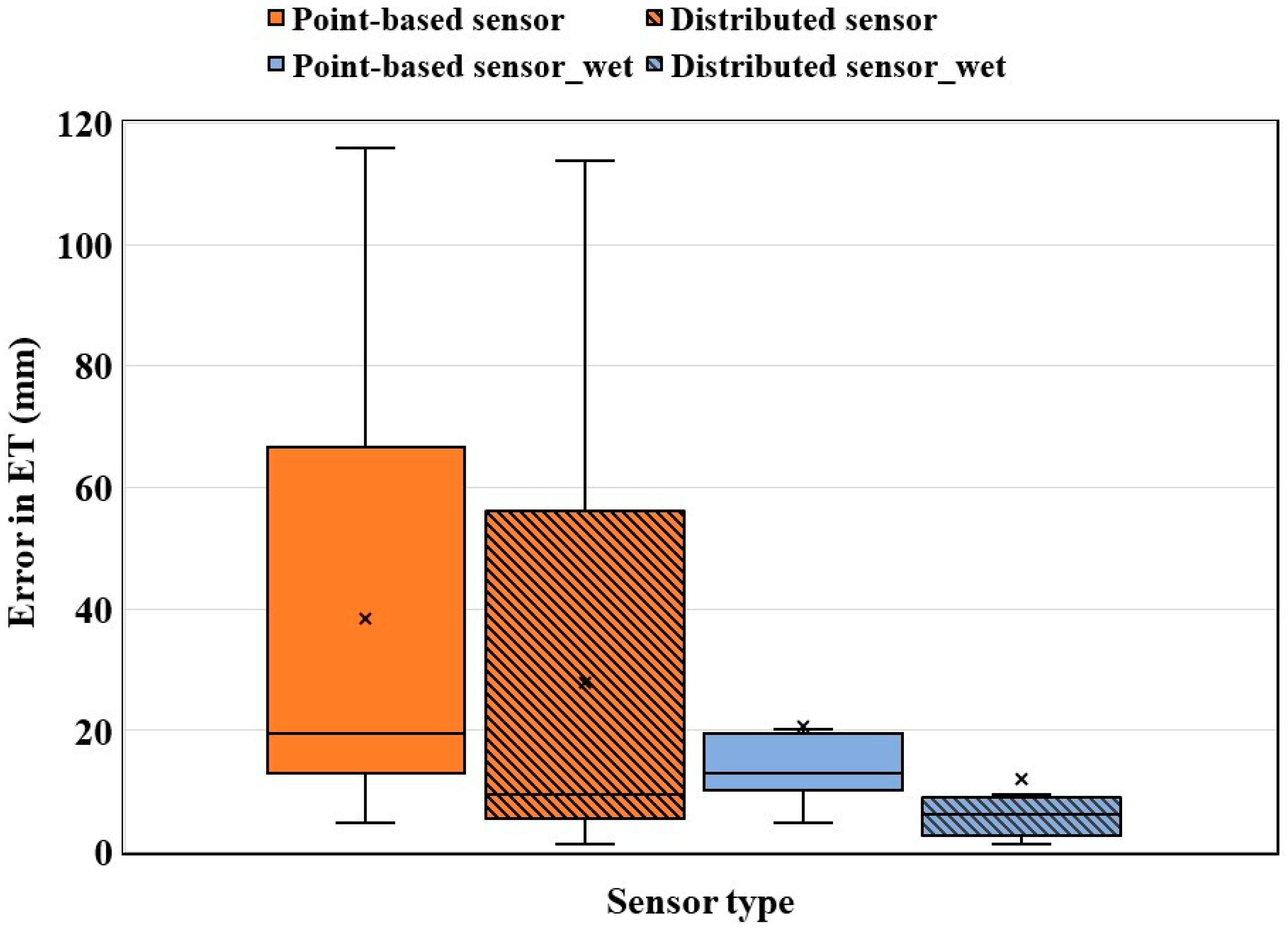
Performance of the distributed sensor in estimating the ET was better and more noticeable for shorter wet periods than the longer periods (Table 2). For example, ETε of distributed sensor decreased by approximately three and four times, respectively, for the periods of 24 August to 01 September and 23 August to 25 August compared to the ETε of the point-based sensor. The cumulative ET of the distributed sensor also exhibited the similar pattern; the cumulative ET of the of the distributed sensor showed a relatively close match to the cumulative ET measured by the EC after 14 August. However, the ETε of the distributed sensor showed no substantial differences to that of the point-based sensor for longer time periods (e.g., from 22 July to 12 September and 22 August to 12 September) (Table 2). The discrepancy between the cumulative ET’s of the two sensors and the cumulative ET measured by EC was also high towards the end of the experimental period (Figure 6). When the time period was longer, ΔSWS at deeper layers, which was brought by P and ET, could be significant, and this might have contributed to larger ETε. These results can be further examined by statistically comparing the medians of ETε of the two sensing techniques including all the time periods as well as including only shorter wet periods. The median ETε of the point-based sensor showed no significant difference from that of the distributed sensor (n = 15 and p = 0.07) when all the time periods were considered. However, the inclusion of only the shorter wet periods resulted in a significant difference between the median ETε of the point-based sensor and that of the distributed sensor (n = 7 and p = 0.01) (Figure 7). Overall, the results from individual time periods and two-sample t-test showed a better performance of the distributed sensor during the shorter wet periods. Soil water content measurements from deeper layers (>0.24 m) are necessary to compare the performance of the two sensors for longer time periods. Because the accuracy of the ET* depended on an accurate average value of ΔSWS obtained from the whole soil profile. Results of ET estimations reinforced the fact that the distributed sensor captured more variability in wetter soils and reduced ETε significantly compared to that of the point-based sensor during the shorter periods.
The distributed soil water sensor (i.e., AHFO) measured SWC at high spatial resolutions (e.g., 0.50 m) and captured more small-scale variability of SWC than that of few point-based sensors. A larger difference between the CVs of the two sensors in wetter periods clearly indicated a dominance of small-scale variability in wet soils, and this was captured by the distributed soil water sensor. The scale of the spatial variability of SWC mainly depends on the scale of the controlling processes. Under wet conditions, the variability is mainly controlled by small-scale variability in hydraulic conductivity and porosity at field scale, while the spatial variability of SWC in dry soils is largely influenced by large-scale processes such ET [41,42,43,44]. However, the scope of this study was only to compare the performance of the two sensors on closing the water balance. Hence, more analysis is needed to identify the controls of the variability and their season dependency.
4. Conclusions
In this study, we compared the performance of a point-based (5TE) and a distributed soil water sensor (AHFO) on closing the field water balance and estimating the ET in a corn production agricultural field of eastern Canada. The ΔSWS determined using each sensor was compared with the ΔSWS calculated from simple water balance at field scale. The ΔSWS determined using the two sensors was also used to estimate the ET and was compared with ET measured using eddy covariance. Results of this study emphasized the need for SWC measurements from deeper layers (>0.24 m) to close the water balance and accurately estimate the ET, particularly for longer time periods. However, significantly lower Re and ETε of the distributed sensor showed that it could capture more small-scale spatial variability of SWC and outperform the point-based sensor in shorter wet periods. Overall, this study showed the potential of the distributed soil water sensor to provide a more accurate overall value of SWS at field scale and to reduce the errors in water balance. The results of this study also highlighted the need to consider the change in the size of the sampling domain through time in soil water balance studies. It is suggested to include the SWC measurements from deeper layers to better evaluate the performance of the distributed sensor, especially for the longer periods of larger change in soil water storage (i.e., >60 mm) in future studies.
Author Contributions
D.N.V.G. and A.B. conceived and designed the experiment; D.V.G. performed the experiment and analyzed the data and wrote the manuscript. A.B. and I.B.S. contributed to scientific advising and provided a substantial input to improve the paper.
Funding
This project was funded by grants to Asim Biswas from FRQNT (Fonds de recherche du Québec—Nature et technologies, 2015-NC-180817) and NSERC (Natural Sciences and Engineering Research Council of Canada, RGPIN-2014-04100).
Acknowledgments
The authors would also like to thank Helene Lalande for her assistance in the laboratory measurements, and Guy Vincent, Maxime Leclerc and Yakun Zang, Kelly Nugent, Scott MacDonald, Tracy Rankin, Mi Lin and Rasika Burghate for assistance in data collection, sensor cable installation and retrieval in the field.
Conflicts of Interest
The authors declare no conflict of interest.
References
- BaldocchI, D.D. Assessing the eddy covariance technique for evaluating carbon dioxide exchange rates of ecosystems: Past, present and future. Glob. Chang. Biol. 2003, 9, 479–492. [Google Scholar] [CrossRef]
- Evett, S.R.; Schwartz, R.C.; Casanova, J.J.; Heng, L.K. Soil water sensing for water balance, et and wue. Agric. Water Manag. 2012, 104, 1–9. [Google Scholar] [CrossRef]
- Singh, S.; Boote, K.J.; Angadi, S.V.; Grover, K.K. Estimating water balance, evapotranspiration and water use efficiency of spring safflower using the cropgro model. Agric. Water Manag. 2017, 185, 137–144. [Google Scholar] [CrossRef]
- Aggarwal, P.; Bhattacharyya, R.; Mishra, A.K.; Das, T.K.; Šimůnek, J.; Pramanik, P.; Sudhishri, S.; Vashisth, A.; Krishnan, P.; Chakraborty, D.; et al. Modelling soil water balance and root water uptake in cotton grown under different soil conservation practices in the indo-gangetic plain. Agric. Ecosyst. Environ. 2017, 240, 287–299. [Google Scholar] [CrossRef]
- Entekhabi, D. Recent advances in land-atmosphere interaction research. Rev. Geophys. 1995, 33, 995–1003. [Google Scholar] [CrossRef]
- Moran, M.S.; Hymer, D.C.; Qi, J.; Sano, E.E. Soil moisture evaluation using multi-temporal synthetic aperture radar (sar) in semiarid rangeland. Agric. For. Meteorol. 2000, 105, 69–80. [Google Scholar] [CrossRef]
- Akbar, R.; Short Gianotti, D.; McColl, K.A.; Haghighi, E.; Salvucci, G.D.; Entekhabi, D. Hydrological storage length scales represented by remote sensing estimates of soil moisture and precipitation. Water Resour. Res. 2018, 54, 1476–1492. [Google Scholar] [CrossRef]
- AghaKouchak, A.; Farahmand, A.; Melton, F.; Teixeira, J.; Anderson, M.; Wardlow, B.D.; Hain, C. Remote sensing of drought: Progress, challenges and opportunities. Rev. Geophys. 2015, 53, 452–480. [Google Scholar] [CrossRef] [Green Version]
- Wagner, W.; Blöschl, G.; Pampaloni, P.; Calvet, J.-C.; Bizzarri, B.; Wigneron, J.-P.; Kerr, Y. Operational readiness of microwave remote sensing of soil moisture for hydrologic applications. Hydrol. Res. 2007, 38, 1–20. [Google Scholar] [CrossRef]
- Zreda, M.; Desilets, D.; Ferré, T.P.A.; Scott, R.L. Measuring soil moisture content non-invasively at intermediate spatial scale using cosmic-ray neutrons. Geophys. Res. Lett. 2008, 35, L21402. [Google Scholar] [CrossRef]
- Ragab, R.; Evans, J.G.; Battilani, A.; Solimando, D. The cosmic-ray soil moisture observation system (cosmos) for estimating the crop water requirement: New approach. Irrig. Drain. 2017, 66, 456–468. [Google Scholar] [CrossRef]
- Zhu, X.; Cao, R.; Shao, M.; Liang, Y. Footprint radius of a cosmic-ray neutron probe for measuring soil-water content and its spatiotemporal variability in an alpine meadow ecosystem. J. Hydrol. 2018, 558, 1–8. [Google Scholar] [CrossRef]
- Moghadas, D.; Jadoon, K.Z.; McCabe, M.F. Spatiotemporal monitoring of soil water content profiles in an irrigated field using probabilistic inversion of time-lapse emi data. Adv. Water Resour. 2017, 110, 238–248. [Google Scholar] [CrossRef]
- Abdu, H.; Robinson, D.A.; Seyfried, M.; Jones, S.B. Geophysical imaging of watershed subsurface patterns and prediction of soil texture and water holding capacity. Water Resour. Res. 2008, 44, W00D18. [Google Scholar] [CrossRef]
- Saito, H.; Kitahara, M. Analysis of changes in soil water content under subsurface drip irrigation using ground penetrating radar. J. Arid Land Stud. 2012, 22, 283–286. [Google Scholar]
- Satriani, A.; Loperte, A.; Soldovieri, F. Integrated geophysical techniques for sustainable management of water resource. A case study of local dry bean versus commercial common bean cultivars. Agric. Water Manag. 2015, 162, 57–66. [Google Scholar] [CrossRef]
- Consoli, S.; Stagno, F.; Vanella, D.; Boaga, J.; Cassiani, G.; Roccuzzo, G. Partial root-zone drying irrigation in orange orchards: Effects on water use and crop production characteristics. Eur. J. Agron. 2017, 82, 190–202. [Google Scholar] [CrossRef]
- Puy, A.; García Avilés, J.M.; Balbo, A.L.; Keller, M.; Riedesel, S.; Blum, D.; Bubenzer, O. Drip irrigation uptake in traditional irrigated fields: The edaphological impact. J. Environ. Manag. 2017, 202, 550–561. [Google Scholar] [CrossRef]
- Larson, K.M.; Small, E.E.; Gutmann, E.D.; Bilich, A.L.; Braun, J.J.; Zavorotny, V.U. Use of gps receivers as a soil moisture network for water cycle studies. Geophys. Res. Lett. 2008, 35, L24405. [Google Scholar] [CrossRef]
- Gil-Rodríguez, M.; Rodríguez-Sinobas, L.; Benítez-Buelga, J.; Sánchez-Calvo, R. Application of active heat pulse method with fiber optic temperature sensing for estimation of wetting bulbs and water distribution in drip emitters. Agric. Water Manag. 2013, 120, 72–78. [Google Scholar] [CrossRef] [Green Version]
- Sayde, C.; Gregory, C.; Gil-Rodriguez, M.; Tufillaro, N.; Tyler, S.; van de Giesen, N.; English, M.; Cuenca, R.; Selker, J.S. Feasibility of soil moisture monitoring with heated fiber optics. Water Resour. Res. 2010, 46, W06201. [Google Scholar] [CrossRef]
- Ciocca, F.; Lunati, I.; Van de Giesen, N.; Parlange, M.B. Heated optical fiber for distributed soil-moisture measurements: A lysimeter experiment. Vadose Zone J. 2012, 11. [Google Scholar] [CrossRef]
- Sayde, C.; Benitez Buelga, J.; Rodriguez-Sinobas, L.; El Khoury, L.; English, M.; van de Giesen, N.; Selker, J.S. Mapping variability of soil water content and flux across 1–1000 m scales using the actively heated fiber optic method. Water Resour. Res. 2014, 50, 7302–7317. [Google Scholar] [CrossRef]
- Striegl, A.M.; Loheide, I.; Steven, P. Heated distributed temperature sensing for field scale soil moisture monitoring. Groundwater 2012, 50, 340–347. [Google Scholar] [CrossRef] [PubMed]
- Vidana Gamage, D.N.; Biswas, A.; Strachan, I.B. Active heat pulse method with fiber optic temperature sensing to monitor three dimensional wetting patterns under drip irrigation. In Canadian Soil Science Society Annual Meeting; Canadian Society of Soil Science Trent University: Peterborough, ON, Canada, 2017; p. 102. [Google Scholar]
- Vidana Gamage, D.N.; Biswas, A.; Strachan, I.B. Actively heated fiber optics method to monitor three-dimensional wetting patterns under drip irrigation. Agric. Water Manag. 2018, 210, 243–251. [Google Scholar] [CrossRef]
- Vidana Gamage, D.; Biswas, A.; Strachan, I.; Adamchuk, V. Soil water measurement using actively heated fiber optics at field scale. Sensors 2018, 18, 1116. [Google Scholar] [CrossRef] [PubMed]
- Laio, F.; Porporato, A.; Ridolfi, L.; Rodriguez-Iturbe, I. Plants in water-controlled ecosystems: Active role in hydrologic processes and response to water stress: Ii. Probabilistic soil moisture dynamics. Adv. Water Resour. 2001, 24, 707–723. [Google Scholar] [CrossRef]
- Vivoni, E.R.; Moreno, H.A.; Mascaro, G.; Rodriguez, J.C.; Watts, C.J.; Garatuza-Payan, J.; Scott, R.L. Observed relation between evapotranspiration and soil moisture in the north american monsoon region. Geophys. Res. Lett. 2008, 35. [Google Scholar] [CrossRef]
- Detto, M.; Montaldo, N.; Albertson, J.D.; Mancini, M.; Katul, G. Soil moisture and vegetation controls on evapotranspiration in a heterogeneous mediterranean ecosystem on Sardinia, Italy. Water Resour. Res. 2006, 42. [Google Scholar] [CrossRef]
- Vivoni, E.R.; Watts, C.J.; Rodríguez, J.C.; Garatuza-Payan, J.; Méndez-Barroso, L.A.; Saiz-Hernández, J.A. Improved land–atmosphere relations through distributed footprint sampling in a subtropical scrubland during the north american monsoon. J. Arid Environ. 2010, 74, 579–584. [Google Scholar] [CrossRef]
- Alfieri, J.G.; Blanken, P.D. How representative is a point? The spatial variability of surface energy fluxes across short distances in a sand-sagebrush ecosystem. J. Arid Environ. 2012, 87, 42–49. [Google Scholar] [CrossRef]
- Lajoie, P.G.; Stobbe, P.C. Soils Study of Soulanges and Vaudreuil Counties in the Province of Quebec; Edmond Cloutier: Ottawa, ON, Canada, 1951; p. 73. [Google Scholar]
- Kaluli, J.W.; Madramootoo, C.A.; Zhou, X.; MacKenzie, A.F.; Smith, D.L. Subirrigation systems to minimize nitrate leaching. J. Irrig. Drain. Eng. 1999, 125, 52–58. [Google Scholar] [CrossRef]
- Winter, T.C. Uncertainties in estimating the water balance of lakes1. J. Am. Water Resour. Assoc. 1981, 17, 82–115. [Google Scholar] [CrossRef]
- Adam, J.C.; Lettenmaier, D.P. Adjustment of global gridded precipitation for systematic bias. J. Geophys. Res. Atmos. 2003, 108. [Google Scholar] [CrossRef] [Green Version]
- Nešpor, V.; Sevruk, B. Estimation of wind-induced error of rainfall gauge measurements using a numerical simulation. J. Atmos. Ocean. Technol. 1999, 16, 450–464. [Google Scholar] [CrossRef]
- Horst, T.; Weil, J. Footprint estimation for scalar flux measurements in the atmospheric surface layer. Bound.-Lay. Meteorol. 1992, 59, 279–296. [Google Scholar] [CrossRef]
- Baldocchi, D.; Finnigan, J.; Wilson, K.; Falge, E. On measuring net ecosystem carbon exchange over tall vegetation on complex terrain. Bound.-Lay. Meteorol. 2000, 96, 257–291. [Google Scholar] [CrossRef]
- Blöschl, G.; Sivapalan, M. Scale issues in hydrological modelling: A review. Hydrol. Process. 1995, 9, 251–290. [Google Scholar] [CrossRef]
- Famiglietti, J.S.; Rudnicki, J.W.; Rodell, M. Variability in surface moisture content along a hillslope transect: Rattlesnake hill, texas. J. Hydrol. 1998, 210, 259–281. [Google Scholar] [CrossRef]
- Pan, F.; Peters-Lidard, C.D. On the relationship between mean and variance of soil moisture fields. J. Am. Water Resour. Assoc. 2008, 44, 235–242. [Google Scholar] [CrossRef]
- Vereecken, H.; Kamai, T.; Harter, T.; Kasteel, R.; Hopmans, J.; Vanderborght, J. Explaining soil moisture variability as a function of mean soil moisture: A stochastic unsaturated flow perspective. Geophys. Res. Lett. 2007, 34. [Google Scholar] [CrossRef] [Green Version]
- Cornelissen, T.; Diekkrüger, B.; Bogena, H.R. Significance of scale and lower boundary condition in the 3d simulation of hydrological processes and soil moisture variability in a forested headwater catchment. J. Hydrol. 2014, 516, 140–153. [Google Scholar] [CrossRef]
Figure 1.
(a) The location of the study area, approximately 60 km west of Montreal, (b) the study area consists of three main blocks A, B and C. Blue and green rectangles within the main blocks are subplots (15 × 75 m) of free drainage (FD) and controlled drainage (CD), respectively. Two water houses facilitate the measurement of drainage volume from each subplot and (c) the fiber-optic cable configuration in the field which shows a cable connected to the DTS instrument starts from water house I and runs through two subplots at three depths (0.04, 0.12 and 0.20 m), red triangles show the locations of the point-based sensors used for calibration, validation, and point-based measurements. The distributed soil water sensor represents only the fiber-optic cable transects installed within the two sub-plots.

Figure 2.
Calibration relationships between soil water content and Tcum_N (a) 0.04 m, (b) 0.12 m, and (c) 0.20 m depths, respectively.
Figure 2.
Calibration relationships between soil water content and Tcum_N (a) 0.04 m, (b) 0.12 m, and (c) 0.20 m depths, respectively.

Figure 3.
(a) The change in soil water storage computed by the simple water balance (ΔSWS_WB) and spatially averaged change in soil water storage measured by the point-based sensors (ΔSWS_5TE), and measured by the AHFO sensor (ΔSWS_AHFO) (N = 12); and (b) as in (a), after removing the three periods with >60 mm ΔSWS.

Figure 4.
Temporal changes of the coefficient of variation (CV) of soil water content measured by the distributed sensor technique and the point-based sensor. The coefficient of variation was calculated using the spatial mean and the spatial standard deviation of measured soil water contents of distributed sensor (N = 768) and point-based sensor (N = 3). Dark grey colored bars show the rainfall distribution (mm, in the right Y-axis) during the time period. The shaded area shows the difference between the two CV’s of soil water content measured by the two sensors.

Figure 5.
Box and whisker plots showing the distribution of the residual of the water balance, Re (mm) for each sensing technique. Orange plots include Re values from all the time periods (N = 14), and light blue plots include only the wetter time periods (N = 7). The horizontal line and the cross within a box indicate the median and mean Re, respectively. Boundaries of the box indicate the 25th and 75th percentile and whiskers indicate the maximum and the minimum values of Re.

Figure 6.
Cumulative ET measured using eddy covariance (solid black line) and cumulative rainfall (black dotted line) during the experimental period. Solid circles (point-based) and open circles (distributed) sensors show the cumulative ET values (from 22 July to selected dates) estimated using the measured ΔSWS (see Equation (4)).

Figure 7.
Box and whisker plots showing the distribution of the ETε (mm) for each sensing technique. Orange colored plots include ETε values from all the time periods (N = 15) and light blue colored plots include only the wetter time periods (N = 7). The horizontal line and the cross within a box indicate the median and mean ETε, respectively. Boundaries of the box indicate the 25th and 75th percentile and whiskers indicate the maximum and the minimum values of ETε.


Table 1.
Components of the water balance for each time period and the residual component and relative reduction in error (RRE %) calculated from the change in SWS from distributed (i.e., AHFO) and from point-based (i.e., 5TE) sensors.
Table 1.
Components of the water balance for each time period and the residual component and relative reduction in error (RRE %) calculated from the change in SWS from distributed (i.e., AHFO) and from point-based (i.e., 5TE) sensors.
| Period (2016) | Observations (mm) | Residual (mm) | RRE (%) | ||||||
|---|---|---|---|---|---|---|---|---|---|
| P | ET | D | ΔSWS | Re = P − ET − D − ΔSWS | |||||
| WB | 5TE | AHFO | 5TE | AHFO | |||||
| 22 July–14 August | 125.8 | 174.6 | 4.3 | −53.1 | −33.7 | −38.4 | −19.4 | −14.7 | 8.8 |
| 22 July–18 August | 165.4 | 197.2 | 4.4 | −36.2 | −18.6 | −29.3 | −17.5 | −6.9 | 29.4 |
| 22 July–25 August | 188.4 | 235.0 | 4.4 | −51.0 | −11.2 | −28.2 | −39.8 | −22.8 | 33.4 |
| 22 July–31 August | 219.5 | 268.4 | 4.4 | −53.3 | −10.6 | −30.2 | −42.7 | −23.1 | 36.8 |
| 22 July–4 September | 219.5 | 292.0 | 4.4 | −76.9 | −10.3 | −20.9 | −66.6 | −56.0 | 13.7 |
| 22 July–12 September | 219.5 | 332.4 | 4.4 | −117.3 | −9.2 | −32.3 | −108.1 | −85.0 | 19.7 |
| 23 August–25 August | 1.0 | 15.2 | 0.0 | −14.2 | −2.7 | −8.7 | −11.5 | −5.5 | 42.2 |
| 1 September–3 September | 0.0 | 17.0 | 0.0 | −17.0 | −3.9 | −10.3 | −13.1 | −6.7 | 37.7 |
| 24 August–1 September | 32.1 | 46.9 | 0.0 | −14.8 | −3.1 | −12.2 | −11.7 | −2.5 | 62.0 |
| 20 August–12 September | 54.1 | 125.3 | 0.0 | −71.2 | −3.7 | −12.1 | −67.5 | −59.1 | 11.7 |
| 9 August–11 August | 23.0 | 26.5 | 0.0 | −3.5 | −1.1 | −2.3 | −2.4 | −1.2 | 34.0 |
| 20 August–31 August | 54.1 | 61.3 | 0.0 | −7.2 | −2.4 | −9.9 | −4.8 | 2.7 | 28.5 |
| 25 August–2 September | 32.1 | 46.4 | 0.0 | −14.3 | −1.5 | −6.8 | −12.8 | −7.6 | 36.5 |
P = precipitation, ET: Evapotranspiration, D: Drainage, WB: water balance calculated from simple water balance and % RRE: percentage relative reduction in Re.
Table 2.
Components of the water balance and evapotranspiration estimated using change in soil water storage measured from distributed and point-based sensors and the respective error in ET estimations for selected time periods.
Table 2.
Components of the water balance and evapotranspiration estimated using change in soil water storage measured from distributed and point-based sensors and the respective error in ET estimations for selected time periods.
| Period (2016) | Observations (mm) | Estimations (mm) | |||||||
|---|---|---|---|---|---|---|---|---|---|
| P | ET | D | ΔSWS | ET* = P − D − ΔSWS | ETε = ET − ET* | ||||
| 5TE | AHFO | 5TE | AHFO | 5TE | AHFO | ||||
| 22 July–12 August | 54.8 | 171.0 | 2.1 | −2.7 | −5.7 | 55.4 | 57.8 | 115.6 | 113.2 |
| 22 July–14 August | 125.8 | 174.6 | 4.3 | −33.7 | −38.4 | 155.2 | 159.9 | 19.4 | 14.7 |
| 22 July–18 August | 165.4 | 197.2 | 4.4 | −18.6 | −29.3 | 179.7 | 190.3 | 17.5 | 6.9 |
| 22 July–25 August | 188.4 | 235.0 | 4.4 | −11.2 | −28.2 | 195.2 | 212.2 | 39.8 | 22.8 |
| 22 July–31 August | 219.5 | 268.4 | 4.4 | −10.6 | −30.2 | 225.7 | 245.3 | 42.7 | 23.1 |
| 22 July–4 September | 219.5 | 292.0 | 4.4 | −10.3 | −20.9 | 225.4 | 236.0 | 66.6 | 56.0 |
| 22 July–12 September | 219.5 | 332.4 | 4.4 | −9.2 | −32.3 | 224.3 | 247.4 | 108.1 | 85.0 |
| 9 August–11 August | 23.0 | 26.5 | 0.0 | 1.1 | −2.3 | 21.9 | 25.3 | 4.6 | 1.2 |
| 23 August–25 August | 1.0 | 15.2 | 0.0 | 2.7 | −8.7 | −1.7 | 9.7 | 16.9 | 5.5 |
| 24 August–1 September | 32.1 | 46.9 | 0.0 | −3.1 | −12.2 | 35.2 | 44.3 | 11.7 | 2.5 |
| 20 August–12 September | 54.1 | 125.3 | 0.0 | 3.7 | −12.1 | 50.4 | 66.2 | 74.9 | 59.1 |
| 20 August–31 August | 54.1 | 61.3 | 0.0 | 2.4 | −9.9 | 51.7 | 64.0 | 9.6 | −2.7 |
| 25 August–2 September | 32.1 | 46.4 | 0.0 | −1.5 | −6.8 | 33.6 | 38.9 | 12.8 | 7.6 |
| 1 September–3 September | 0.0 | 17.0 | 0.0 | −3.9 | −10.3 | 3.9 | 10.3 | 13.1 | 6.7 |
P = precipitation, ET: evapotranspiration measured by EC, D: drainage, WB: water balance, ET*: evapotranspiration estimated, ETε: error in ET*.
© 2019 by the authors. Licensee MDPI, Basel, Switzerland. This article is an open access article distributed under the terms and conditions of the Creative Commons Attribution (CC BY) license (http://creativecommons.org/licenses/by/4.0/).
Share and Cite
MDPI and ACS Style
Vidana Gamage, D.N.; Biswas, A.; Strachan, I.B. Field Water Balance Closure with Actively Heated Fiber-Optics and Point-Based Soil Water Sensors. Water 2019, 11, 135. https://doi.org/10.3390/w11010135
AMA Style
Vidana Gamage DN, Biswas A, Strachan IB. Field Water Balance Closure with Actively Heated Fiber-Optics and Point-Based Soil Water Sensors. Water. 2019; 11(1):135. https://doi.org/10.3390/w11010135
Chicago/Turabian StyleVidana Gamage, Duminda N., Asim Biswas, and Ian B. Strachan. 2019. "Field Water Balance Closure with Actively Heated Fiber-Optics and Point-Based Soil Water Sensors" Water 11, no. 1: 135. https://doi.org/10.3390/w11010135
Note that from the first issue of 2016, this journal uses article numbers instead of page numbers. See further details here.