Assessing the Potential Impact of Rising Production of Industrial Wood Pellets on Streamflow in the Presence of Projected Changes in Land Use and Climate: A Case Study from the Oconee River Basin in Georgia, United States

Abstract
:1. Introduction
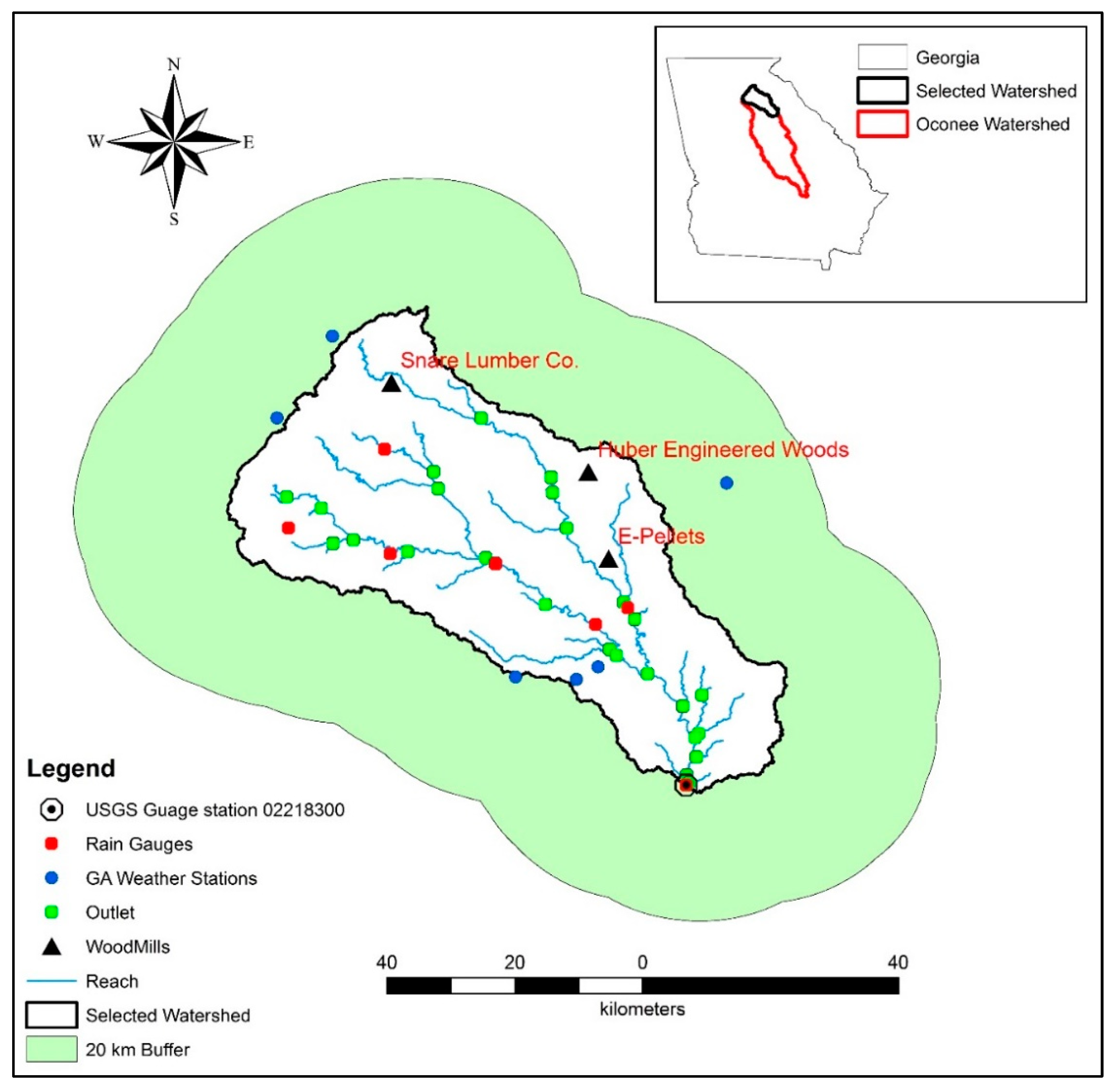
2. Study Area
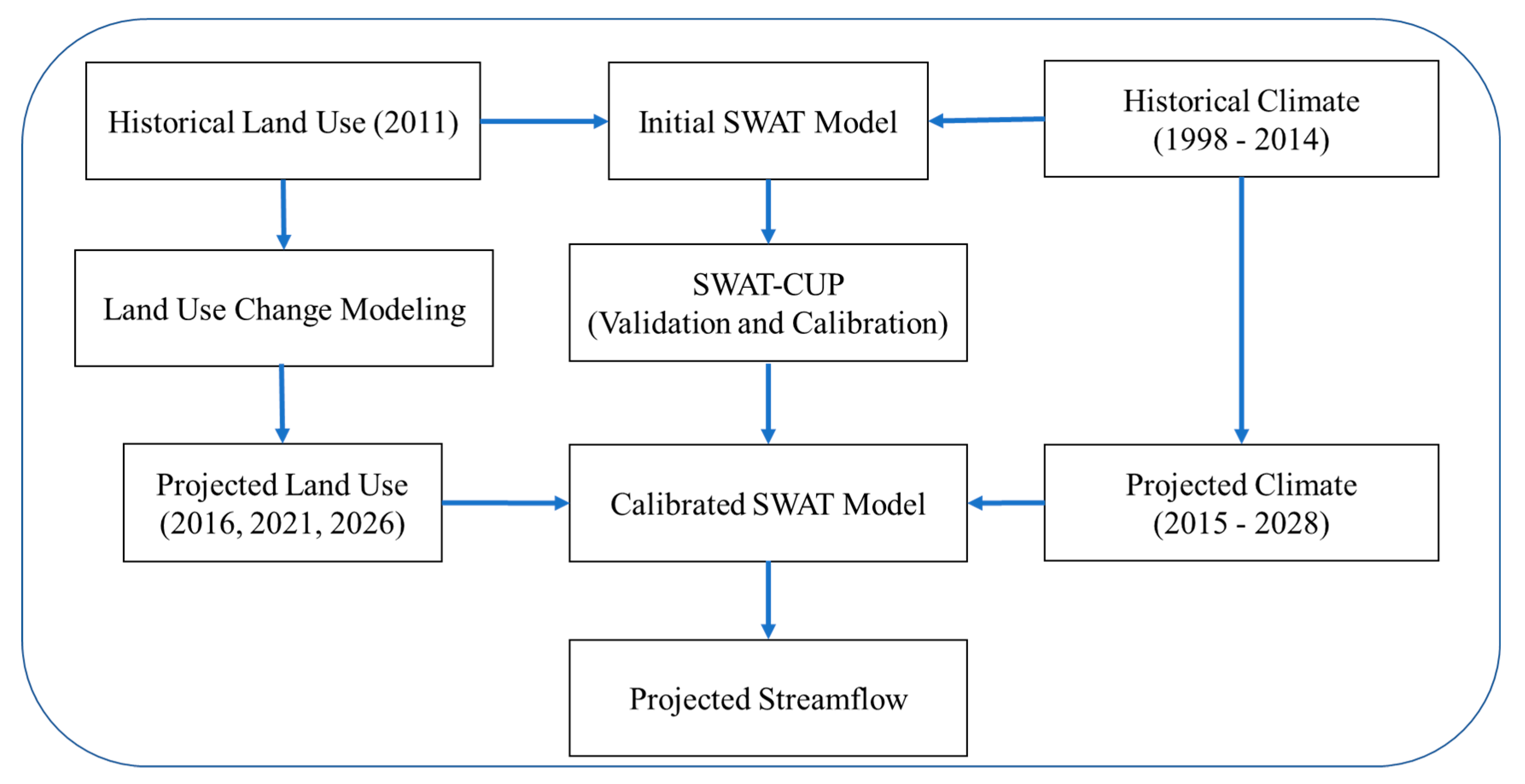
3. Method
3.1. Parameterization, Calibration, and Validation of SWAT
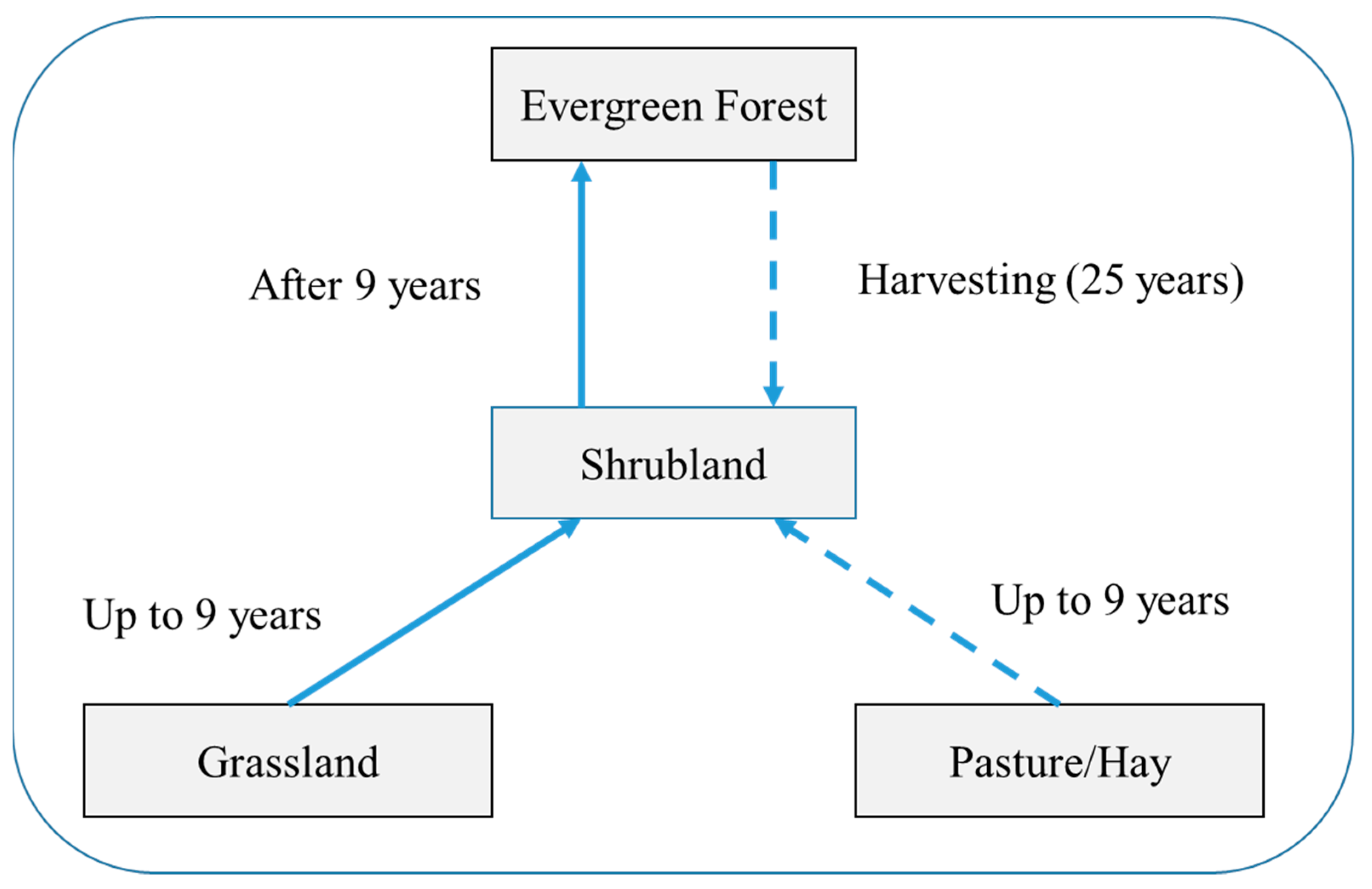
3.2. Land Use Change Modeling
3.3. Ascertaining Changes in Climate
4. Results
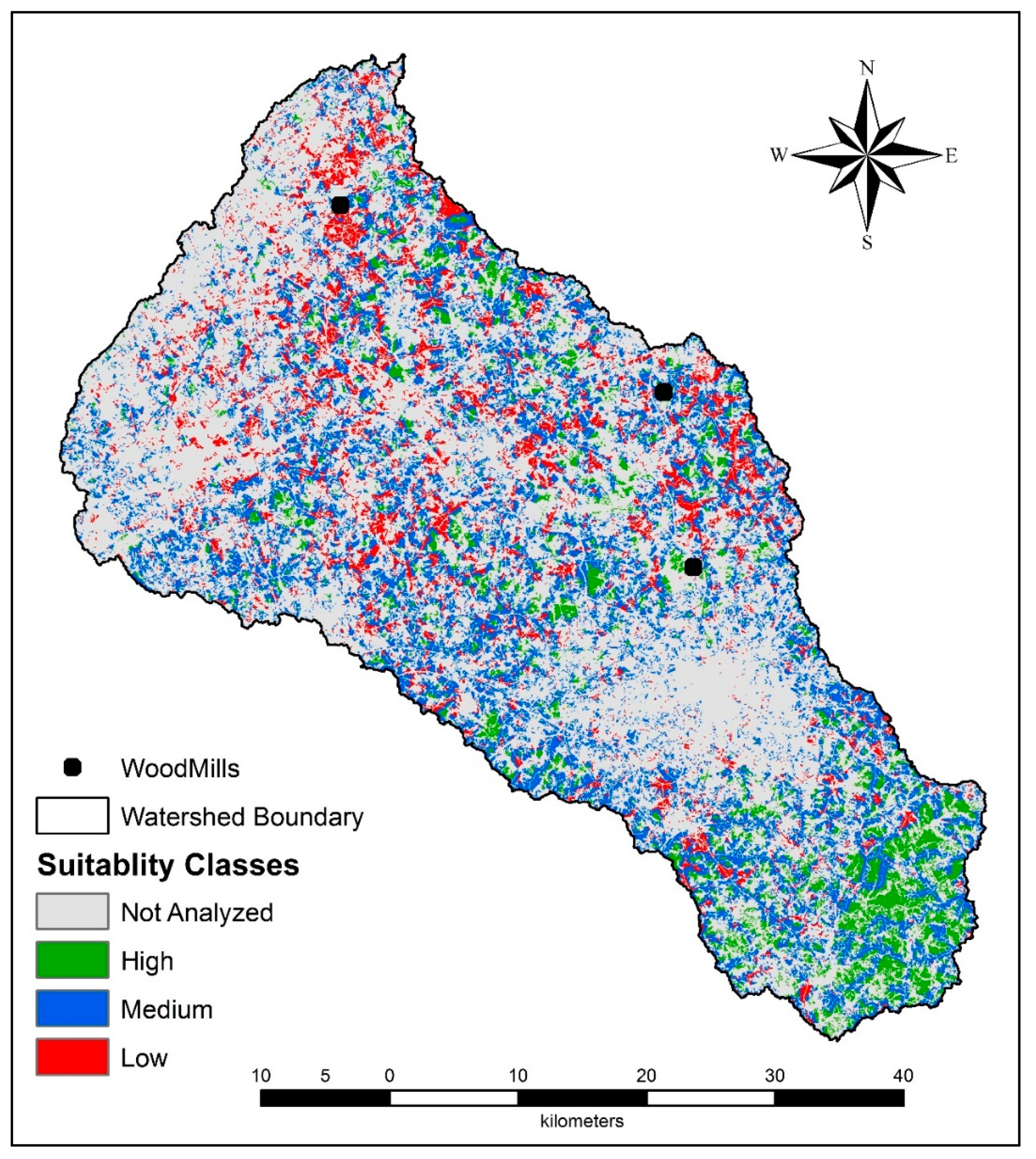
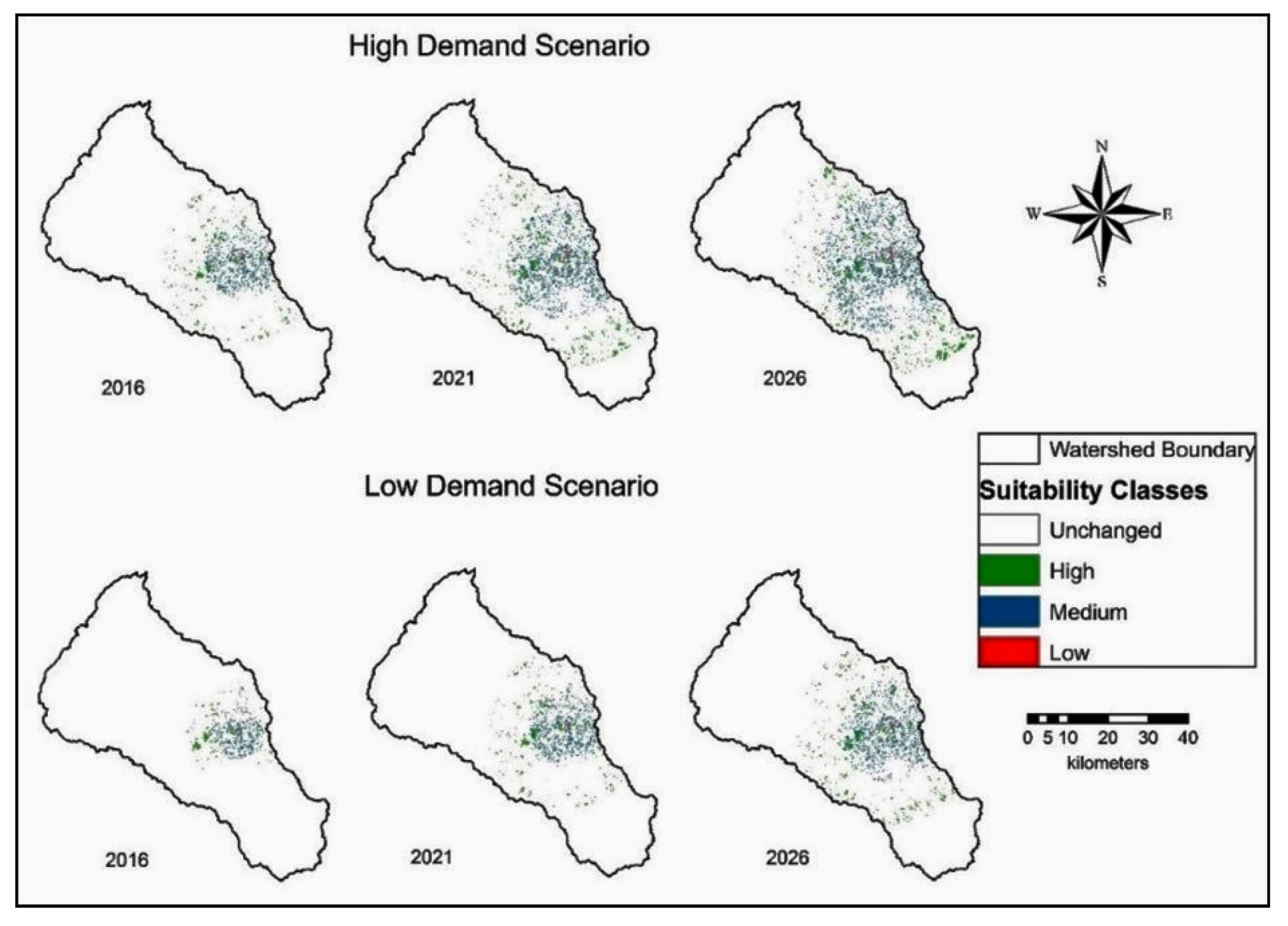
4.1. Suitability Analysis
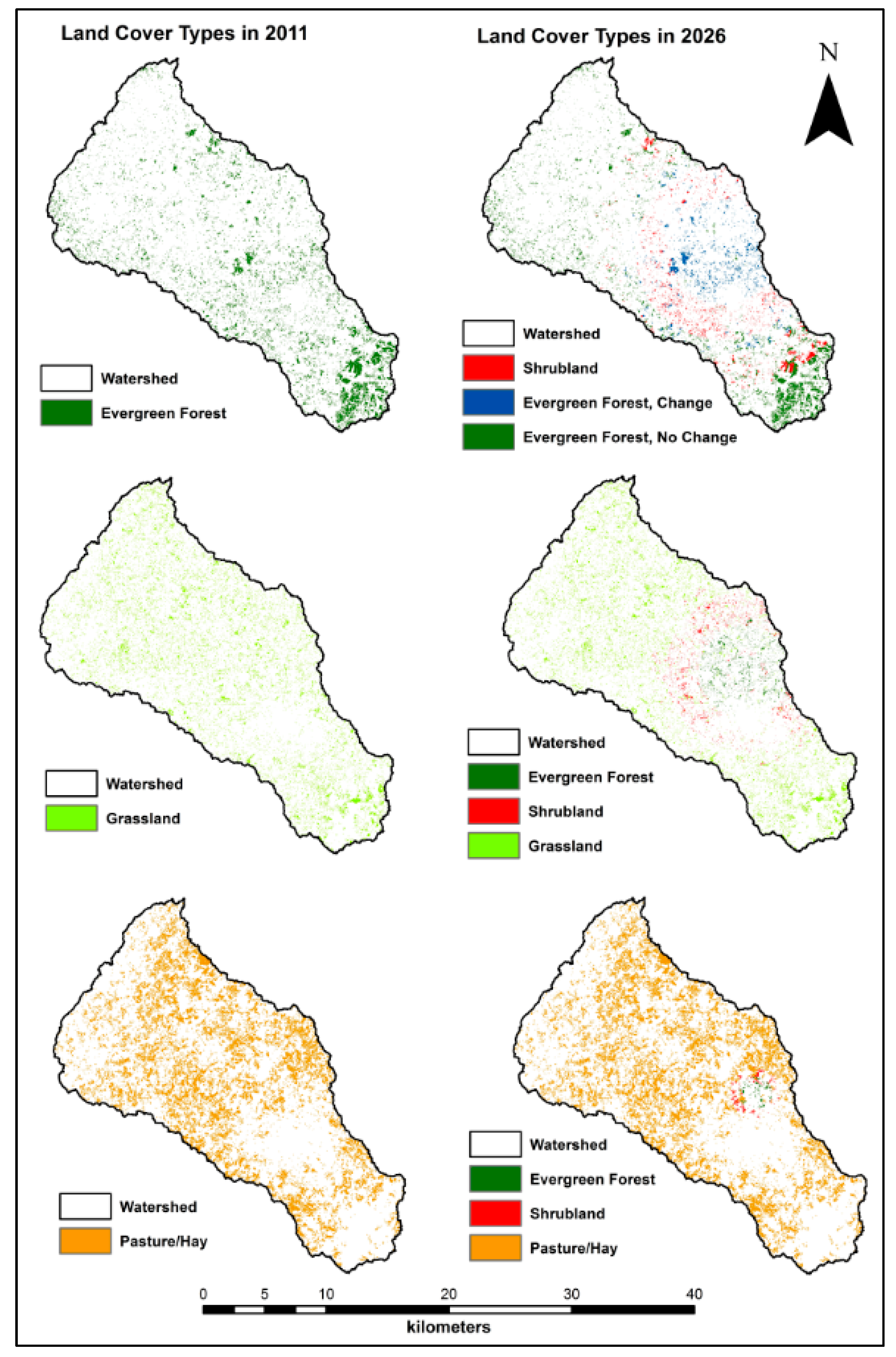
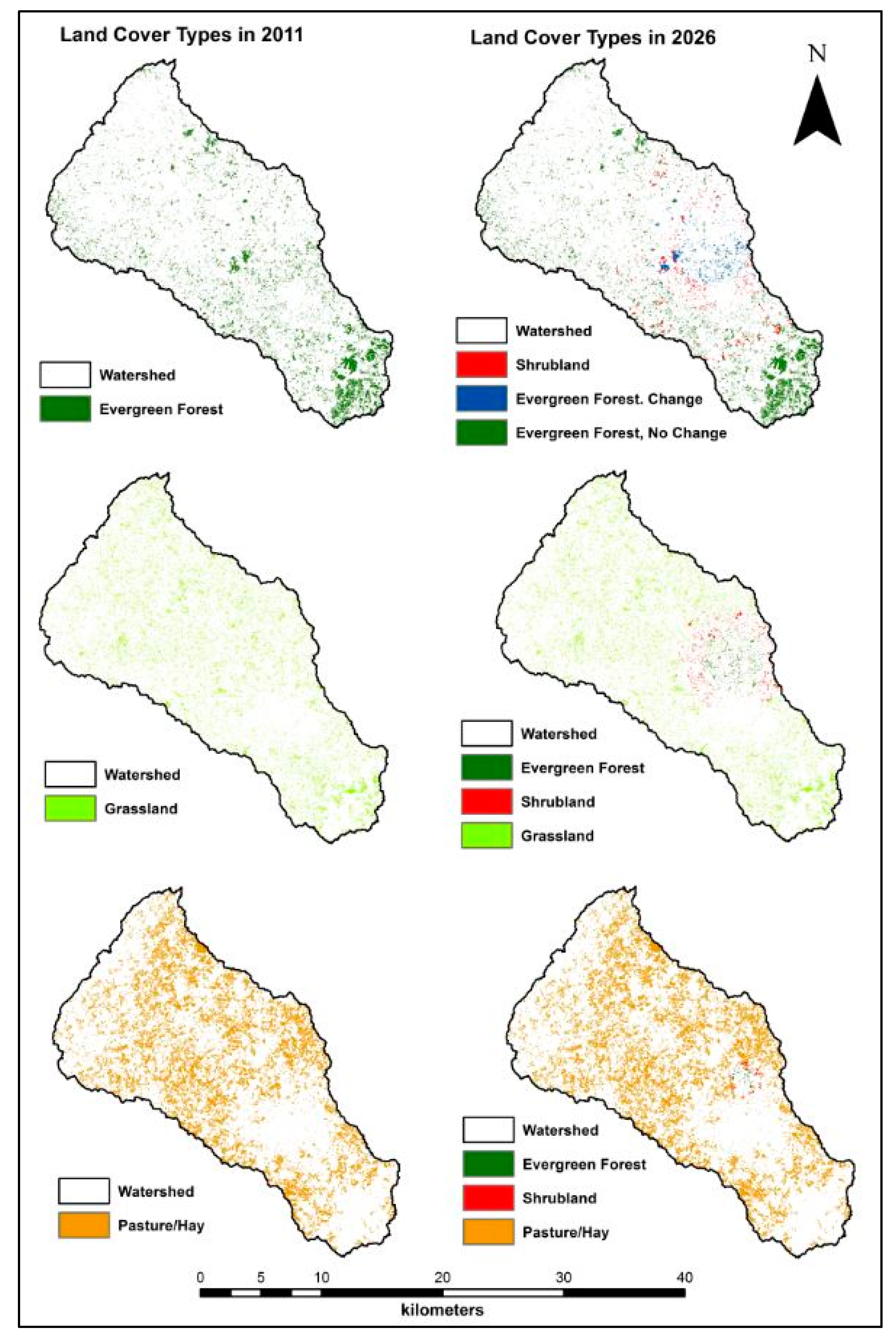
4.2. Land Use Change
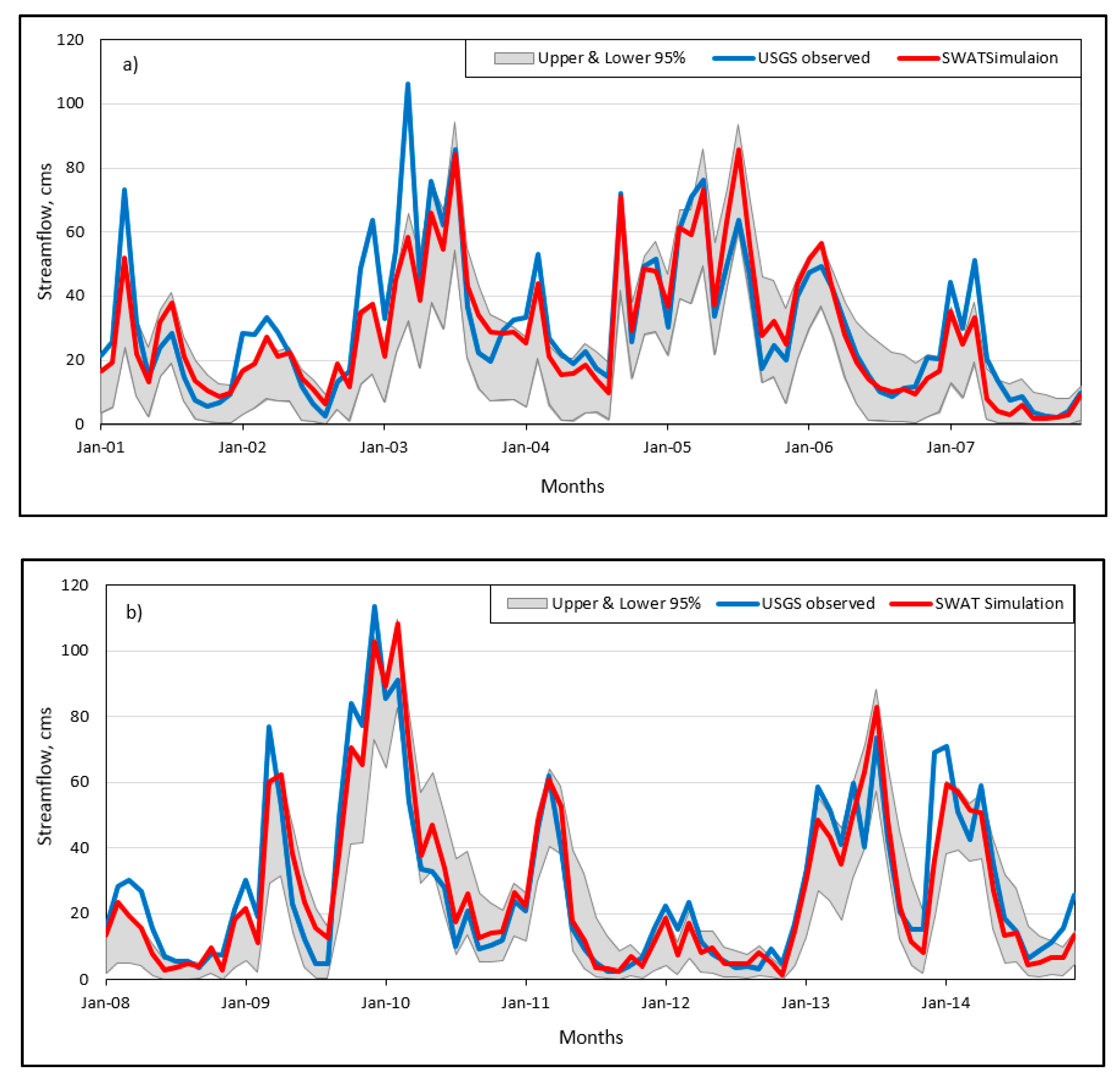
4.3. SWAT Calibration and Validation
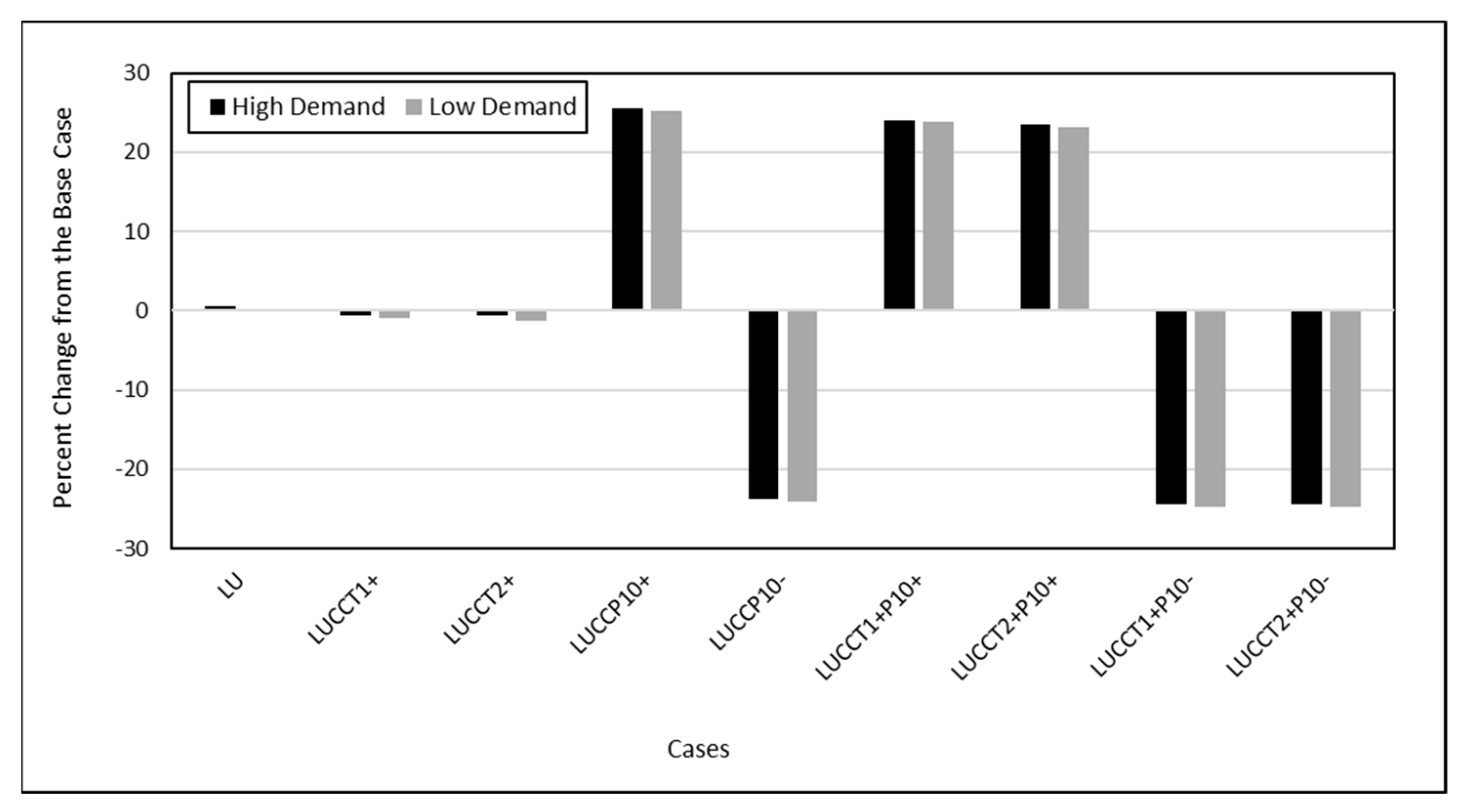
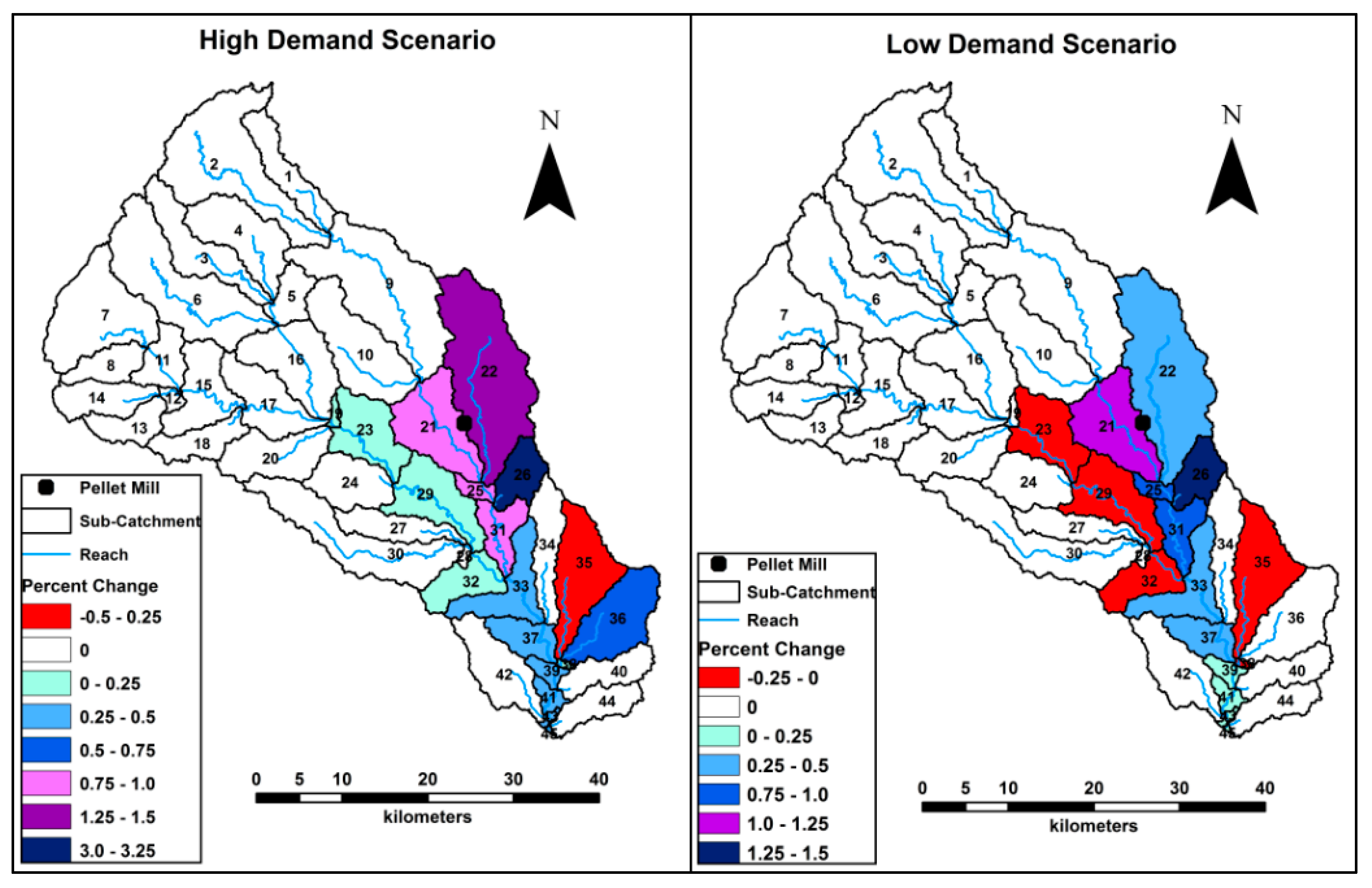
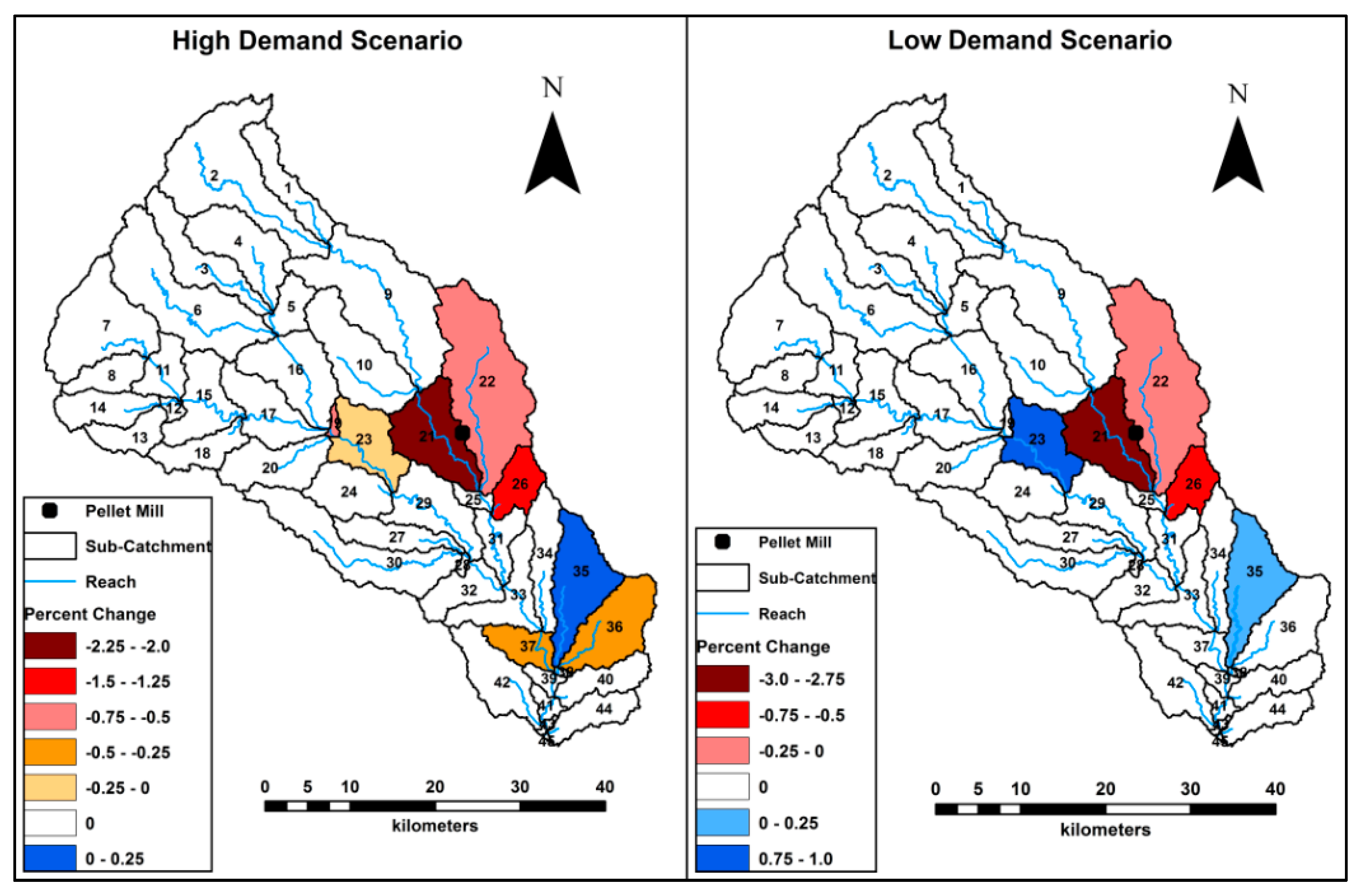
4.4. Land Use and Climate Change Impact on Streamflow
5. Discussion
6. Conclusions
Author Contributions
Funding
Acknowledgments
Conflicts of Interest
References
- Forisk. Wood Bioenergy Update and North American Pellet Capacity: Q3 2016. Available online: http://forisk.com/blog/2016/08/17/wood-bioenergy-update-north-american-pellet-capacity-q3-2016/ (accessed on 20 September 2017).
- European Commission. 2020 Climate & Energy Package. Available online: http://ec.europa.eu/clima/policies/strategies/2020/index_en.htm (accessed on 10 March 2017).
- Wong, P.; Bredehoeft, G.U.S. Wood Pellet Exports Double in 2013 in Response to Growing European Demand. 2014. Available online: http://www.eia.gov/todayinenergy/detail.cfm?id=16391 (accessed on 11 March 2017 ).
- Oswalt, S.N.; Patrick, D.M.; Pugh, S.A.; Smith, W.B. Forest Resources of the United States: A Technical Document Supporting the Forest Service 2020 update of the RPA Assessment; USDA: Washington, DC, USA, 2018. [CrossRef]
- Wang, W.; Dwivedi, P.; Abt, R.; Khanna, M. Carbon savings with transatlantic trade in pellets: Accounting for market-driven effects. Environ. Res. Lett. 2015, 10, 114019. [Google Scholar] [CrossRef]
- Trimble, S.W.; Weirich, F.H.; Hoag, B.L. Reforestation and the reduction of water yield on the southern piedmont since CIRCA 1940. Water Resour. Res. 1987, 23, 425–437. [Google Scholar] [CrossRef]
- Cruise, J.F.; Laymon, C.A.; Al-Hamdan, O.Z. Impact of 20 years of land-cover change on the hydrology of streams in the Southeastern United States. J. Am. Water Resour. Assoc. 2010, 46, 1159–1170. [Google Scholar] [CrossRef]
- Isik, S.; Kalin, L.; Schoonover, J.E.; Srivastava, P.; Lockaby, B.G. Modeling effects of changing land use/cover on daily streamflow: An Artificial Neural Network and curve number based hybrid approach. J. Hydrol. 2013, 485, 103–112. [Google Scholar] [CrossRef]
- Grace, J.M. Forest operations and water quality in the South. Trans. ASAE 2005, 48, 871–880. [Google Scholar] [CrossRef]
- Choi, W.; Deal, B.M. Assessing hydrological impact of potential land use change through hydrological and land use change modeling for the Kishwaukee River basin (USA). J. Environ. Manag. 2008, 88, 1119–1130. [Google Scholar] [CrossRef] [PubMed]
- Zhang, X.N.; Liu, Y.Y.; Fang, Y.H.; Liu, B.J.; Xia, D.Z. Modeling and assessing hydrologic processes for historical and potential land-cover change in the Duoyingping watershed, southwest China. Phys. Chem. Earth 2012, 53–54, 19–29. [Google Scholar] [CrossRef]
- Wijesekara, G.N.; Gupta, A.; Valeo, C.; Hasbani, J.G.; Qiao, Y.; Delaney, P.; Marceau, D.J. Assessing the impact of future land-use changes on hydrological processes in the Elbow River watershed in southern Alberta, Canada. J. Hydrol. 2012, 412–413, 220–232. [Google Scholar] [CrossRef]
- Giri, S.; Arbab, N.N.; Lathrop, R.G. Water security assessment of current and future scenarios through an integrated modeling framework in the Neshanic River Watershed. J. Hydrol. 2018, 563, 1025–1041. [Google Scholar] [CrossRef]
- LaFontaine, J.H.; Hay, L.E.; Viger, R.J.; Regan, R.S.; Markstrom, S.L. Effects of climate and land cover on hydrology in the Southeastern US: Potential impacts on watershed planning. J. Am. Water Resour. Assoc. 2015, 51, 1235–1261. [Google Scholar] [CrossRef]
- Pervez, M.S.; Henebry, G.M. Assessing the impacts of climate and land use and land cover change on the freshwater availability in the Brahmaputra River basin. J. Hydrol. Reg. Stud. 2015, 3, 285–311. [Google Scholar] [CrossRef] [Green Version]
- Wagner, P.D.; Bhallamudi, S.M.; Narasimhan, B.; Kantakumar, L.N.; Sudheer, K.P.; Kumar, S.; Schneider, K.; Fiener, P. Dynamic integration of land use changes in a hydrologic assessment of a rapidly developing Indian catchment. Sci. Total Environ. 2016, 539, 153–164. [Google Scholar] [CrossRef] [PubMed]
- Dwivedi, P.; Khanna, M.; Bailis, R.; Ghilardi, A. Potential greenhouse gas benefits of transatlantic wood pellet trade. Environ. Res. Lett. 2014, 9, 24007. [Google Scholar] [CrossRef] [Green Version]
- Khanna, M.; Dwivedi, P.; Abt, R. Is forest bioenergy carbon neutral or worse than coal? Implications of carbon accounting methods. Int. Rev. Environ. Resour. Econ. 2017, 10, 299–346. [Google Scholar] [CrossRef]
- Fletcher, R.J.; Robertson, B.A.; Evans, J.; Doran, P.J.; Alavalapati, J.R.R.; Schemske, D.W. Biodiversity conservation in the era of biofuels: Risks and opportunities. Front. Ecol. Environ. 2011, 9, 161–168. [Google Scholar] [CrossRef]
- Gottlieb, I.G.W.; Fletcher, R.J.; Nuñez-Regueiro, M.M.; Ober, H.; Smith, L.; Brosi, B.J. Alternative biomass strategies for bioenergy: Implications for bird communities across the southeastern United States. GCB Bioenergy 2017, 9, 1606–1617. [Google Scholar] [CrossRef]
- Zhong, J.; Yu, T.E.; Clark, C.D.; English, B.C.; Larson, J.A.; Cheng, C.L. Effect of land use change for bioenergy production on feedstock cost and water quality. Appl. Energy 2018, 210, 580–590. [Google Scholar] [CrossRef]
- Keerthi, S.; Miller, S.A. Regional differences in impacts to water quality from the bioenergy mandate. Biomass Bioenergy 2017, 106, 115–126. [Google Scholar] [CrossRef]
- Griffiths, N.A.; Jackson, C.R.; Bitew, M.M.; Fortner, A.M.; Fouts, K.L.; McCracken, K.; Phillips, J.R. Water quality effects of short-rotation pine management for bioenergy feedstocks in the southeastern United States. For. Ecol. Manag. 2017, 400, 181–198. [Google Scholar] [CrossRef]
- Christopher, S.F.; Schoenholtz, S.H.; Nettles, J.E. Water quantity implications of regional-scale switchgrass production in the southeastern US. Biomass Bioenergy 2015, 83, 50–59. [Google Scholar] [CrossRef]
- USDA/NRCS Geospatial Data Gateway. Geospatial Data Gateway. United States Department of Agriculture Natural Resources Conservation Service. Available online: https://gdg.sc.egov.usda.gov/ (accessed on 20 March 2017).
- Arnold, J.G.; Srinivasan, R.; Muttiah, R.S.; Williams, J.R. Large area hydrologic modeling and assessment part I: Model development. J. Am. Water Resour. Assoc. 1998, 34, 73–89. [Google Scholar] [CrossRef]
- Neitsch, S.L.; Arnold, J.G.; Kiniry, J.R.; Williams, J.R. Soil and Water Assessment Tool Theoretical Documentation Version 2009; Texas Water Resources InstituteTechnical Report No. 406; Texas A&M University System: College Station, TX, USA, 2011. [Google Scholar]
- Arnold, J.G.; Allen, P.M.; Bernhardt, G. A comprehensive surface-groundwater flow model. J. Hydrol. 1993, 142, 47–69. [Google Scholar] [CrossRef]
- Bingner, R.L. Runoff simulated from Goodwin Creek Watershed using SWAT. Trans. ASAE 1996, 39, 85–90. [Google Scholar] [CrossRef]
- Eckhardt, K.; Ulbrich, U. Potential impacts of climate change on groundwater recharge and streamflow in a central European low mountain range. J. Hydrol. 2003, 284, 244–252. [Google Scholar] [CrossRef]
- Van Liew, M.W.; Arnold, J.G.; Garbrecht, J.D. Hydrologic simulation on agricultural watersheds: Choosing between two models. Trans. ASAE 2003, 46, 1539–1551. [Google Scholar] [CrossRef]
- Wang, S.; Kang, S.; Zhang, L.; Li, F. Modelling hydrological response to different land-use and climate change scenarios in the Zamu River basin of northwest China. Hydrol. Process. 2008, 22, 2502–2510. [Google Scholar] [CrossRef]
- Ozturk, M.; Copty, N.K.; Saysel, A.K. Modeling the impact of land use change on the hydrology of a rural watershed. J. Hydrol. 2013, 497, 97–109. [Google Scholar] [CrossRef]
- Ghaffari, G.; Keesstra, S.; Ghodousi, J.; Ahmadi, H. SWAT-simulated hydrological impact of land-use change in the Zanjanrood Basin, Northwest Iran. Hydrol. Process. 2010, 24, 892–903. [Google Scholar] [CrossRef]
- Fohrer, N.; Haverkamp, S.; Frede, H.G. Assessment of the effects of land use patterns on hydrologic landscape functions: Development of sustainable land use concepts for low mountain range areas. Hydrol. Process. 2005, 19, 659–672. [Google Scholar] [CrossRef]
- Baker, T.J.; Miller, S.N. Using the Soil and Water Assessment Tool (SWAT) to assess land use impact on water resources in an East African watershed. J. Hydrol. 2013, 486, 100–111. [Google Scholar] [CrossRef]
- Lin, Z.L.; Radcliffe, D.E. Automatic calibration and predictive uncertainty analysis of a semidistributed watershed model. Vadose Zone J. 2006, 5, 248–260. [Google Scholar] [CrossRef]
- Neitsch, S.L.; Arnold, J.G.; Kiniry, J.R.; Williams, J.R.; King, K.W. SWAT Manual; USDA, Agricultural Research Service and Blackland Research Center, Texas A&M University: College Station, TX, USA, 2002.
- Soil Conservation Service. Section 4: Hydrology. In National Engineering Handbook; SCS: Washington, DC, USA, 1972. [Google Scholar]
- Hargreaves, G.L.; Hargreaves, G.H.; Riley, J.P. Agricultural benefits for Senegal River Basin. J. Irrig. Drain. Eng. 1985, 111, 113–124. [Google Scholar] [CrossRef]
- Ritchie, J.T. Model for predicting evaporation from a row crop with incomplete cover. Water Resour. Res. 1972, 8, 1204–1213. [Google Scholar] [CrossRef]
- Texas A&M University and USDA–ARS. SWAT: Soil and Water Assessment Tool; Texas A&M University: College Station, TX, USA, 2015.
- Van Liew, M.W.; Veith, T.L.; Bosch, D.D.; Arnold, J.G. Suitability of SWAT for the conservation effects assessment project: Comparison on USDA Agricultural Research Service watersheds. J. Hydrol. Eng. 2007, 12, 173–189. [Google Scholar] [CrossRef]
- Cibin, R.; Sudheer, K.P.; Chaubey, I. Sensitivity and identifiability of stream flow generation parameters of the SWAT model. Hydrol. Process. 2010, 24, 1133–1148. [Google Scholar] [CrossRef]
- Arnold, J.G.; Moriasi, D.N.; Gassman, P.W.; Abbaspour, K.C.; White, M.J.; Srinivasan, R.; Santhi, C.; Harmel, R.D.; van Griensven, A.; Van Liew, M.W.; et al. SWAT: Model use, calibration, and validation. Trans. ASABE 2012, 55, 1491–1508. [Google Scholar] [CrossRef]
- Oliver, C.W.; Radcliffe, D.E.; Risse, L.M.; Habteselassie, M.; Mukundan, R.; Jeong, J.; Hoghooghi, N. Quantifying the contribution of on-site wastewater treatment systems to stream discharge using the SWAT model. J. Environ. Qual. 2014, 43, 539–548. [Google Scholar] [CrossRef]
- Abbaspour, K.C. Swat-Cup 2012: SWAT Calibration and Uncertainty Programs—A User Manual; Eawag, Swiss Federal Institute of Aquatic Sciences and Technology: Dubendorf, Switzerland, 2014. [Google Scholar]
- Shrestha, S.; Dwivedi, P. Projecting land use changes by integrating site suitability analysis with historic land use change dynamics in the context of increasing demand for wood pellets in the Southern United States. Forests 2017, 8. [Google Scholar] [CrossRef]
- Moriasi, D.N.; Gitau, M.W.; Pai, N.; Daggupati, P. Hydrologic and water quality models: Performance measures and evaluation criteria. Trans. ASABE 2015, 58, 1763–1785. [Google Scholar]
- Liu, X.; Sun, G.; Mitra, B.; Noormets, A.; Gavazzi, M.J.; Domec, J.C.; Hallema, D.W.; Li, J.; Fang, Y.; King, J.S.; et al. Drought and thinning have limited impacts on evapotranspiration in a managed pine plantation on the southeastern United States coastal plain. Agric. For. Meteorol. 2018, 262, 14–23. [Google Scholar] [CrossRef]
- Domec, J.C.; Sun, G.; Noormets, A.; Gavazzi, M.J.; Treasure, E.A.; Cohen, E.; Swenson, J.J.; McNulty, S.G.; King, J.S. A comparison of three methods to estimate evapotranspiration in two contrasting loblolly pine plantations: Age-related changes in water use and drought sensitivity of evapotranspiration components. For. Sci. 2012, 58, 497–512. [Google Scholar] [CrossRef]
- Sun, G.; Noormets, A.; Gavazzi, M.J.; McNulty, S.G.; Chen, J.; Domec, J.C.; King, J.S.; Amatya, D.M.; Skaggs, R.W. Energy and water balance of two contrasting loblolly pine plantations on the lower coastal plain of North Carolina, USA. For. Ecol. Manag. 2010, 259, 1299–1310. [Google Scholar] [CrossRef]
- Carrow, R.N. Drought resistance aspects of turfgrasses in the southeast: Evapotranspiration and crop coefficients. Crop Sci. 1995, 35, 1685–1690. [Google Scholar] [CrossRef]
- Booth, D.B.; Hartley, D.; Jackson, R. Forest cover, impervious-surface area, and the mitigation of stormwater impacts. J. Am. Water Resour. Assoc. 2002, 38, 835–845. [Google Scholar] [CrossRef]
- Schoonover, J.E.; Lockaby, B.G.; Helms, B.S. Impacts of land cover on stream hydrology in the west Georgia piedmont, USA. J. Environ. Qual. 2006, 35, 2123–2131. [Google Scholar] [CrossRef] [PubMed]
- Hurkmans, R.T.W.L.; Terink, W.; Uijlenhoet, R.; Moors, E.J.; Troch, P.A.; Verburg, P.H. Effects of land use changes on streamflow generation in the Rhine basin. Water Resour. Res. 2009, 45, W06405. [Google Scholar] [CrossRef]
- Qi, S.; Sun, G.; Wang, Y.; McNulty, S.G.; Myers, J.A.M. Streamflow response to climate and landuse changes in a coastal watershed in North Carolina. Trans. ASABE 2009, 52, 739–749. [Google Scholar] [CrossRef]
- Price, K.; Jackson, C.R.; Parker, A.J.; Reitan, T.; Dowd, J.; Cyterski, M. Effects of watershed land use and geomorphology on stream low flows during severe drought conditions in the southern Blue Ridge Mountains, Georgia and North Carolina, United States. Water Resour. Res. 2011, 47, W02516. [Google Scholar] [CrossRef]
- Niraula, R.; Meixner, T.; Norman, L.M. Determining the importance of model calibration for forecasting absolute/relative changes in streamflow from LULC and climate changes. J. Hydrol. 2015, 522, 439–451. [Google Scholar] [CrossRef]
- Li, Z.; Liu, W.; Zhang, X.; Zheng, F. Impacts of land use change and climate variability on hydrology in an agricultural catchment on the Loess Plateau of China. J. Hydrol. 2009, 377, 35–42. [Google Scholar] [CrossRef]
- Christensen, N.S.; Wood, A.W.; Voisin, N.; Lettenmaier, D.P.; Palmer, R.N. The effects of climate change on the hydrology and water resources of the Colorado River basin. Clim. Chang. 2004, 62, 337–363. [Google Scholar] [CrossRef]
- Novotny, E.V.; Stefan, H.G. Stream flow in Minnesota: Indicator of climate change. J. Hydrol. 2007, 334, 319–333. [Google Scholar] [CrossRef] [Green Version]
- Harding, B.L.; Wood, A.W.; Prairie, J.R. The implications of climate change scenario selection for future streamflow projection in the Upper Colorado River Basin. Hydrol. Earth Syst. Sci. 2012, 16, 3989–4007. [Google Scholar] [CrossRef] [Green Version]
- Chen, H.; Tong, S.T.Y.; Yang, H.; Yang, Y.J. Simulating the hydrologic impacts of land-cover and climate changes in a semi-arid watershed. Hydrol. Sci. J. 2015, 60, 1739–1758. [Google Scholar] [CrossRef]
- Hundecha, Y.; Bardossy, A. Modeling of the effect of land use changes on the runoff generation of a river basin through parameter regionalization of a watershed model. J. Hydrol. 2004, 292, 281–295. [Google Scholar] [CrossRef]
- Chen, J. Simulating the impacts of climate variation and land-cover changes on basin hydrology: A case study of the Suomo basin. Sci. China Ser. D 2005, 48, 1501. [Google Scholar] [CrossRef]
- Mclaughlin, D.L.; Kaplan, D.A.; Cohen, M.J. Managing forests for increased regional water yield in the southeastern U.S. coastal plain. J. Am. Water Resour. Assoc. 2013, 49, 953–965. [Google Scholar] [CrossRef]
- Sun, G.; Caldwell, P.V.; McNulty, S.G. Modelling the potential role of forest thinning in maintaining water supplies under a changing climate across the conterminous United States. Hydrol. Process. 2015, 29, 5016–5030. [Google Scholar] [CrossRef]


| Land Cover Class (Code) | Land Cover (km2) | Land Cover (%) | Change (%) in Land Cover | ||
|---|---|---|---|---|---|
| 2001 | 2011 | 2001 | 2011 | 2001–2011 | |
| Open Water | 16.5 | 17.2 | 0.7 | 0.7 | 4.2 |
| Developed, Open Space | 235.6 | 277 | 9.7 | 11.4 | 17.6 |
| Developed, Low Intensity | 138 | 174.3 | 5.7 | 7.1 | 26.3 |
| Developed, Medium Intensity | 28.1 | 56.5 | 1.2 | 2.3 | 101.2 |
| Developed, High Intensity | 9.6 | 15.9 | 0.4 | 0.7 | 65.6 |
| Barren Land | 19.8 | 14.8 | 0.8 | 0.6 | −25.2 |
| Deciduous Forest | 914.2 | 847.6 | 37.5 | 34.8 | −7.3 |
| Evergreen Forest | 214.3 | 187.2 | 8.8 | 7.7 | −12.6 |
| Mixed Forest | 24.7 | 21.4 | 1 | 0.9 | −13.4 |
| Shrub/Scrub | 5.7 | 33.2 | 0.2 | 1.4 | 482.5 |
| Grassland/Herbaceous | 188.9 | 188.3 | 7.7 | 7.7 | −0.3 |
| Pasture/Hay | 553.1 | 514.8 | 22.7 | 21.1 | −6.9 |
| Cultivated Crops | 2.1 | 2 | 0.1 | 0.1 | −4.8 |
| Woody Wetlands | 87.3 | 85.4 | 3.6 | 3.5 | −2.1 |
| Emergent Herbaceous Wetlands | 0.6 | 3 | 0 | 0.1 | 400 |
| Parameter | Description | Fitted Value | p-Value |
|---|---|---|---|
| GW_DELAY | Time for water leaving the bottom of the root zone to reach the shallow aquifer (days) | 158.8 | 0.8 ** |
| GWQMN | Threshold depth of water in the shallow aquifer required for return flow to occur (mm) | 576.9 | <0.0001 *** |
| CH_K1 | Effective hydraulic conductivity in tributary channel alluvium (mm/h) | 9.1 | 0.15 * |
| CH_K2 | Main channel hydraulic conductivity (mm/h) | 0.8 | <0.0001 *** |
| CH_N1 | Manning’s “n” value for tributary channels | 0.3 | 0.53 * |
| CH_N2 | Manning’s “n” value for the main channel | 0.1 | 0.001 *** |
| GW_REVAP | Groundwater re-evaporation coefficient | 0.0 | <0.0001 *** |
| REVAPMN | Threshold water depth in the shallow aquifer for “revap” (mm) | 276.5 | 0.41 * |
| SOL_AWC | Available soil water capacity (mm H2O/mm soil) | 0.4 | <0.0001 *** |
| SOL_K | Saturated hydraulic conductivity (mm/h) | 0.7 | <0.0001 *** |
| TRNSRCH | Fraction of transmission losses from the main channel that enter deep aquifer | 0.3 | <0.0001 *** |
| CN2 | Curve number for moisture condition II | −0.2 | 0.22 * |
| ALPHA_BF | Baseflow recession constant | −0.1 | 0.95 * |
| ALPHA_BNK | Baseflow alpha factor for bank storage (days) | 0.1 | 0.08 * |
| ESCO | Soil evaporation compensation factor | 0.5 | 0.57 * |
| EPCO | Plant uptake compensation factor | 0.3 | 0.23 * |
| GW_SPYLD | Specific yield of the shallow aquifer (m3/m3) | 0.2 | 0.83 * |
| RCHRG_DP | Recharge to deep aquifer | 0.1 | 0.28 * |
| SURLAG | Surface runoff lag coefficient | 9.2 | 0.22 * |
| Evergreen Forest | Shrubland | Grassland | Pasture/Hay | |||||||||
|---|---|---|---|---|---|---|---|---|---|---|---|---|
| Past | Future | Past | Future | Past | Future | Past | Future | |||||
| Scenarios | - | High | Low | - | High | Low | - | High | Low | - | High | Low |
| High | 0.21 | 6.15 | 3.08 | 0.86 | 0.86 | 0.86 | 0.07 | 2.04 | 1.02 | 0.006 | 0.18 | 0.09 |
| Medium | 0.14 | 2.72 | 1.36 | 0.69 | 0.69 | 0.69 | 0.04 | 1.96 | 0.98 | 0.008 | 0.16 | 0.09 |
| Low | 0.01 | 0.11 | 0.06 | 0.05 | 0.05 | 0.05 | 0.02 | 0.19 | 0.10 | 0.004 | 0.04 | 0.02 |
| Description | Abbreviation | Land Cover (Year) |
|---|---|---|
| Base | BAU | 2011 |
| Land use change only | LU | 2016, 2021, 2026 |
| Land use change, 1 °C temperature rise | LUCCT1+ | 2016, 2021, 2026 |
| Land use change, 2 °C temperature rise | LUCCT2+ | 2016, 2021, 2026 |
| Land use change, 10% PPT increase | LUCCP10+ | 2016, 2021, 2026 |
| Land use change, 10% PPT decrease | LUCCP10− | 2016, 2021, 2026 |
| Land use change, 1 °C temperature rise, and 10% PPT increase | LUCCT1+P10+ | 2016, 2021, 2026 |
| Land use change, 1 °C temperature rise, and 10% PPT decrease | LUCCT1+P10− | 2016, 2021, 2026 |
| Land use change, 2 °C temperature rise, and 10% PPT increase | LUCCT2+P10+ | 2016, 2021, 2026 |
| Land use change, 2 °C temperature rise, and 10% PPT decrease | LUCCT2+P10− | 2016, 2021, 2026 |
| Land Covers | Suitability Class (%) | ||
|---|---|---|---|
| High | Medium | Low | |
| Evergreen Forest | 2.7 | 4.9 | 0.1 |
| Shrubland | 0.6 | 0.6 | 0.1 |
| Grassland | 1.3 | 4.4 | 2.0 |
| Pasture/Hay | 2.1 | 12.6 | 6.4 |
| Total % | 6.7 | 22.6 | 8.6 |
| Area (km2) | 162.5 | 548.5 | 209.3 |
| Simulation Period | Monthly Streamflow | ||
|---|---|---|---|
| NS | R2 | PBIAS (%) | |
| 2001–2007 (Calibration) | 0.76 | 0.81 | 7.28 |
| 2008–2014 (Validation) | 0.88 | 0.89 | 3.57 |
| 2001–2014 (Base Scenario) | 0.77 | 0.84 | 4.24 |
| Cases | Land Use | Precipitation (mm) | Streamflow (cms) High Demand | Streamflow (cms) Low Demand |
|---|---|---|---|---|
| BAU | 2011 | 1185.5 | 33.2 | 33.2 |
| LU | 2016 | 1185.5 | 33.3(0.3) | 33.3(0.2) |
| 2021 | 1185.5 | 33.4(0.6) | 33.3(0.2) | |
| 2026 | 1185.5 | 33.4(0.6) | 33.3(0.2) | |
| LUCCT1+ | 2016 | 1185.5 | 32.9(−0.9) | 32.9(−0.9) |
| 2021 | 1185.5 | 33(−0.6) | 32.9(−0.9) | |
| 2026 | 1185.5 | 34(−0.6) | 32.9(−0.9) | |
| LUCCT2+ | 2016 | 1185.5 | 32.9(−1.1) | 32.8(−1.1) |
| 2021 | 1185.5 | 33(−0.8) | 32.8(−1.1) | |
| 2026 | 1185.5 | 33(−0.9) | 32.8(−1.1) | |
| LUCCP10+ | 2016 | 1303.6 | 41.6(25.2) | 41.6(25.1) |
| 2021 | 1303.6 | 41.7(25.5) | 41.6(25.2) | |
| 2026 | 1303.6 | 41.7(25.5) | 41.6(25.1) | |
| LUCCP10− | 2016 | 1066.1 | 25.2(−24.1) | 25.2(−24.1) |
| 2021 | 1066.1 | 25.3(−23.8) | 25.2(−24.1) | |
| 2026 | 1066.1 | 25.3(−23.8) | 26.4(−20.6) | |
| LUCCT1+P10+ | 2016 | 1303.6 | 41.1(23.7) | 41.1(23.7) |
| 2021 | 1303.6 | 41.2(24) | 41.1(23.7) | |
| 2026 | 1303.6 | 41.2(24) | 41.1(23.6) | |
| LUCCT2+P10+ | 2016 | 1303.6 | 40.9(23.1) | 40.9(23) |
| 2021 | 1303.6 | 41(23.4) | 40.9(23) | |
| 2026 | 1303.6 | 42(23.4) | 40.9(23) | |
| LUCCT1+P10− | 2016 | 1066.1 | 25(−24.6) | 25(−24.8) |
| 2021 | 1066.1 | 25.1(−24.5) | 25(−24.8) | |
| 2026 | 1066.1 | 25.1(−24.5) | 25(−24.9) | |
| LUCCT2+P10− | 2016 | 1066.1 | 25(−24.6) | 25(−24.7) |
| 2021 | 1066.1 | 25.1(−24.4) | 25(−24.7) | |
| 2026 | 1066.1 | 25.2(−24.2) | 25(−24.7) |
© 2019 by the authors. Licensee MDPI, Basel, Switzerland. This article is an open access article distributed under the terms and conditions of the Creative Commons Attribution (CC BY) license (http://creativecommons.org/licenses/by/4.0/).
Share and Cite
Shrestha, S.; Dwivedi, P.; McKay, S.K.; Radcliffe, D. Assessing the Potential Impact of Rising Production of Industrial Wood Pellets on Streamflow in the Presence of Projected Changes in Land Use and Climate: A Case Study from the Oconee River Basin in Georgia, United States. Water 2019, 11, 142. https://doi.org/10.3390/w11010142
Shrestha S, Dwivedi P, McKay SK, Radcliffe D. Assessing the Potential Impact of Rising Production of Industrial Wood Pellets on Streamflow in the Presence of Projected Changes in Land Use and Climate: A Case Study from the Oconee River Basin in Georgia, United States. Water. 2019; 11(1):142. https://doi.org/10.3390/w11010142
Chicago/Turabian StyleShrestha, Surendra, Puneet Dwivedi, S. Kyle McKay, and David Radcliffe. 2019. "Assessing the Potential Impact of Rising Production of Industrial Wood Pellets on Streamflow in the Presence of Projected Changes in Land Use and Climate: A Case Study from the Oconee River Basin in Georgia, United States" Water 11, no. 1: 142. https://doi.org/10.3390/w11010142