Article

Pump-as-Turbine Selection Methodology for Energy Recovery in Irrigation Networks: Minimising the Payback Period

by
Miguel Crespo Chacón
1,
Juan Antonio Rodríguez Díaz
2,
Jorge García Morillo
2 and
Aonghus McNabola
1,*
1
Department of Civil, Structural and Environmental Engineering, Trinity College Dublin, Dublin D02 PN40, Ireland
2
Department of Agronomy, University of Córdoba, International Campus of Excellence ceiA3, 14071 Córdoba, Spain
*
Author to whom correspondence should be addressed.
Water 2019, 11(1), 149; https://doi.org/10.3390/w11010149
Submission received: 9 December 2018 / Revised: 27 December 2018 / Accepted: 11 January 2019 / Published: 16 January 2019
(This article belongs to the Special Issue Modelling and Management of Irrigation System)

Abstract

:
In pressurized irrigation networks, energy reaches around 40% of the total water costs. Pump-as-Turbines (PATs) are a cost-effective technology for energy recovery, although they can present low efficiencies when operating outside of the best efficiency point (BEP). Flow fluctuations are very important in on-demand irrigation networks. This makes flow prediction and the selection of the optimal PAT more complex. In this research, an advanced statistical methodology was developed, which predicts the monthly flow fluctuations and the duration of each flow value. This was used to estimate the monthly time for which a PAT would work under BEP conditions and the time for which it would work with lower efficiencies. In addition, the optimal PAT power for each Excess Pressure Point (EPP) studied was determined following the strategy of minimising the PAT investment payback period (PP). The methodology was tested in Sector VII of the right bank of the Bembézar River (BMD), in Southern Spain. Five potential sites for PAT installation were found. The results showed a potential energy recovery of 93.9 MWh and an annual energy index per irrigated surface area of 0.10 MWh year−1 ha−1. Renewable energy will become increasingly important in the agriculture sector, to reduce both water costs and the contribution to climate change. PATs represent an attractive technology that can help achieve such goals.

1. Introduction

The energy consumption embodied in pressurized water networks represents around 2–3% of global energy consumption [1]. Furthermore, it has been estimated that the energy consumption associated with the water sector will increase by 23% in 2020 and by 63% in 2050, above the 2000 levels in the USA [2]. The energy dependency of the water sector is reflected in the cost percentage represented by production and supply, which have risen to 80% of the operating budget [3]. In pressurized irrigation networks, energy reaches around 40% of the total water costs, and therefore water and energy efficiency cannot be considered independently in agriculture [4]. Several measures have been studied to reduce energy consumption in irrigation networks, such as critical hydrant detection [4], irrigation sectoring [5], the optimization of energy consumption in pumped systems [6,7,8,9], or solar energy production [10].
To counteract this rising energy dependency, several authors have also highlighted the potential for energy recovery from urban water supply networks using micro-hydropower (MHP) turbines at points of excess pressure. Water networks are commonly sub-optimal in terms of their use of energy and water resources, due to changes in elevation, demand, water pressure and leakage rates across many kilometres of pipelines. Recent research has studied the application of MHP turbines in water supply and wastewater infrastructure to reduce pressure to desired levels and recover energy in the form of electricity [11,12,13,14]. In pressurized irrigation networks, the irrigation devices (drippers, sprinklers) continue to evolve towards greater efficiency in the consumption of water and energy. This results in a lower working pressure requirement in some areas of an irrigation network, triggering the potential for available energy recovery. In addition, due to changes in elevation and demand across a typical irrigation network, areas of excess pressure are unavoidable, unless a network is situated in an area with uniform gradient and demand distribution.
The use of pump-as-turbines (PATs) for energy recovery have been shown to be cost-effective—potentially just 10% of the cost of conventional MHP turbines [15,16,17,18,19] at sites with small power output capacity [20,21]. Nonetheless, PATs have the disadvantage of relatively low efficiency, which can reduce further with large flow fluctuations. It has been shown that the efficiency of the PAT can reduce to approximately 70% of the maximum efficiency when the flow is 20% below the Best Efficiency Point (BEP) flow rate [21]. Different investigations have also analysed the use of PATs in irrigation networks for energy recovery. Nonetheless, the flow fluctuations in the irrigation sector are more pronounced since the demand will depend on the irrigation requirements of the crops cultivated and the yearly agronomic parameters, such as rainfall and potential evapotranspiration. The water demand is also concentrated in just a few months of the year in certain cases. Some previous research has analysed the potential energy recovery available, considering average flows and pressure in irrigation networks, along with the most probable exceedance flow and average head [22]. The maximum potential found was 270.5 MWh in a total surface of 4000 ha. However, flow fluctuations were not taken into account to quantify the energy recovered. Previous investigators have also used the farmers’ habits, historical records and the characteristics of the network to estimate the flow over time in any line of the network and considering fixed turbine parameters [23]. A total energy of 188.23 MWh was estimated to be recovered in 290.2 ha, where flow fluctuations were considered but PAT performance was assumed to be constant [23]. Additional research in this field was focused on maximising energy recovery through different objective functions such as: selection of best energy converter, operation in best efficiency conditions, varying the rotational speed, and providing the required flow in each situation. The maximum energy recovered was estimated as 58.18 MWh year−1, increasing the energy recovery by 141% and 184% when comparing to constant rotational speed PATs [24]. Finally, the use of PATs for energy recovery in irrigation networks was also studied in an area of 68 ha in Portugal. The potential estimated to be recovered was 2.12 MWh [25].
The fluctuations in irrigation water demand are particularly important in on-demand irrigation networks. This kind of infrastructure allows greater flexibility to the farmers since water is available at any time every day and year, and the flow circulating at any point of the network depends on the number of downstream hydrants that are open [26]. Therefore, depending on the combination of open and closed hydrants, the flow and head at an issue point vary greatly. When analysing MHP installations, these variations will directly affect the energy recovery.
To characterise a network and the different monthly flow values, statistical methods are commonly used based on the probability of each hydrant being open or closed. Several methods have been used to calculate the monthly open hydrant probability. Rodriguez-Diaz et al. [26] stated that the gamma function adjusts better to this demand than other distributions, but local farmers’ practices and the desired constraints of the network have to be taken into account. However, Clément’s methodology [27] requires fewer initial data and several previous investigators concluded that the methodology provides good approximate values that can be used to design on-demand irrigation networks [26,28].
In this paper, an advanced statistical methodology is developed to determine the power available for energy recovery through radial PATs in on-demand irrigation networks. The methodology is applied to the common scenario where no flow data are recorded in the irrigation network, and seeks to minimise the PAT investment payback period. The methodology is developed and applied in a real case study in Southern Spain. This methodology uses statistical methods to estimate the variability of flows and heads during the irrigation season. It also provides a useful tool to select the PAT with the lowest payback period for pre-selected locations.

2. Materials and Methods
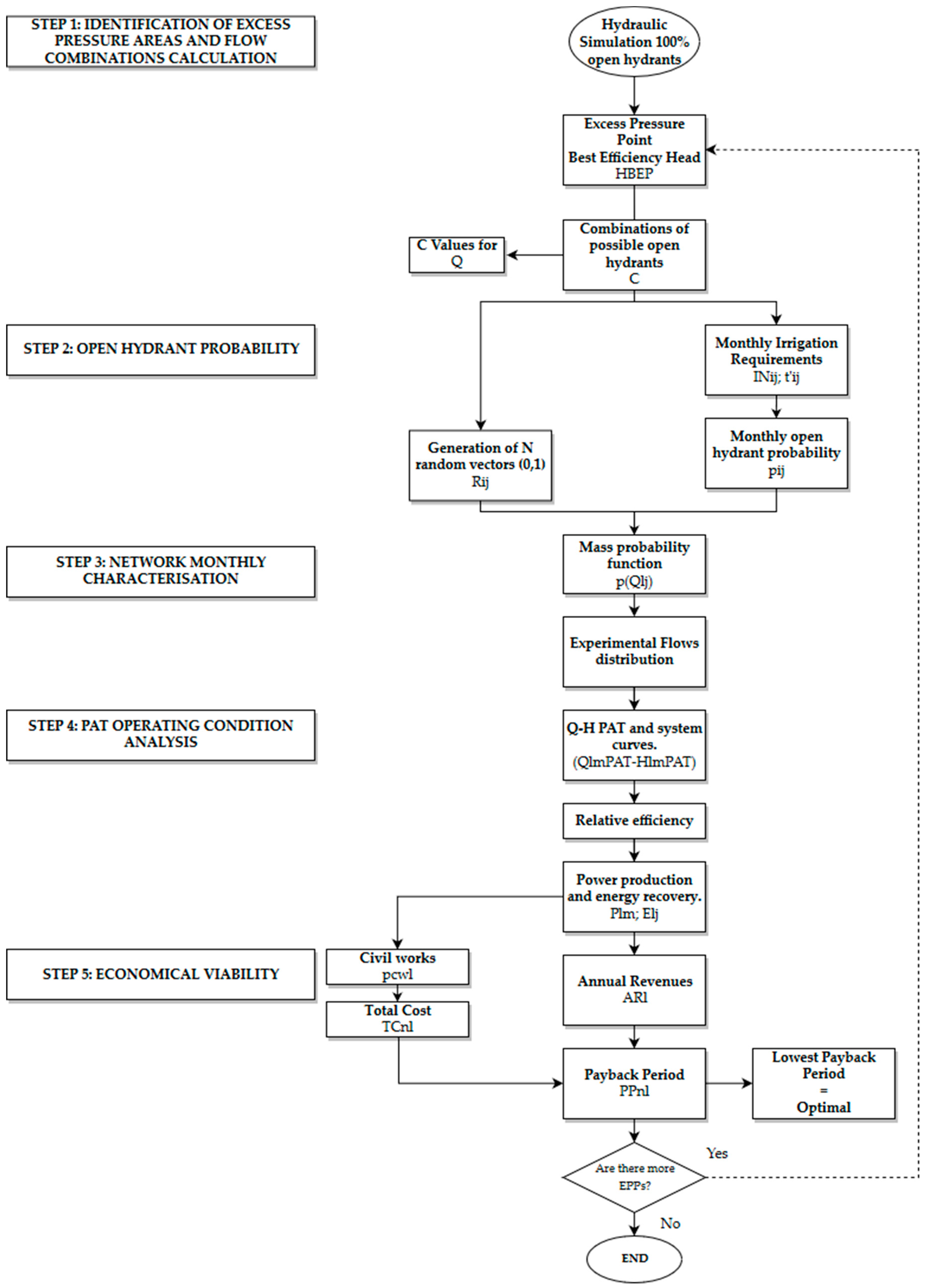
2.1. Methodology

The proposed methodology is based on the characterisation of the monthly behaviour of the network through a statistical experiment known as a Bernoulli Experiment. The experimental results define the value domain of the flow, considered a random variable Q , and their occurrence probabilities each month. The objective was to determine the PAT power for each selected Excess Pressure Point (EPP), while minimising the PAT installations payback period (PP). Experimental curves approximating the head recovered and the relative PAT efficiency, both depending on the flow rate together with the flow–head (Q–H) curve of the system, were used to estimate the power ranges and energy recovered. The methodology was defined as a general strategy for reducing the investment risks for PAT installation in irrigation networks. The methodology diagram can be seen in Figure 1 and is divided into five main steps, explained below:

2.1.1. Location of Excess Pressure Points and Calculation of Downstream Open/Closed Hydrants Combinations

The first stage in Figure 1 was to simulate the network’s hydraulic performance and find the excess pressure points along it, considering a pre-set hypothesis, such as design hypothesis or 100% of hydrants open. Within this first step, the next boundary condition was applied: BEP head ( H B E P ) is equal to the head available for each EPP in the first simulation under the hypothesis used, ensuring no lack of pressure in any scenario. H B E P had the same value for every scenario analysed within each EPP. Novara et al. [19] presented a Q-H space to locate the BEP conditions for a large set of PATs, showing several points where the head could reach up to 3 m for certain flows. Considering this space, the minimum head (excess pressure) for a point to be evaluated as an EPP was fixed at 3 m above the service pressure.
The flow fluctuations depended on the crop irrigated by each hydrant and their water requirements along the irrigation season. These fluctuations defined the values of the domain of the random variable Q , and was analysed through a Bernoulli Experiment. Hence, in each EPP, the range of possible values for Q was determined depending on the amount of possible combinations of downstream open/closed hydrants. Supposing a number of hydrants n , the number of possible combinations C , was calculated as defined by Equations (1) and (2), for a random combination of open hydrants a, with 0 a n . Finally, the Q-H curve for each branch to be analysed, was obtained from the hydraulic model. In the scheme shown in Figure 2, a random combination a for an EPP is represented.
C = ( n 0 ) + ( n 1 ) + ( n 2 ) + ( n n )
C a n = ( n a ) =   n ! a ! ( n a ) !

2.1.2. Open Hydrant Probability Calculation

This step aimed to calculate the monthly probability of each hydrant to be open. To obtain these probabilities, the formula proposed by Clément [27] was used. The distribution of crops irrigated by each hydrant and their monthly irrigation requirements were needed. For this, the method proposed by Allen et al. [29] was used through the CROPWAT software. Hence, the monthly water requirements matrix, I N i j (l ha−1 month−1), was obtained, with i referring to the hydrant and j to the month.
Clément defined that one hydrant has two possible working states: open, with a probability of p, and closed, with a probability of 1-p [27,30]. Thus, the monthly probability of an open hydrant ( p i j ), defined in Equation (3), was estimated as the relationship between monthly irrigation hours required by the crops, associated to each hydrant, t i j (hours month−1), and the monthly water availability, T i j (hours month−1) for each hydrant i in each month j. These were calculated following Equations (4) and (5), respectively. Finally, h o u r s i refers to the daily water availability (hours) per hydrant and d a y s j (days month−1) to the number of days in the month j. q m a x is the design flow allowed per unit of irrigated area.
p i j =   t i j T i j
t i j = 1 3600 I N i j q m a x
T i j = h o u r s i   d a y s j

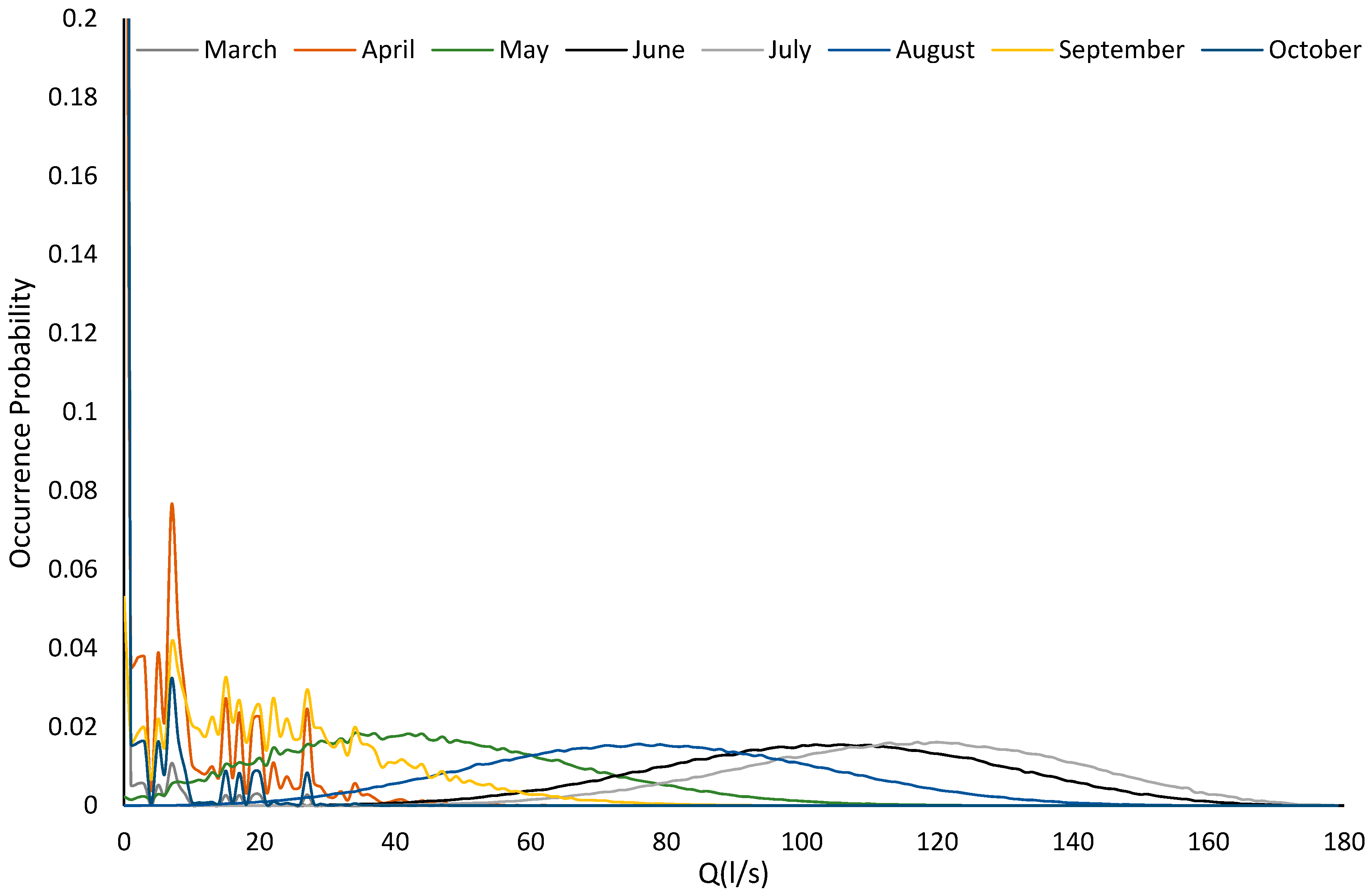
2.1.3. Monthly Characterisation of the Network: Mass Probability Function, p X ( x ) Calculation

The Bernoulli Experiment involved repeated independent trials of an experiment, called Bernoulli Trials (BTs), with two possible outcomes, arbitrarily called success (S) and failure (F) [31]. Knowing that the trials are independent and assigning the value 1 to S and 0 to F , the combinations of open and closed hydrants downstream of the EPPs were obtained, depending on the results of the trials. Therefore, every BT had two possible outcomes, X = 1 is understood as success, and the issue hydrant is open. On the other hand, if the result was X = 0 , then the result is failure and the issue hydrant is closed. Depending on the number of possible downstream open hydrant combinations (C), a number of BTs, N , is defined, since the greater the number of hydrants the greater the number of combinations, and so the greater the domain of Q . N will be at least double the number of combinations, in order to obtain every possible combination. Thus, every BT consisted of the generation of N random vectors, R i , with values between [0, 1], and its comparison with monthly probability of each hydrant to be open. The results obtained in each BT followed Equations (6) and (7):
I f   R i >   p i j X = 0
I f   R i   p i j X = 1 .
The aim of the BTs was to generate matrices with dimensions [N × j], which contained all the possible monthly values of the domain of the random variable Q , depending on the different combinations of open and closed hydrants. With these matrices, the behaviour of the network downstream of the EPPs could be characterized on a monthly basis.
The Bernoulli Experiment was run integrating the EPANET engine into Python (v. 2.7.15) through its Dynamic Link Library (DLL). Bernoulli distributions were obtained after each trial. These distributions are directly related with binomial distribution. Binomial distribution is defined by the number of independent trials carried out, N, and the probability of success, p. When the number of trials is 1, then the binomial distribution is called a Bernoulli distribution. Therefore, the results obtained for every EPP composed the domain of Q . Analysing these results, the monthly flow values and their occurrence probability could be calculated. Hence, for each EPP, 12 (monthly) binomial distributions were obtained.
The probability mass function of a discrete random variable X conveys the same information as a table of probabilities of simple events for the possible values of X [31]. Thus, after calculating every possible flow value Q l , the next step was to calculate how often these values occur monthly. The mass probability function for the whole domain was obtained dividing the times, n l j , that each value Q l was repeated in each month j, by the number of total BTs (N). The occurrence probability of each flow value was obtained following Equation (8):
p ( Q l j ) = n l j N .
A comparison between the monthly experimental volume and the monthly theoretical volume required was made in each EPP. Its aim was to check how good the experiment fitted with the theoretical values. To calculate the monthly experimental volumes per unit of irrigated surface, the monthly flow distributions and their probabilities were required. Applying Equation (9), the monthly experimental volumes were calculated as:
E V j = 3600   T i j q m a x q M l = 1 C Q l   p ( Q l j ) ,
where E V j is the monthly experimental volume; q m a x is the design flow allowed per unit of irrigated area; q M is the maximum flow circulating through the EPP.

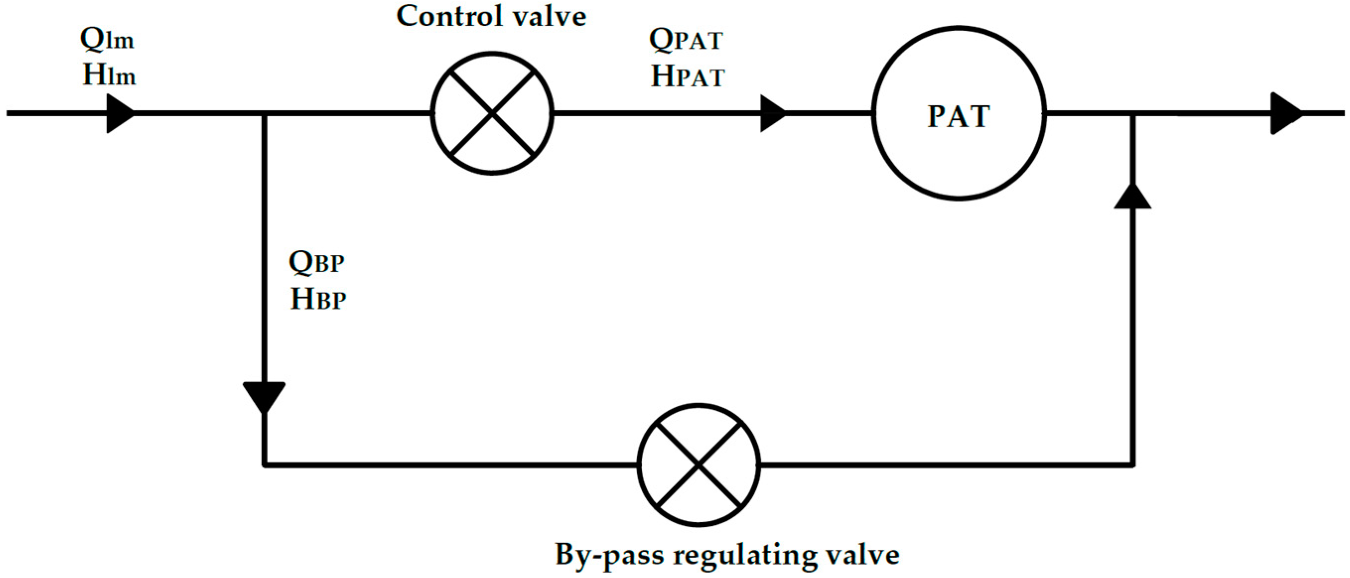
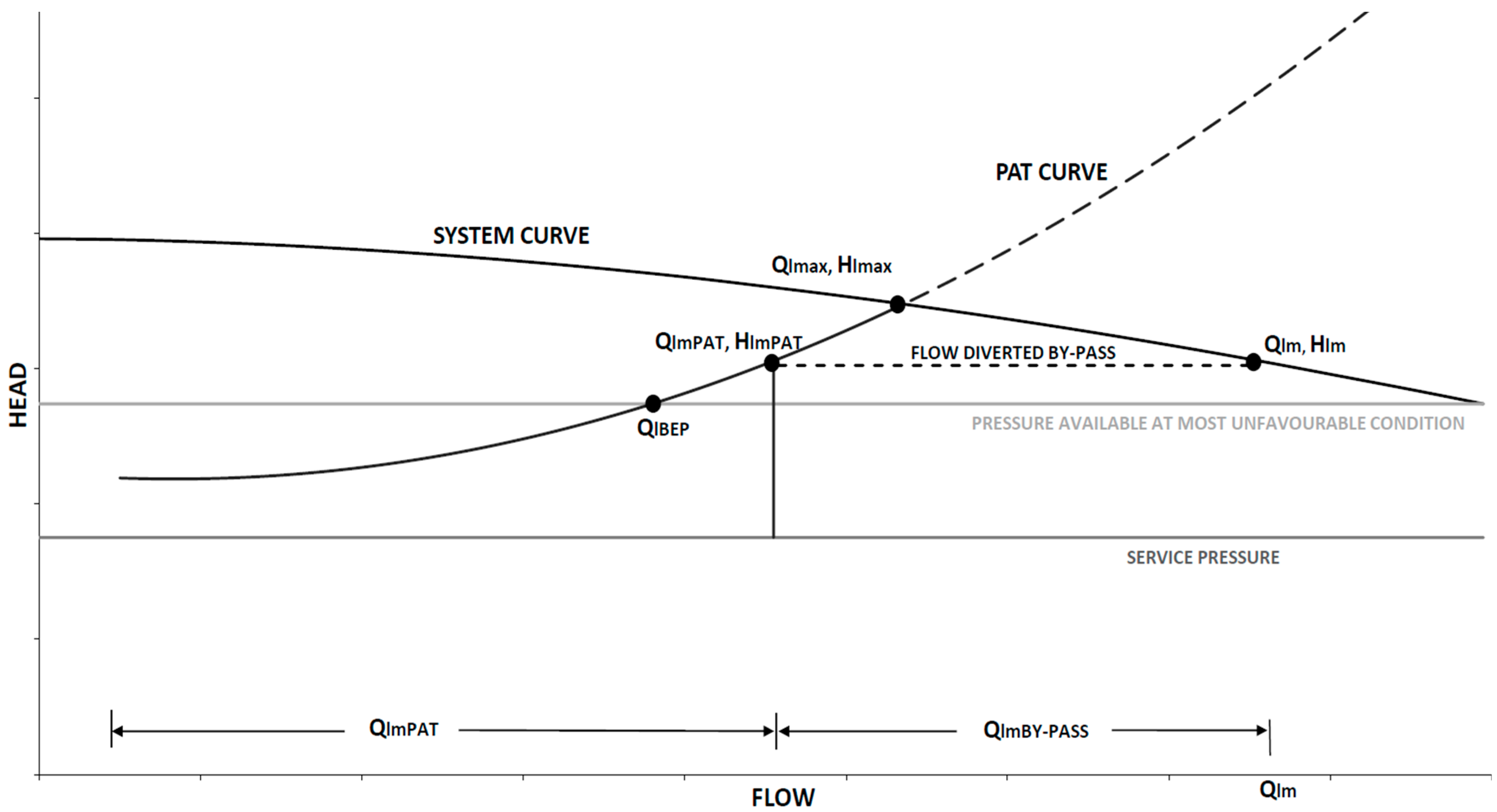
2.1.4. PAT Operating Conditions Analysis

Every possible flow circulating through the EPP pipe was considered as a possible BEP flow of a theoretical PAT. Hence, l different scenarios were defined, each of them corresponding to one PAT, whose BEP was ( Q l B E P ,   H B E P ). To regulate the PAT inlet conditions and keep the network service conditions downstream, the bypass scheme proposed by Lydon et al. [32], has been considered, in which there are two control valves, one before the PAT and the other in parallel. The regulation used was hydraulic regulation (HR), since previous investigations concluded that HR is generally more efficient than electric regulation, showing larger efficiencies when the working conditions vary from the design values. In addition, they were also shown to be less expensive [13]. This can be observed in Figure 3.
The methodology followed to estimate the flows running through the turbine, simulated the interaction between the Q–H system and PAT curves. The two operating rules fixed were: (i) the flow demanded downstream of the EPP would fully circulate through the turbine if its value is lower than or equal to the maximum flow to be turbined Q l M A X in each scenario l (This value was calculated obtaining the intersection between both, PAT and system Q-H curves); (ii) if the flow demanded downstream is greater than the maximum fixed for each scenario Q l M A X , this flow would be diverted to the bypass. To obtain the amount of flow diverted in each scenario l for each flow demanded downstream m, Q l m B P , the interaction between both system and PAT curves is required again.
Operating Rules:
(i)
i f Q l m Q l M A X { Q P A T = Q l m Q l m B P = 0 }
(ii)
i f Q l m > Q l M A X { Q P A T = Q l m P A T Q l m B P = Q l m Q l m P A T }
The methodology assumes that the selection of a pump to operate as a turbine with the specified BEP can be carried out independently, using the approaches described in Lydon et al. [32]. The method then adopts the approach proposed by Barbarelli et al. [32] to estimate the PAT characteristic curves (head & flow). Barbarelli, proposed an alternative curve to the curve suggested by Derakshan and Nourbakhsh [33], to obtain the relative head for any given machine, based on 12 pumps tested as turbines. This curve followed Equation (10). Thus, all the relative heads were obtained for every flow demanded downstream Q l m in the scenario l. The value of the head recovered by the PAT H l m was calculated multiplying the relative heads by the BEP head, H B E P . With these heads quantified for every PAT associated to every scenario l, all the Q-H curves for the specific system were obtained. These equations had the form of Equation (11), where the coefficients changed for each hypothetical PAT tested:
H l m H B E P = 0.922 ( Q l m Q l B E P ) 2 0.406 ( Q l m Q l B E P ) + 0.483
H l m P A T = a Q l m P A T 2 + b Q l m P A T + c ,
where H l m P A T is the head recovered for a certain flow Q l m P A T running through the PAT. In Figure 4, this interaction and intersection between a potential PAT and the system curve for a random site is displayed. To calculate the amount of flow turbined and the amount diverted through the bypass, every possible flow value greater than Q l M A X , was introduced in the system curve, obtaining the head available ( H l m S y s t e m ) in the system for such a flow ( Q l m ) . Using this head ( H l m S y s t e m ) in the PAT curve as the head recovered ( H l m P A T ) , the flow circulating through the PAT was fixed. Applying this sequence to every possible flow greater than Q l M A X , all the pairs ( Q l m P A T ,   H l m P A T ) , for which the device could work, were calculated. Consequently, in scenario l, the portion of flow diverted through the bypass for values greater than Q l M A X was the difference between the flow demanded downstream and the flow turbined ( Q l m Q l m P A T ) .
Each of these pairs ( Q l m P A T ,   H l m P A T ) had an associated relative efficiency, under which the PAT operates. Novara et al. [34] proposed a model, through the extrapolation 116 measured PAT characteristic curves, estimating the behaviour of their relative efficiency depending on the flow rate. Thus, the mechanical relative efficiency was obtained for each flow, Q l m P A T , in scenario l, following Equation (12). As a conservative estimate the maximum efficiency was fixed at 55% (0.65 PATs + generator efficiency and 0.85 to take into account the hydraulic regulation losses) [12]. For very low flow rates, this relative efficiency has negative values, for which the device should be off or the flow would be diverted. The power production for each scenario l, whose BEP is ( Q l B E P ,     H l B E P ), for each pair ( Q l m , H l m ), was obtained as per Equation (13). For very low flow rates, this relative efficiency has negative values, for which the device should be off and no flow would be turbined.
η l m = 0.5197 ( Q l m P A T Q l B E P ) 3   2.3328 ( Q l m P A T Q l B E P ) 2 + 3.0931 ( Q l m P A T Q l B E P ) 0.2757
P l m = 0.55   Q l m P A T   H l m P A T   γ   η l m
where Q l B E P is the value of the BEP flow for each scenario l; γ is the specific weight of the water; η l m is the relative efficiency value for each pair for scenario l. Lastly, to estimate the monthly energy recovered, the powers produced by each PAT for each pair ( Q l m P A T ,   H l m P A T ) in scenario l were used, together with the monthly mass probability function and the monthly available time. The monthly available time matrix was reduced to a single vector, since it was an on-demand irrigation network, where every hydrant had 24 h availability every day of the year. Its calculation followed Equation (14):
E l j = P l m   p ( q l j )   T j .

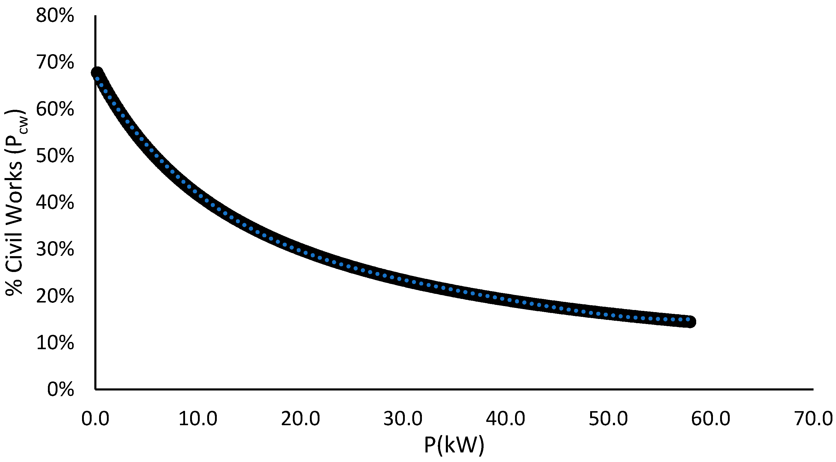
2.1.5. Economic Viability
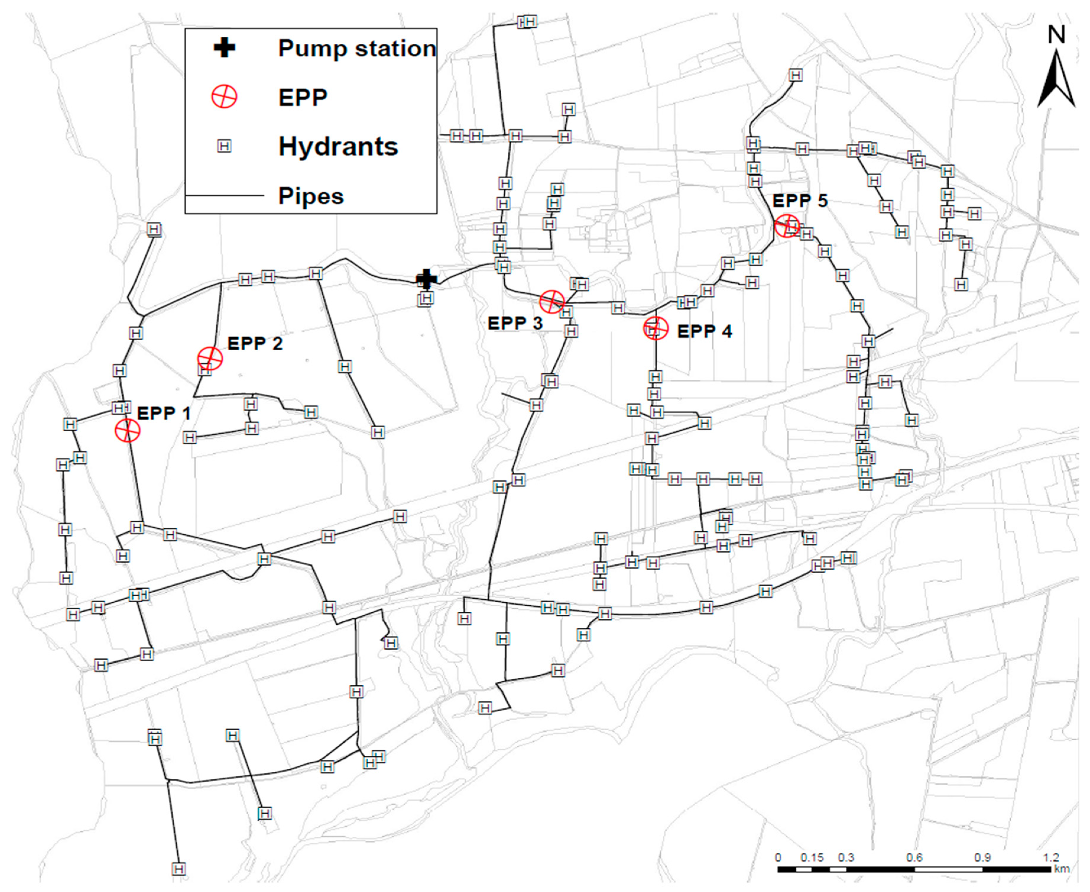
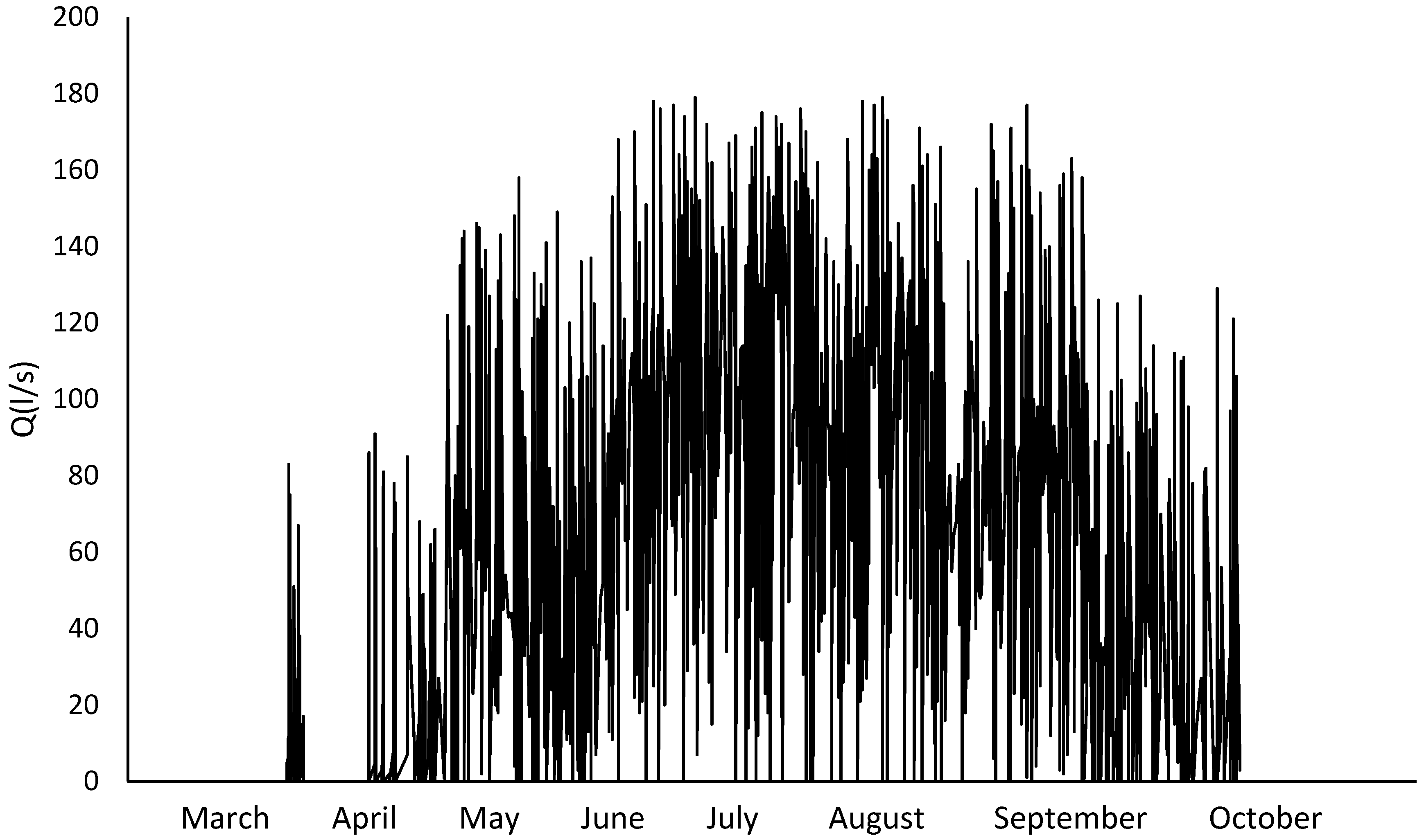
The last stage of the methodology was to assess the economic viability of each scenario studied. Payback Period (PP) was used here to determine the period needed to recover the investment made, neglecting the time value of money.
To quantify the total installation cost, three different main components have been considered: electromechanical (PAT + generator), civil works and additional works. Regarding the electromechanical part, different investigations have given different approaches. Ramos et al. [15] estimated the cost of a PAT to vary between 200–400 €/kW for nominal power lower than 40 kW. Carravetta et al. [13] proposed the sum of nominal power of the turbine, 230 €/kW, and the maximum PAT power accounting for the cost of the generator, 115 €/kW. De Marchis et al. [35] proposed a cost per power unit of 2000 €/kW for PAT plus generator. In this research, a cost model, which estimates the unitary price for PAT and generator, has been used. This model estimates different kinds of radial PATs, including generator with one, two or three pairs of magnetic poles (pp) [19]. The cost per kW of the centrifugal PATs coupled with induction generators with the number of pp mentioned is related to the parameter Q l B E P H B E P . Thus, the electromechanical cost has been calculated for every possible BEP flow value and the BEP head was fixed, using Equations (15)–(17):
C P P 1 l = 11 , 589.32   Q l B E P H B E P + 1380.79
C P P 2 l = 12 , 864.77   Q l B E P H B E P + 949.43
C P P 3 l = 15 , 484.97   Q l B E P H B E P + 1172.72 .
In addition to the PAT costs, other works have to be added, such as civil work and the cost of the bypass. Regarding the civil works, a new approach has been developed within this research, explained in Appendix A. The percentage of the civil works costs depending on the power installed was calculated using Equation (18), proposed in this research. For additional works, such as electric connection or maintenance, 20% of the total costs has been considered. Following Equation (19), the total costs for the installations were obtained as:
p c w l = 1 · 10 7 P l B E P 4 2 · 10 5   P l B E P 3 + 0.0011   P l B E P 2 0.0349   P l B E P + 0.6714
T C n l = C C P P n l ( 1 p c w l )   0.8 ,
where p c w l is the percentage of the civil works over the total installation cost in scenario l, and C P P n l is the total installation cost for each flow value and number of polar pairs, n, of the electromechanical devices. To complete the economic analysis, the calculation of the annual revenues (AR) and the PP was carried out. For the first term, the total energy produced in each scenario has been multiplied by the income rate, in case of selling to the grid, or the energy tariff in case of auto consumption. This rate will depend on the country where the installation is made. Thus, applying Equations (20) and (21) the AR and PP for each scenario was calculated:
A R l = j = 1 12 E l j r j
P P n l = C P P n l A R l ,
where E l j is the monthly energy recovered in each scenario l; the vector r j represents the money received or saved per kilowatt every month. Finally, analysing all the PPs associated to scenario l and every potential PAT, n, the selected scenario would be the one whose PP is the lowest, considering the respective BEP power to be installed. It has to be highlighted, that for MHP technology, the PP has to be lower than 10 years [14] to be considered economically viable in the water sector. Thus, of all the points studied, those with P P 10   years were discarded.

2.2. Study Area

Sector VII of the right bank of the Bembezar River (BMD) is a pressurized water distribution network located in Seville (Spain). The network is composed of pipes with diameters between 150 and 800 mm. It contains 162 hydrants that irrigate a total surface of 920 hectares. The main crops cultivated in the district are: citrus (56%), maize (32%), cotton (9%) and sunflower (3%) [36]. The hydrants are distributed in levels that vary between 47 m and 97 m.
A pumping station is located at 86 m.O.D (meters above the ordenance Datum). and is composed of two kinds of pumps. The first type has a power of 90 kW, and there are three of these units. The second type has a power of 270 kW, and there are two of these units. The network was designed to supply 1.2 l/s/ha on demand, so water is continuously available to farmers (24 h per day). The network was designed for 100% of open hydrants simultaneity. The methodology has been applied for the 2017 irrigation season, for which the agronomic parameters (rainfall and evapotranspiration) have been considered. The values of these parameters for the 2017 irrigation season were 440 mm and 1210 mm, respectively.

3. Results

3.1. Location of Excess Pressure Areas and Calculation of Downstream Open/Closed Hydrant Combinations

In this first stage, hydraulic simulation following the design hypothesis, 100% of the hydrants of the network set as open, was conducted, using EPANET [37]. As a result, five points have been identified as potential EPPs, with an available excess pressure of 19.1 m, 13.9 m, 19.8 m, 18 m and 14.3 m, respectively. In this first assessment, the BEP head for the turbine was fixed, since the first simulation has been carried out under the most unfavourable conditions. In this way, it was ensured that the service pressure reaching the hydrants located downstream was always greater than or equal to the minimal pressure required, 35 m in this case. The location of these points can be seen in Figure 5, noting that each EPP was located on a separate branch of the network.
The number of hydrants located downstream of each EPP was then counted, to obtain the number of possible open hydrant combinations, following Equations (1) and (2).

3.2. Open Hydrant Probability Calculation

As there is no record available of the actual open hydrant time, it has to be estimated by means of the formula proposed by Clément (1966) [27]. Regarding the crop distribution, the crops irrigated by each hydrant were also not available, and just the percentage of total land for each crop was known. Therefore, this general distribution has been applied to each hydrant. These two first steps of the second stage could be replaced by actual information in case the irrigation network studied had these data available. Thus, firstly, the monthly crop water requirements were calculated. The required irrigation time per hydrant and month was then calculated using Equation (4). Specifically, this network is an on-demand irrigation network, so the water availability is 24 h every day. Then, the monthly probability of open hydrant was calculated for each hydrant using Equation (3). Since the crop distribution per hydrant was not available, the general percentage of crops mentioned in the description of the case study has been applied to each hydrant, assuming all of them had the same open hydrant probability, as shown in Table 1. The characteristics of each EPP before running the experiment and the input information are shown in Table 2.

3.3. Monthly Characterisation of the Network: Mass Probability Function, p X ( x ) Calculation

Once the monthly open hydrant matrices were defined for every hydrant of the network, several BTs were run, in order to characterise the behaviour of the network across the year. Thus, analysing the results obtained for each EPP it can be seen that the flow values varied from 0–297 l s−1, 0–82 l s−1, 0–179 l s−1, 0–101 l s−1 and 0–75 l s−1, respectively. From these results, a distribution of the flows along the irrigation season was obtained, and the monthly behaviour of the network could be characterised by analysing the 12 monthly binomial distributions. The mass probability functions were calculated using Equation (8).
In Figure 6 the mass probability functions corresponding to the months of irrigation season for EPP3 can be seen. The mass probability function illustrates the monthly occurrence probability of every flow of the domain of Q . Thus, in Figure 7 it can be seen how the occurrence probabilities change along the months represented. Higher probabilities can be seen for lower flows in months where the irrigation requirements are lower, and higher probabilities for greater flows in months with more irrigation requirements. The >60 million experimental flows obtained for the irrigation season are displayed for EPP3 in Figure 8.
The monthly experimental volumes were calculated using Equation (9). The variations between the theoretical and experimental values for EPP3 can be seen in Figure 9. The annual variations found between the theoretical and experimental volumes in the five EPPs were −0.0873%, 0.3867%, 0.0816%, −0.08024% and 1.2287%, respectively.

3.4. PAT Operating Conditions Analysis

Every experimental Q-H and PAT curve had to be defined. Every Q-H system curve was obtained from the hydraulic model. For the different EPPs, an average of 16 million experimental curves were tested per EPP using Equation (10). Calculating the intersection between every PAT curve and the system curve, the maximum flow allowed to run through each device was obtained in each scenario l. Once these maximum flows were defined, the space of ( Q l m P A T ,   H l m P A T ) for each PAT associated to each scenario l were also defined for each possible value of Q . The relative efficiencies that every pair of ( Q l m P A T ,   H l m P A T ) would produce in each PAT were calculated using Equation (12), depending on the BEP flow of each device. With all the flows and heads for which the PATs would operate under, and the relative efficiencies associated to these values, the power produced in each circumstance was estimated.

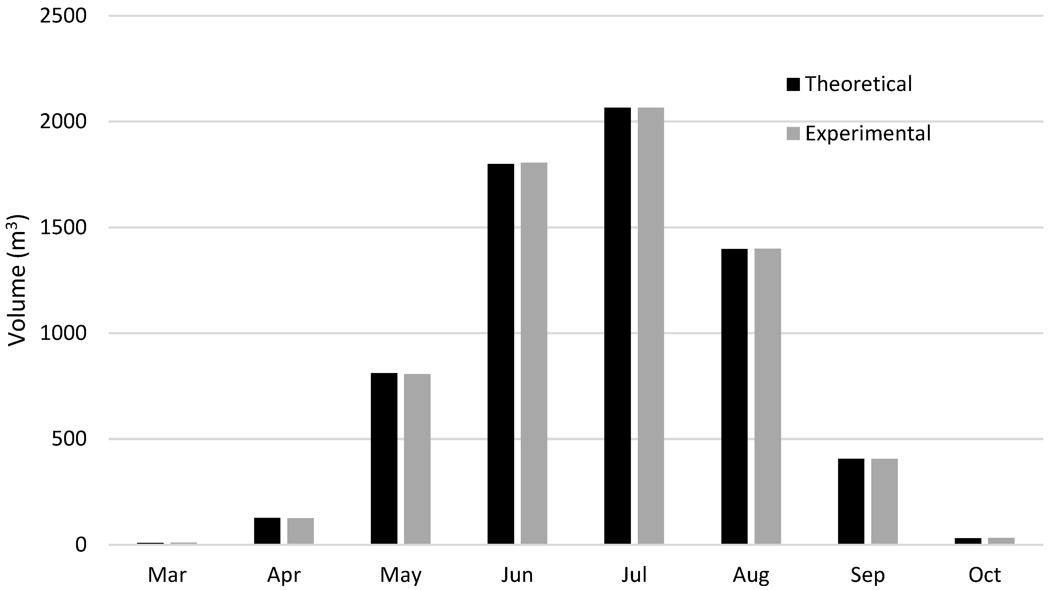
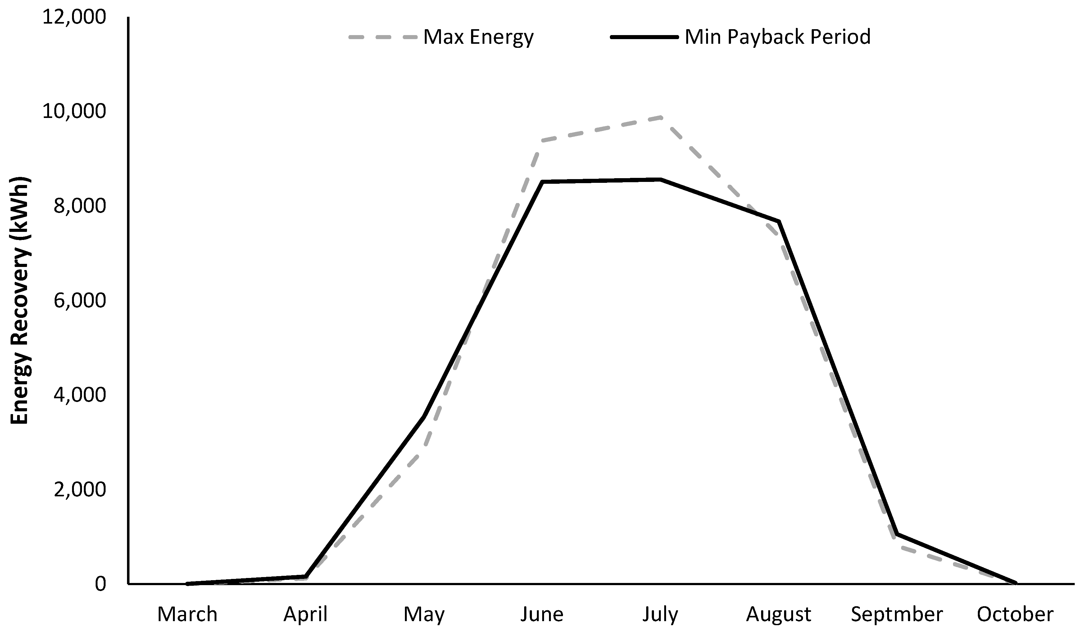
3.5. Economic Viability

The cost associated to each scenario and every PAT evaluated was calculated using Equations (15)–(17). To estimate the civil works associated to each scenario, Equation (18) was applied. Depending on the power, the percentage represented by the civil works varies from low values, close to 10% of the total installation cost for greater powers, up to high values close to 70% for lower powers.
For the five EPPs analysed in the network studied, the energy that would be recovered varies within the range 0.9–43.3, 2.4–6.9, 1.1–30.4, 0.5–11.2 and 0.4–5.6 MWh, respectively. To calculate the annual revenues, several authors have used different values in their research. Perez-Sanchez et al. [23] fixed a price of 0.0842     kWh 1 , whilst Garcia Morillo et al. [22] applied the monthly average of the Spanish tariff based on six periods. In this case, the application LUMIOS (REE, 2014) [38], developed by the Spanish Electrical Grid, which provides the monthly average tariff for a selected period, has been used to calculate the monthly tariff for 2017.
The values, in   kWh 1 , for the months in which energy is produced, were: April (0.111242), May (0.112542), June (0.113439), July (0.113044), August (0.113056) and September (0.113611). These tariffs were considered since the energy recovered has been assumed to be for self-consumption instead of selling it to the grid, as in many cases, there are no grid connection points close to the installation and it would be considered as saved energy. Thus, this connection could make the installation much more expensive, and was not considered as a viable solution for energy production in the irrigation sector.
Using Equations (20) and (21) to calculate the annual revenues and the payback period, respectively, for each scenario, and following the boundary conditions imposed for the payback period, the optimal PAT for each EPP was obtained, or the EPP was rejected. Thus, for the five EPPs, the summarised results can be seen in Table 3. Two of them were considered as viable individually for a PAT installation for energy recovery, two of them were rejected because of their PP exceeded 10 years, and one could be considered as potentially viable for being just in the border of the 10 years for returning the investment. These three EPPs would recover a sum of 81.4 MWh. Nevertheless, considering the five EPPs as a single investment, the PP would be 6.4 years, increasing the energy recovered to 93.9 MWh for the whole set.
The civil works, which were calculated following Equation (20), for the optimal solution of each EPP represented 43.5%, 58%, 50.3%, 53.5% and 58.2% of the total cost, respectively.

4. Discussion

Flow fluctuations are very significant in irrigation networks, since the irrigation requirements vary along the irrigation season, depending on the crops. Furthermore, the farmers’ irrigation habits are not standardized in on-demand irrigation networks. Due to the difficulty of accessing data in this sector, one method to obtain the performance of the network is a statistical analysis based on the crop water requirements. Applying Clément’s methodology and Bernoulli Experiments to an on-demand irrigation network, an estimation of the data along the network can be obtained. Characterising the network through their application makes the estimation of the flow fluctuations possible, approximating the monthly probability that each flow has of occurring and the probability to be exceeded. This analysis estimated the different values that could run through a specific pipe during the whole irrigation season. All of these flows have been evaluated as BEP flows simulating as many theoretical PATs as the number of flow values there were for each EPP. However, only one machine can be selected for installation, and this methodology allows us to select a PAT whose BEP gives the best return on investment from all possible flow/head combinations across the irrigation season.
A limitation of this methodology is that a general PAT performance curve has been considered for all of the possible PATs that could be installed, underestimating in some cases and overestimating in others, the energy that could be recovered using each specific PAT studied. This general performance curve has been developed from the characteristic curves of 116 different PATs, extrapolating them and obtaining a general curve [34]. Therefore, this methodology, applied to the general PAT performance curve, helped us to study all the possible scenarios for an energy recovery installation, pre-selecting the possible power outputs and choosing the best one for the payback period. However, a deeper investigation would be necessary in each EPP site once it is established by this methodology that the economic viability is predicted to be favourable.
Another limitation of the methodology is the fact that while many theoretical PAT BEPs were analysed among the possible combinations of flow across the irrigation season, a finite number of pumps exist in the market. The PAT curves were obtained using Equation (10), which is based on experimental data from 12 pumps tested as turbines [32]. In reverse these pumps function as PATs and are considerably cheaper than traditional turbines due to mass production. Therefore not every theoretical PAT is in existence in the marketplace and to retain cost-competitiveness, in practice we would need to select the closest available machine to the selected theoretical one for a specific EPP. The current methodology may under- or over-estimate economic viability at specific EPPs as a result of this limitation.
Regarding the domain of the random variable Q , formed by the number of possible combinations of downstream open and closed hydrants, it will be greater as the number of downstream hydrants increases. This means that the possible flow values will increase as the number of downstream hydrants does, having a larger probability of flow fluctuations as the quantity of hydrants increases. In the present case study, four of the EPPs had more than 20 hydrants downstream, where, >2 million possible flows could occur.
The consideration of relative efficiencies in this paper are very important. For the flow fluctuations, as their occurrence probabilities change significantly along the irrigation season, the energy that would be produced using other methodologies that just account for the energy recovered under BEP for average flows and heads, would not give realistic results. Thus, the variation of the PATs efficiency depending on the flow rate variation, allows a more realistic power output capacity to be installed in a specific EPP. Different variables could be considered when the viability of a PAT installation is being examined, such as the energy maximization. Nonetheless, if the variable to be maximised was the energy, then, the optimal scenarios would divert to higher BEP powers, where the PP would rise to levels that could make the investment unviable. In spite of this, maximising the energy has been used in other research, and this methodology selects the best PAT for which the investment would be recovered the soonest. This would be more inviting for farmers to install.
A comparison between the energy recovered in the scenario with the lowest PP and the scenario producing the greatest energy is displayed in Figure 9 (EPP3). The energy would increase up to 30.2 MWh. This would amount to 2.3% more energy recovery. However, the PP would increase by 4.4%.
The civil works accounted for here differed from the civil works used by other authors. Some authors stated that 65% of the total installation corresponded to the cost of the PAT and the generator, and the other 35% was accounted for other works [39]. In other cases, the civil works were considered to be around 25% of the total installation costs [21]. Both considerations linked the civil work costs to the power to be installed and many previous papers were also not considering costs in the irrigation setting. Nonetheless, for a random installation, the percentage of costs represented by civil works will change with the power. Thus, different power values of PAT for the same point will not change the civil works to be conducted, but the percentage of these will change, being lower as the power increases. Therefore, for this research, an estimation of the general civil works to be carried out in these kind of installations in irrigation networks has been calculated, which contains general works and the main elements to be carried out. The result is a curve relating the power of the installation with the percentage represented by the civil works within the total costs of the installation. This gives a more realistic weight to the civil works than the previously used.
The energy prices to be considered depend on the location of the irrigation network and energy use. In this case, the energy recovered has been considered to be auto-consumed by the farmers or the irrigation district itself. Hence, the energy recovered could be considered as a savings on the energy consumption.
The case studies pump station accounts for a power consumption of 1080 kW. The power estimated to be potentially viable, was 25.1 kW. This amount represents 2.3% of the total power of the pump station. However, the power production of 25.1 kW represents the average power output across the year, where peak production of up to 45.8 kW would be reached in some stages of the irrigation season. The five PATs would be able to recover 93.9 kWh in an irrigation season. If the nominal power of the whole set is compared with the unitary pumps’ power, the PATs’ power amounts to 28.0% of the total power for the first type and 9.3% for the second type. Depending on the stage of the irrigation season, the number of pumps working changes. Therefore, this could translate to an important energy savings in those stages where a lower number of pumps work. The index of the annual energy recovered per irrigated surface area was 0.10 MWh year−1 ha−1. This shows that the potential available in this specific network is not large. Previous investigations showed values of 0.65 and 0.08 MWh year−1 ha−1 [22,23]. However, these values cannot be compared, since each index will partially depend on the topography in which the network is built. In addition, previous estimates did not considered both flow variations and turbine efficiency variations.
Finally, the application of MHP for energy recovery together with other potential energy saving measures proposed in other investigations would have a positive effect, reducing the energy dependency of the activity. For instance, the optimisation of pump stations would not remove the excess pressure in every area of a network. The excess pressure due to change in elevation, among others, would still exist, and therefore the application of MHP would be a viable solution for both reducing the excess pressure and energy dependency in the network.

5. Conclusions

The use of renewable energy sources in the agricultural sector will increase in the next few years. The percentage of crop water costs related to the energy comprises an important percentage of the total costs paid by farmers. In addition, the environmental pressure to reduce the greenhouse gases emissions will be a critical driver in this issue. PAT installations in these infrastructures have been shown to be viable solution to improve the sustainability and economic viability of this sector, due to their low cost in comparison with other technologies such as traditional turbines in the case of hydropower.
Reducing operating costs by this amount will result in lower food prices for consumers and potential for greater crop yields (avoiding deficit irrigation). As a result, the incorporation of MHP energy recovery in irrigation networks has an important role to play in the water‒energy‒food nexus, lowering GHG emissions, lowering food prices, reducing energy consumption and increasing crop yields.
This research develops a new methodology to optimise the PAT power to install at pre-selected sites in irrigation networks, where no data are recorded, minimising the payback period of the investment and combining combinatorial and statistical analysis. Three constraint conditions were fixed to achieve this goal. There can be no lack of pressure in the network after the installation with these constraints applied. The installation PP had to be lower than 10 years. Moreover, the scenario with the lowest PP was selected, whose power is the basis of the PAT selected.
The energy recovery for the set including the five EPPs, summed to 93.9 MWh. The energy savings estimated in this paper could comprise important economical savings for farmers. Future works will study the validation of this methodology with actual measured data, and its use in irrigation networks where there is no access to actual data, to assess the potential in this sector and the percentage represented by energy saved over the total energy consumed.

Author Contributions

All authors have participated in every step of this research. J.A.R.D. and J.G.M. provided information about the irrigation networks and supervised the probabilistic approach and hydraulic analysis. M.C.C. proposed the methodology to minimize the payback period and reduce the risk investment as well as the methods and materials used. A.M. supervised the research and document preparation.

Funding

This research was partially funded by the European Regional Development Fund (ERDF) through the Interreg Atlantic Area Programme 2014–2020, as part of the REDAWN project (Reducing the Energy Dependency in the Atlantic Area from Water Networks), and the Spanish Ministry of Economy and Competitiveness through the AGL2017-82927-C3-1-R Project.

Conflicts of Interest

The authors declare no conflict of interest. The funders had no role in the design of the study; in the collection, analyses, or interpretation of data; in the writing of the manuscript; or in the decision to publish the results.

Abbreviations

a Random scenario
A R l Annual revenues generated for the installation designed for the flow l
B T Bernoulli Trial
C Combinations of downstream open hydrants
C P P n l Total cost for a PAT with n magnetic polar pairs generator installation for the flow l
d a y s j Monthly days
E V j Monthly experimental volumes
E l j Monthly energy recovered in the scenario l
H B E P Best efficiency point head
H l m P A T Head recovered for flow m in scenario l
I N i j Monthly water requirements per hydrant
N Number of simulations
n Number of downstream hydrants
n l j Monthly number of repeating times of the flow value l
p i j Monthly open hydrant probability
P l m Power for the scenario produced for the inlet flow m in the scenario l
p X ( x ) Mass probability function
p ( q l j ) Monthly mass probability function of the flow value l
p c w Percentage of civil works in the total installation cost
P P n l Payback period for an PAT installation design for the flow l with a generator with n polar pairs
q m a x Design flow of the network
q M Maximum flow running in the pipe EPP studied
q l Value of the flow in scenario l
Q Random variable Flow
Q l B E P BEP flow value in scenario l
Q l m P A T Flow running through the PAT when m flow is demanded in the scenario l
R j Monthly random vector [0-1]
r j Monthly energy tariff
t i j Monthly hydrant irrigation time required
T i j Monthly hydrant water availability
η m a x Maximum PAT performance
η l m Relative performance of the flow value m in the PAT designed for flow value l
γ Water specific weight
Sub-indexes
i Hydrant sub-index
j Month sub-index
l Flow values for main scenarios sub-index
m Flow values for relative scenarios sub-index
n Generator magnetic polar pair sub-index

Appendix A

This appendix contains a description of the civil works considered in this research. Previous investigations stated that the civil work costs could be taken into account as a fixed percentage of the total installation, independent of the PAT costs and power. This consideration does not match reality since the civil works to be made will depend on the power to be installed, and the cost. Therefore, for general cases, the percentage represented by the civil works would depend on the power of the PAT, or rather, the PAT cost. The method proposed in this paper is based on the estimation of the parties that would be involved in a general PAT installation in irrigation networks. Concrete foundation for the PAT, earthworks, materials and construction of the bypass, backfilling and protection house have been considered as general parties for a general PAT installation in these infrastructures. In some cases, the parties involved would be more expensive. Nonetheless, this approach provides a better estimation of the civil works, since they will be almost the same for any specific point, independently of the power to be installed. Thus, it can be said that the lower is the power the higher percentage will be represented by the civil works in the total costs. A brief bill of quantities (BOQ), whose unitary prices have been fixed from the Spanish Price Generator for Construction Database [40], is given in Table A1. From this BOQ, which shows the percentage represented by the civil works over the total installation costs, Figure A1 has been developed.
Table A1. Summary of the parties accounted in the civil work costs.
Civil Works
CW.1Manual trench excavation (20 × 2 × 1.5 m)m37649.45 3758.20
CW.2Bypass: Supply + fixing 300 mm ductile iron pipes lm1896.35 1734.30
CW.3Reinforced concrete slab 10 cmm28€16.2 €129.8
CW.4Protection House: Concrete blocks (40 × 20 × 10 cm) supply and fixing (4 × 2 × 2.5 m)m230€41.78 €1253.40
CW.5Manual backfilling: Same material excavationm376€3.54 €269.04
Total €7144.78
Figure A1. Cost percentage represented by the civil works depending on the PAT power.
Water 11 00149 g0a1

References

  1. Nogueira, M.; Perrella, J. Energy and hydraulic efficiency in conventional water supply systems. Renew. Sustain. Energy Rev. 2014, 30, 701–714. [Google Scholar] [CrossRef]
  2. Copeland, C.; Carter, N.T. Energy-Water Nexus: The Water Sector’s Energy Use; Congressional Research Service: Washington, DC, USA, 2017.
  3. Lofman, D.; Petersen, M.; Bower, A. Water, Energy and Environment Nexus: The California Experience. Int. J. Water Resour. Dev. 2002, 18, 73–85. [Google Scholar] [CrossRef]
  4. Rodríguez-Díaz, J.A.; Pérez-Urrestarazu, L.; Camacho-Poyato, E.; Montesinos, P. The paradox of irrigation scheme modernization: More efficient water use linked to higher energy demand. Span. J. Agric. Res. 2011, 9, 1000–1008. [Google Scholar] [CrossRef]
  5. Navarro Navajas, J.M.; Montesinos, P.; Camacho-Poyato, E.; Rodríguez-Díaz, J.A. Impacts of irrigation network sectoring as an energy saving measure on olive grove production. J. Environ. Manag. 2012, 111, 1–9. [Google Scholar] [CrossRef] [PubMed]
  6. Moreno, M.; Corcoles, J.; Tarjuelo, J.; Ortega, J. Energy efficiency of pressurised irrigation networks managed on-demand and under a rotation schedule. Biosyst. Eng. 2010, 107, 349–363. [Google Scholar] [CrossRef]
  7. Fernández García, I.; Rodríguez Díaz, J.A.; Camacho Poyato, E.; Montesinos, P. Optimal operation of pressurized irrigation networks with several supply sources. Water Resour. Manag. 2013, 27, 2855–2869. [Google Scholar] [CrossRef]
  8. Pardo, M.A.; Manzano, J.; Cabrera, E.; García-Serra, J. Energy audit of irrigation networks. Biosyst. Eng. 2013, 115, 89–101. [Google Scholar] [CrossRef]
  9. Jimenez-Bello, M.A.; Royuela, A.; Manzano, J.; Prats, A.G.; Martínez-Alzamora, F. Methodology to improve water and energy use by proper irrigation scheduling in pressurised networks. Agric. Water Manag. 2015, 149, 91–101. [Google Scholar] [CrossRef]
  10. Mérida García, A.; Fernández García, I.; Camacho Poyato, E.; Montesinos Barrios, P.; Rodríguez Díaz, J.A. Coupling irrigation scheduling with solar energy production in a smart irrigation management system. J. Clean. Prod. 2018, 175, 670–682. [Google Scholar] [CrossRef]
  11. Power, C.; Coughlan, P.; McNabola, A. The applicability of hydropower technology in wastewater treatment plants. In Proceedings of the International Water Association World Congress on Water, Climate and Energy, Dublin, Ireland, 13–18 May 2012. [Google Scholar]
  12. Carravetta, A.; del Giudice, G.; Fecarotta, O.; Ramos, H. Energy production in water distribution networks: A PAT design strategy. Water Res. Manag. 2012, 26, 3947–3959. [Google Scholar] [CrossRef]
  13. Carravetta, A.; del Giudice, G.; Fecarotta, O.; Ramos, H.M. PAT design strategy for energy recovery in water distribution networks by electrical regulation. Energies 2013, 1, 411–424. [Google Scholar] [CrossRef]
  14. Corcoran, L.; Coughlan, P.; McNabola, A. Energy recovery potential using micro hydropower in water supply networks in the UK & Ireland. Water Sci. Technol. 2013, 13, 552–560. [Google Scholar] [CrossRef]
  15. Ramos, H.M.; Borga, A.; Simão, M. New design solutions for low-power energy production in water pipe systems. Water Sci. Eng. 2009, 4, 69–84. [Google Scholar]
  16. Carravetta, A.; Fecarotta, O.; Del Giudice, G.; Ramos, H. Energy recovery in water systems by PATs: A comparisons among the different installation schemes. Procedia Eng. 2014, 70, 275–284. [Google Scholar] [CrossRef]
  17. Power, C.; McNabola, A.; Coughlan, P. Development of an evaluation method for hydropower energy recovery in wastewater treatment plants: Case studies in Ireland and the UK. Sustain. Energy Technol. Assess. 2014, 7, 166–177. [Google Scholar] [CrossRef]
  18. Power, C.; McNabola, A.; Coughlan, P. Micro-hydropower energy recovery at waste-water treatment plants: Turbine selection and optimization. J. Energy Eng. 2016, 1, 143. [Google Scholar] [CrossRef]
  19. Novara, D.; Carravetta, A.; McNabola, A.; Ramos, H.M. A cost model for Pumps As Turbines in run-of-river and in-pipe energy recovery micro-hydropower applications. J. Water Res. Plan. Manag. 2019. under review. [Google Scholar]
  20. Fecarotta, O.; Aricò, C.; Carravetta, A.; Martino, R.; Ramos, H.M. Hydropower potential in water distribution networks: Pressure control by PATs. Water Resour. Manag. 2015, 29, 699–714. [Google Scholar] [CrossRef]
  21. Lydon, T.; Coughlan, P.; McNabola, A. Pump-as-turbine: Characterization as an energy recovery device for the water distribution network. J. Hydraul. Eng. 2017, 143. [Google Scholar] [CrossRef]
  22. García Morillo, J.; McNabola, A.; Camacho, E.; Montesinos, P.; Rodríguez Díaz, J.A. Hydropower energy recovery in pressurized irrigation networks: A case of study of an Irrigation District in the South of Spain. Agric. Water Manag. 2018, 204, 17–27. [Google Scholar] [CrossRef]
  23. Pérez-Sánchez, M.; Sánchez-Romero, F.J.; Ramos, H.M.; López-Jiménez, P.A. Modelling Irrigation Networks for the Quantification of Potential Energy Recovering: A Case Study. Water 2016, 8, 234. [Google Scholar] [CrossRef]
  24. Perez-Sanchez, M.; Sanchez-Romero, F.J.; Ramos, H.M.; Lopez-Jimenez, P.A. Optimization Strategy for Improving the Energy Efficiency of Irrigation Systems by Micro Hydropower: Practical Application. Water 2017, 9, 799. [Google Scholar] [CrossRef]
  25. Tarragó, E.F.; Ramos, H. Micro-Hydro Solutions in Alqueva Multipurpose Project (AMP) towards Water-Energy-Environmental Efficiency Improvements. Bachelor’s Thesis, Universidade de Lisboa, Lisboa, Portugal, 2015. [Google Scholar]
  26. Rodríguez-Díaz, J.A.; Camacho-Poyato, E.; López-Luque, R. Model to Forecast Maximum Flows in On-Demand Irrigation Distribution Networks. J. Irrig. Drain. Eng. 2007, 133, 222–231. [Google Scholar] [CrossRef]
  27. Clément, R. Calcul des débits das les réseaux d’irigation fonctionant a la demande. La Houille Blanche 1966, 20, 553–576. [Google Scholar] [CrossRef]
  28. Monserrat, J.; Poch, R.; Colomer, M.A.; Mora, F. Analysis of Clément’s first formula for irrigation distribution networks. J. Irrig. Drain. Eng. 2004, 130, 99–105. [Google Scholar] [CrossRef]
  29. Allen, R.G.; Pereira, L.S.; Raes, D.; Smith, M. Crop Evapotranspiration: Guidelines for Computing Crop Water Requirements; Irrigation and Drainage Paper No. 56; FAO: Rome, Italy, 1998. [Google Scholar]
  30. Lamaddalena, N.; Sagardoy, J.A. Performance Analysis of On-demand Pressurized Irrigation Systems; Irrigation and Drainage Paper 59; FAO: Rome, Italy, 2000. [Google Scholar]
  31. Olkin, I.; Gleser, L.J.; Derman, C. Probability Models and Applications, 1st ed.; Macmillan: New York, NY, USA, 1980. [Google Scholar]
  32. Barbarelli, S.; Amelio, M.; Florio, G. Experimental activity at test rig validating correlations to select pumps running as turbines in microhydro plants. Energy Convers. Manag. 2017, 149, 781–797. [Google Scholar] [CrossRef]
  33. Derakhshan, S.; Nourbakhsh, A. Experimental study of characteristic curves of centrifugal pumps working as turbines in different specific speeds. Exp. Therm. Fluid Sci. 2008, 290, 800–807. [Google Scholar] [CrossRef]
  34. Novara, D.; McNabola, A. A model for the extrapolation of the characteristic curves of Pumps as Turbines from a datum Best Efficiency Point. Energy Convers. Manag. 2018, 174, 1–7. [Google Scholar] [CrossRef]
  35. De Marchis, M.; Fontanazza, C.M.; Freni, G.; Messineo, A.; Milici, B.; Napoli, E.; Notaro, V.; Puleo, V.; Scopa, A. Energy recovery in water distribution networks. Implementation of pumps as turbine in a dynamic numerical model. Proc. Eng. 2014, 70, 439–448. [Google Scholar] [CrossRef]
  36. Fernández García, I.; Rodríguez Díaz, J.A.; Camacho Poyato, E.; Montesinos, P.; Berbel, J. Effects of modernization and medium-term perspectives on water and energy use in irrigation districts. Agric. Syst. 2014, 131, 56–63. [Google Scholar] [CrossRef]
  37. Rossman, L.A. EPANET. Users Manual; US Environmental Protection Agency (EPA): Cincinnati, OH, USA, 2000.
  38. LUMIOS. Available online: https://www.esios.ree.es/es/lumios?rate=rate1&start_date=03-09-2018T14:02&end_date=04-09-2018T14:02 (accessed on 7 May 2018).
  39. Lydon, T.; Coughlan, P.; McNabola, A. Pressure management and energy recovery in water distribution networks: Development of design and selection methodologies using three pump-as-turbine case studies. Renew. Energy 2017, 114, 1038–1050. [Google Scholar] [CrossRef]
  40. CYPE Ingenieros, S.A. Generador de Precios de la Construcción. Spain. Available online: http://www.generadordeprecios.info/ (accessed on 15 April 2018).
Figure 1. Flowchart of the methodology.
Water 11 00149 g001
Figure 2. Random combination of downstream open hydrant for a general EPP.
Water 11 00149 g002
Figure 3. Typical PAT installation scheme.
Water 11 00149 g003
Figure 4. Representation of a potential PAT flow-head curve for a hypothetical site, and working pairs ( Q l m P A T ,   H l m P A T ) for a random flow Q l m greater than the maximum Q l M A X in the Q-H space.
Water 11 00149 g004
Figure 5. EPPs in the sector VII of the right bank of the Bembezar River irrigation district.
Water 11 00149 g005
Figure 6. Mass function, p ( q ) , for the possible flow values in March, April, May, June, July, September and October for EPP 3.
Water 11 00149 g006
Figure 7. Experimental flow distribution during the irrigation season for EPP 3.
Water 11 00149 g007
Figure 8. Theoretical irrigation volume requirements and experimental irrigation volume requirements for EPP 3.
Water 11 00149 g008
Figure 9. Comparison between the highest energy-producing scenario and the lowest PP scenario in EPP3.
Water 11 00149 g009
Table 1. Monthly open hydrant probability by crops depending on the surface occupied, and total monthly open hydrant finally applied to every hydrant during the irrigation season.
CropSurface PercentageMonthly Open Hydrant Probability (%)
MarchAprilMayJuneJulyAugustSeptemberOctober
Citrus560.34.114.725.528.124.413.01.0
Maize320.00.07.623.826.714.60.00.0
Cotton90.00.01.86.07.14.20.00.0
Sunflower30.00.01.12.52.40.30.00.0
Total (%)1000.34.125.257.864.343.513.01.0
Table 2. Summary of the EPPs found, downstream hydrants, number of possible flow values, flow range and monthly and yearly number of Bernoulli Trials run conducted.
EPPDownstream HydrantsFlow ValuesQ Range (l/s)Bernoulli TrialsTotal Simulations
1238,388,6080–29717,000,000204,000,000
25320–8215,000180,000
3212,097,1520–1795,000,00060,000,000
42667,108,8640–101140,000,0001,680,000,000
5212,097,1520–755,000,00060,000,000
Table 3. Summary of the results obtained for each EPP and for the set, showing the optimal scenario, BEP flow, BEP power of the optimal scenario, number of polar pairs of the electromechanical device, total installation costs, energy recovered in the optimal scenario and its PP.
EPPOptimal ScenarioBEP Flow (l/s)BEP Power (kW)Polar PairsCost (€)Energy (MWh)PP (Years)
12,743,236889.1116,43840.83.5
213392.9212,3396.915.8
3631,784545.8214,20729.54.2
430,122,847464.5213,35211.110.6
51,051,433362.8212,2785.619.4
Total--25.1-68,61493.96.4

