Article

Unraveling Flooding Dynamics and Nutrients’ Controls upon Phytoplankton Functional Dynamics in Amazonian Floodplain Lakes

by
Cleber Nunes Kraus
1,2,*,
Marie-Paule Bonnet
2,3,
Ina de Souza Nogueira
4,
Maria Tereza Morais Pereira Souza Lobo
4,
David da Motta Marques
5,
Jérémie Garnier
2 and
Ludgero Cardoso Galli Vieira
1
1
Environmental Science Post Graduate Program, Universidade de Brasília (UnB), Campus FUP-Planaltina, área Universitária 1, Vila Nossa Senhora de Fátima, CEP 73.340-710 Planaltina, Brazil
2
Joint International Laboratory LMI OCE “Observatory of Environmental Change”, UnB/IRD, Instituto de Geociências, Universidade de Brasília (UnB), Campus Universtitário Darcy Ribeiro, ICC-Ala Central, Caixa posta 04465, CEP 70919-970, Brasilia, Brazil
3
UMR 228 Espace-DEV, Institut de Recherche pour le Développement (IRD), 13001 Marseille, France
4
Environmental Science Post Graduate Program, Universidade Federal de Goiás (UFG), 74690-900 Goiania, Brazil
5
Institute of Hydraulic Research (IPH), Universidade Federal do Rio Grande do Sul (UFRGS), 90040-060 Porto Alegre, Brazil
*
Author to whom correspondence should be addressed.
Water 2019, 11(1), 154; https://doi.org/10.3390/w11010154
Submission received: 2 November 2018 / Revised: 20 December 2018 / Accepted: 25 December 2018 / Published: 16 January 2019
(This article belongs to the Section Water Quality and Contamination)

Abstract

:
The processes in tropical floodplain lakes enable maintaining phytoplankton nutrient requirements over a hydrological year. The nutrients such as nitrogen, phosphorus and carbon compounds play an essential role in phytoplankton growth. However, the way that nutrients and phytoplankton interact and how this relationship varies seasonally in tropical freshwater ecosystems is not clear. In this study, we evaluate the relationship between phytoplankton–nutrients over the hydrological cycle in Amazonian floodplain lakes and verify if this relationship influences the biomass of cyanobacteria. We also check what factors linked to nutrients act in structuring phytoplankton community. Using the phytoplankton functional approach, we verified how their ability to respond to hydrological and environmental variations reflects the ecological conditions and investigated how these interactions work. The results show that the Amazonian floodplain lakes could maintain long-term nutrient enrichment status. The nutrients input conduces to cyanobacteria dominance, that allied to other factors, play an essential role in supporting the stability of the phytoplankton–nutrients relationship over the hydrological cycle.

1. Introduction

Nutrients are factors that may limiting the primary productivity of the phytoplankton community [1,2,3], and affect the efficiency in food chain ecological transfers [4]. Due to its low concentration in relatively pristine freshwater environments [5], phosphorus (P) in its bioavailable form for autotrophic organisms (orthophosphate) has long been considered as the main limiting factor for primary production [6]. Moreover, although Nitrogen (N) is also relatively rare, primary production requirement could be partly satisfied through atmospheric fixation, a capacity shared by some cyanobacteria genera [7]. However, at the ecosystem level, N2 fixation serves only a fraction of primary and secondary production demands [8,9]. Furthermore, current research showed that nitrogen and phosphorus enrichment produces a positive synergistic response in environments [10]. Disentangling what nutrient (P or N) is the most significant for primary production is strongly dependent on the environmental conditions and biological characteristics (especially related to phytoplankton community) prevailing in the considered aquatic ecosystem [6,7,11,12].
Moreover, the relationship between nutrient concentrations and phytoplankton is problematic, since nutrients can be blocked in phytoplankton cells in different ways. In addition to the ability of some genera of cyanobacteria that can fix atmospheric nitrogen [2,6,12], other genera may also store phosphorus [13], and the settled phytoplankton can stimulate mineralization at the sediment surface and consequently nutrient release to the water column [14,15]. The carbon available in the environment also plays an essential factor in the aquatic ecosystem and influences the phytoplankton community, at the same time, that can have their cycle influenced by this community [16,17,18]. Thus, even though the loading and concentrations of nutrients have a strong influence on the phytoplankton community, their relationship may be, in part, consequential rather than causative.
Regardless of cause and effect, what is known is that nutrient enrichment in the aquatic environments leads to the eutrophication process, which may cause cyanobacteria bloom that represents risks due to the potential release of toxins, as evidenced by several studies [19,20,21,22,23]. The phytoplankton community have diverse responses to varying nutrient enrichments [18,20,24] and should not be treated as a single group when considering the effects of nutrient loading on community structure [25]. The use of the functional groups approach may improve the understanding and the prediction of phytoplankton community responses to environmental changes [26,27]. It is expected that species of the same functional group change their biomass in response to environmental conditions, making it possible to predict the dynamics of natural phytoplankton populations [28]. The functional classification of Reynolds et al. [29] updated by Padisák et al. [30] comprises 40 functional groups whose share ecological affinities, tolerances and sensitivities to different environmental conditions. This classification has been tested successfully in a variety of aquatic systems and is one of the most validated phytoplankton functional classifications [27,31,32,33]. Indeed, these approaches allow the assessment of biological responses to environmental conditions where the species of different taxonomic groups can share the same ecological characteristics [29,30,34,35]. It is worth mentioning that the nutrients–phytoplankton relationship is expected to vary with time. It is even more true for aquatic systems such as the Amazon floodplains submitted to highly variable hydrological conditions throughout the hydrological year.
The annual hydrological variation known as flood pulse [36,37], drives the Amazonian floodplains production and diversity throughout different hydrological phases with different characteristics [38,39]. This monomodal variation promotes water oxygenation, brings nutrients into these areas, leading to peaks in primary productivity [40,41]. The autogenic organic material is partly locally degraded [42]. In addition, the hydrological variation tends to be more effective than spatial variation in structuring environmental and biological conditions in tropical floodplain systems [43,44,45,46]. Here, we aimed to study the relationship between the phytoplankton community structure and variations in nutrients on Amazonian floodplains, a topic which has been addressed only a little in the literature. Our working hypothesis is that the annual hydrological variation is more effective in producing changes on phytoplankton community than the spatial variation of environmental conditions and these changes are related to variation in different kinds of nutrients over the hydrological cycle. Hence, we evaluated (i) if changes in hydrological conditions are more important than nutrients in structuring the phytoplankton community; (ii) the importance of different kinds of nutrients in the structure of the phytoplankton community (functional groups); (iii) how it changes on the relationship driving the phytoplankton over the hydrological cycle; and (iv) if these relationships have an influence on the cyanobacteria biomass.

2. Materials and Methods

The study site is the Curuai floodplain, a large system composed of several temporally interconnected lakes located along the Amazon River (Figure 1). Several channels link the lake’s system with the mainstem, but only the easternmost channel remains permanently connected [39]. Waters from the Amazon River, local drainage basin, seepage, and local precipitation seasonally flood the system leading to an important seasonal water level variation (in average around 6 m). The large amplitude of water level combined with flat relief, induces a substantial difference of flood extent between low- and high-water periods [39]. The river water, rich in inorganic suspended material and nutrients [47,48,49], contrasts with the water quality of the other water sources that are poor in nutrients and rich in dissolved organic matter [41,50]. We collected samples during two consecutive years spreading over four hydrological periods, 2013 rising (RS) and flushing (FL) (March and September respectively), and 2014 high-waters (HW) and low-waters (LW) (July and November respectively), with 23 stations in each period.

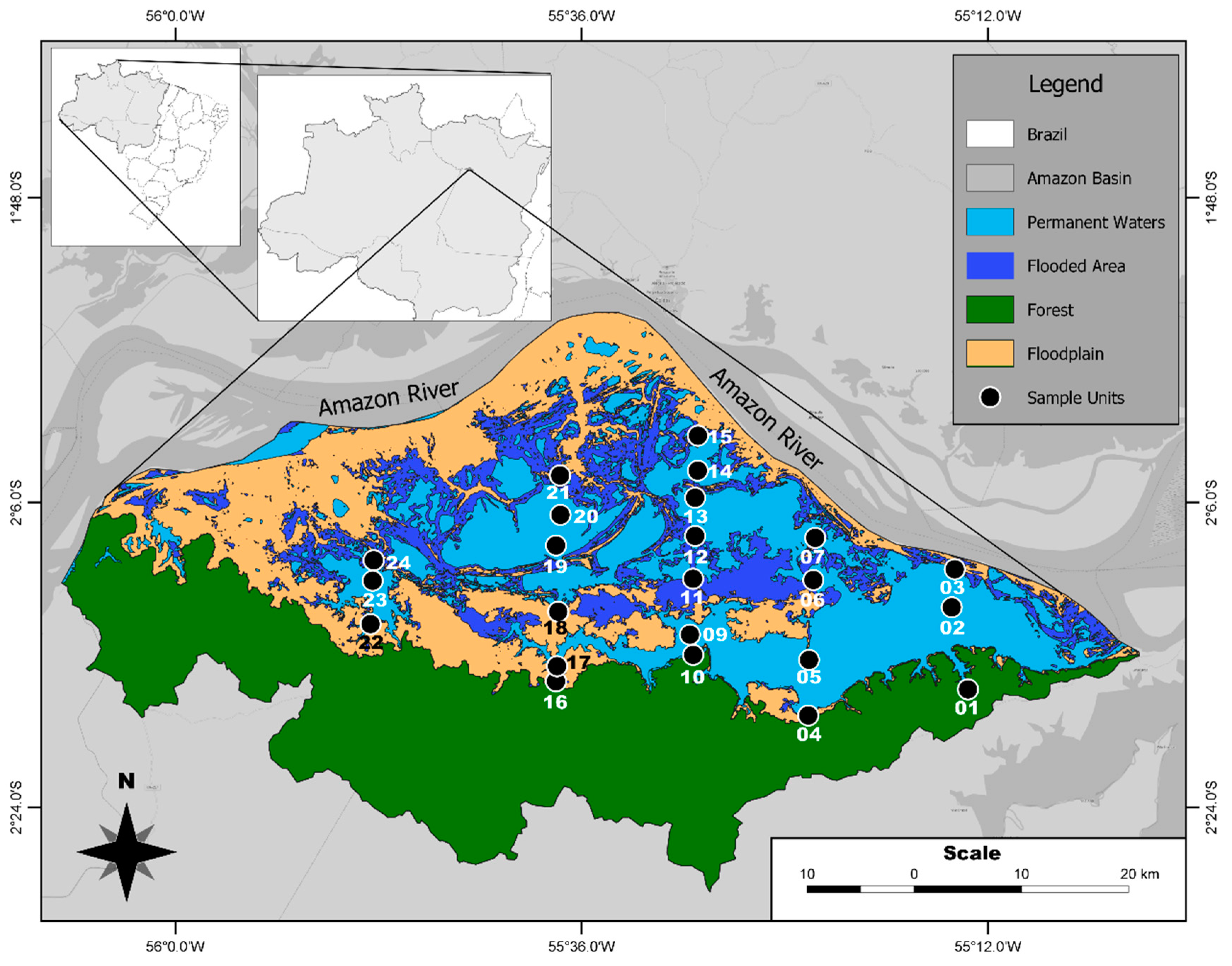
2.1. Environmental and Phytoplankton Data

Sub-surface water samples for nutrients and carbon analyses were collected at the same locations where phytoplankton was collected (Figure 1). Additionally, at these locations, depth (Dep) was recorded and dissolved oxygen (DO), oxygen saturation (O2Sat), and electrical conductivity (Cond) were measured with a multi-parameter probe (YSI 6820-V2). Total phosphorus (TP), orthophosphate (PO4), hydrolyzable reactive phosphorus (HdrP) and organic phosphorus (OP) were quantified following the methods of [51]. Total nitrogen (TN), dissolved nitrogen (DIN), ammonium (NH4), nitrate (NO3) and nitrite (NO2) were analyzed with the non-dispersive infra-red (NDIR). Total organic carbon (TOC), dissolved organic carbon (DOC), particulate organic carbon (POC), total suspended solids (TSS), fixed suspended solids (FSS), and volatile suspended solids (VSS) were measured following procedures in the Standard Methods for the Examination of Water and Wastewater [52].
The quantitative samples of phytoplankton were collected and were stored in 100 mL amber vials and fixed with acetic Lugol solution. Phytoplankton was counted following the Utermöhl method [53], at 400× magnification. The counting was done randomly until obtaining 100 individuals (cells, colonies, or filaments) of the most frequent species, keeping the error less than 20%, with a confidence coefficient of 95% [54]. The adopted system for classifying phytoplankton was that of Guiry and Guiry [55]. The algal biovolume was calculated by multiplying the abundance of each species by the mean cell volume [56], based on the measurement of at least 30 individuals and was expressed in mm3 L−1. This biovolume was used to select the phytoplankton functional groups (FGs). FGs were classified according to Reynolds [29], with the modifications made by Padisák [30]. The FGs’ specific biomass was estimated from the product of the population and mean unit volume and only species that contributed with at least 5% of the total biovolume per sample unit were considered [57].

2.2. Data Analysis

The space-time interaction test (STI) [58] was used to verify how significant the variation in time and in space of the structure of the phytoplankton community was. It is worth mentioning that in our study, time variation is primary linked with hydrology cycling, whereas spatial variation would also be related to processes that have taken place in the different locations of the floodplain. The STI test consisted of a two-way ANOVA to test the space-time interaction, and the main effects of space or time using one among a set of possible models [58]. Firstly, space and time were coded using Helmert contrasts for the main factor effects. Then, they were coded using distance-based Moran Eigenvector Maps variables (dbMEM) for the interaction term. If the interaction was not significant, the test of the main factors was also done following the method for the previous step. If the interaction was significant, then we tested spatial and temporal structures using dbMEM variables to know whether separate spatial or temporal structures exist. For more details consult [58]. These analyses were implemented using the R packages “adespatial”.
To evaluate the importance of nutrients in the structure of the phytoplankton community, we divided the environmental variables into two subgroups, one with the variables related to the nutrients (nitrogen, phosphorus, carbon, and oxygen) and another group with the other variables to which we refer to as hydrological variables. These two groups were used to perform a partial redundancy analysis [59]. This analysis allowed us to estimate the importance and influence of different environmental variables partitions (i.e., nutrients and hydrological) in the structure of the phytoplankton community. To test the significance of each partition we performed an ANOVA test. These analyses were implemented using the R packages “vegan” [60].
We performed an analysis of the organization of three-way tables with Co-Inertia analysis’ (STATICO) to evaluate the relationships between the phytoplankton biomass and nutrients. With this method, we calculated the stable part of the relationships between nutrients and phytoplankton throughout the hydrological periods. STATICO combines two analyses, the STATIS that is finding the stable part of the structure in a series of tables and the co-inertia that consists in finding the common structure in two data tables [61]. The STATICO maximizes the covariance between the row coordinates of two tables. The pair of tables here consist of one for the phytoplankton biomass and one for the nutrient conditions. This analysis had three-steps: (i) Each table was analyzed with a primary analysis; so, (ii) each pair was linked by co-inertia analysis that produces a cross table; then (iii) the partial triadic analysis (PTA) was used to analyze the series of cross tables [62]. We evaluated four pairs of tables: Rising (RS), flushing (FL), high-water (HW) and low-water (LW). With the interstructure, we evaluated the variation of the phytoplankton–nutrients relationship. Hence, it is possible to quantify the strength of the phytoplanknton biomass–nutrients relationship over the hydrological periods. The compromise determines the part of the structure between phytoplankton biomass and the nutrients that remain stable throughout the hydrological periods. These analyses were implemented using the R packages “ade4” [61].
We used a forward selection procedure [63] to keep only the environmental variables that significantly influence the phytoplankton community structure. This procedure consists of a global test using all possible explanatory variables. Then, if, and only if, the global test was significant, one can proceed with the forward selection. The procedure has two stopping criteria, and when a variable that brings one or the other criterion over the fixed threshold is identified, that variable is rejected, and the procedure is stopped. For more details consults [63]. With the selected variables, we performed a Multiple Regression Tree [64] to evaluate if the relationship between phytoplankton and the selected environmental variables were an important factor in structuring the community. The Multiple Regression Tree (MRT) consists of a constrained partitioning of the data parallel cross-validation of the results that produce a model that forms a decision tree [65]. This method forms clusters of sites by repeating splitting of the data along axes of the explanatory variables. Each split was chosen to minimize the dissimilarity of data within the clusters [64,66] that were presented graphically by a tree. The overall fit of the tree was specified as adjusted R2 (adjR2), and the predictive accuracy was assessed by cross-validated relative error (CVRE) [66]. The MRT was implemented using the R packages “mvpart” [67] and “MVPARTwrap” [68]. We also performed an Indicator Species Analysis (Ind-Val) to find a statistically significant phytoplankton functional group for each data split and groups resulting from MRT [69]. The method combines FG mean abundance (“specificity”) and frequency of occurrence (“fidelity”). FGs that are both abundant and occur in most of the hydrological periods, belonging to one MRT group have a high Ind-Val. Ind-Val ranges between 0 to 1, where 1 refers to a perfect indicator regarding both “specificity” and “fidelity.” We applied the Ind-Val to groups obtained with the MRT analysis using the R package “MVPARTwrap”.

3. Results

3.1. Hydrological and Nutrients Data

Depth, conductivity, and suspended solids presented contrasted mean values in function of the hydrological periods (Table 1). Depth was comparable between FL and RS, it was three time higher during HW than during LW. Conductivity was comparable between FL and LW periods but was 60% higher during FL than during HW. Suspended solids (TSS and FSS) were minimum during HW and maximum during LW.
The total nitrogen mean value (TN) was maximum during LW, about one third greater than during FL when it was minimum. On the other hand, if total inorganic nitrogen (DIN) was also maximum during LW, it was minimum during the RS. The main form of inorganic nitrogen was NO3 except during LW when NH4 was more than half DIN. NO2 remained low below 10 µg L−1 except during LW when it reached up to 80 µg L−1, while NO3 is very low. Total organic carbon (TOC) was maximum during RS and minimum during LW with a mean value ranging between 4 and 5.5 mg L−1. The dissolved fraction (DOC) represented up to 93% of TOC during FL and 65% during RS. During the rising and flushing periods, PO4 only represents a small part of total phosphorus, respectively 6% and 2%. During the high- and low-water periods, it represents 40% and 78% respectively. The water column remained oxygenated with saturation above 58% regardless of the hydrological period.

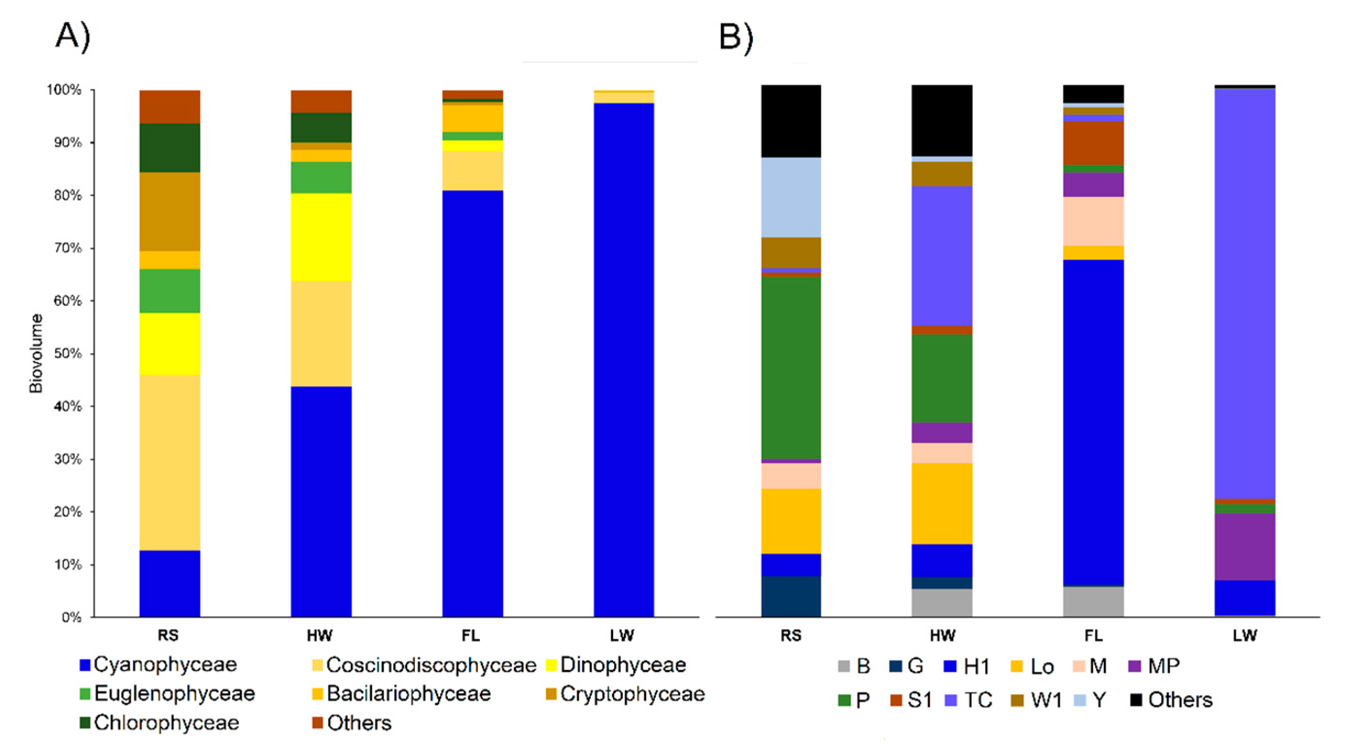
3.2. Biological Data

The proportion of classes in the composition of the phytoplankton community varies throughout hydrological periods (Figure 2A). The Coscinodiscophyceae phytoplankton class had the highest biovolume during RS, the representative species was Aulacoseira spp. The Cyanophyceae phytoplankton class presented the highest biovolume during HW, FL and LW periods. The species with the highest biovolume during HW were Phormidium spp and Aulacoseira granulata var granulata. The species that were representative during the FL also presented the highest biovolume in this period were Dolichospermum spp and Gleiterinema splendidum. During LW, the species Oscilatoria spp and Phormidium spp presented the highest biovolume. Interestingly, the proportion of Cyanophyceae increased along the hydrological cycle from RS to LW when the phytoplankton is almost entirely composed (up to 98%) of representatives from this class. Species were distributed in 11 functional groups that contributed to at least 5% of the total biovolume in at least one of the hydrological periods (Figure 2B). During RS, the functional groups P, Y, and Lo comprised 61.4% of the total biovolume. The group P is composed of species adapted to shallow lakes that tolerate high trophic states such Aulacoseira granulata, Closterium sp, and Fragilaria sp. The group Y comprises species adapted to lentic ecosystems and in the study was represented by Cryptomonas spp. The group Lo contains species adapted to deep and shallow lakes that tolerate oligo to eutrophic states such Peridinium spp, and Merismopedia spp. During HW, functional groups were Tc, P, and Lo that represented 58.2% of the total biovolume. The group Tc encompasses species adapted to eutrophic standing waters, or slow-flowing rivers and was here composed by Oscilatoria spp and Phormidium spp. During FL, the group H1 represented 61.1% of the total biovolume. The group H1 comprises species adapted to shallow lakes with eutrophic state and low nitrogen content and was here composed by Dolichospermum spp that may have the ability to fix nitrogen. During LW, the group Tc represented 77.0% of total biovolume, and Oscilatoria spp comprised about 90% of this total. This group encompasses species adapted to eutrophic standing waters, or slow flowing rivers and was here composed by epiphytic cyanobacteria as Oscillatoria spp and Phormidium spp.

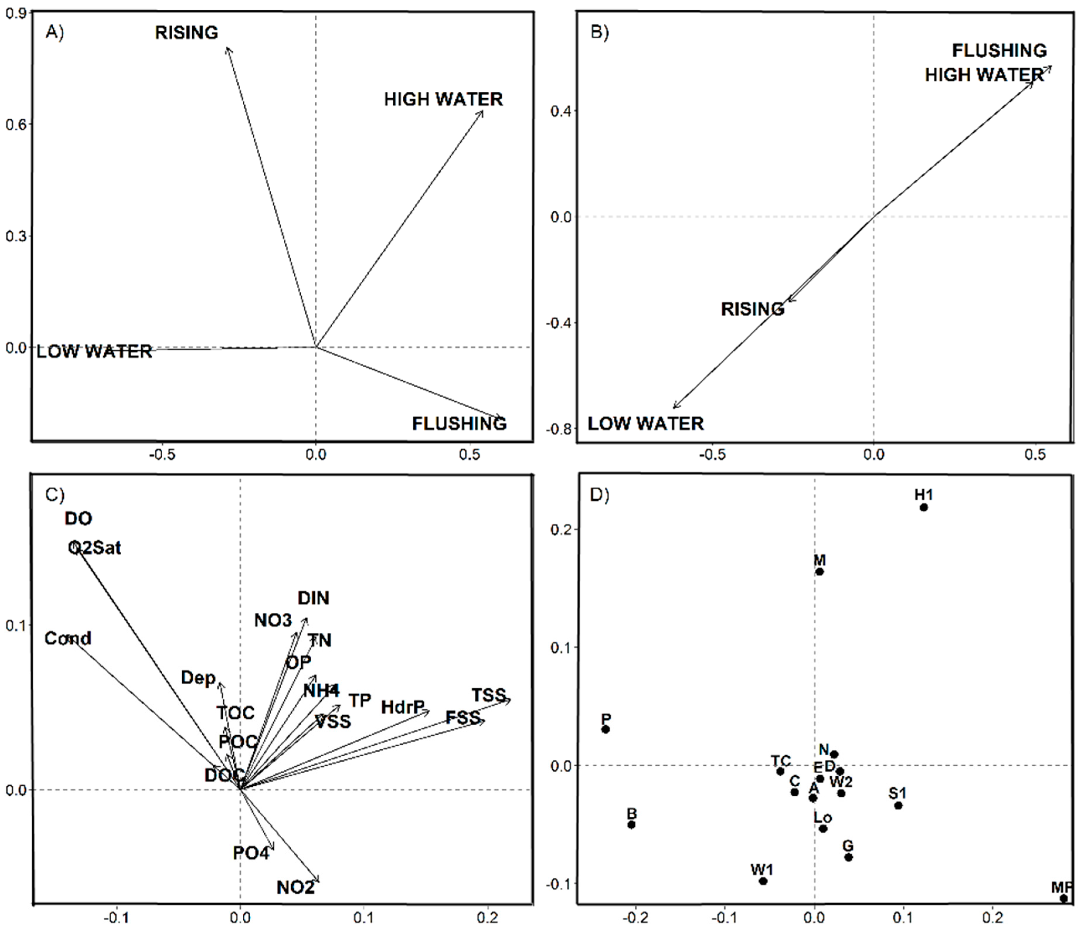
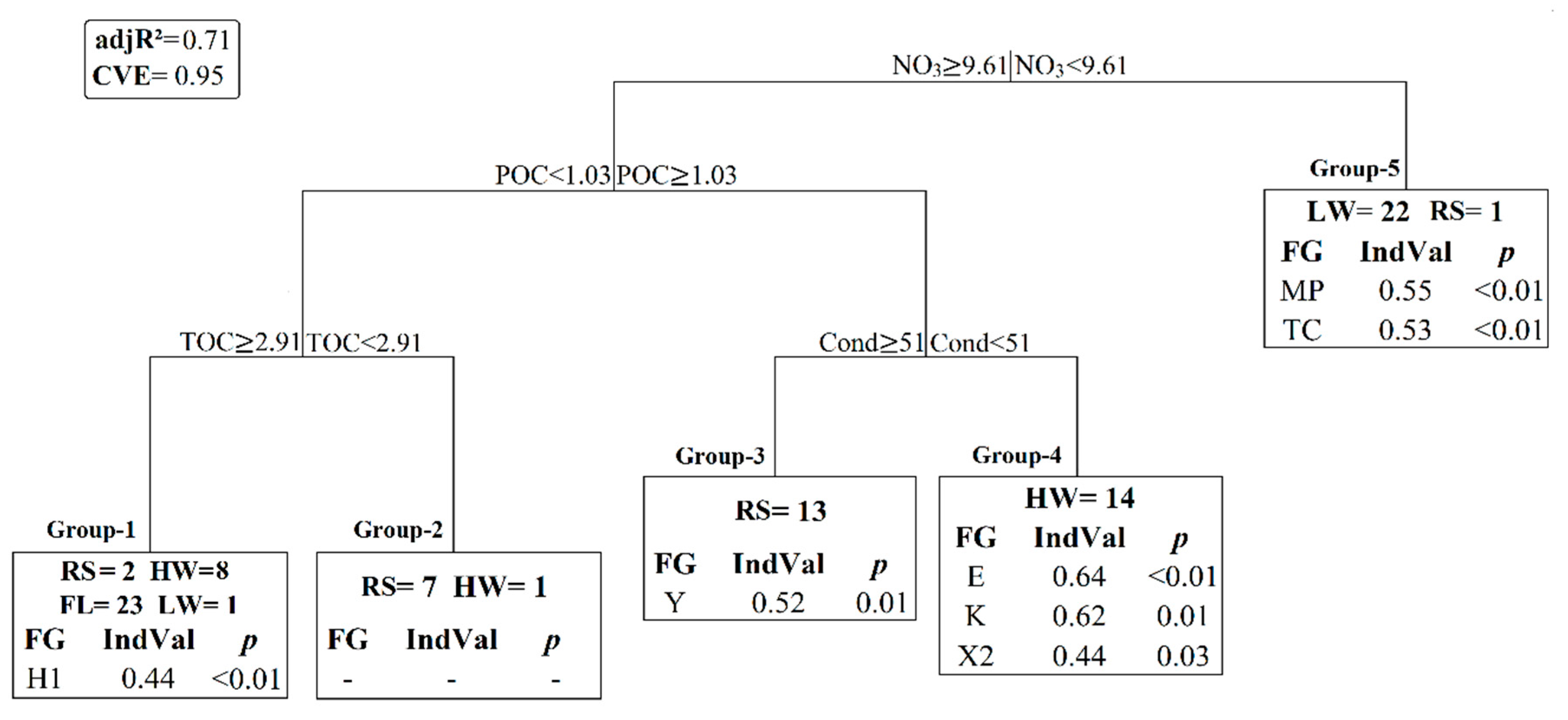
3.3. Statistical Results

The STI test indicated that the space-time interaction is not significant. That is there was no significant influence of space-time on the structuring of the phytoplankton community at the functional group level. The second step returned that only time had a significant importance in structuring the phytoplankton community, hence indicating that spatial distribution of sample units had no significant influence (Table 2). The time influence indicates that the hydrological cycle was the main factor in the dynamics of the phytoplankton community. The partial redundancy analysis (pRDA) for partition environmental data shows that both, nutrients and hydrological variables, had a significant influence in structuring the phytoplankton community, but the strength of the nutrients partition was higher than that of hydrological variables (Table 2). The pRDA also returns a great residual, indicating that there were other important factors, not measured, which influenced the phytoplankton community structure.
The STATICO analysis showed stability in the phytoplankton–nutrient relationship along periods as illustrated by the longer arrows in the interstructure graph (Figure 3A). In these graphs, the greater length of arrows (or in case of points, the distance from the center), the higher the stability in this relationship. However, the weight of each hydrological period on the phytoplankton–nutrients relationship was different (Figure 3B). The first and second axes represented, respectively, 19% and 10% of the total variability. The first axis (horizontal axis) in the compromise graph (Figure 3C) accounted for 42% of the explained variance and the second axis (vertical axis) accounted for 20% of the explained variance and was less significant. Flushing and low-water periods were more related to the first axis which has twice the explanatory power of the second axis. Hence, the phytoplankton–nutrients relationship might be considered stronger during these two periods.
As shown by the environmental variables compromise plot (Figure 3C), the first axis (horizontal), was more related to hydrolyzable phosphorus and suspended solids. The second axis (vertical) was more related with PO4 and NO2 (Figure 3C). Other variables such as conductivity and oxygen, are related to both axes and also have a great compromise (long arrow). The environmental variables with shorter arrows have weak stability with the hydrological cycle and are more related to a specific period, as detailed below. For the functional groups compromise plot (Figure 3D), the most important groups are those more distant to the center of the graph. The FG’s MP and H1 although have great stability with the hydrological cycle, also play an important role on specific period (Figure 4).
MRT applied to the data resulted in five groups, the model explained 71% of the phytoplankton data variability (adjR2 = 0.71). The predictive power of the model expressed as the cross-validation relative error (CVRE) was 0.95. MRT clearly separated LW samples (22 samples) apart from those collected during the other periods based on NO3 concentration (Figure 4); LW samples belonged to group 5 with low NO3 concentration. Further group divisions were based successively upon particulate organic carbon, total organic carbon and conductivity. Interestingly, similarly as LW period, all samples from the FL period are gathered into a single group (group 1) characterized by high NO3, POC and TOC concentrations, whereas samples collected during HW or RS are spread over three groups. A majority of samples collected in HW were gathered into group 4 (high NO3, high POC and low Cond), and those collected during RS mostly divided into two groups, a majority in group 3 (high NO3, high POC, high Cond). Indicator value (Ind-Val), coupled with MRT analysis, enabled extracting sets of FG’s indicators of the MRT groups (Figure 4). Based on the Ind-Val, four groups are characterized by seven significant FGs (p < 0.05). Group 2 does not have any FG indicators with a significative value.

4. Discussion

4.1. Space-Time Components and Environmental Partitions

As we expected, the hydrological variation (time), is a more significant factor of structuration of the functional phytoplankton community than the environmental spatial variability (space). Besides the STI test, the STATICO also showed that most of the phytoplankton community variation is strongly linked with variables related with hydrological conditions (TSS, Cond). MRT further confirmed the groups according to the hydrological periods. The analyses show that only the hydrological variation is strong enough to produce functional changes in the phytoplankton community and this reflects the importance of flood pulse dynamics in the Amazon basin. In fact, the hydrological variation or flood pulse, is acknowledged as a strength that can promote changes in these environments and biological communities in several studies [36,70,71]. In addition, our results showed that these changes are more related to nutrients changes (and especially nitrogen changes as indicated by MRT) than changes in another factors (among those we have measured). Indeed, the partition test showed that although the hydrological variables measured were significant in structuring the community, the nutrients variables were two times more decisive in this process, thus confirming our starting hypothesis. In addition, the partition involving both variables (Hydr + Nutr) has the same proportion than that of the nutrients partition. The hydrological annual variability promotes a lot of changes over the year, and one of them is a variability of the different kinds of nutrients. In general, we measured only total nitrogen and total phosphorus when performing research in this field, for many reasons, but the different fractions of nitrogen and phosphorus compounds have different influences on the phytoplankton community.

4.2. Nutrients-Phytoplankton Relationships over Hydrological Cycle

Our results showed that over the hydrological year, (i) the interaction between phytoplankton community and phosphorus compounds is more stable than that of nitrogen compounds (Figure 3C,D), and (ii) that the rising period has the weakest weight in the phytoplankton–nutrients interaction (Figure 3B). While the phytoplankton biovolume becomes higher, the weight of the relationship in subsequent hydrological periods increases, suggesting that there are both top-down and bottom-up controls, for the phosphorus and nitrogen cycles in tropical floodplain system. Top-down refers to the input which occurs in the rising period from waters coming from the Amazon river, while bottom-up refers to phosphorus (or nitrogen) cycle processes occurring inside the floodplain.
Regarding phosphorus, our results suggest that bottom-up control is stronger than top-down, or in other words, that phosphorus compounds already present or in situ recycled in the system have a greater influence upon phytoplankton than allogenic phosphorus compounds. It is well known that Amazonian rivers that drain the Andes (classified as white-water rivers according to Sioli, 1984 typology) [47] carry high concentration in suspended solids and dissolved and sediment-bound nutrients [37]. The river incursion across the floodplain during rising brings nutrients and sediment into the floodplain ecosystems and promotes a high peak in primary productivity [39,72]. However, our results also showed that the phytoplankton–phosphorus relationship is stable along the hydrological year. Many processes can participate to maintain a rather constant concentration of phosphorus in the water column: Seasonal herbaceous plants that pump nutrients from the sediment to support their growth and release nutrients in the water column during their decay [73,74]; sediment early diagenesis processes and resuspension may also participate [74].
Although weaker than with phosphorus compounds, our results showed that there is a stable interaction between nitrogen compounds (TN and DIN) and phytoplankton. Wetlands such as floodplains can be considered aggrading ecosystems where the nitrogen can come from adjacent drained areas or the mainstream, and in some cases, from biological nitrogen fixation and atmospheric deposition [75,76,77]. The phytoplankton primary productivity peak occurring in the rising period is followed by a significant increase of nitrogen-fixing cyanobacteria biovolume. Nitrogen fixation is an essential process for eutrophic wetlands, once it may contribute from 5% to 80% of the total nitrogen inputs in these systems [8]. NO3 is the most common reactive nitrogen species [74], and the high concentration in flushing period allied to higher biovolume of FG H1 suggest that nitrogen-fixing process plays an essential role in maintaining the stability along the hydrological cycle.
Besides nitrogen-fixation processes, the increases in nitrogen compounds between rising and subsequent periods, similar to phosphorus, can be influenced by processes mentioned above, especially the seasonal herbaceous plants growth/decay cycle that may release NH4 and NO3 in the water column. Thus, the sediment nutrients pool mobilization is another crucial factor that permits the nitrogen concentration to remain stable during the hydrological cycle. Hence, like phosphorus, the phytoplankton–nitrogen interaction also suggests that there is both a top-down and bottom-up interaction for its cycle in tropical floodplain system.
The idea that the phytoplankton has the potential to influence pools of nitrogen and phosphorus that would be available is not new [77], but works with this approach are scarce in tropical environments. For temperate lakes, the work of Cottingham et al. [77], has demonstrated that cyanobacteria have the potential to drive nitrogen and phosphorus cycles in lakes. They remarked that the ability of many cyanobacterial taxa to fix nitrogen and to access pools of phosphorus in sediments and bottom waters is the key behind this influence. Their work suggests that cyanobacterial blooms warrant attention as potential drivers of the transition from a low-nutrient clear-water regime to a high-nutrient turbid-water regime. Our results show that there is a considerable increase in cyanobacteria biovolume, but it is difficult to know how much is a consequence of allochthonous nitrogen inputs and how much is a consequence of autochthonous nitrogen inputs. However, it is certain that this increase is an important factor for maintaining the stability of nutrients over the hydrological cycle. Thus, the cyanobacteria dynamics are an essential factor in both nutrients cycling and phytoplankton dynamics. Increases in nutrients leading to a dominance of cyanobacteria have been reported by Dokulil and Teubner [78], and in Curuai, Affonso et al. [79] they found that the flushing period was the most eutrophic period. Thus, the extent to which the floodplain becomes shallow, and water flow less intense, the cyanobacteria community can be established [80].

4.3. Cyanobacteria Dynamics

The results showed that while the phytoplankton biomass increased, and the environment became more eutrophic, the phytoplankton functional group diversity was decreasing until the phytoplankton was almost entirely composed by the cyanobacteria group. Even if phytoplankton species differ in their nutritional requirements [81], and although nitrogen and phosphorus are essential factors for the phytoplankton growth, they are not the unique. Other factors play a vital role for the phytoplankton in specific periods. Unlike during the flushing and low-water periods, samples collected during the rising and high-water periods spread over a larger number of MRT groups with functional groups with significant Ind-Val. The Amazon river incursion extent across the floodplain, the flow magnitude and the mixture of this inflow with the water residing on the floodplain cause a significant directional gradient [82]. Additinoally, the rising period is probably the period that is the most influenced by the floodplain geomorphology. The FG Y has a significant value of Ind-Val for 13 sites in rising period and it is an indication that this period is marked by a great dynamism. Indeed, the group Y refers to a wide range of habitats, thus reflecting the ability of species to live in almost all lentic ecosystems [30]. During the high-water period, a majority of the samples were gathered into a group that exhibited three functional groups with significant Ind-Val. These results are an indication of heterogeneity and of a state of a transition period.
The reduction of water speed and input of nutrients from the previous periods turns the environment favorable to cyanobacteria community development. High NO3 concentration with lower concentrations of POC and higher concentrations of TOC characterize all sites in the flushing period. NO3 and NH4 are the preferred uptake forms of nitrogen by phytoplankton, but NH4 might have an inhibitory or repressive effect in NO3 uptake and assimilation [10]. During the flushing period NH4 is very low, while NO3 is high: A condition that favors the NO3 uptake by the phytoplankton during this period. During this period also, POC was very low and TOC was almost entirely in DOC form. As mentioned in Moreira-Turc et al. [42], contrasting with the rising period when DOC is mainly imported from the Amazon River, high DOC lability is expected during the flushing period because it is mainly originating from phytoplankton production. Higher labile DOC concentration also helps to provide nutrients for the development and establishment of the cyanobacteria community [16,17,18]. Lowest concentrations of NH4 also favor the increase of nitrogen-fixing cyanobacteria and our results show that functional group H1, composed of species with nitrogen-fixing ability, has a significative Ind-Val for samples collected during the flushing period. NO3 depletion characterized almost all the samples collected during the low-water period, while NO2 increased. Due to lowest water level and increasing interaction between water column and sediment, denitrification bacteria in the sediment (that might have anoxia or hypoxia condition), can be responsible for the characteristics of the low-water period. Even though the low-water period was composed almost entirely by one functional group, the Ind-Val comprised two groups with significant indicator-values, composed of species adapted to eutrophic waters and shallow turbid lakes with the presence of inorganic compounds. These results demonstrate that despite the dominance of cyanobacteria, the conditions begin to be favorable for the establishment of other phytoplankton groups that will encounter favorable conditions during the next hydrological cycle.

5. Conclusions

Our analyses confirm the predominant role of hydrology upon the phytoplankton community. The seasonal hydrological variation is strong enough to produce functional changes in phytoplankton community, especially because the changes in nitrogen and phosphorus contents and chemical speciation along the water year. Besides, biogeochemical processes in tropical floodplain lakes, such as the Curuai floodplain lake, enable maintaining phytoplankton nutrient requirements even long after the nutrient inputs from the river water has declined. The nutrient inputs in rising periods increases the phytoplankton biomass which becomes dominated by cyanobacteria during the low-water period. The cyanobacteria, allied to other organisms (not evaluated in this study such as macrophytes and bacteria), play an important role in maintaining the stability of nutrients along hydrological periods. Interestingly, it was possible to identify a limited number of phytoplankton functional groups indicating the particular environmental conditions during the flushing and low-water periods. During the rising and high-water periods, the environmental and biological conditions seem to be more spatially structured in part because of higher water contribution from the local watershed at these periods. These features highlight the large variability in phytoplankton activities in tropical floodplain ecosystems that may cause issues for the global Amazonian trophic chain. Although our study contributes disentangling hydrology and nutrients control upon the phytoplankton community and better understands how the nutrients–phytoplankton relationship changes along the water year, still more research is required upon the phytoplankton–nutrient relationship in tropical aquatic ecosystems. Most of the knowledge upon this relationship is based on experimental investigations and research in temperate environments, and thus limiting our understanding of what controls such processes in tropical freshwater ecosystems.

Author Contributions

C.N.K. and M.-P.B. were mainly responsible for the development and organization of the work. I.d.S.N. and M.T.M.P.S.L. assisted in the taxonomic identification of the phytoplankton community and in the ecological interpretation of community results. D.d.M.M. contributed to the analytical procedure of water and the ecological interpretation of the data obtained. J.G. assisted with the geochemical assessment. L.C.G.V. assisted in the development and analysis of statistical data applied to the ecological community.

Funding

The authors are very grateful to the two anonymous revisors, their constructive comments helped to substancially improve the manuscript. This research was done under the auspices of CNPq (Conselho Nacional de Desenvolvimento Científico e Tecnológico, Brazil), CAPES (Coordenação de Aperfeiçoamento de Pessoal de Nível Superior, Brazil), IRD (Institut de Recherche pour le Développement, grant number 490634/2013-3, France) and LMI OCE (Laboratoire Mixte International ‘Observatoire des Changements Environnementaux’) and of three research programs, Clim-FABIAM, which was funded by FRB (Fondation pour la Recherche sur la Biodiversité) and Bloom-ALERT, which was funded by the GUYAMAZON program (IRD/CIRAD/Ambassade de France/FAPEAM), and INCT nº 16- 2014 ODISSEIA, with funding from CNPq/CAPES/FAP-DF The paper also received funding from the European Union’s Horizon 2020 Research and innovation program under the Marie Skłodowska—Curie grant agreement Nº 691053.

Conflicts of Interest

The authors declare no conflict of interest.

References

  1. Fiore, M.D.F.; Neilan, B.A.; Copp, J.N.; Rodrigues, J.L.M.M.; Tsai, S.M.; Lee, H.; Trevors, J.T. Characterization of nitrogen-fixing cyanobacteria in the Brazilian Amazon floodplain. Water Res. 2005, 39, 5017–5026. [Google Scholar] [CrossRef] [PubMed]
  2. Schindler, D.W. The dilemma of controlling cultural eutrophication of lakes. Proc. R. Soc. B Biol. Sci. 2012, 279, 4322–4333. [Google Scholar] [CrossRef] [PubMed] [Green Version]
  3. Paerl, H.W.; Gardner, W.S.; Havens, K.E.; Joyner, A.R.; McCarthy, M.J.; Newell, S.E.; Qin, B.; Scott, J.T. Mitigating cyanobacterial harmful algal blooms in aquatic ecosystems impacted by climate change and anthropogenic nutrients. Harmful Algae 2016, 54, 213–222. [Google Scholar] [CrossRef] [PubMed] [Green Version]
  4. Thomas, M.K.; Litchman, E. Effects of temperature and nitrogen availability on the growth of invasive and native cyanobacteria. Hydrobiologia 2016, 763, 357–369. [Google Scholar] [CrossRef]
  5. Schindler, D.W.; Hecky, R.E.; Findlay, D.L.; Stainton, M.P.; Parker, B.R.; Paterson, M.J.; Beaty, K.G.; Lyng, M.; Kasian, S.E.M. Eutrophication of lakes cannot be controlled by reducing nitrogen input: Results of a 37-year whole-ecosystem experiment. Proc. Natl. Acad. Sci. USA 2008, 105, 11254–11258. [Google Scholar] [CrossRef] [PubMed] [Green Version]
  6. Conley, D.J.; Paerl, H.W.; Howarth, R.W.; Boesch, D.F.; Seitzinger, S.P.; Havens, K.E.; Lancelot, C.; Likens, G.E. Controlling Eutrophication: Nitrogen and Phosphorus. Science 2009. [Google Scholar] [CrossRef]
  7. Howarth, R.W. Nutrient Limitation of Net Primary Production in Marine Ecosystems. Annu. Rev. Ecol. Syst. 1988, 19, 89–110. [Google Scholar] [CrossRef]
  8. Lewis, W.M.; Wurtsbaugh, W.A.; Paerl, H.W. Rationale for Control of Anthropogenic Nitrogen and Phosphorus to Reduce Eutrophication of Inland Waters. Environ. Sci. Technol. 2011, 45, 10300–10305. [Google Scholar] [CrossRef] [PubMed]
  9. Elser, J.J.; Bracken, M.E.S.; Cleland, E.E.; Gruner, D.S.; Harpole, W.S.; Hillebrand, H.; Ngai, J.T.; Seabloom, E.W.; Shurin, J.B.; Smith, J.E. Global analysis of nitrogen and phosphorus limitation of primary producers in freshwater, marine and terrestrial ecosystems. Ecol. Lett. 2007, 10, 1135–1142. [Google Scholar] [CrossRef] [Green Version]
  10. Abell, J.M.; Özkundakci, D.; Hamilton, D.P. Nitrogen and Phosphorus Limitation of Phytoplankton Growth in New Zealand Lakes: Implications for Eutrophication Control. Ecosystems 2010, 13, 966–977. [Google Scholar] [CrossRef] [Green Version]
  11. Thad Scott, J.; McCarthys, M.J. Nitrogen fixation may not balance the nitrogen pool in lakes over timescales relevant to eutrophication management. Limnol. Oceanogr. 2010, 55, 1265–1270. [Google Scholar] [CrossRef] [Green Version]
  12. Scheffer, M.; Van Nes, E.H. Shallow lakes theory revisited: Various alternative regimes driven by climate, nutrients, depth and lake size. Hydrobiologia 2007, 584, 455–466. [Google Scholar] [CrossRef]
  13. Janssen, A.B.G.; Teurlincx, S.; An, S.; Janse, J.H.; Paerl, H.W.; Mooij, W.M. Alternative stable states in large shallow lakes? J. Great Lakes Res. 2014, 40, 813–826. [Google Scholar] [CrossRef] [Green Version]
  14. Jeppesen, E.; Meerhoff, M.; Davidson, T.A.; Trolle, D.; Søndergaard, M.; Lauridsen, T.L.; Beklioglu, M.; Brucet, S.; Volta, P.; González-Bergonzoni, I.; et al. Climate change impacts on lakes: An integrated ecological perspective based on a multi-faceted approach, with special focus on shallow lakes. J. Limnol. 2014, 73, 88–111. [Google Scholar] [CrossRef]
  15. Lobo, M.T.M.P.S.; de Souza Nogueira, I.; Fabris Sgarbi, L.; Nunes Kraus, C.; de Oliveira Bomfim, E.; Garnier, J.; da Motta Marques, D.; Bonnet, M.-P. Morphology-based functional groups as the best tool to characterize shallow lake-dwelling phytoplankton on an Amazonian floodplain. Ecol. Indic. 2018, 95, 579–588. [Google Scholar] [CrossRef]
  16. Lampert, W.; Sommer, U. Limnoecology; Oxford University Press: Oxford, UK, 2007; ISBN 978-0-19-921392-4. [Google Scholar]
  17. Søndergaard, M.; Jensen, J.P.; Jeppesen, E. Role of sediment and internal loading of phosphorus in shallow lakes. Hydrobiologia 2003, 506–509, 135–145. [Google Scholar]
  18. Scheffer, M.; Rinaldi, S.; Gragnani, A.; Mur, L.R.; van Nes, E.H. On the Dominance of Filamentous Cyanobacteria in Shallow, Turbid Lakes. Ecology 1997, 78, 272. [Google Scholar] [CrossRef]
  19. Hays, S.G.; Ducat, D.C. Engineering cyanobacteria as photosynthetic feedstock factories. Photosynth. Res. 2014, 123, 1–11. [Google Scholar] [CrossRef]
  20. Benoiston, A.-S.; Ibarbalz, F.M.; Bittner, L.; Guidi, L.; Jahn, O.; Dutkiewicz, S.; Bowler, C. The evolution of diatoms and their biogeochemical functions. Philos. Trans. R. Soc. B Biol. Sci. 2017, 372, 20160397. [Google Scholar] [CrossRef]
  21. Peace, A. Effects of light, nutrients, and food chain length on trophic efficiencies in simple stoichiometric aquatic food chain models. Ecol. Model. 2015, 312, 125–135. [Google Scholar] [CrossRef]
  22. O’Neil, J.M.; Davis, T.W.; Burford, M.A.; Gobler, C.J. The rise of harmful cyanobacteria blooms: The potential roles of eutrophication and climate change. Harmful Algae 2012, 14, 313–334. [Google Scholar] [CrossRef]
  23. Catherine, Q.; Susanna, W.; Isidora, E.S.; Mark, H.; Aurélie, V.; Jean-François, H. A review of current knowledge on toxic benthic freshwater cyanobacteria—Ecology, toxin production and risk management. Water Res. 2013, 47, 5464–5479. [Google Scholar] [CrossRef]
  24. Boopathi, T.; Ki, J.-S. Impact of Environmental Factors on the Regulation of Cyanotoxin Production. Toxins 2014, 6, 1951–1978. [Google Scholar] [CrossRef] [PubMed] [Green Version]
  25. Rastogi, R.P.; Madamwar, D.; Incharoensakdi, A. Bloom dynamics of cyanobacteria and their toxins: Environmental health impacts and mitigation strategies. Front. Microbiol. 2015, 6, 1–22. [Google Scholar] [CrossRef] [PubMed]
  26. Sukenik, A.; Quesada, A.; Salmaso, N. Global expansion of toxic and non-toxic cyanobacteria: Effect on ecosystem functioning. Biodivers. Conserv. 2015, 24, 889–908. [Google Scholar] [CrossRef]
  27. Vilmi, A.; Karjalainen, S.M.; Landeiro, V.L.; Heino, J. Freshwater diatoms as environmental indicators: Evaluating the effects of eutrophication using species morphology and biological indices. Environ. Monit. Assess. 2015, 187, 243. [Google Scholar] [CrossRef]
  28. Dolman, A.M.; Rücker, J.; Pick, F.R.; Fastner, J.; Rohrlack, T.; Mischke, U.; Wiedner, C. Cyanobacteria and cyanotoxins: The influence of nitrogen versus phosphorus. PLoS ONE 2012, 7, e38757. [Google Scholar] [CrossRef]
  29. LONGHI, M.L.; BEISNER, B.E. Patterns in taxonomic and functional diversity of lake phytoplankton. Freshw. Biol. 2010, 55, 1349–1366. [Google Scholar] [CrossRef]
  30. Colina, M.; Calliari, D.; Carballo, C.; Kruk, C. A trait-based approach to summarize zooplankton–phytoplankton interactions in freshwaters. Hydrobiologia 2015, 767, 221–233. [Google Scholar] [CrossRef]
  31. Salmaso, N.; Naselli-Flores, L.; Padisák, J. Functional classifications and their application in phytoplankton ecology. Freshw. Biol. 2015, 60, 603–619. [Google Scholar] [CrossRef]
  32. Reynolds, C.S.; Huszar, V.; Kruk, C.; Naselli-Flores, L.; Melo, S.S. Towards a functional classification of the freshwater phytoplankton. J. Plankton Res. 2002, 24, 417–428. [Google Scholar] [CrossRef] [Green Version]
  33. Padisák, J.; Crossetti, L.O.; Naselli-Flores, L. Use and misuse in the application of the phytoplankton functional classification: A critical review with updates. Hydrobiologia 2009, 621, 1–19. [Google Scholar] [CrossRef]
  34. Kruk, C.; Huszar, V.L.M.; Peeters, E.T.H.M.; Bonilla, S.; Costa, L.; Lürling, M.; Reynolds, C.S.; Scheffer, M. A morphological classification capturing functional variation in phytoplankton. Freshw. Biol. 2010, 55, 614–627. [Google Scholar] [CrossRef]
  35. Machado, K.B.; Borges, P.P.; Carneiro, F.M.; de Santana, J.F.; Vieira, L.C.G.; de Moraes Huszar, V.L.; Nabout, J.C. Using lower taxonomic resolution and ecological approaches as a surrogate for plankton species. Hydrobiologia 2015, 743, 255–267. [Google Scholar] [CrossRef]
  36. Junk, W.J.; Bayley, P.B.; Sparks, R.E. The flood pulse concept in river-floodplain systems. Can. Spec. Publ. Fish. Aquat. Sci. 1989, 106, 110–127. [Google Scholar]
  37. Junk, W.J.; Piedade, M.T.F.; Schöngart, J.; Wittmann, F. A classification of major natural habitats of Amazonian white-water river floodplains (várzeas). Wetl. Ecol. Manag. 2012, 20, 461–475. [Google Scholar] [CrossRef]
  38. Tockner, K.; Malard, F.; Ward, J.V. An extension of the flood pulse concept. Hydrol. Process. 2000, 14, 2861–2883. [Google Scholar] [CrossRef]
  39. Bonnet, M.P.P.; Barroux, G.; Martinez, J.M.M.; Seyler, F.; Moreira-Turcq, P.; Cochonneau, G.; Melack, J.M.M.; Boaventura, G.; Maurice-Bourgoin, L.; León, J.G.G.; et al. Floodplain hydrology in an Amazon floodplain lake (Lago Grande de Curuaí). J. Hydrol. 2008, 349, 18–30. [Google Scholar] [CrossRef] [Green Version]
  40. Junk, W.J.; Wantzen, K.M. The flood pulse concept: New aspects, approaches and applications—An update. In Proceedings of the Second International Symposium on the Management of Large Rivers for Fisheries, Rome, Italy, 11–14 February 2003; pp. 117–149. [Google Scholar]
  41. Bonnet, M.-P.; Pinel, S.; Garnier, J.; Bois, J.; Resende Boaventura, G.; Seyler, P.; Motta Marques, D. Amazonian floodplain water balance based on modelling and analyses of hydrologic and electrical conductivity data. Hydrol. Process. 2017, 31, 1702–1718. [Google Scholar] [CrossRef]
  42. Kraus, C.N.; Bonnet, M.P.; Miranda, C.A.; de Souza Nogueira, I.; Garnier, J.; Vieira, L.C.G. Interannual Hydrological Variation and Ecological Phytoplankton Patterns in Amazonian Floodplain Lakes. Hydrobiologia 2018. [Google Scholar] [CrossRef]
  43. Sioli, H. The Amazon and its main affluents: Hydrography, morphology of the river courses, and river types. In The Amazon: Limnology and Landscape Ecology of a Mighty Tropical River and Its Basin; Sioli, H., Ed.; Springer: Dordrecht, The Netherlands, 1984; pp. 127–165. ISBN 978-94-009-6542-3. [Google Scholar]
  44. Moquet, J.S.; Crave, A.; Viers, J.; Seyler, P.; Armijos, E.; Bourrel, L.; Chavarri, E.; Lagane, C.; Laraque, A.; Casimiro, W.S.L.; et al. Chemical weathering and atmospheric/soil CO(2) uptake in the Andean and Foreland Amazon basins. Chem. Geol. 2011, 287, 1–26. [Google Scholar] [CrossRef]
  45. Park, E.; Latrubesse, E.M. Water resources research. Water Resour. Res. 2015, 51, 9127–9140. [Google Scholar]
  46. Bonnet, M.P.; Garnier, J.; Barroux, G.; Boaventura, G.R.; Seyler, P.; Mse, C.C.; Bataillon, P.E. Biogeochemical functioning of amazonian floodplains: The case of lago Grande de Curuai. In Riparian Zones: Characteristics, Management Practices and Ecological Impacts, Environmental Research Advances; Pokrovsky, O.S., Viers, J., Eds.; Nova Science Publishers: New York, NY, USA, 2016; pp. 1–22. ISBN 978-1-63484-636-3. [Google Scholar]
  47. APHA Standard Methods for Examination of Water and Wastewater (Standard Methods for the Examination of Water and Wastewater); Standard Methods; American Public Health Association (APHA): Washington, DC, USA, 1998; pp. 5–16.
  48. Utermöhl, H. Zur vervollkommnung der quantitativen phytoplankton-methodik. Mitt. Int. Ver. Angew. Limnol. 1958, 9, 1–38. [Google Scholar] [CrossRef]
  49. Lund, J.W.G.; Kipling, C.; Le Cren, E.D. The inverted microscope method of estimating algal numbers and the statistical basis of estimations by counting. Hydrobiologia 1958, 11, 143–170. [Google Scholar] [CrossRef]
  50. Guiry, M.D.; Guiry, G.M. AlgaeBase. World-Wide Electronic Publication. Available online: http//www.algaebase.org (accessed on 20 October 2018).
  51. Hillebrand, H.; Dürselen, C.-D.; Kirschtel, D.; Pollingher, U.; Zohary, T. Biovolume Calculation for Pelagic and Benthic Microalgae. J. Phycol. 1999, 35, 403–424. [Google Scholar] [CrossRef]
  52. Kruk, C.; Mazzeo, N.; Lacerot, G.; Reynolds, C.S. Classification schemes for phytoplankton: A local validation of a functional approach to the analysis of species temporal replacement. J. Plankton Res. 2002, 24, 901–912. [Google Scholar] [CrossRef]
  53. Thioulouse, J. Simultaneous analysis of a sequence of paired ecological tables: A comparison of several methods. Ann. Appl. Stat. 2012, 5, 2300–2325. [Google Scholar] [CrossRef]
  54. Dray, S.; Chessel, D.; Thioulouse, J. Co-Inertia Analysis and the Linking of Ecological Data Tables. Ecology 2003, 84, 3078–3089. [Google Scholar] [CrossRef]
  55. Blanchet, F.G.; Legendre, P.; Borcard, D. Forward selection of explanatory variables. Ecology 2008, 89, 2623–2632. [Google Scholar] [CrossRef]
  56. De’ath, G. Multivariate Regression Tree: A New Technique for Modeling Species–Environment Relationships. Ecology 2002, 83, 1105–1117. [Google Scholar]
  57. Borcard, D.; Gillet, F.; Legendre, P. Community Diversity. In Numerical Ecology with R; Springer: Berlin/Heidelberg, Germany, 2018; pp. 369–412. [Google Scholar]
  58. De’Ath, G.; Fabricius, K.E. Classification and regression trees: A powerful yet simple technique for ecological data analysis. Ecology 2000, 81, 3178–3192. [Google Scholar] [CrossRef]
  59. Therneau, T.M.; Atkinson, B.; Ripley, B.; Oksanen, J.; De’ath, G. MVpart. A Package for Running Multivariate Regression Trees in R Software. Available online: https://cran.r-project.org/src/contrib/Archive/mvpart/ (accessed on 30 November 2018).
  60. Ouellette, M.H.; Legendre, P. MVPARTwrap: Additional Features for Package Mvpart. R Package, Version 0.1-9.2. Available online: https://cran.r-project.org/src/contrib/Archive/MVPARTwrap/ (accessed on 30 November 2018).
  61. Dufrêne, M.; Legendre, P. Species assemblages and indicator species: The need for a flexible asymmetrical approach. Ecol. Monogr. 1997, 67, 345–366. [Google Scholar] [CrossRef]
  62. Wu, Z.; Shi, J.; Li, R. Comparative studies on photosynthesis and phosphate metabolism of Cylindrospermopsis raciborskii with Microcystis aeruginosa and Aphanizomenon flos-aquae. Harmful Algae 2009, 8, 910–915. [Google Scholar] [CrossRef] [Green Version]
  63. Ni, Z.; Wang, S.; Wang, Y. Characteristics of bioavailable organic phosphorus in sediment and its contribution to lake eutrophication in China. Environ. Pollut. 2016, 219, 537–544. [Google Scholar] [CrossRef] [PubMed]
  64. Junk, W.J. The flood pulse concept of large rivers: Learning from the tropics. Large Rivers 1999, 11, 261–280. [Google Scholar] [CrossRef]
  65. Zhou, J.; Lau, K.M. Principal modes of interannual and decadal variability of summer rainfall over South America. Int. J. Clim. 2001, 21, 1623–1644. [Google Scholar] [CrossRef] [Green Version]
  66. Osborne, P.L. Tropical Ecosystems and Ecological Concepts; Cambridge University Press: Cambridge, UK, 2000; ISBN 0521645239. [Google Scholar]
  67. Silva, T.S.F.; Melack, J.M.; Novo, E.M.L.M. Responses of aquatic macrophyte cover and productivity to flooding variability on the Amazon floodplain. Glob. Chang. Biol. 2013, 19, 3379–3389. [Google Scholar] [CrossRef] [PubMed]
  68. Schlesinger, W.H.; Reckhow, K.H.; Bernhardt, E.S. Global change: The nitrogen cycle and rivers. Water Resour. Res. 2006, 42, 5–6. [Google Scholar] [CrossRef]
  69. Galloway, J.N.; Aber, J.D.; Erisman, J.W.; Seitzinger, S.P.; Howarth, R.W.; Cowling, E.B.; Cosby, B.J. The Nitrogen Cascade. Bioscience 2003, 53, 341. [Google Scholar] [CrossRef] [Green Version]
  70. Peterson, B.J.; Wollheim, W.M.; Mulholland, P.J.; Webster, J.R.; Meyer, J.L.; Tank, J.L.; Marti, E.; Bowden, W.B.; Valett, H.M.; Hershey, A.E.; et al. Control of nitrogen export from watersheds by headwater streams. Science 2001, 292, 86–90. [Google Scholar] [CrossRef]
  71. Burkart, M.R.; Stoner, J.D. Nitrogen in Groundwater Associated with Agricultural Systems. Nitrogen Environ. 2008, 177–202. [Google Scholar] [CrossRef]
  72. Xiao, M.; Willis, A.; Burford, M.A. Differences in cyanobacterial strain responses to light and temperature reflect species plasticity. Harmful Algae 2017, 62, 84–93. [Google Scholar] [CrossRef] [PubMed]
  73. Cottingham, K.L.; Ewing, H.A.; Greer, M.L.; Carey, C.C.; Weathers, K.C. Cyanobacteria as biological drivers of lake nitrogen and phosphorus cycling. Ecosphere 2015, 6, 1–9. [Google Scholar] [CrossRef]
  74. Dokulil, M.T.; Teubner, K. Cyanobacterial dominance in lakes. Hydrobiologia 2000, 438, 1–12. [Google Scholar] [CrossRef]
  75. Johnston, C.A. Sediment and nutrient retention by freshwater wetlands: Effects on surface water quality. Crit. Rev. Environ. Control 1991, 21, 491–565. [Google Scholar] [CrossRef]
  76. Nogueira, I.D.S.; Nabout, J.C.; Ibañez, M.D.S.R.; Bourgoin, L.M.; Rodrigues, S. Determinants of beta diversity: The relative importance of environmental and spatial processes in structuring phytoplankton communities in an Amazonian floodplain. Acta Limnol. Bras. 2010, 22, 247–256. [Google Scholar] [CrossRef]
  77. Affonso, A.; Barbosa, C.; Novo, E. Water quality changes in floodplain lakes due to the Amazon River flood pulse: Lago Grande de Curuaí (Pará). Braz. J. Biol. 2011, 71, 601–610. [Google Scholar] [CrossRef] [PubMed] [Green Version]
  78. Reynolds, C.S.; Descy, J.-P.; Padisàk, J. Are phytoplankton dynamics in rivers so different from those in shallow lakes? Hydrobiologia 1994, 289, 1–7. [Google Scholar] [CrossRef]
  79. Shan, K.; Li, L.; Wang, X.; Wu, Y.; Hu, L.; Yu, G.; Song, L. Modelling ecosystem structure and trophic interactions in a typical cyanobacterial bloom-dominated shallow Lake Dianchi, China. Ecol. Model. 2014, 291, 82–95. [Google Scholar] [CrossRef] [Green Version]
  80. Barbosa, C.C.F.; Moraes Novo, E.M.L.; Melack, J.M.; Gastil-Buhl, M.; Filho, W.P. Geospatial analysis of spatiotemporal patterns of pH, total suspended sediment and chlorophyll-a on the Amazon floodplain. Limnology 2009, 11, 155–166. [Google Scholar] [CrossRef]
  81. Bourgoin, L.M.; Bonnet, M.-P.; Martinez, J.-M.; Kosuth, P.; Cochonneau, G.; Moreira-Turcq, P.; Guyot, J.-L.; Vauchel, P.; Filizola, N.; Seyler, P. Temporal dynamics of water and sediment exchanges between the Curuaí floodplain and the Amazon River, Brazil. J. Hydrol. 2007, 335, 140–156. [Google Scholar] [CrossRef]
  82. Mulholland, P.J.; Helton, A.M.; Poole, G.C.; Hall, R.O.; Hamilton, S.K.; Peterson, B.J.; Tank, J.L.; Ashkenas, L.R.; Cooper, L.W.; Dahm, C.N.; et al. Stream denitrification across biomes and its response to anthropogenic nitrate loading. Nature 2008, 452, 202–205. [Google Scholar] [CrossRef] [PubMed] [Green Version]
Figure 1. Map of study area, Curuai floodplain basin, with lakes sites of sampling units, flooded area and permanent waters over hydrological periods.
Water 11 00154 g001
Figure 2. Relative phytoplankton class biomass (A) and functional groups biomass (B). Rising period (RS), high-water period (HW), flushing period (FL), low-water period (LW), B–G–H1–Lo–M–MP–P–S1–Tc–W1–Y are functional groups that had at least 5% of total biovolume in at least one hydrological period. Others are the sum of functional groups that did not respect the 5% threshold.
Water 11 00154 g002
Figure 3. STATICO graph. The length of arrows (AC), or distance from the center (D) indicates the strength of a relationship. Interstructure graph (A), weight of each hydrological period (B), environmental and nutrients compromise (C), species compromise (D).
Water 11 00154 g003
Figure 4. Multiple Regression Tree (MRT) map. Rising period (RS), high-water period (HW), flushing period (FL), low-water period (LW), species indicator value (Ind-Val), significance (p), adjusted R2 (R2), cross-validation error (CVRE). Groups 1 to 5 MRT clusters results.
Water 11 00154 g004
Table 1. Summary of environmental and nutrients data analyzed. Depth (Dep), dissolved oxygen (DO), oxygen saturation (O2Sat), electrical conductivity (Cond), total phosphorus (TP), orthophosphate (PO4), hydrolysable reactive phosphorus (HdrP), organic phosphorus (OP), total nitrogen (TN), dissolved nitrogen (DIN), ammonium (NH4), nitrate (NO3), nitrite (NO2), total organic carbon (TOC), dissolved organic carbon (DOC), particulate organic carbon (POC), total suspended solids (TSS), fixed suspended solids (FSS), volatile suspended solids (VSS). Minimum value recorded (Min), maximum value recorded (Max), standard deviation to mean (SD).
Dep mDO mg L−1O2Sat %Cond µS/cmTP μg L−1PO4 μg L−1HdrP μg L−1OP μg L−1TN μg L−1DIN μg L−1NH4 μg L−1NO3 μg L−1NO2 μg L−1TOC mg L−1DOC mg L−1POC mg L−1SST mg L−1SSF mg L−1SSV mg L−1
RS
Min1.704.561.938.022.10.12.20.1225.486.00.45.05.01.91.60.032.00.00.0
Max5.707.6107.282.0186.475.074.3136.7629.6422.4187.9148.017.08.95.45.6108.098.040.0
Mean4.006.283.670.085.85.011.769.3379.0225.937.263.98.85.13.61.956.737.019.7
SD1.430.913.112.038.916.314.832.893.976.939.741.92.62.31.01.821.330.614.6
CV0.360.150.160.170.453.241.270.470.250.341.070.660.290.450.290.960.380.830.74
HW
Min4.110.46.035.034.20.11.35.3277.4187.98.036.21.02.92.60.24.01.00.5
Max7.539.6131.250.0105.4306.6173.1136.7519.4415.8306.6136.868.65.94.53.424.016.813.4
Mean6.304.458.544.162.424.941.453.4362.5275.366.680.68.34.53.61.214.68.36.3
SD1.031.926.23.718.464.337.528.868.656.270.731.914.00.70.60.75.24.63.5
CV0.160.440.450.080.302.330.900.540.190.201.060.401.690.160.160.570.360.550.57
FL
Min2.500.56.839.07.10.10.10.1187.1175.27.010.010.02.92.80.06.53.01.5
Max4.3012.5172.481.0111.325.079.777.9570.0608.9183.0246.210.07.16.80.866.562.012.5
Mean3.776.586.951.152.11.226.425.2314.0288.730.084.010.04.03.80.329.023.95.2
SD0.713.142.411.426.75.223.021.3105.9101.041.968.80.01.00.90.215.515.13.0
CV0.190.480.490.220.514.390.870.840.340.351.390.820.000.250.250.760.530.630.58
LW
Min0.456.283.019.09.90.022.20.1125.6106.86.93.60.12.82.60.120.014.02.0
Max2.4011.0150.969.0119.2306.6268.320.0756.0732.3450.512.5381.57.06.01.3284.0263.021.0
Mean1.247.8106.150.949.939.198.71.0475.0362.5195.15.980.14.13.50.567.058.09.0
SD0.541.014.413.528.178.351.64.1141.6121.4114.92.290.11.10.80.353.349.94.5
CV0.440.130.140.270.562.010.524.300.300.330.590.381.130.260.230.570.800.860.50
Table 2. Results of the space-time interaction test (STI) and pRDA tests. Space-time interaction (Space + Time), common temporal structures (Time), common spatial structure (Space), variation due to nutrients (Nutr), variations due to nutrients and hydrology together (Nutr + Hydr), variations due to hydrology (Hydr), not-explanable variation (Res), adjusted R2 value (AdjR2), significance (p < 0.05).
Space-Time Test Partition Test
R2Fp Adj.R2Fp
Space-time0.0601.180.221Nutr0.1281.890.001
Time0.53035.090.001Hydr0.0682.000.001
Space0.1281.150.114Nutr + Hydr0.126--
Residuals0.679--

