Numerical Analysis of the Impact Factors on the Flow Fields in a Large Shallow Lake

Abstract

Wetland acts as an important part of climatic regulation, water purification, and biodiversity maintenance. As an integral part of wetlands, large shallow lakes play an essential role in protecting ecosystem diversity and providing water sources. Baihe Lake in the Momoge Wetland is one such example, so it is necessary to study the flow pattern characteristics of this lake under different conditions. A new model, based on the lattice Boltzmann method, was used to investigate the effects of different impact factors on flow fields, such as water discharge from surrounding farmland, rainfall, wind speed, and aquatic vegetation. Importantly, this study provides a hydrodynamic basis for local ecological protection and restoration work.

1. Introduction

There are many wetlands in China that play an important role in water resource conservation and ecological diversity maintenance. Wetlands have irreplaceable ecological significance for human survival [1]. Although China has emphasized wetland protection over the past few decades, there remains a sharp decline in the area of wetlands [2]. According to official statistics of the China Forestry Administration, China’s wetland area fell by 8.83% in 2013, compared with that of 2003. The shrinking of wetland area is closely related to the decrease of water resources in wetlands, and the atrophy of lake area is directly impacted by the shrinking of wetland area [3]. Therefore, it is of vital importance to study the water flow in lakes to find out the feasible measures for wetland conservation [1,4].

A large number of microbes, animals, and plants live in lakes. Therefore, improving purification ability is essential to maintaining the wetland ecological environment [5]. In China, the area of lakes in wetlands has reduced greatly, and as a result, finding ways to slow down the shrinkage of lakes has become an increasingly important topic [6]. The reduction of lake area is bound to the flow of water, and there is no doubt that the characteristics of the water flow is of great importance [5,6,7]. In general, gravity, bed friction, rainfall, wind speed, and topography may influence the hydrodynamic conditions of lakes of different levels [6]. In addition, vegetation in lakes can also have an important impact on water flow with its drag effect [8,9].

Physical modelling and numerical simulation are the two main approaches to studying flow characteristics [10]. With the development of computer science, numerical modeling has become prevalent [11]. The MIKE series model, developed by the Danish Institute of Water Resources and Water Environment (DHI, Hørsholm, Denmark), is a general commercial package with a wide range of applications for water simulation [12]. The Environmental Fluid Dynamics Code (EFDC) model, created by the Virginia Institute of Marine Science at the College of William and Mary (Williamsburg, VA, USA), has many functions for water quality modelling and its partially open-source code offers good flexibility [12,13,14]. However, these commercial models are only based on the traditional finite difference method or the finite volume method, and further development is inhibited given that these models do not have a flexible external force term.

The lattice Boltzmann method (LBM) is a relatively new numerical method for fluid flows [15]. The related theoretical basis of LBM was carried out in the 1980s [16]. Salmon (1999) [17] developed a lattice Boltzmann model for shallow water. Compared with traditional computational methods based on the direct approach of the flow equation, it proposes a new solution for the flow equation [18]. The method is characterized by simple calculation and easy handling of boundary conditions [19]. In recent years, it has become a promising approach in computational fluid dynamics [20]. The use of the LBM to simulate different kinds of flow (e.g., open channel flows, tidal flows, and dam-break flows) has become popular. Ottolenghi et al. (2018) [21] used lattice Boltzmann method to investigate the properties of graphene oxide for environmental applications. O’Brien et al. (2002) [22] developed a lattice Boltzmann scheme to study reactive transport in porous media. Zhou (2007) [23] developed a lattice Boltzmann model for groundwater flow. Tubbs and Tsai (2009) [24] developed the parallel computation for multi-layer shallow water flows. Liu et al. (2012) [25] worked out a large eddy simulation of turbulent shallow water flows using the LBM. Prestininzi (2016) [26] presented a 2D multi-layer shallow water lattice Boltzmann model able to predict the salt wedge intrusion in river estuaries. Furthermore, Yang et al. (2017) [8] developed a rigid vegetation model with 2D shallow water equations using the LBM.

In this paper, the LBM is used to study the hydrodynamic characteristics of Baihe Lake. This is also the first numerical simulation study of Baihe Lake in China, which is helpful for local ecological and hydrological restoration. Through the numerical study of different scenarios, the model provides a quantitative investigation of different impact factors and the results could provide a theoretical basis for local wetland restoration and hydraulic engineering construction.

2. Methodology

2.1. Study Area

The study area was Baihe Lake in the Momoge Wetland of Zhenlai County, Jilin Province, China. The Momoge Wetland (45°45’~46°10’ N, 122°27’~124°04’ E) is one of the most important wetlands in Northeastern China, as shown in Figure 1. It is the main migration path for white crane in China and the total area is 1440 km². In recent years, the area of the Momoge Wetland has shrunk significantly. The local government has developed a series of wetland restoration projects. Baihe Lake is one of the largest lakes in the Momoge Wetland. The area of the lake is 15 km² and the eastern region of the lake is next to the Nenjiang River. The lake is also the main fishing area for local fishermen and its upstream is surrounded by local farmland. Every year a large amount of irrigation water recedes to Baihe Lake as a replenishment. At the same time, the lake also plays a role in purifying the water quality. The lake’s outlet is next to the Taoer River. Therefore, Baihe Lake plays an extremely important role in local services such as economic activities, water quality purification, hydrological connectivity, and ecological protection.

2.2. Governing Equations

Baihe Lake is a shallow lake, where the horizontal scale is much larger than the vertical scale. According to field measurements, the largest water depth of Baihe Lake is 2.82 m. Therefore, the two-dimensional hydrodynamic model can be used to study its water flow. The depth-averaged hydrodynamic equations are derived from the incompressible Navier–Stokes equations, which are called the shallow water equations [25].

$$\frac{\partial h}{\partial t}+\frac{\partial (h{u}_j)}{\partial x_j}=0$$

(1)

$$\frac{\partial (h{u}_i)}{\partial t}+\frac{\partial (h{u}_i{u}_j)}{\partial x_j}=-\frac{g}{2}\frac{\partial h^2}{\partial x_i}+\nu \frac{{\partial }^2(h{u}_i)}{\partial x_j\partial x_j}+F_i$$

(2)

where h is the water depth; t is the time; the subscripts i and j are the space directions based on the Einstein summation convention; x_j and u_j are the distance and instantaneous velocity components in the j direction; g is the gravitational acceleration and equals 9.81 m²/s; ν is the kinematic viscosity; and F_i is the external force term.

2.3. External Force Term

Shallow water can be significantly influenced by external forces. Generally, the external forces caused by gravity, wind speed, and riverbed friction should be considered [27]. In Equation (2), ignoring the Coriolis force, F_i is the force term and can be expressed as:

$$F_i=-gh\frac{\partial z_b}{\partial x_i}+\frac{{\tau }_{wi}}{\rho }-\frac{{\tau }_{bi}}{\rho }+S_{vi}$$

(3)

ρ is the water density, which is equal to 1000 kg/m³. Z_b is the bed elevation; τ_bi is the bed friction and can be expressed as:

$${\tau }_{bi}=\rho c_b{u}_i\sqrt{u_j{u}_j}$$

(4)

where c_b = gn²/h^1/3; n is Manning’s coefficient; and τ_wi is the wind shear stress that can be expressed as:

$${\tau }_{wi}={\rho }_a{c}_w{u}_{wi}\sqrt{u_{wj}{u}_{wj}}$$

(5)

where ρ_a is the air density; c_w is the resistance coefficient; and u_wi and u_wj are the wind velocities in the i and j directions.

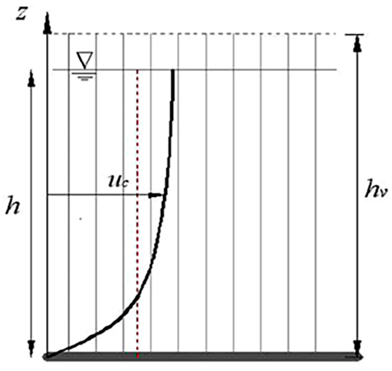
In addition, if there is aquatic vegetation in lakes, the drag effect of vegetation on the water body should be considered as an external force [8,28]. A large amount of vegetation is distributed in Baihe Lake, where reeds and bulrush are dominant [29]. This type of aquatic vegetation shown in Figure 2 with high toughness is generally higher than the water free surface and can be simplified as unsubmerged rigid vegetation [29,30]. A rigid vegetation model based on two-dimensional shallow water equations is presented in Reference [8]. The model treated the unsubmerged rigid vegetation as vertical cylinders and the drag force can be expressed as:

$$S_{vi}=-\frac{1}{2}\lambda C_{d}h{u}_{vi}\sqrt{u_{vj}{u}_{vj}}$$

(6)

where u_vi is the average velocity on the vegetation elements in the i direction; C_d is the drag force coefficient and is usually in the range of 1 and 1.5 [31]; and λ is the projected area (normal to the flow) of vegetation per unit volume of water and is calculated by:

$$\lambda =\frac{4{\alpha }_{v}c}{\pi D_v}$$

(7)

where α_v represents the shape factor; c is the density of the vegetation zones and represents the projected area of vegetation per unit bed area; D_v is the vegetation stems diameter; and u_vi is equal to the average velocity u_i.

2.4. Lattice Boltzmann Method (LBM)

The LBM is a modern numerical technique for computational fluid dynamics. The LBM for non-linear two-dimensional shallow water equations has been widely used [10]. It is a discrete computational method based on the lattice gas automata—a simplified, fictitious molecular model. The three main components in the LBM are lattice pattern, kinetic equation, and equilibrium distribution. The lattice Boltzmann equation can be expressed as:

$$f(x+e_{\alpha }\Delta t,t+\Delta t)=f_{\alpha }(x,t)-\frac{1}{{\tau }_t}[f_{\alpha }(x,t)-f_{\alpha }^{eq}(x,t)]+\Delta t{F}_{\alpha }$$

(8)

where f_α is the particle distribution function; ∆x is the lattice size; ∆t is time step; the external force F_α is calculated by:

$$F_{\alpha }=3{\omega }_{\alpha }\frac{1}{e^2}{e}_{\alpha i}{F}_i$$

(9)

where F_i is force term computed by Equation (3); e = Δx/Δt; ω_α is the weight factor: ω_α = 4/9 for α = 0; ω_α = 1/9 for α = 1, 3, 5, 7; and ω_α = 1/36 for α = 2, 4, 6, 8.

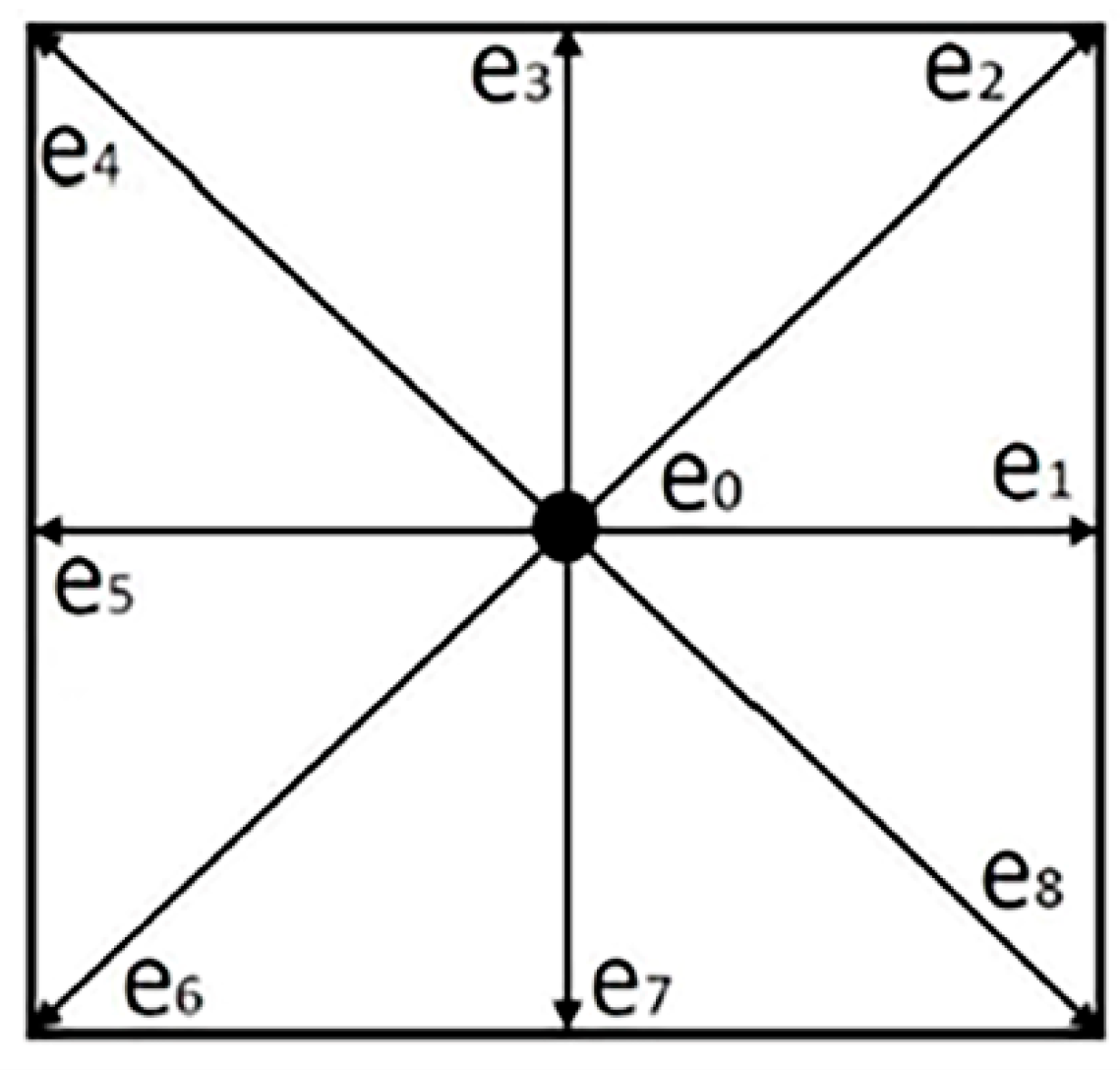
Lattice pattern in the LBM has two functions: indicating grid points and resolving particle motions. The former represents a similar role in the traditional numerical simulation methods. The latter shows a microscopic model for molecular dynamics. e_αi is the particle velocity in the i direction. The nine-velocity square lattice is shown in Figure 3. Each particle moves one lattice unit at its velocity along the eight links represented by numbers 1–8, while 0 represents a particle at rest with zero speed. The velocity vector of the particles is defined by:

$$e_{\alpha }=\{\begin{array}{ll}(0,0)& \alpha =0\\ e\left[\cos \frac{(\alpha -1)\pi }{4},\sin \frac{(\alpha -1)\pi }{4}\right]& \alpha =1,3,5,7\\ \sqrt{2}e\left[\cos \frac{(\alpha -1)\pi }{4}, \sin \frac{(\alpha -1)\pi }{4}\right]& \alpha =2,4,6,8\end{array}$$

(10)

A local equilibrium distribution function decides what flow equations are solved by means of the lattice Boltzmann equation. For 2D shallow water Equations (1) and (2), the local equilibrium distribution function $f_{\alpha }^{eq}$ is defined as:

$$f_{\alpha }^{eq}=\{\begin{array}{ll}h-\frac{5g{h}^2}{6e^2}-\frac{2h}{3e^2}{u}_i{u}_i,& \alpha =0\\ \frac{g{h}^2}{6e^2}+\frac{h}{3e^2}{e}_{\alpha i}{u}_i+\frac{h}{2e^4}{e}_{\alpha i}{e}_{\alpha j}{u}_i{u}_j-\frac{h}{6e^2}{u}_i{u}_i,& \alpha =1,3,5,7\\ \frac{g{h}^2}{24e^2}+\frac{h}{12e^2}{e}_{\alpha i}{u}_i+\frac{h}{8e^4}{e}_{\alpha i}{e}_{\alpha j}{u}_i{u}_j-\frac{h}{24e^2}{u}_i{u}_i,& \alpha =2,4,6,8\end{array}$$

(11)

Then the remaining task is to determine the physical quantities. The macroscopic variables, water depth h and flow velocity u_i can be expressed as:

$$h={\displaystyle \sum _{\alpha }{f}_{\alpha }},u_i=\frac{1}{h}{\displaystyle \sum _{\alpha }{e}_{\alpha i}{f}_{\alpha }}$$

(12)

2.5. Rainfall

Rainfall has an effect on the surface water and runoff, causes soil erosion and floods, and contaminants transport. A numerical model should be applied to investigate how rainfall influences water flow [32]. In the LBM, the local equilibrium distribution function $g_{\alpha }^{eq}$ for shallow water equations with source term was developed. It can be expressed as follows:

$$g_{\alpha }^{eq}=\{\begin{array}{ll}h-R\Delta t-\frac{5g{h}^2}{6e^2}-\frac{2h}{3e^2{u}_i{u}_i}& \alpha =0\\ \frac{g{h}^2}{6e^2}+\frac{h}{3e^2}{e}_{\alpha i}{u}_i+\frac{h}{2e^2}{e}_{\alpha i}{e}_{\alpha j}{u}_i{u}_j-\frac{h}{6e^2}{u}_i{u}_j& \alpha =1,3,5,7\\ \frac{g{h}^2}{24e^2}+\frac{h}{12e^2}{e}_{\alpha i}{u}_i+\frac{h}{8e^2}{e}_{\alpha i}{e}_{\alpha j}{u}_i{u}_j-\frac{h}{24e^2}{u}_i{u}_j& \alpha =2,4,6,8\end{array}$$

(13)

where R is the rainfall intensity and the influence of dynamic pressure caused by precipitation is neglected.

2.6. Boundary Conditions

A general treatment at the inlet is to set a constant velocity and a water depth, whereas a specific water depth is imposed at the outlet. In addition, a zero-gradient condition is used to obtain the velocity components u and v at the outlet. The standard bounce-back scheme, in which an incoming particle towards the boundary is bounced back into the fluid, is widely used. At the upper boundary:

$$f_6=f_2,f_7=f_3,f_8=f_4$$

(14)

and at the lower boundary:

$$f_2=f_6,f_3=f_7,f_4=f_8$$

(15)

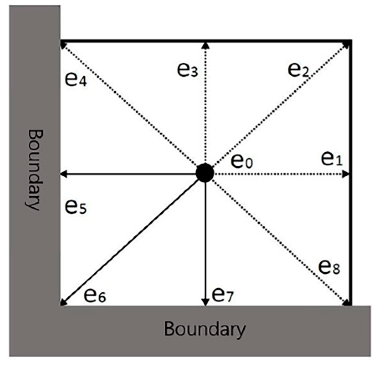
The grids in the corner are involved with changes in boundary conditions, as shown in Figure 4. At the boundary corner point, there will be multiple directions without particle input due to the proximity of the model boundary. It cannot be calculated using the bounce-back scheme or macro variable boundary conditions. It is necessary to calculate the missing particle distribution according to the depth and velocity of the adjacent grids. The computational formula can be expressed as:

$$\{\begin{array}{l}{f}_1=\frac{2h_{x+1,y+1}{u}_{x,y}}{3e}+f_5,\\ f_2=f_6+\frac{h_{x+1,y+1}{u}_{x,y}}{6e}+\frac{h_{x+1,y+1}{v}_{x,y}}{2e},\\ f_3=f_7,\\ f_4=\frac{1}{2}(h_{x+1,y+1}-f_1-f_2-f_3-f_5-f_6-f_7-f_9),\\ f_8=f_4.\end{array}$$

(16)

3. Results

3.1. Initial Conditions

Based on data from 2017, the drainage of farmland converged towards the lake inlet and discharged into Baihe Lake at an average rate of 26.5 m³/s from 11 May to 25 June, and at an average rate of 14.4 m³/s from 10 October to 21 November. The average wind speed was equal to 1.78 m/s in the northeast (132°) from 11 May to 25 June, and average wind speed was equal to 2.36 m/s in the northeast (110°) from 10 October to 21 November.

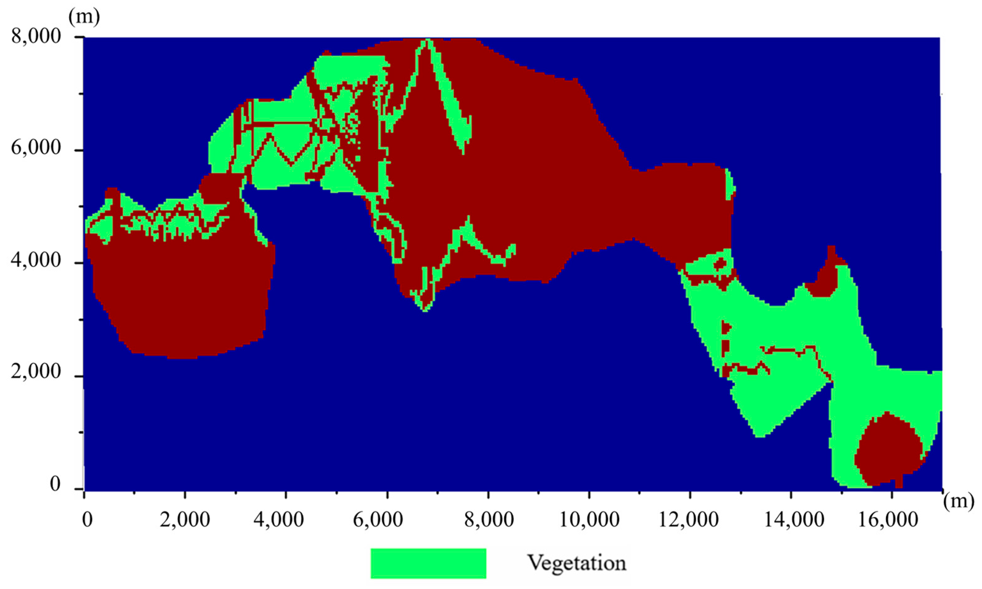
Figure 5 shows the vegetation distribution obtained by a geographic information system and a field investigation. There are a large number of reeds in Baihe Lake that are higher than the water surface and have high rigidity. From inspection of Figure 5, it can be seen that the vegetation is mainly distributed in the northwest and southeast regions of the lake. Based on a field survey, it was found that the vegetation density varies significantly throughout the year. The density is highest from July to August and lowest from January to March. In order to confirm the effect of drag force caused by the vegetation, two situations involving high- and low-vegetation density were tested in the present model. In the computation, the vegetation element shape factor and drag coefficient C_d are equal to 1.0 [28].

3.2. Numerical Tests

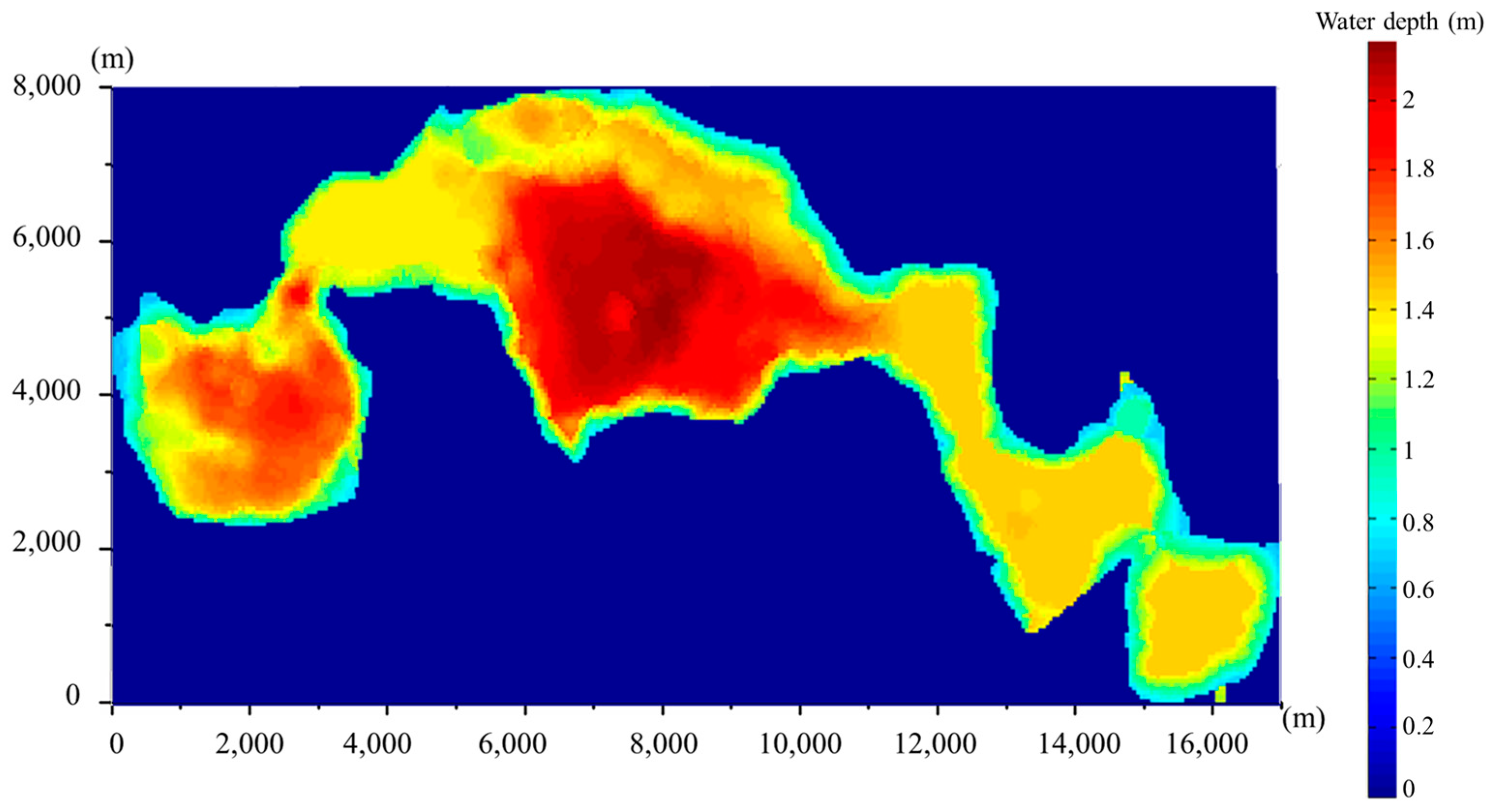
A 2D hydrodynamic model was established using the LBM. Baihe Lake is covered by 340 × 161 grids with each lattice being 50 m × 50 m. The inflow velocity from the northeast inlet is given by 0.5 m/s, which is controlled by sluice gate. The initial water depth in June is shown in Figure 6. Overall, the water depth in the western and eastern regions was relatively shallow compared to the middle region. The average water depth was 1.4 m, and the deepest area was 2.14 m.

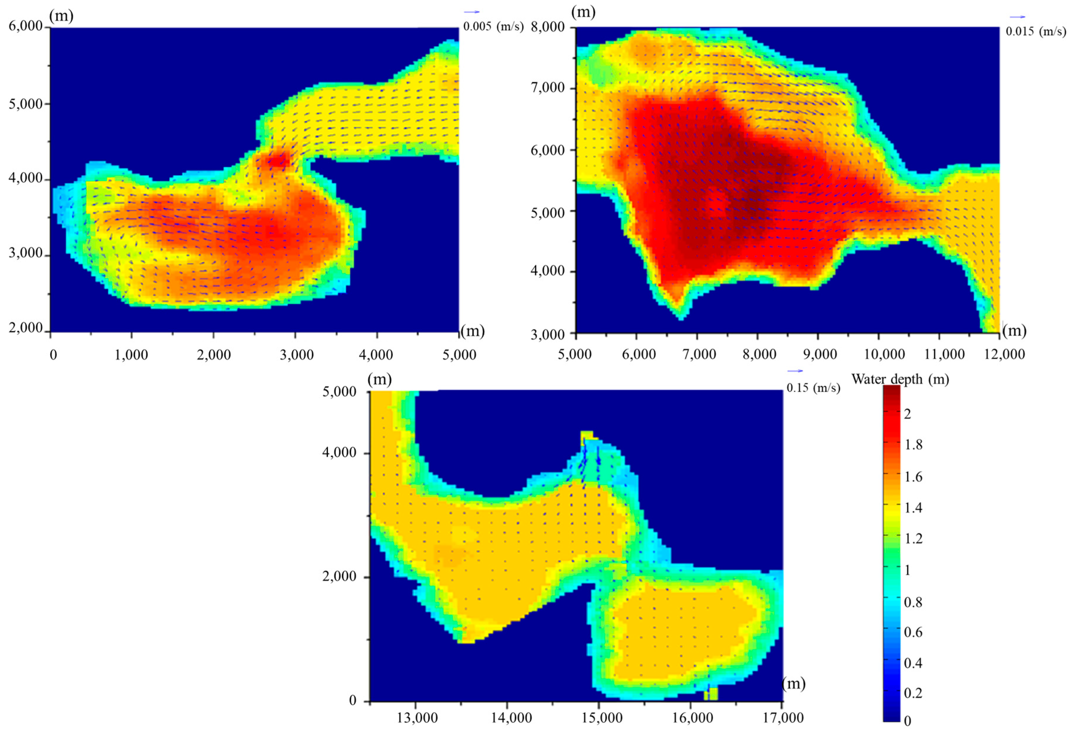
In order to discuss the hydrodynamic characteristics of the lake, the present study simulated the flow field with time from one day to five days. Figure 7 presents the flow field in Baihe Lake after five days for vegetation density c = 0.2. The western region of the lake is far away from the inlet, resulting in a very small flow velocity. The average velocity is about 0.0016 m/s, with an average water depth of 1.32 m. The middle region of the lake is the main area for local fishery. It has sparse vegetation and a larger water depth. The average velocity is about 0.36 cm/s, with an average water depth of 1.89 m. A large amount of vegetation is distributed in the southeast region of the lake. The velocity of the flow is small except for the areas near the outlet or the inlet where the velocities are about 26 cm/s and 0.063 m/s, respectively. The average velocity in the east area is about 0.32 cm/s.

3.3. Sensitivity Analysis

3.3.1. Wind Speed

The wind speed in the Momoge Wetland varies all year round. As a result, it is necessary to investigate the flow field under different wind conditions. The wind speed in the northeast direction was varied by 10%, 20%, 30%, −10%, −20%, and −30%. The flow field became steady after the running time reached five days. The simulation results revealed that the greater the wind speed, the greater the velocity. Wind speed fluctuated by 30%, the outflow velocity varied by 18.77%, and the average velocity of the whole lake varied by 22.16% (see

Table 1. Effect of wind speed on flow velocity.

Variation Range	Wind Speed (m/s)	Outflow Velocity (m/s)	Outflow Velocity Variation	Average Velocity (m/s)	Average Velocity Variation
−30%	1.25	0.0381	−5.93%	0.00149	−7.18%
−20%	1.42	0.0386	−4.69%	0.00152	−5.01%
−10%	1.60	0.0395	−2.47%	0.00155	−2.98%
0%	1.78	0.0405	0.00%	0.00160	0.00%
10%	1.96	0.0411	1.48%	0.00164	2.55%
20%	2.14	0.0433	6.91%	0.00172	7.81%
30%	2.31	0.0457	12.84%	0.00184	14.98%

).

3.3.2. Inflow Discharge

The inflow discharge is significantly affected by drainage from farmlands around the Momoge Wetland and varies across the seasons. The variation percentage of the inflow discharge was varied by 10%, 20%, 30%, −10%, −20%, and −30%. The velocity at the outlet and the flow field in Baihe Lake were the focus. The simulation results revealed a significant positive correlation between inflow and outflow velocity. Due to the strong drag effect of the reeds, a 30% fluctuation in inflow velocity could give rise to only up to 24.11% variation in outflow velocity. Average velocity in the whole lake varied from −21.99% to 27.65% (see

Table 2. Effect of inflow velocity on flow velocity.

Variation Range	Inflow Discharge (m3/s)	Outflow Velocity (m/s)	Outflow Velocity Variation	Average Velocity (m/s)	Average Velocity Variation
−30%	18.55	0.0338	−16.56%	0.00125	−21.99%
−20%	21.20	0.0358	−11.53%	0.00137	−14.58%
−10%	23.85	0.0370	−8.71%	0.00144	−10.24%
0%	26.50	0.0405	0.00%	0.00160	0.00%
10%	29.15	0.0436	7.66%	0.00178	11.42%
20%	31.80	0.0467	15.23%	0.00188	17.63%
30%	34.45	0.0503	24.11%	0.00204	27.65%

).

3.3.3. Vegetation Density

There is a large amount of aquatic vegetation distributed in Baihe Lake. Aquatic vegetation density becomes higher in summer but lower in autumn and winter. The simulation results revealed that there was a negative correlation between vegetation density and outflow velocity. The velocity with higher vegetation density was slower than that with lower density. In addition, a 30% density fluctuation would result in around −5% variation in outflow velocity, which indicates that the vegetation drag force can affect the water flow. Meanwhile, because of the uneven distribution of vegetation, more vegetation is distributed at the inlet and outlet. The average velocity in the whole lake varied from −3.72% to 2.97%, and was less than the variation at the outlet (see

Table 3. Effect of vegetation density on flow velocity.

Variation Range	Vegetation Density	Outflow Velocity (m/s)	Outflow Velocity Variation	Average Velocity (m/s)	Average Velocity Variation
−30%	0.14	0.0424	4.71%	0.00165	2.97%
−20%	0.16	0.0417	3.03%	0.00164	2.57%
−10%	0.18	0.0411	1.49%	0.00162	1.09%
0%	0.20	0.0405	0.00%	0.00160	0.00%
10%	0.22	0.0399	−1.57%	0.00158	−1.23%
20%	0.24	0.0392	−3.11%	0.00155	−2.98%
30%	0.26	0.0385	−4.88%	0.00154	−3.72%

).

3.3.4. Rain Density

Due to the temperate continental climate, rainfall is less in autumn compared to summer. Therefore, the effect of rainfall on the flow field should be considered. The changes in rain density were 10%, 20%, 30%, −10%, −20%, and −30%. The flow field became steady when the simulation time reached five days. The simulation results revealed a positive correlation between rainfall density and outflow velocity. The outflow velocity varied from −14.23% to 21.11%, and the average velocity in the flow field varied from −14.17% to 20.44% (see

Table 4. Effect of rainfall on flow velocity.

Variation Range	Rainfall (mm)	Outflow Velocity (m/s)	Outflow Velocity Variation	Average Velocity (m/s)	Average Velocity Variation
−30%	50.82	0.0347	−14.23%	0.00137	−14.17%
−20%	58.08	0.0370	−8.56%	0.00147	−8.34%
−10%	65.34	0.0385	−4.78%	0.00153	−4.66%
0%	72.60	0.0405	0.00%	0.00160	0.00%
10%	79.86	0.0433	6.97%	0.00171	6.85%
20%	87.12	0.0446	10.23%	0.00176	9.98%
30%	94.38	0.0490	21.11%	0.00193	20.44%

).

3.4. Scenario Simulation

Scenario simulations of different seasons were also run using data from July 2017 and September 2017.

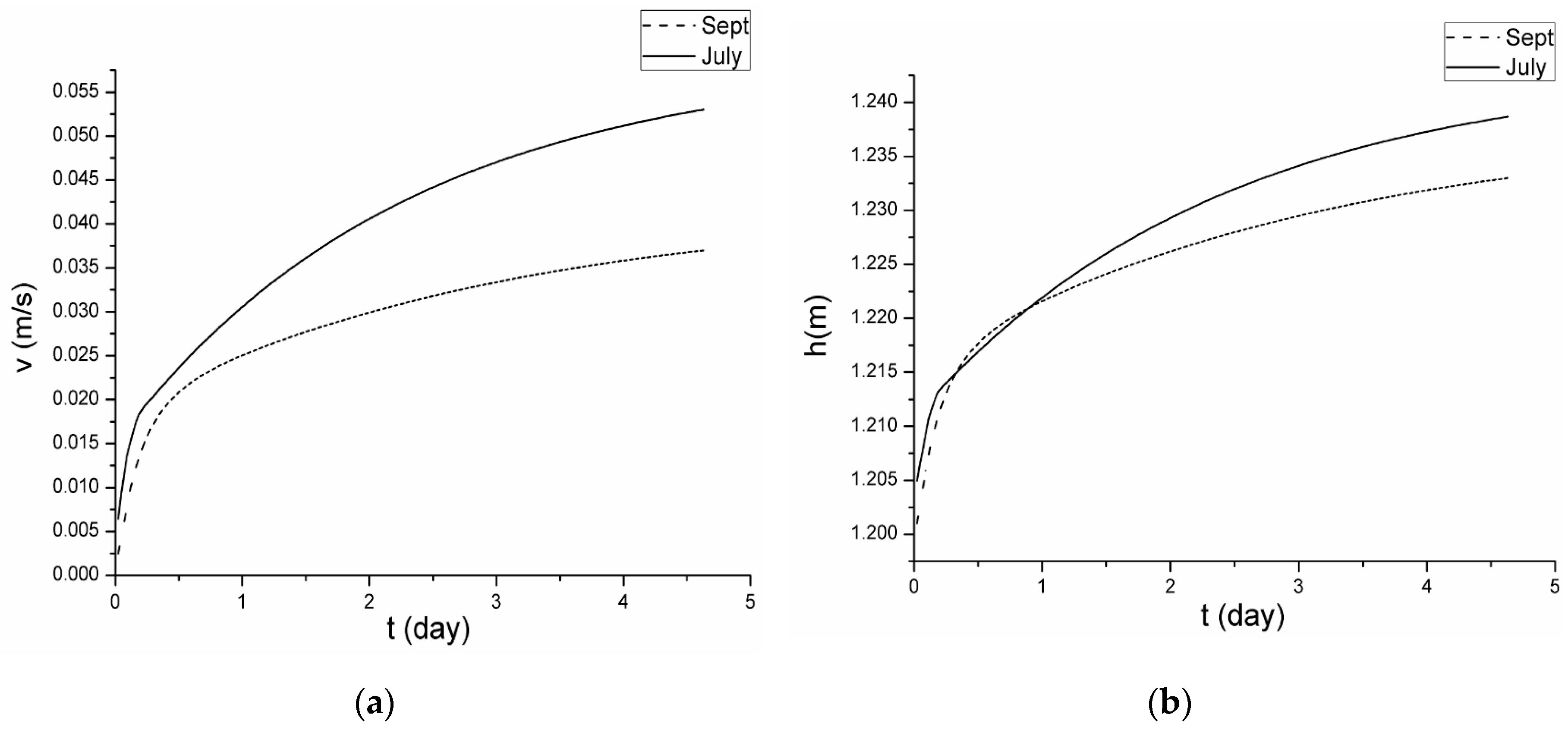
In July 2017, the peak inflow discharge of the drainage from the surrounding farmland was 32 m³/s. The monthly rainfall was 184 mm; the average wind speed was 2.13 m/s in the northeast direction (132°); and the vegetation density was 0.26. When the simulation was stable and the result was steady, the outflow rate was 0.54 m/s. The change in velocity and depth is shown in Figure 8a.

In September 2017, the inflow discharge was 12.6 m³/s in the receding trough of the farmland drainage. The monthly rainfall was 38 mm; the average wind speed was 2.85 m/s in the northeast direction (110°); and the vegetation density was 0.12. The change in velocity and depth is shown in Figure 8b.

4. Discussion

In this paper, the LBM method is applied to Baihe Lake to reveal the temporal and spatial characteristics of water body. Overall, the water body of Baihe Lake suffered poor exchange, where the lowest flow rate based on simulation reached just 0.016 m/s. Simulations of different impact factors (e.g., wind speed, rainfall, vegetation density) were conducted here. The simulation results revealed that changes in inflow velocity, primarily as the result of water drainage from surrounding farmland, have the strongest effect. A 30% variation in the impact factors resulted in a 24.11% variation in the outflow rate at most. In addition, when the impact of wind speed was relatively small, the variation of the outflow rate reached just 18.87%. Relatedly, given the high distribution of aquatic vegetation in some areas of Baihe Lake, and that vegetation density varies with the season, the impact of vegetation on the flow field should be considered separately. The present model includes the change in vegetation density and investigates its effect on the flow fields. The simulation result revealed that vegetation density was negatively correlated with outflow rate. However, the influence of aquatic vegetation on flow distribution was relatively small, being only 9.59% when the vegetation density fluctuated 30%. On the whole, the outflow of Baihe Lake strongly depends on the drainage from upstream farmland, followed by the rainfall, and then by local wind speed. Aquatic vegetation can also have an impact. The inflow rate is the only factor that is easy to control. As a result, ecological protection and hydraulic engineering construction can be established upstream to control the water level and flow rate.

The monitored rainfall, wind speed, flowrate, and vegetation density data in different months was input into the present model in order to simulate and obtain the flow characteristics of Baihe Lake in July and September. Although the influence of wind speed and vegetation was relatively small in the single factor analysis, they can still have an impact on the flow as these two factors have potential uncertainty due to the change in climate. The monitored data revealed large drainage from the surrounding farmland in July, together with high rainfall. Consequently, based on the simulation results, the impact of wind speed and vegetation density was relatively small. In contrast, a reduction in rainfall with a similar farmland drainage happens in September. Importantly, this increases the influence of wind speed and vegetation density. The results indicated that the mean flow rate is much bigger in July than September, which also verifies the significance of different impact factors. Relatedly, the simulation results also demonstrate that the water exchange of Baihe Lake during the flood season from June to August is much better than it is in the dry season from September to November. Therefore, when developing an ecological restoration program, both the farmland drainage and the season should be emphasized.

5. Conclusions

Based on the lattice Boltzmann method (LBM), the present study has established a two-dimensional shallow water model that includes vegetation drag force. This paper for the first time puts forward a method to study the variation of flow field by establishing a numerical model of the Baihe Lake, which plays a guiding role in the construction of the ecological engineering of the Baihe Lake. The hydrodynamic model in this paper can be widely used in shallow lakes. Meanwhile, the drag force of aquatic vegetation to Baihe Lake is specially considered in the model, leading to that the model is most suitable for lakes with aquatic vegetation.

The model was used to explore the hydrodynamic impact of different influencing factors in Baihe Lake. Through a sensitivity test, drainage from surrounding farmland showed a dominant influence on the flow field, followed by rainfall, wind speed, and vegetation density. Furthermore, these factors may produce a noticeable variation in local flow characteristics in different seasons. As a result, the impact of these factors should be considered when developing an ecological restoration program. We should pay attention to different schemes corresponding to different seasons and control hydraulic construction to influence farmland receding water and improve lake fluidity.

References

- Zeng, L.; Chen, G.Q. Flow distribution and environmental dispersivity in a tidal wetland channel of rectangular cross-section. Commun. Nonlinear Sci. 2009, 17, 4192–4209. [Google Scholar] [CrossRef]
- Calhoun, A.J.; Mushet, D.M.; Bell, K.P.; Boix, D.; Fitzsimons, J.A.; Isselin-Nondedeu, F. Temporary wetlands: Challenges and solutions to conserving a ‘disappearing’ ecosystem. Biol. Conserv. 2017, 211, 3–11. [Google Scholar] [CrossRef]
- Hui, F.; Xu, B.; Huang, H.; Yu, Q.; Gong, P. Modelling spatial-temporal change of Poyang Lake using multitemporal Landsat imagery. Int. J. Remote. Sens. 2008, 29, 5767–5784. [Google Scholar] [CrossRef]
- Yang, R.; Cui, B. A wetland network design for water allocation based on environmental flow requirements. Clean Soil Air Water 2012, 40, 1047–1056. [Google Scholar] [CrossRef]
- Stephan, U.; Gutknecht, D. Hydraulic resistance of submerged flexible vegetation. J. Hydrol. 2002, 269, 27–43. [Google Scholar] [CrossRef]
- Kouwen, N. Friction factors for coniferous tress along rivers. J. Hydraul. Eng. 2000, 126, 732–740. [Google Scholar] [CrossRef]
- Huai, W.X.; Zeng, Y.H.; Xu, Z.G. Three-layer model for vertical velocity distribution in open channel flow with submerged rigid vegetation. Adv. Water. Resour. 2009, 32, 487–492. [Google Scholar] [CrossRef]
- Yang, Z.; Bai, F.; Huai, W.; An, R.; Wang, H. Modelling open-channel flow with rigid vegetation based on two-dimensional shallow water equations using the lattice Boltzmann method. Ecol. Eng. 2017, 106, 75–81. [Google Scholar] [CrossRef]
- Yang, S.; Bai, Y.; Xu, H. Experimental analysis of river evolution with riparian vegetation. Water 2018, 10, 1500. [Google Scholar] [CrossRef]
- Zhou, J.G. A lattice Boltzmann model for the shallow water equations. Int. J. Mod. Phys. C 2002, 13, 1135–1150. [Google Scholar] [CrossRef]
- Liu, Q.; Qin, Y.; Zhang, Y.; Li, Z. A coupled 1D–2D hydrodynamic model for flood simulation in flood detention basin. Nat. Hazards 2015, 75, 1303–1325. [Google Scholar] [CrossRef]
- Patro, S.; Chatterjee, C.; Mohanty, S.; Singh, R.; Raghuwanshi, N.S. Flood inundation modeling using MIKE FLOOD and remote sensing data. J. Indian Soc. Remote Sens. 2009, 37, 107–118. [Google Scholar] [CrossRef]
- Arifin, R.R.; James, S.C.; de Alwis Pitts, D.A.; Hamlet, A.F.; Sharma, A.; Fernando, H.J. Simulating the thermal behavior in Lake Ontario using EFDC. J. Great Lakes Res. 2016, 42, 511–523. [Google Scholar] [CrossRef]
- Bai, H.; Chen, Y.; Wang, D.; Zou, R.; Zhang, H.; Ye, R.; Ma, W.; Sun, Y. Developing an EFDC and numerical source-apportionment model for nitrogen and phosphorus contribution analysis in a Lake Basin. Water 2018, 10, 1315. [Google Scholar] [CrossRef]
- Chen, S.; Doolen, G.D. Lattice Boltzmann method for fluid flows. Ann. Rev. Fluid Mech. 1998, 30, 329–364. [Google Scholar] [CrossRef]
- Succi, S.; Santangelo, P.; Benzi, R. High-resolution lattice-gas simulation of two-dimensional turbulence. Phys. Rev. Lett. 1988, 60, 2738–2740. [Google Scholar] [CrossRef] [PubMed]
- Salmon, R. The lattice Boltzmann method as a basis for ocean circulation modeling. J. Mar. Res. 1999, 57, 503–535. [Google Scholar] [CrossRef]
- Dellar, P.J. Non-hydrodynamic modes and a priori construction of shallow water lattice Boltzmann equations. Phys. Rev. E 2002, 65, 036309. [Google Scholar] [CrossRef]
- Liu, H.; Ding, Y.; Wang, H.; Zhang, J. Lattice Boltzmann method for the age concentration equation in shallow water. J. Comput. Phys. 2015, 299, 613–629. [Google Scholar] [CrossRef]
- Liu, H.; Zhou, J.G. Inlet and outlet boundary conditions for the Lattice-Boltzmann modelling of shallow water flows. Prog. Comput. Fluid. Dyn. 2012, 12, 11–18. [Google Scholar] [CrossRef]
- Ottolenghi, L.; Prestininzi, P.; Montessori, A.; Adduce, C.; La Rocca, M. Lattice Boltzmann simulations of gravity currents. Eur. J. Mech. B-Fluid 2018, 67, 125–136. [Google Scholar] [CrossRef]
- O’Brien, G.S.; Bean, C.J.; Mcdermott, F. A comparison of published experimental data with a coupled lattice Boltzmann-analytic advection–diffusion method for reactive transport in porous media. J. Hydrol. 2002, 268, 143–157. [Google Scholar] [CrossRef]
- Zhou, J.G. A rectangular lattice Boltzmann method for groundwater flows. Mod. Phys. Lett. B 2007, 21, 531–542. [Google Scholar] [CrossRef]
- Tubbs, K.R.; Tsai, T.C. Multilayer shallow water flow using lattice Boltzmann method with high performance computing. Adv. Water. Resour. 2009, 32, 1767–1776. [Google Scholar] [CrossRef]
- Liu, H.; Li, M.; Shu, A. Large eddy simulation of turbulent shallow water flows using multi-relaxation-time lattice Boltzmann model. Int. J. Numer. Meth. Fluids 2012, 70, 1573–1589. [Google Scholar] [CrossRef]
- Prestininzi, P.; Montessori, A.; Rocca, M.; Sciortino, G. Simulation of arrested salt wedges with a multi-layer Shallow Water Lattice Boltzmann model. Adv. Water Resour. 2016, 96, 282–289. [Google Scholar] [CrossRef]
- Chávarri, E.; Crave, A.; Bonnet, M.P.; Mejía, A.; Da Silva, J.S.; Guyot, J.L. Hydrodynamic modelling of the Amazon River: Factors of uncertainty. J. S. Am. Earth. Sci. 2013, 44, 94–103. [Google Scholar] [CrossRef]
- Stone, B.M.; Shen, H.T. Hydraulic resistance of flow in channels with cylindrical roughness. J. Hydraul. Eng. 2002, 128, 500–506. [Google Scholar] [CrossRef]
- Konings, A.G.; Katul, G.G.; Thompson, S.E. A phenomenological model for the flow resistance over submerged vegetation. Water. Resour. Res. 2012, 48, 2478. [Google Scholar] [CrossRef]
- Poggi, D.; Krug, C.; Katul, G.G. Hydraulic resistance of submerged rigid vegetation derived from first-order closure models. Water. Resour. Res. 2009, 45, 2381–2386. [Google Scholar] [CrossRef]
- Guan, M.; Liang, Q. A two-dimensional hydro-morphological model for river hydraulics and morphology with vegetation. Environ. Modell. Softw. 2017, 88, 10–21. [Google Scholar] [CrossRef] [Green Version]
- Ding, Y.; Liu, H.; Peng, Y.; Xing, L. Lattice Boltzmann method for rain-induced overland flow. J. Hydrol. 2018, 562, 789–795. [Google Scholar] [CrossRef]
Figure 1.
Geographical location and topographic conditions of Baihe Lake (Datum: 45°56’ N, 122°45’ E).
Figure 2.
Flow over unsubmerged rigid vegetation.
Figure 3.
D2Q9 lattice pattern (D2 represent two-dimensional and Q9 represent nine velocity directions in each particle).
Figure 4.
Corner grid.
Figure 5.
Vegetation distribution in Baihe Lake.
Figure 6.
Initial water depth in Baihe Lake.
Figure 7.
Water depth and velocity vectors after 5 days.
Figure 8.
Comparison of the simulated results with different initial conditions: (a) Case 1 (water velocity); (b) Case 2 (water depth).