Improving the Performance of Vegetable Leaf Wetness Duration Models in Greenhouses Using Decision Tree Learning

Abstract

Leaf wetness duration (LWD) is a key driving variable for peat and disease control in greenhouse management, and depends upon irrigation, rainfall, and dewfall. However, LWD measurement is often replaced by its estimation from other meteorological variables, with associated uncertainty due to the modelling approach used and its calibration. This study uses the decision learning tree method (DLT) for calibrating four LWD models—RH threshold model (RHM), the dew parameterization model (DPM), the classification and regression tree model (CART) and the neural network model (NNM)—whose performances in reproducing measured data are assessed using a large dataset. The relative importance of input variables in contributing to LWD estimation is also computed for the models tested. The LWD models were evaluated at two different greenhouse locations: in a Chinese (CN) greenhouse over three planting seasons (April 2014–October 2015) and in a Spanish (ES) greenhouse over four planting seasons (April 2016–February 2018). Based on multi-evaluation indicators, the models were given a ranking for their assessment capabilities during calibration (in the Spanish greenhouse from April 2016 to December 2016 and in the Chinese greenhouse from April 2014 to November 2014). The models were then evaluated on an independent set of data, and the obtained areas under the receiver operating characteristic curve (AUC) of the LWD models were over 0.73. Therein, the best LWD model in this case was the NNM, with positive predict values (PPVs) of 0.82 (SP) and 0.90 (CN), and mean absolute errors (MAEs) of 1.85 h (SP) and 1.30 h (CN). Consequently, the DLT can decrease LWD estimation error by calibrating the model threshold and choosing black box model input variables.

1. Introduction

Leaf wetness duration (LWD) is the time of visible water presence on plant surfaces, i.e., the leaves, stems, flowers and fruits [1]. It is caused by over irrigation, rainfall or condensation, and acts as a catalyst for disease onset as it favors fungal infections, therefore causing a high possibility of heavy yield losses. For example, LWD facilitates gray leaf spot dispersal, which is an important fungal disease in maize and tomato [2,3], as it influences the processes of germination, infection, sporulation and, to a lesser extent, the lag time for symptom development (the latent period) [4]. However, leaf wetness duration is not only a meteorological variable, like temperature or precipitation, and it has not been routinely measured by most national meteorological agencies as part of general observation programs [5]. Therefore, different typology model based-weather station data for LWD simulation were developed, and are routinely used to provide inputs to early disease warning systems of disease outbreaks [6,7]. The LWD models can be divided into two broad categories: empirical and physical models. The latter are data demanding because they require inputs that are not always available, such as cloud cover and net radiation [8,9]. Conversely, estimation of LWD is based on its relationships with meteorological variables available in standard agro-meteorological stations. Some examples of empirical LWD models are the simple relative humidity threshold model (RHM), which simulates the leaf wetness occurrence when humidity is above a threshold [10,11]; the dew point depression method (DPM), based on the principle of dew formation [12,13]; and the classification and regression tree (CART) model, which considers the non-linear relationship between leaf wetness, wind speed, rainfall, dew temperature and relative humidity in decision nodes to determine leaf wetness [14]. Kim et al. demonstrated the spatial portability of the CART model through its application in different environments [15]. Gillespie et al. achieved good results when estimating LWD by a dew point depression model [16]. Further attempts have been made for estimation of LWD using neural network models (NNMs), which can be considered black box models. These are self-adaption models trained with reference data, and are widely used to various prediction problems, including temperature [17], leaf area index [18], gray leaf spot on maize [19] and flooding [20]. Before using leaf wetness models operationally, however, they should be compared to analyze their performance, and therefore to help farms in greenhouse management, e.g., to avoid over irrigation, untimely ventilation and disease infection.

When user-defined thresholds or parameters were applied directly in models without calibrating them using local data, their accuracy is largely uncertain. For example, the relative humidity threshold model was used to estimate LWD by Sentelhas et al. [13] for four locations using the same empirical threshold (RH > 90%) and by Mackenzie and Peres [21] for predicting the proportion of infected strawberry fruit in Florida depending on an empirical threshold (RH > 85%). Although Bregaglio et al. [10] proposed a multi-metric evaluation method for comparing the performance of six LWD models contributing to the large-area application of plant disease models in 12 sites across the USA and Italy, limitation of data availability still remains a barrier. Gil et al. proposed that calibration of the relative humidity threshold model can greatly improve its precision in Colombia (threshold at 94%) [22]. The structure of a neural network-based leaf wetness model includes inputs, outputs and intermediate layers. The number of intermediate layers, the elements contained therein, and the connection between the elements are user-selectable; this gives the network flexibility in pattern recognition during model development but leads to alterable results. Determining the most important variables in a model—which to include (and exclude) in the model, and which of the included variables contribute the most to prediction—is critical from both the practical and theoretical perspectives [23]. Francl and Panigrahi [24] analyzed the sensitivity of artificial neural network models of wetness status at the wheat flag leaf level to individual input variables, and estimated that leaf wetness duration and relative humidity were very important factors, as expected, and temperature, solar radiation, and time of day were also influential. Of lesser importance were wind speed and precipitation, but predictions were always correct when it rained. However, Stella et al. [25] proposed the inputs of an artificial neural network (ANN) for estimation of leaf wetness duration of apple trees were air temperature, relative humidity, rainfall, wind speed, and solar radiation..

Data mining algorithms can be used for this purpose. The top 10 data mining algorithms were identified by the Institute of Electrical and Electronic Engineers (IEEE) International Conference on Data Mining, at which it was shown that decision learning trees (DLTs), support vector machines (SVMs), K-means (K-M) and Naive Bayes (NB) are widely used methods for data classification and statistical learning [26]. Considering that leaf wetness occurrence is a binary classification problem and that a robust calibration requires a large dataset, a suitable method needs to be chosen for optimizing threshold or parameters of the models. The K-M is a clustering algorithm to classify unlabeled data using approximate distances between different points on the input vectors. When the leaf wetness model has multiple categories for identifying whether a leaf is dry or wet, as in the CART model, K-M cannot follow the category order to continuously split all data. The SVM and NB methods are frequently used to solve only small sample classifications because of certain disadvantages, namely, the sensitive kernel function and the conditional independence assumptions. Leaf wetness is a complex process dependent on the climate parameters used (relative humidity, dew temperature, air temperature, wind speed, rainfall, radiation) in the models. Therefore, it is difficult to define the weight coefficients of these parameters, which leads to a sensitive kernel function. Decision tree learning is one of the most successful learning algorithms due to its features of simplicity, comprehensibility, and lack of parameters, as well as being able to handle mixed-type data [27]. A class label and a tuple of attributes are used to train labeled data. Its advantage is its vast research space and its recursive processing until all instances in a subset belong to the same class. The calibrated threshold of a leaf wetness model is obtained from the tree node by classifying the objective variable using a class label (wet or dry) and a tuple of attributes (model parameters). The decision learning tree supplies a function to rank predictor importance by totaling the changes in the mean squared error (MSE) caused by the splits for each predictor, and then dividing the total by the number of branch nodes.

This work aims at testing the performances of four LWD models (RHM, DPM, CART and NNM) in two different greenhouse systems in Spain and China, and to compare their accuracy before and after calibration using reference data obtained in dedicated experimental trials.

2. Materials and Methods

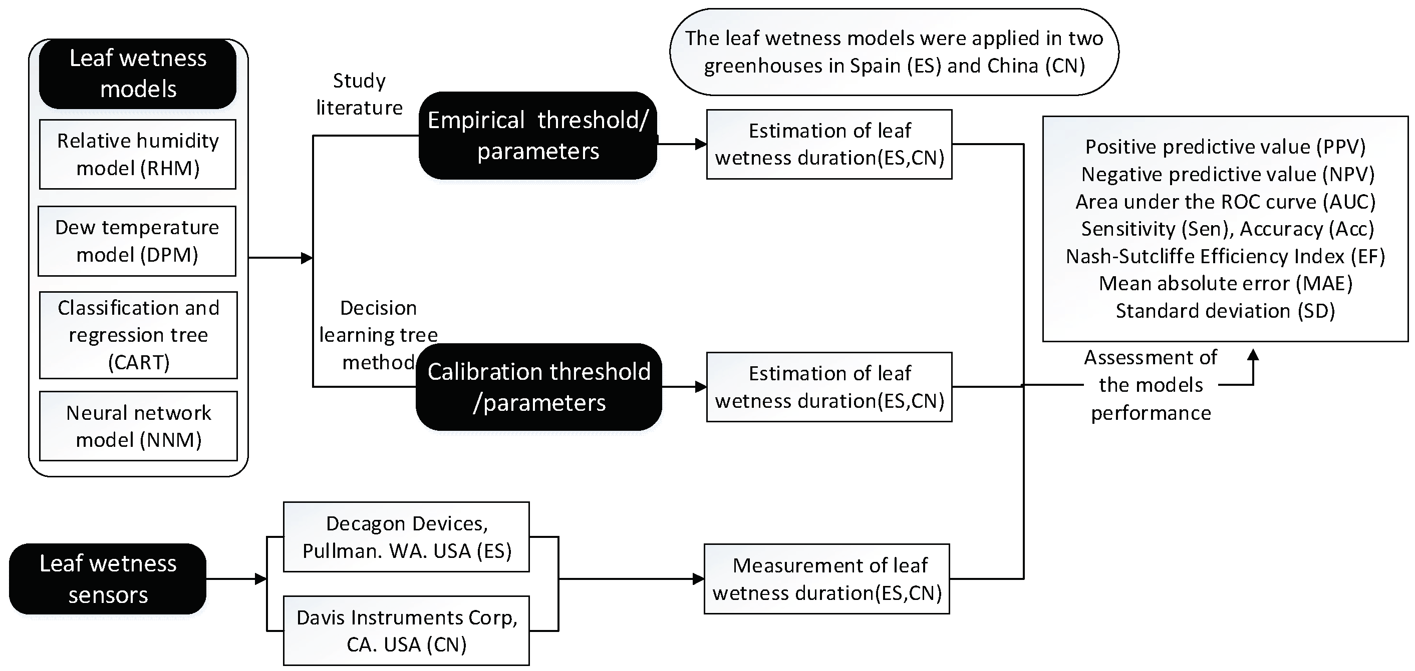
The models tested here were aimed at estimating leaf wetness duration. Four leaf wetness models were applied to data collected in a plastic greenhouse of Almeria, Spain and in a solar greenhouse placed in Beijing, China. The tested models were: a simple relative humidity threshold (RHM), a dew temperature-based model (DPM), a classification and regression tree (CART) and a model based on a neural network (NNM). The choice of using weather and leaf wetness data coming from Spanish and Chinese greenhouses was driven by data availability. The relevance of our procedure is its ease of replicability in different greenhouse conditions, more than in different geographical areas. The classification tree function in MATLAB R2018a was used to calibrate the parameters of the leaf wetness models, and their performances were assessed by the statistical indexes: positive predictive value (PPV), negative predictive value (NPV), area under the receiver operating characteristic curve (AUC) and Nash–Sutcliffe efficiency index (EF), and mean absolute error (MAE) and standard deviation (SD). The workflow is shown in Figure 1.

2.1. Greenhouse Facilities and Leaf Wetness Duration Monitoring

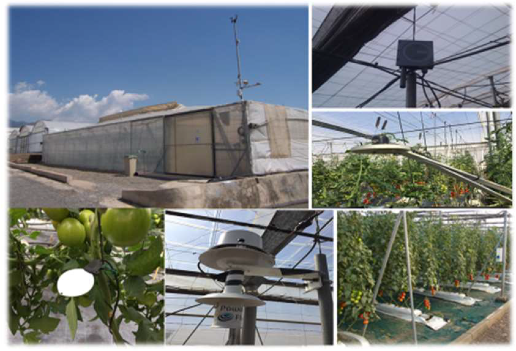
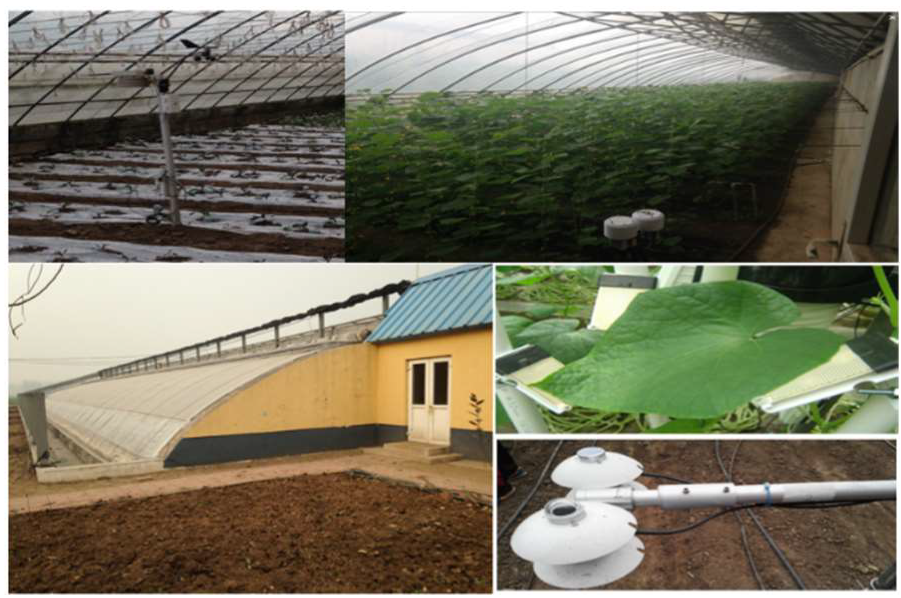
Two greenhouses located in Spain (Figure 2) and China (Figure 3) were used in this study to evaluate the LWD models’ accuracy. In Spain, the greenhouse size was 877 m² (37.8 m × 23.2 m) with a variable height (between 2.8 m and 4.4 m) and a polyethylene cover, whitened to reduce radiation (by the application of a CaCO₃ suspension) based on the external conditions. The tomato crop density was 2.01 plants/m² (6 plants per slab, 1.9 m between slab rows and 0.5 m between slabs in the same row). Two electronic sensors were designed to mimic the size of natural leaves based on obtaining a dielectric constant on the sensor surfaces using a capacitive grid (Decagon Devices, Pullman, WA, USA), and they were installed at the bottom and top of the canopy in the center of the greenhouse at a 30° angle. There was a weather station inside the greenhouse to test the air temperature and air humidity (Vaisala HMP45P, Helsinki, Finland), which was located at the center of the greenhouse at a 2.0 m height. The leaf wetness data were collected from 2016 to 2018. In China, the greenhouse size was 210 m² (30 m × 7 m) and was constructed of metal arches covered with polyethylene film. A total of 504 cucumber plants were arranged in a double-row pattern with small 40 cm spaces and large 1.1 m spaces between rows; there was also a space of 0.4 m between plants in each row. The air temperature and relative humidity in the greenhouse were recorded every 15 min by sensors coupled to a data logger, which was located at the center of the greenhouse at a 1.5 m height. The data were transferred from the data logger (an RS485 connection) to a central computer (an RS232 connection) via a local area network (LAN) and stored in a Microsoft Access 2003 database. Five leaf wetness sensors (#6420, Davis Instruments Corp, Hayward CA, USA) and a data logger (CR1000, Campbell Scientific, Logan, UT, USA) were located at the leaf apex, the left and right side of the leaf, the underside of the leaf and 0.05 m below of the leaf, and were always kept at the middle of the canopy during crop growing [28]. The data were acquired from 2014 to 2015.

The leaf was considered wet when 50% of the sampled data was over the LW sensor threshold for one hour [29]. The differences in the periods of measurements, seasons, measurement intervals and LWD sensors among sites occurred because we used the infrastructure and data available for each place (

Table 1. Greenhouses conditions in Spain and China.

Location and Plant	Greenh-Ouse Type	Area	Plant Density	Leaf Wetness Sensor (Numbers/Series)	Experiment Data	T (°C)	RH (%)	LWD (h)
Tomato, Almeria, Spain	‘Parral’ greenhou-se	37.8 m × 23.2 m	2.01 plants/m2	2/Decagon Devices, Pullman, WA, USA	April 2016–February 2018	22.91	59.86	4.39
Cucumber, Beijing, China	Solar greenhou-se	30 m × 7 m	2.4 plants/m2	5/#6420, Davis Instruments Corp, Hayward CA, USA	April 2014–October 2015	20.35	67.33	6.06

Note: average leaf wetness duration (LWD) was the mean value of leaf wetness durations of leaf wetness occurrence days; T means average of air temperature; RH means average of relative humidity.

).

2.2. Model Description

The four LWD models tested in our study are described below:

1

The RHM assumes the LWD is equal to the number of hours that RH is greater than or equal to a constant threshold. If the RH is below that threshold, the leaves are assumed to be dry; conversely, if the RH is above the threshold, the leaves are assumed to be wet. In this case, we set the empirical threshold to 90% according to the cases of the relative humidity model application in disease warning systems; an optimal RHM threshold (RH ≥ 90%) was used in an existing cucumber downy mildew warning system [11], a strawberry disease-warning systems in four US states [30], and a potato late blight model [31].

2

The DPM is based on the difference value (DPD) between the air temperature (T) and the dew point temperature (dewT) [4]. Dew occurs only when the difference is below a certain threshold (2 °C) [32]. This model was used by Huber and Gillespie [4] and by Gillespie et al. [16]. The same model was also applied in other studies on leaf wetness estimation [13,32]. In this study, we kept the dew point threshold to 2 °C to determine dew presence in the two greenhouse systems.

3

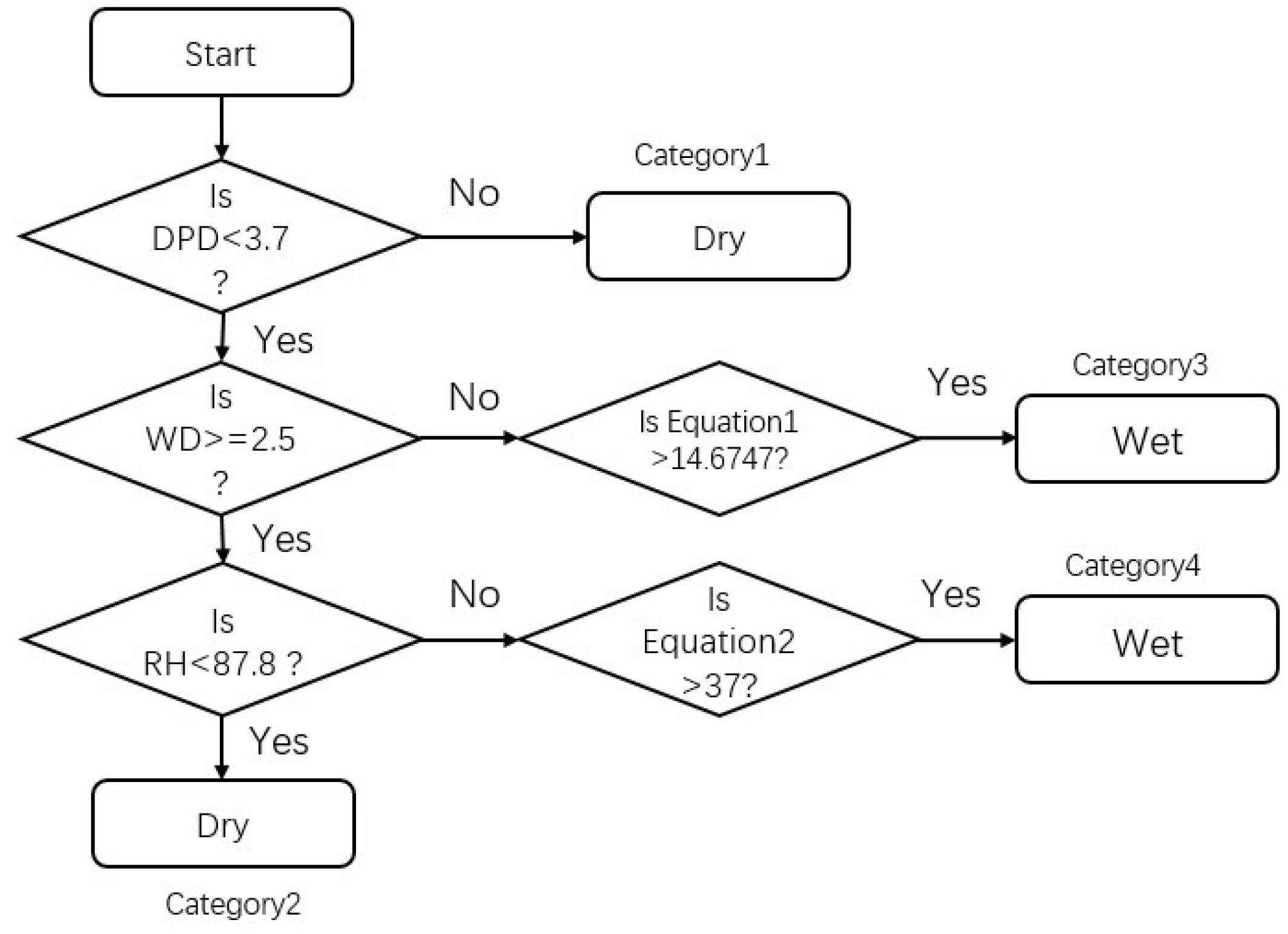
The CART model [33] has four category conditions to identify whether leaves are dry or wet (Figure 4); these are the hours considered dry if either the hourly different value (DPD) is equal or greater than 3.7 °C (category 1) or if the relative humidity (RH) is less than 87.8% and the hourly wind speed (WD) is equal or greater than 2.5 m s⁻¹ (category 2). The hours in category 3 (Equation (1)) and category 4 (Equation (2)) are classified as either dry or wet by a subsequent stepwise linear discriminant analysis.

$$1.6064{\mathrm{T}}^{0.5}+0.0036{\mathrm{T}}^2+0.1531\mathrm{RH}-0.4599\mathrm{WD}\times \mathrm{DPD}-0.0035\mathrm{T}\times \mathrm{RH}>14.4674.$$

(1)

$$0.7921{\mathrm{T}}^{0.5}+0.0046{\mathrm{RH}}^2-2.3889\mathrm{WD}-0.0390\mathrm{T}\times \mathrm{WD}+1.0613\mathrm{WD}\times \mathrm{DPD}>37.0000$$

(2)

4

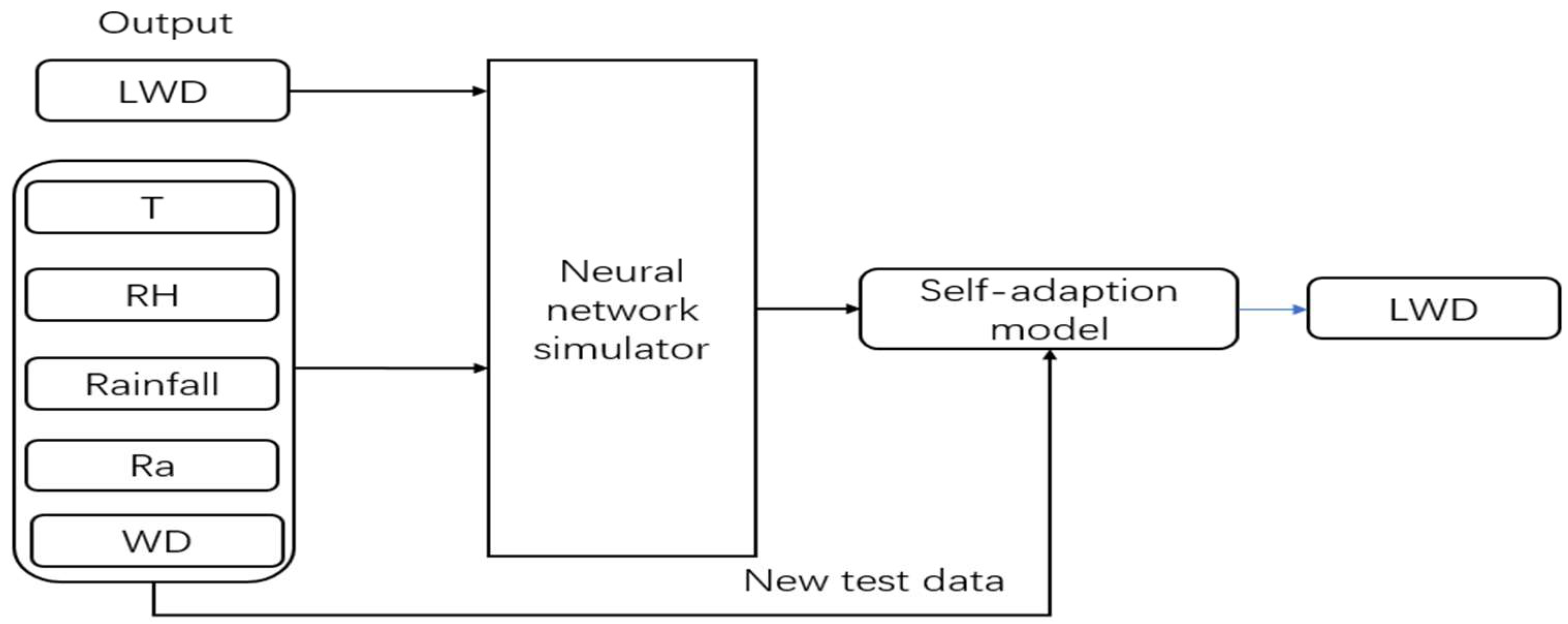
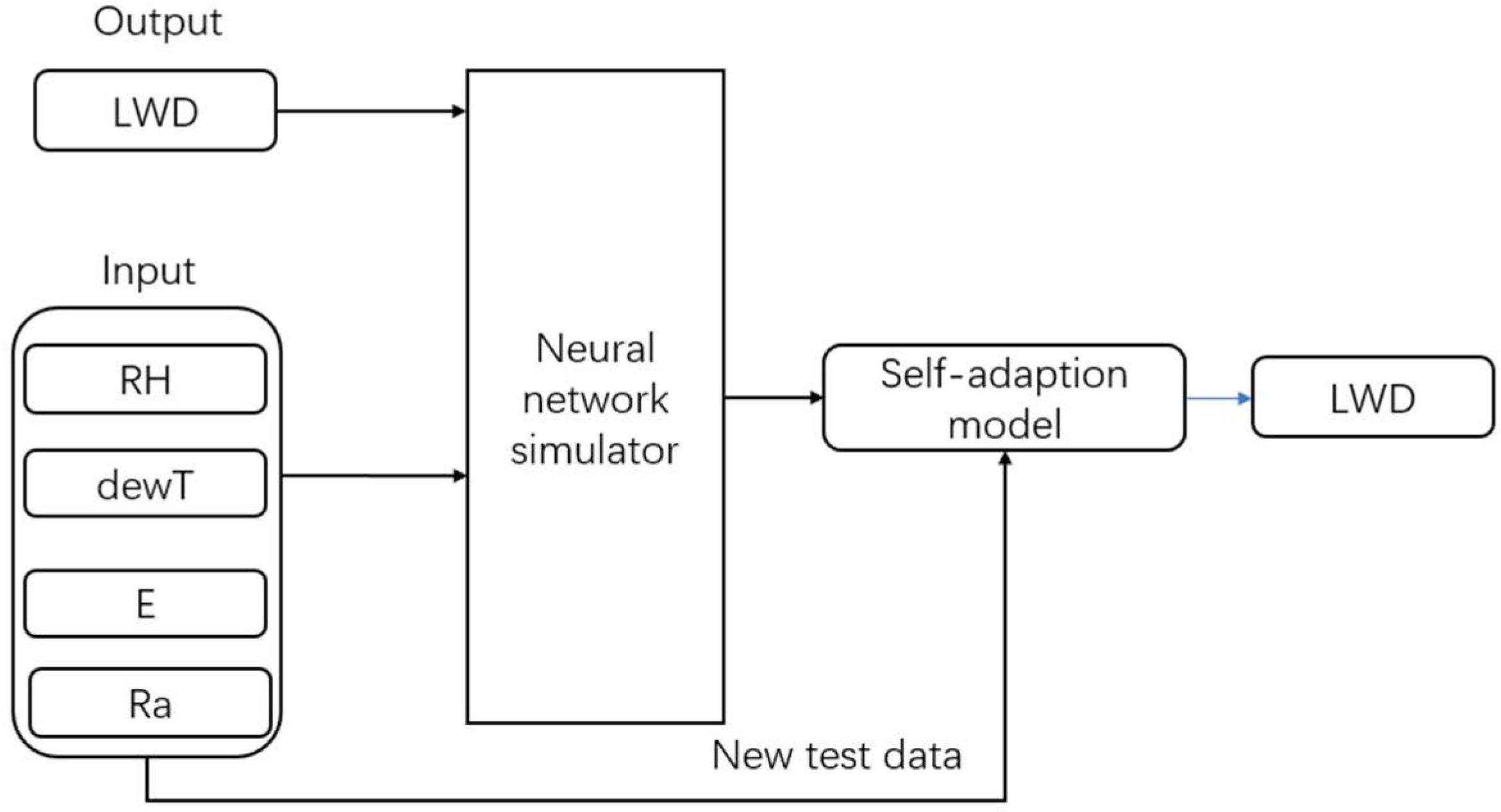
A neural network model (NNM) is a method to predict a set of outputs from a set of input patterns [34]. It is like a central nervous system that can learn tasks by considering examples. Leaf wetness is the output of a neural network-based leaf wetness model [14]. Francl et al. estimated wheat leaf wetness using the inputs of temperature, relative humidity, solar radiation, precipitation, wind direction, and wind speed [24]. Marta et al. carried out the model in 47 weather stations, and its input parameters were rainfall, vapor pressure deficit, wind speed and solar global radiation [29]. Stella et al. [25] used the inputs (temperature, relative humidity, rainfall, wind speed and solar radiation) in a neural network model for estimating apple leaf wetness. We chose the empirical input parameters of NNM that are shown in Figure 5, in which T is temperature (°C); RH is relative humidity (%); DPD is dew point depression (°C); WD is wind speed (m/s) and Ra is global radiation (W²).

The parameters which were calibrated for each leaf wetness models are listed in

Table 2. Calibration parameters in four leaf wetness models.

Models	Relative Humidity Model (RHM)	Dew Temperature Model (DPM)	Classification and Regression Tree (CART)	Neural Network Model (NNM)
Calibration parameters	Relative humidity (RH)	The difference of temperature and dew temperature (DPD)	DPD, Wind speed (WD), RH, the node splitting of Equations (1) and (2)	Input parameters

. The calibration of the four leaf wetness models was performed using the decision learning tree method (DLT), by splitting the available data into two independent sets for calibration and evaluation. For the CART model, we decided to keep the original coefficients of Equations (1) and (2), and to limit its calibration to the thresholds leading to the node splitting (14.4674 in Equation (1), 37 in Equation (2)). Since these equations were derived by data fitting during model development, the values of the empirical coefficients have limited meaning and no portability.

2.3. Decision Learning Tree (DLT) Method

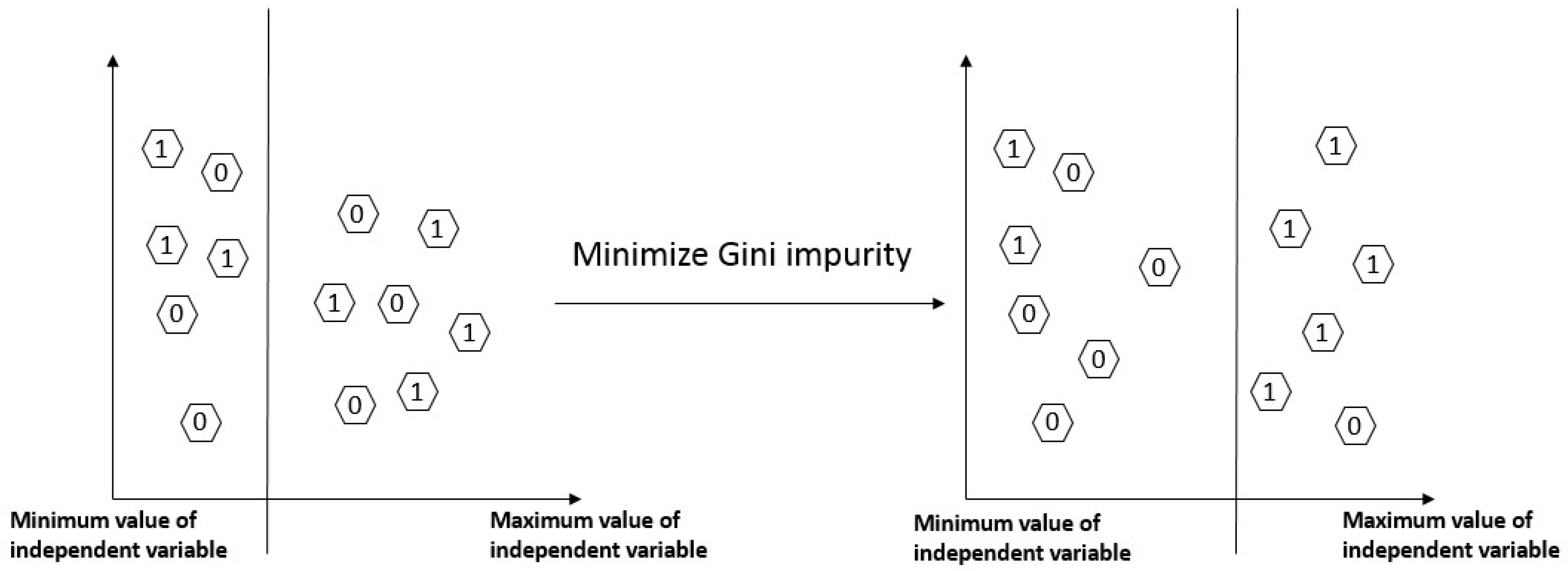
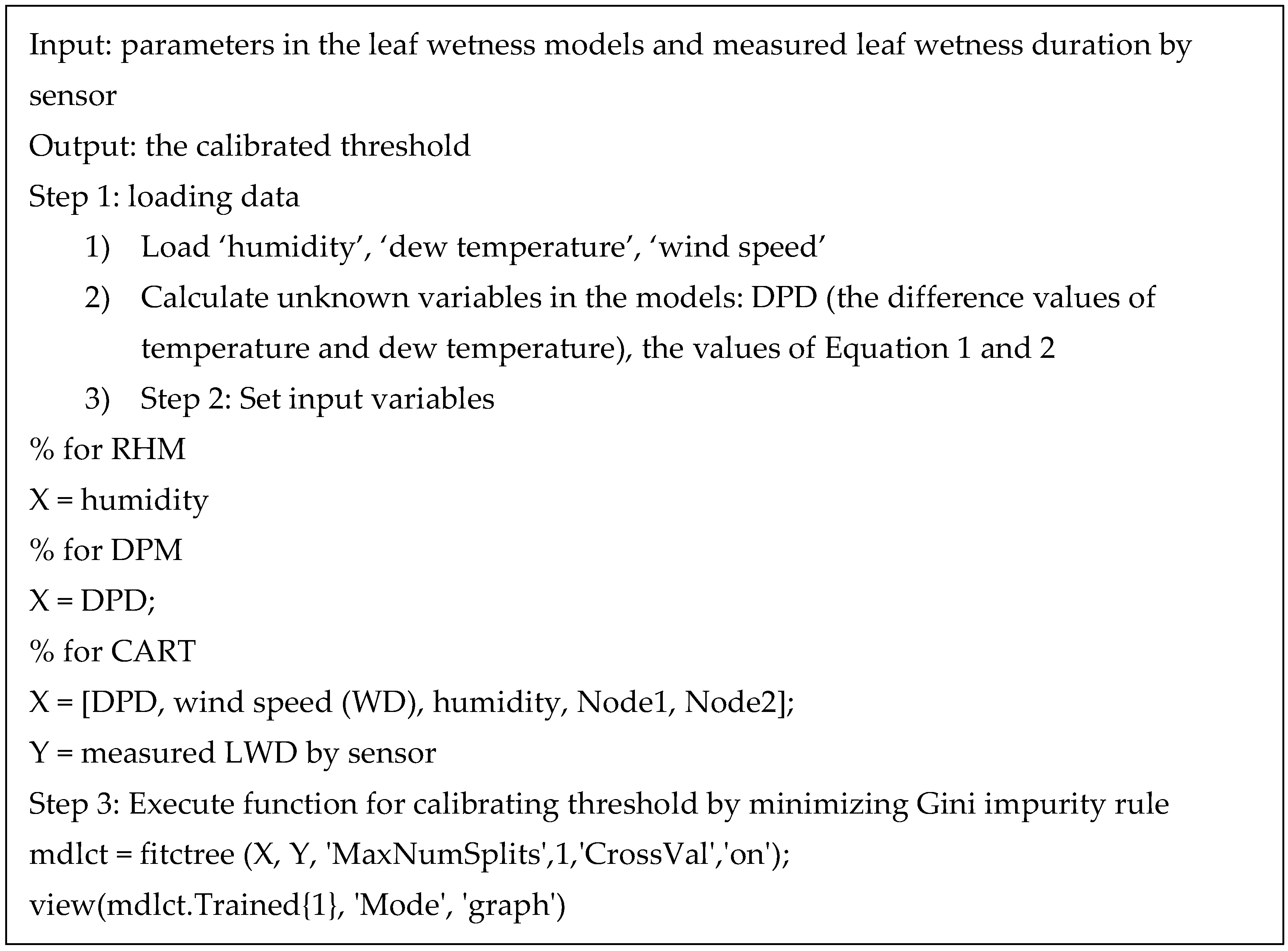
A decision learning tree is a commonly used method in data mining and classification [35]. A decision tree algorithm works by splitting a dataset so as to train a model through a recursive partitioning process. Then the model is used to predict the value of a target variable based on the independent variables (Figure 6). In the leaf wetness models, the model parameters are independent variables (X) while leaf wetness is the classification variable (wet = 1, dry = 0). The splitting rule is that a sample goes right if a ‘feature value X ≤ C′, otherwise it goes left. The Gini index is the criterion used to reduce the impurity in classification splitting since it can be computed more rapidly and be readily extended to include symmetrized costs [26]. The Gini index of node impurity in the leaf wetness classification problem can be expressed as in Equation (3). The Gini index reaches a zero value when only one class is present at a node. This means that the Gini index will be zero if all cases at a node belong to the same class, where p(t) denotes the relative frequency of the first class at the node. The process of calibrating the leaf wetness models (RHM, DPM and CART) thresholds by the decision learning tree method using the MATLAB tool is shown in Figure 7.

$$\mathrm{G}\left(\mathrm{t}\right)=1-\mathrm{p}{\left(\mathrm{t}\right)}^2-{\left(1-\mathrm{p}\left(\mathrm{t}\right)\right)}^2$$

(3)

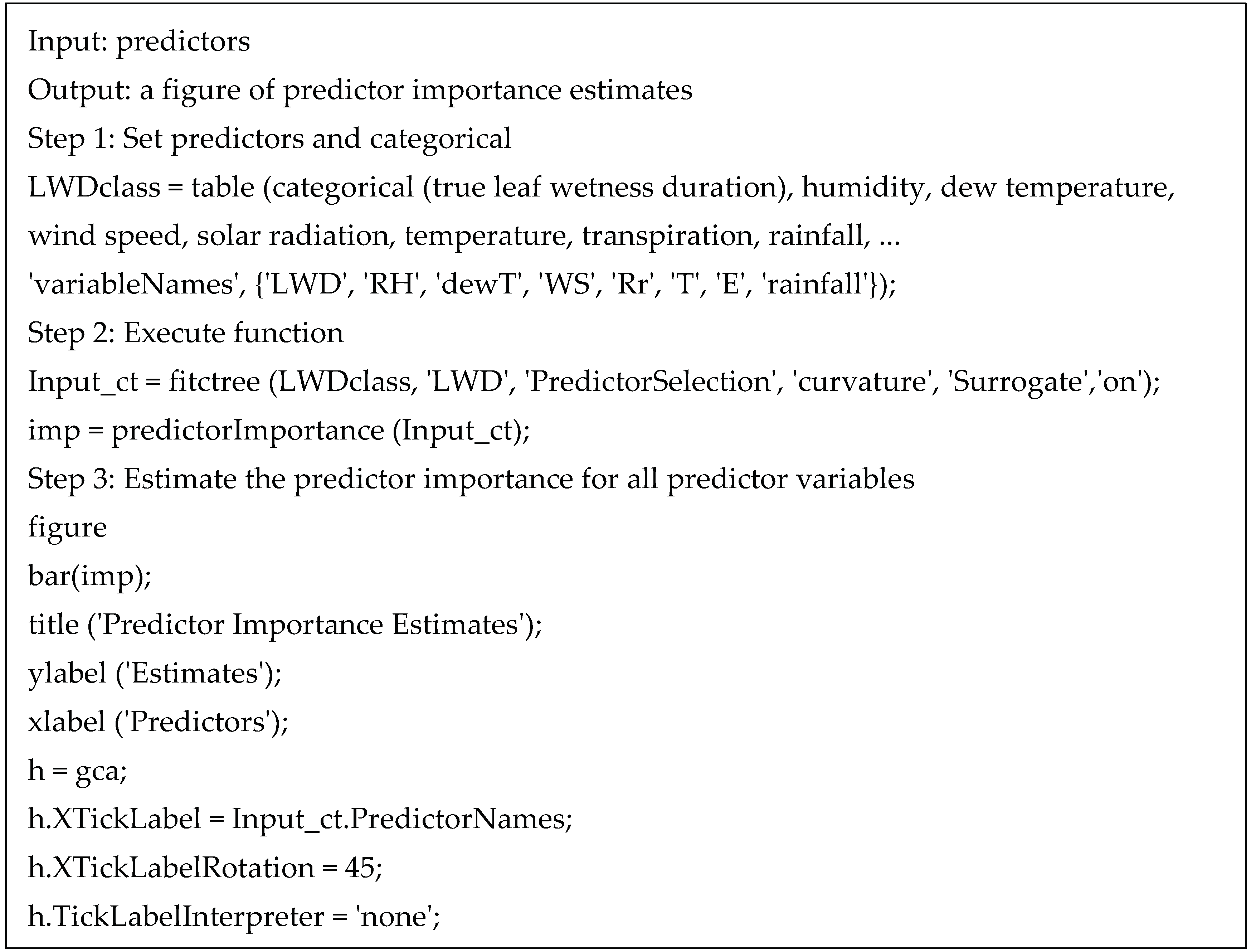
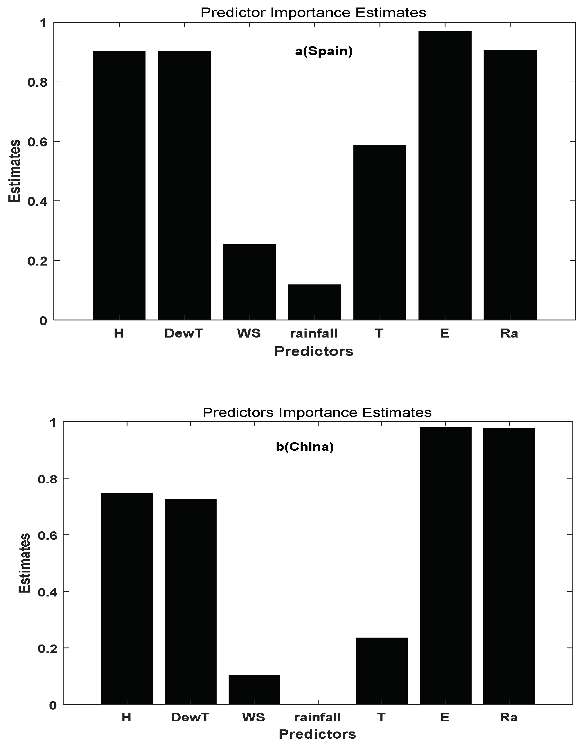
Usually, input parameters are chosen based on expertise and historical data [25]. In this article, by employing the decision tree method it has been possible to use a predictor importance ranking to help select the most effective factors and reduce time lost; the process is shown in Figure 8. The predictor’s importance is computed by totaling the changes in the mean squared error (MSE) caused by the splits for each predictor, and then dividing the total by the number of branch nodes. The variable importance associated with this split is computed as the difference between MSE for the parent node and the total MSE for the two child nodes. In our case, the predictor’s importance had the same rank for the Spanish (Figure 9a) and Chinese greenhouses (Figure 9b). Relative humidity (RH), dew temperature (dewT), transpiration (E) and radiation (Ra) were the first four predictors ranked in importance for LWD.

Analyzing sensitivity of the NNM to individual inputs aims to evaluate the feasibility of simplifying the number of NNM inputs (

Table 3. Sensitivity of artificial neural network models of wetness status at the tomato leaf level to different input variables.

Inputs/Locations	Accuracy on Test Data		Accuracy on Validation Data
	Spain	China	Spain	China
Relative humidity (H)	0.73	0.83	0.60	0.72
Dew temperature (dewT)	0.73	0.83	0.65	0.71
Transpiration (E)	0.93	0.87	0.70	0.74
Radiation (Ra)	0.85	0.88	0.70	0.74
(H, Ra)	0.88	0.89	0.76	0.78
(H, dewT, E, Ra)	0.82	0.98	0.88	0.92

). When humidity and radiation were the inputs of the NNM, the model had higher accuracy than the model with individual inputs. It was better to use the NNM with the four inputs in our case, because of its highest accuracy of 0.88 for Spain and 0.92 for China. Therefore, the group of four parameters—relative humidity, dew temperature, transpiration and radiation—made up the new NNM input parameters (Figure 10). Transpiration was estimated using a referenced method [18].

2.4. Evaluation Criteria

In general, higher values of the positive predictive value (PPV), negative predictive value (NPV), sensitivity (Sen) and accuracy (Acc) resulted in better model performance [36]. The EF indicates how well the relationship between the observed and simulated data fit with regard to the 1:1 straight line, with the optimum EF value = 1.0. For a perfect classifier, the area under the receiver operating characteristic curve (AUC) = 1, where t is the threshold parameter, Pt is the true positive value number, Pf is the false positive value number, Nf is the false negative value number, and Nt is the true negative value number. E_i is the ith value of estimated leaf wetness, A_i is the ith value of true leaf wetness, A_meani is the mean value of true leaf wetness, and N is the sample size. These indexes were computed by Equations (4)–(9). Two error analyses of mean absolute error (MAE) and standard deviation (SD) also were used to assess the models’ behavior by comparing estimated and measured LWD (Equations (10) and (11)).

$$\mathrm{PPV}=\frac{Pt}{Pf+Pt}$$

(4)

$$\mathrm{NPV}=\frac{Nt}{Nf+Nt}$$

(5)

$$\mathrm{Sen}=\frac{Pt}{Pt+Nf}$$

(6)

$$\mathrm{Acc}=\frac{Pt+Nt}{Pf+Pt+Nf+Nt}$$

(7)

$$\mathrm{AUC}={{\displaystyle \int }}_{\infty }^{-\infty }PPV\left(t\right)\left(-\acute{NPV\left(t\right)}\right)dt$$

(8)

$$\mathrm{EF}=\frac{{{\displaystyle \sum }}_{i=1}^N{\left(A_i-E_i\right)}^2}{{{\displaystyle \sum }}_{i=1}^N{\left(A_i-Amean\right)}^2}$$

(9)

$$\mathrm{MAE}=\frac{{{\displaystyle \sum }}_{i=1}^N\left|A_i-E_i\right|}{N}$$

(10)

$$\mathrm{SD}=\sqrt{\frac{{{\displaystyle \sum }}_{i=1}^N{\left(A_i-E_i\right)}^2}{N}}$$

(11)

3. Results

The calibration dataset included data collected in the Spanish greenhouse (ES) from April 2016 to December 2016 and in the Chinese greenhouse (CN) from April 2014 to November 2014 (Figure 11, Figure 12, Figure 13 and Figure 14). The model evaluation was performed using ES data in the period March 2017 to February 2018 and CN data from December 2014 to September 2015 (Figure 15). The statistical indices used to evaluate leaf wetness model performance were taken from Gil et al. [22] and Tien et al. [37], and are listed in Equations (4)–(11).

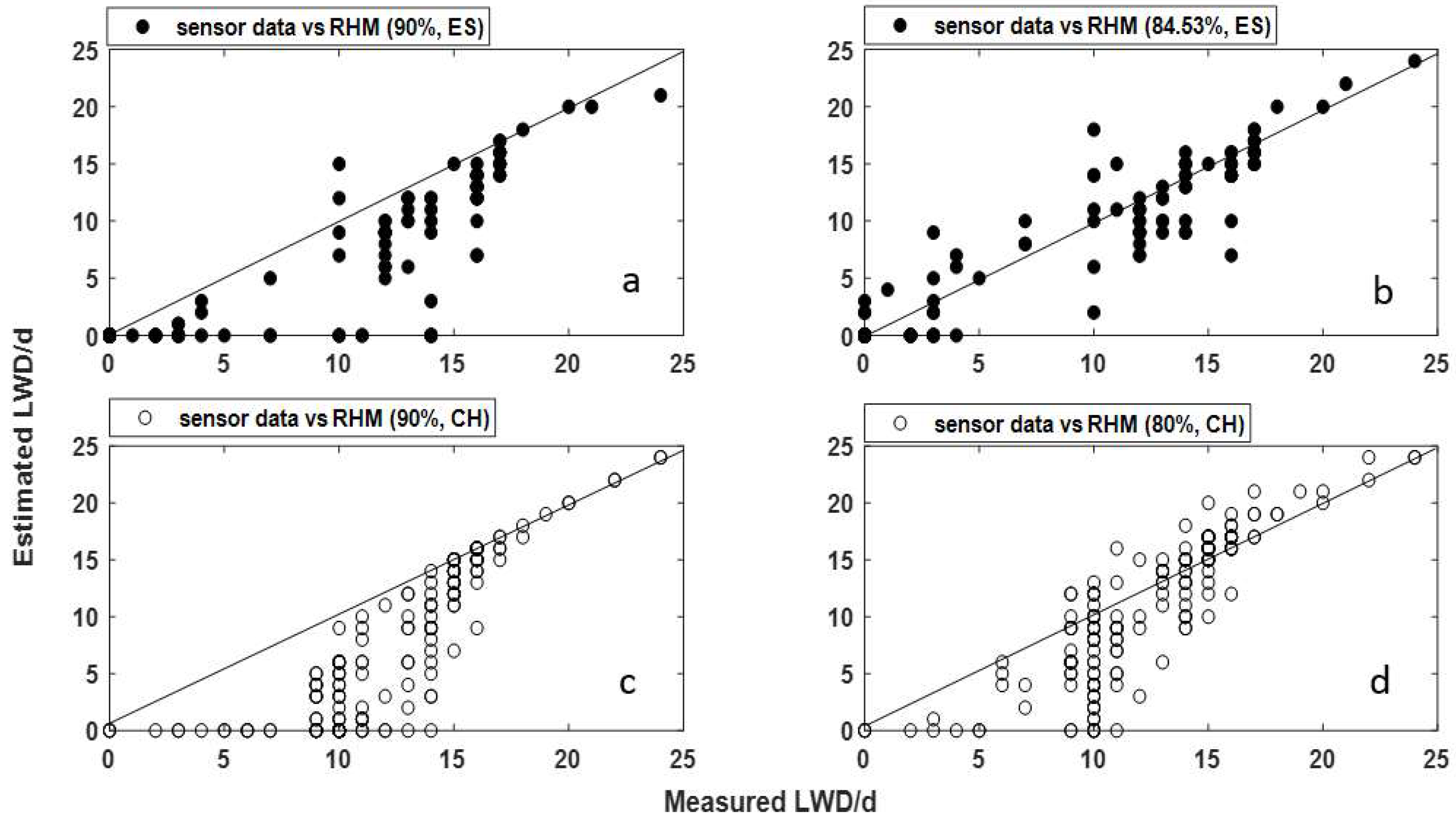
Four scatter plots between estimated and measured LWD using RHM in the two greenhouses are shown in Figure 11. When the empirical threshold (RH > 90%) was used, the data deviated from the 1:1 straight line (Figure 11a,c); on the contrary, the model performance improved when the threshold was calibrated to 84.53% in the ES greenhouse and 80% in the CN greenhouse, with an EF of 0.95 (ES) and 0.97 (CN). In particular, the accuracy of the model greatly improved, with a Sen of 0.53 (ES) and 0.85 (CN), while PPV and NPV also increased, with an Acc of 0.83 (ES) and 0.80 (CN). After calibration, the mean absolute error decreased from 7.12 h to 5.31 h in ES and from 6.12 h to 2.73 h in CN (

Table 4. Performance statistic values of the relative humidity model (RHM) of the two greenhouses, including positive predictive value (PPV), negative predictive value (NPV), sensitivity (Sen), accuracy (Acc), area under receiver operating characteristic curve (AUC), effective fitting (EF), mean absolute error (MAE) and standard deviation (SD).

Location.	RHM	PPV	NPV	Sen	Acc	AUC	EF	MAE (h)	SD (h)
Spain	Experiential threshold (RH > 90%)	0.63	0.82	0.30	0.80	0.83	1.14	7.12	8.12
	Calibrated threshold (RH > 84.53%)	0.67	0.87	0.53	0.83	0.84	0.95	5.31	6.42
China	Experiential threshold (RH > 90%)	0.55	0.89	0.39	0.78	0.83	0.79	6.12	7.45
	Calibrated threshold (RH > 80%)	0.77	0.84	0.85	0.80	0.82	0.97	2.73	3.81

).

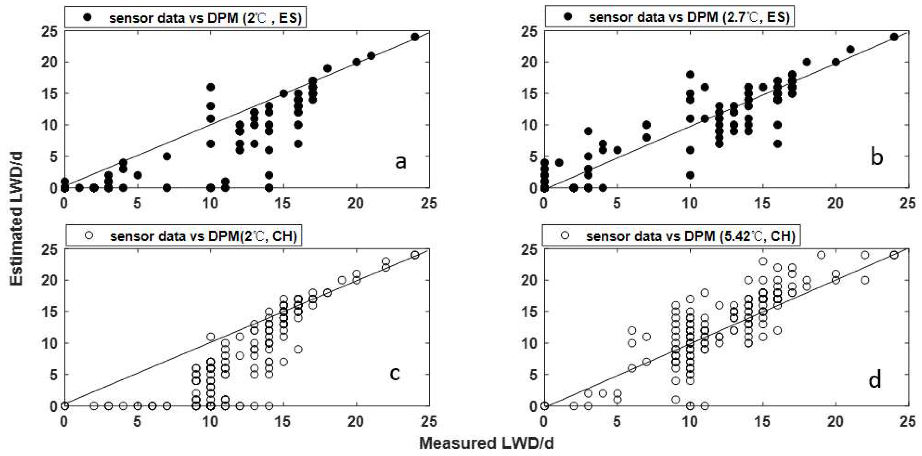
The differences in the performance of the DPM before (DPD < 2 °C) and after calibration (DPD < 2.7 °C for ES and DPD < 5.42 °C for CN) could be explained by the data distribution in the scatter plots (Figure 12) and the performance statistic values in

Table 5. Performance statistic values of the dew temperature model (DPM) of the two greenhouses, including positive predictive value (PPV), negative predictive value (NPV), sensitivity (Sen), accuracy (Acc), area under receiver operating characteristic curve (AUC), effective fitting (EF), mean absolute error (MAE) and standard deviation (SD).

Location	DPM	PPV	NPV	Sen	Acc	AUC	EF	MAE (h)	SD (h)
Spain	Experiential threshold (DPD < 2 °C)	0.64	0.83	0.38	0.81	0.84	1.08	7.84	8.87
	Calibrated threshold (DPD < 2.7 °C)	0.67	0.87	0.56	0.83	0.85	0.94	5.16	6.33
China	Experiential threshold (DPD < 2 °C)	0.59	0.87	0.41	0.77	0.81	0.81	4.55	5.93
	Calibrated threshold (DPD < 5.42 °C)	0.79	0.81	0.83	0.80	0.82	0.93	2.30	3.04

. The calibrated DPM threshold reduced the estimation of LWD, as proved by data distributions shown in Figure 12b,d, which fitted better to the 1:1 straight line than in Figure 12a,c. Moreover, the PPV increased to 0.67 (ES) and 0.79 (CN), Sen rose to 0.56 (ES) and 0.83 (CN), and Acc reached 0.83 (ES) and 0.80 (CN). The effectiveness of the calibration threshold was also proved by lower MAE and SD than with the DPD threshold fixed at 2 °C (Table 5).

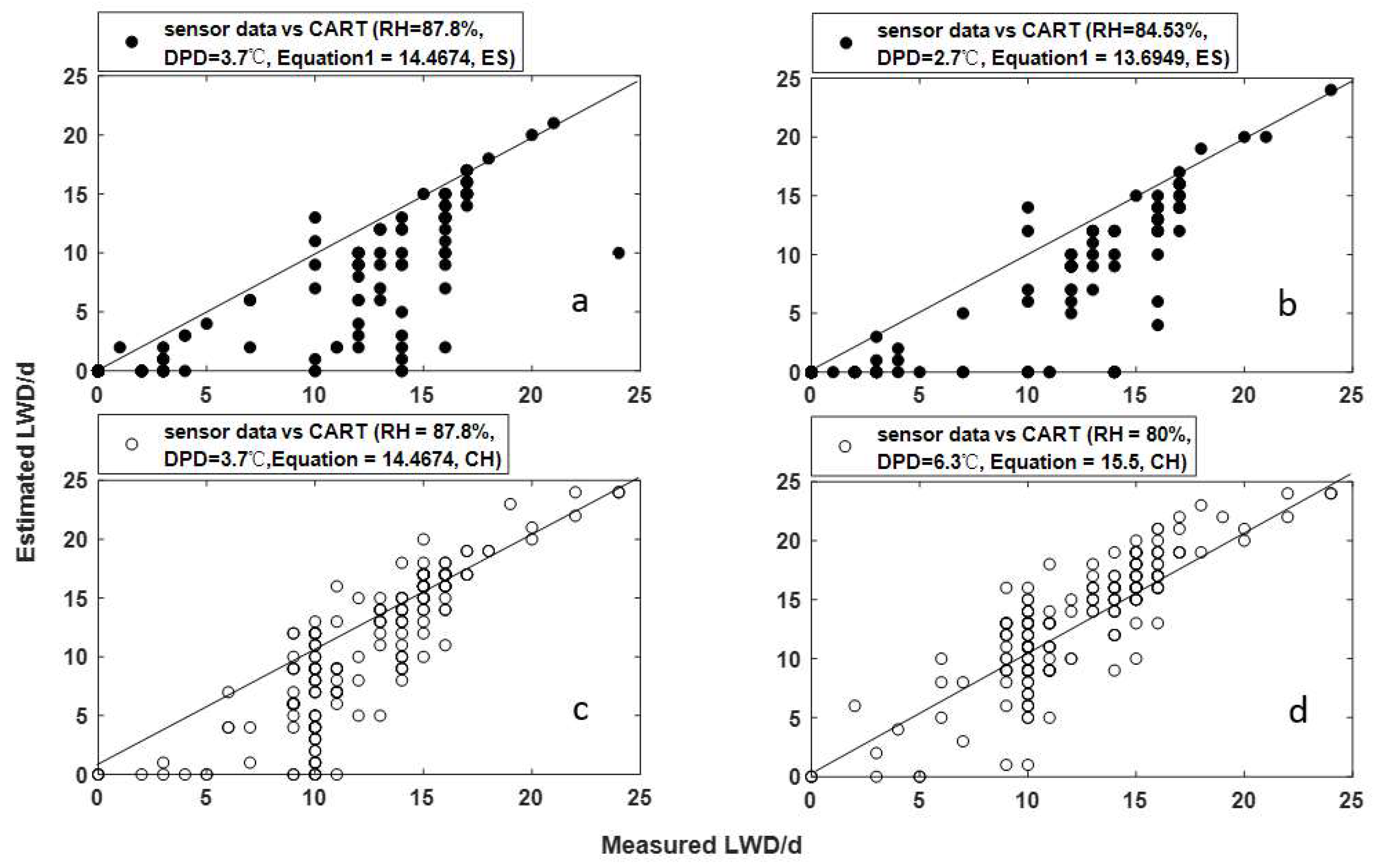
The calibration CART model maintained the four categories, but with different thresholds. The first category is to identify whether the leaf is wet or dry depending on the DPD value. The original threshold (3.7 °C) was modified to 2.7 °C for ES and 6.3 °C for CN. Equation (1) was applied to evaluate leaf wetness occurrence in conditions of low wind speed (wind speed < 2.5 m s⁻¹), whereas Equation (2) was used when RH is high (relative humidity above 87.8%). This work kept these coefficients in Equation (1) unchanged, to limit the calibration of the CART model to the thresholds leading to new node splitting (13.6949 for Spain, 15.5 for China), while adopting the conditions of relative humidity greater than 84.53% for Spain and 80% for China before using Equation (2) to identify leaf class (Figure 13). The model performance showed great improvement, which can be proved by comparing statistic values that were calculated before and after calibration of the model, with an AUC of 0.88 (in ES) and 0.91 (in CN), as well as an Acc of 0.83 (in ES) and 0.82 (in CN). The better performance of the calibrated model also was reflected in lower MAE and SD, which were 4.60 h and 5.92 h for ES, and 2.13 h and 2.84 h for CN, respectively (

Table 6. Performance statistic values of the classification and regression tree model with experiential and calibrated threshold.

Location	CART	PPV	NPV	Sen	Acc	AUC	EF	MAE (h)	SD (h)
Spain	Experiential threshold (RH < 87.8%, DPD < 3.7 °C, Equation (1) > 14.4674)	0.63	0.83	0.36	0.80	0.84	1.11	6.19	7.38
	Calibrated threshold (RH < 84.53%, DPD < 2.7 °C, Equation (1) > 13.6949)	0.63	0.89	0.62	0.83	0.88	0.96	4.60	5.29
China	Experiential threshold (RH < 87.8%, DPD < 3.7 °C, Equation (1) > 14.4674)	0.73	0.88	0.49	0.80	0.78	0.82	3.18	4.49
	Calibrated threshold (RH < 80%, DPD < 6.3 °C, Equation (1) > 15.5)	0.83	0.80	0.83	0.82	0.91	1.09	2.13	2.84

).

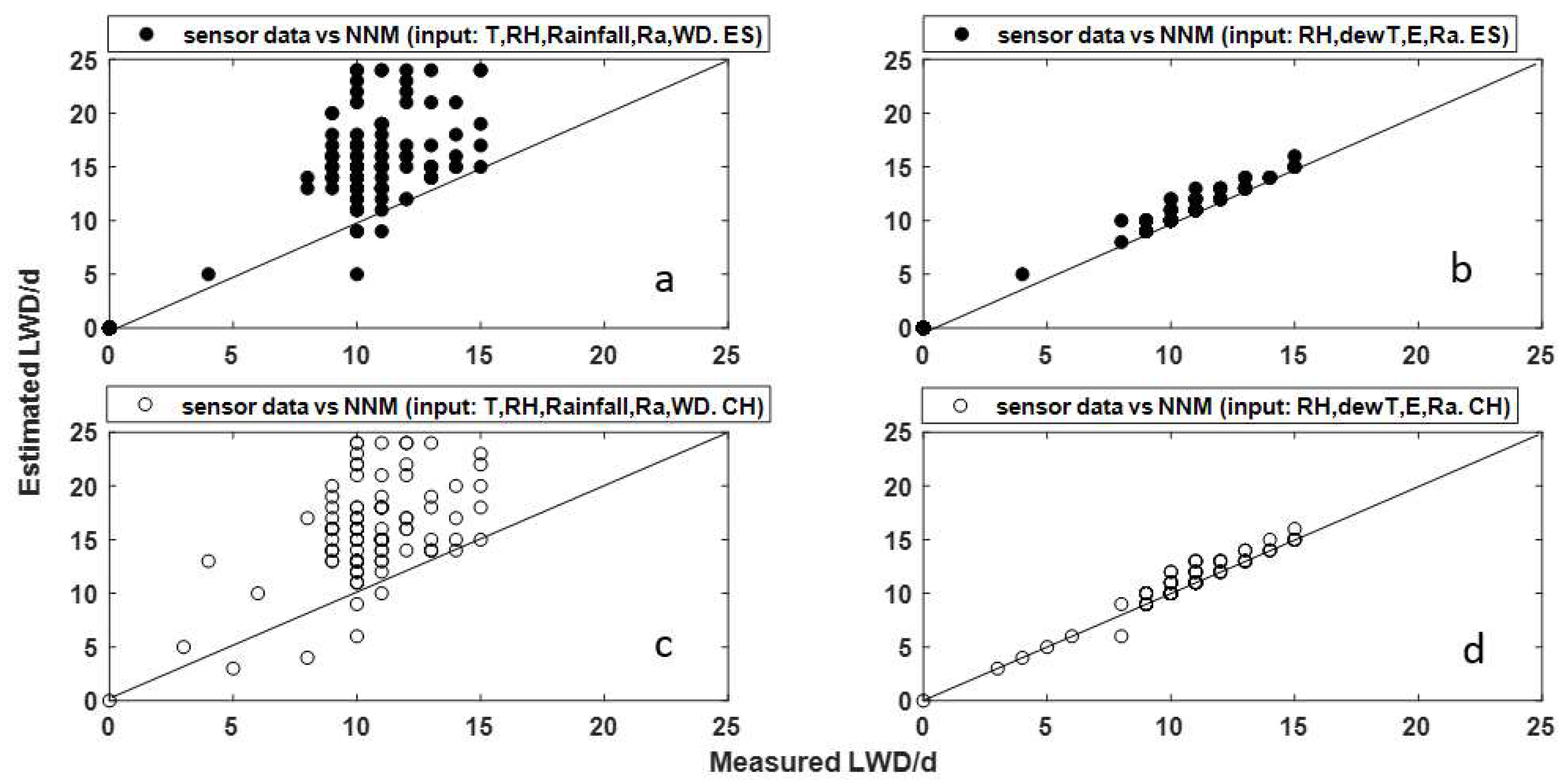
The results of estimation of LWD by the NNM with new input parameters are quite different from the results obtained from the NNM with empirical inputs. More importantly, the importance of the new input parameters was reflected in the good fitting result of LWD estimation to the 1:1 straight line (Figure 14b,d), with an EF of 1.05 (ES) and 0.97 (CN). This model is a good classifier, with an AUC of 0.88 (ES) and 0.97 (CN). Furthermore, the NNM with new input parameters has lower error of estimation of LWD (

Table 7. Performance statistic values of the neural network model (NNM) of two greenhouses, including positive predictive value (PPV), negative predictive value (NPV), sensitivity (Sen), accuracy (Acc), area under receiver operating characteristic curve (AUC), effective fitting (EF), mean absolute error (MAE) and standard deviation (SD).

Location	NNM	PPV	NPV	Sen	Acc	AUC	EF	MAE (h)	SD (h)
Spain	Experiential Inputes (T, RH, Rainfall, Ra, WD)	0.92	0.68	0.56	0.75	0.87	1.36	5.10	6.25
	Calibrated Inputes (RH, dewT, E, Ra)	0.92	0.77	0.64	0.82	0.88	1.05	0.23	0.65
China	Experiential Inputes (T, RH, Rainfall, Ra, WD)	0.89	0.54	0.62	0.70	0.75	1.09	5.38	6.57
	Calibrated Inputes (RH, dewT, E, Ra)	0.99	0.88	0.88	0.98	0.97	0.97	0.34	0.67

), with a MAE of 0.23 h (ES) and 0.34 h (CN), and an SD of 0.65 h (ES) and 0.67 h (CN).

The evaluation data were acquired in Spain from March 2017 to February 2018 and in China from December 2014 to October 2015. These data were used to assess the calibration models’ performance. Comparison results of estimated and measured LWD are shown in Figure 15. Most subfigures in Figure 15 show a good fitting, however, large errors remained, even after calibration (Figure 15, RHM-ES). A multi-model comparison was carried out to rank model performances (

Table 8. Performance statistic values of the LWD models in two greenhouses: relative humidity model (RHM), dew temperature model (DPM) and neural network model (NNM).

Location	Spain				China
Index/Mode	RHM	DPM	CART	NNM	RHM	DPM	CART	NNM
PPV	0.71	0.71	0.77	0.82	0.85	0.86	0.84	0.90
NPV	0.72	0.71	0.76	0.87	0.80	0.78	0.87	0.92
Sen	0.62	0.64	0.68	0.85	0.75	0.80	0.81	0.89
Acc	0.73	0.73	0.76	0.88	0.87	0.86	0.86	0.92
AUC	0.73	0.74	0.77	0.90	0.79	0.83	0.84	0.94
EF	0.83	0.83	0.85	0.92	0.85	0.86	0.88	0.94
MAE	5.45	5.46	3.46	1.85	3.42	3.29	2.75	1.30
SD	6.11	6.11	4.11	2.25	4.43	4.20	3.51	1.62

Note: performance statistics indices include: positive predictive value (PPV), negative predictive value (NPV), sensitivity (Sen), accuracy (Acc), the area under receiver operating characteristic curve (AUC), EF (effective fitting), mean absolute error (MAE) and root mean square error (RMSE).

). The NNM was the most efficient at estimating LWD in ES, with a PPV of 0.82 and a NPV of 0.87, while also it has higher accuracy, with 1.85 h (MAE) and 2.25 h (SD). Furthermore, the results of estimation of LWD of the other LWD models were similar, with low ranges of PPV [0.71 0.77], and NPV [0.71 0.76]. For the Chinese greenhouse, the NNM obtained an excellent result of LWD estimation, with a PPV of 0.90, a NPV of 0.92, a MAE of 1.30 h and a SD of 1.62 h.

4. Discussion

The results confirmed that a site-specific calibration was needed to improve leaf wetness model accuracy, in agreement with literature studies. Gil et al. adopted the calibrated threshold for the RHM (RH > 94%) and for the DPM (DPD < 2 °C), which were used for LWD estimation in Colombia, and the correct success index of the models were 0.69 and 0.65, respectively [22]. Bassimba et al. [14] calibrated the threshold of the RHM for 14 commercial citrus orchards in Spain by ROC curve analysis, and sensibility of the model was in the range of 0.43–0.93. Mashonjowa et al. [12] proposed the calibration thresholds of the RHM (RH > 84%) and the DPM (DPD < 2.5 °C) for a Zimbabwe greenhouse, and the correct success index of each model was 0.59 and 0.76. Empirical leaf wetness models after calibration of thresholds, such as the RHM and DPM, did not perform better than the complex physical models. Sentelhas et al. [8] obtained a mean absolute error of around 1.6 h with a Penman–Monteith-based approach. Dalla Marta et al. [38] found the mean absolute errors of the physical model were between 1.5 h and 2.3 h. In this study, the mean absolute errors of estimation of LWD of RHM were in the range of 3.29–5.46 h for the test locations (Table 8), but the CART model achieved a similar performance: the MAE of this model was 2.75 h for China and 3.46 h for Spain. Although the CART model used different meteorological inputs, the implicit representation of the physical principles leading to leaf wetness provides some spatial portability for the CART model. Nonetheless, we recommend a specific calibration to adapt the model to new greenhouse systems because of the good results of estimation of LWD demonstrated at this point (Table 6).

Neural networks can be used for estimating LWD, even though they do not provide an explicit formalization of the relationship between leaf wetness duration and climate data, which could vary even within a greenhouse system. If the choice of the predictors is inaccurate, this typology of model might lead to significant errors, as in our study without specific calibration (5.10 h for China and 5.38 h for Spain). Francl et al. [24] analyzed sensitivity of an artificial neural network model of wet status at the wheat flag leaf level to individual input variables, and demonstrated that humidity was the most important factor, followed by temperature and solar radiation. These results are in agreement with our findings. Rainfall and wind speed made a small contribution to model accuracy, which can be proved by the result of predictor importance estimates in Figure 9. This conclusion agreed with Francl et al. [24]. The two parameters were important for estimation of LWD of an open field, as in Stella et al. [25], who evaluated leaf wetness for improving apple scab resistance by an NNM; Dalla Marta et al. [29] estimated leaf wetness duration for simulating Plasmopara viticola infection. In this work, the NNMs obtained good performances with the same inputs in the two locations (Table 8), which were the same as in Francl et al. [24]. This study also indicated that transpiration has the same importance as radiation in estimation of LWD inside a greenhouse. However, transpiration and dew temperature are variables not commonly available in standard weather stations.

This work mainly focusses on an analysis to prove that a decision learning tree can lead to an effective calibration of leaf wetness models, and that this preliminary calibration is needed when applying empirical leaf wetness models in new conditions. Although the plant architecture and its thermal properties are two of the causes of differences of the leaf wetness models, their inclusion in available models is limited to process-based models and semi-empirical approaches; for example, Magarey et al. [9] developed the surface wetness energy balance model to estimate LWD on grape plants, considering the balance between the canopy water budget and the sum of canopy water storage capacity, intercepted rain or irrigation, and the volume of water on the leaf as dew and the volume of water evaporation. Kim et al. also developed a fuzzy logical model based on energy balance principles [39]. Ferentinos et al. [40] analyzed the spatial distribution of temperature, humidity, condensation condition risk and transpiration variability inside a greenhouse; all of these environment parameters has a spatial variation that is due to the measurement error caused by the limitation of the sensors. More importantly, calibration parameters of leaf wetness models are also an important reason for the different results of estimation of LWD for each location because the empirical models rely on local climate data and empirical input conditions. Thus, this work highlights the effectiveness of site-specific thresholds and inputs of leaf wetness models when they are implemented in different systems, proved by comparing model performance before and after calibration.

5. Conclusions

The calibration of leaf wetness model parameters is a main source of variation in LWD estimation in different locations, especially for empirical models which are based on local climatic data and input conditions. This paper emphasizes the analysis of the positive effect of the calibrated thresholds and conditions on leaf wetness model performance by the decision learning tree method in two greenhouse systems, in Spain and China. Accordingly, the parameters of relative humidity, dew temperature, classification and regression tree and neural network models were calibrated using a classification tree. The following conclusions are drawn in this study:

• The calibration of the parameters of leaf wetness models is effective for reducing the error between estimated LWD and measured LWD, and thus has the potential to greatly improve the model accuracy.
• Humidity, dew temperature, transpiration and radiation are the variables mostly contributing to the precision of a neural network model (NNM) for LWD estimation.
• Evaluation results showed that NNM was the most accurate in estimating LWD both in Spanish and Chinese greenhouses, with low error between estimated and measured LWD. All the other models obtained similar results in the two tested conditions.

References

- Magarey, R.D.; Russo, J.M.; Seem, R.C.; Gadoury, D.M. Surface wetness duration under controlled environmental conditions. Agric. For. Meteorol. 2005, 128, 111–122. [Google Scholar] [CrossRef]
- Emilio, M.; Franco, E.; Troncozo, M.I.; Marianela, S.; López, Y.; Lucentini, G.; Medina, R.; Carlos, M.; Saparrat, N.; Ronco, L.B.; et al. A survey on tomato leaf grey spot in the two main production areas of Argentina led to the isolation of Stemphylium lycopersici representatives which were genetically diverse and differed in their virulence. Eur. J. Plant Pathol 2017, 149, 983–1000. [Google Scholar] [CrossRef]
- Ward, J.M.; Stromberg, E.L.; Nowell, D.C.; Nutter Jr, F.W. Gray leaf spot: a disease of global importance in maize production. Plant Dis. 1999, 83, 884–895. [Google Scholar] [CrossRef]
- Huber, L.; Gillespie, T.J. Modeling leaf wetness in relation to plant disease epidemiology. Ann. Rev. Phytopathol 1992, 30, 553–577. [Google Scholar] [CrossRef]
- Magarey, R.D.; Sutton, T.B.; Thayer, C.L. A Simple Generic Infection Model for Foliar Fungal Plant Pathogens. Phytopathology 2005, 95, 92–100. [Google Scholar] [CrossRef] [PubMed]
- Rodríguez, F.; Berenguel, M.; Guzmán, J.L.; Ramírez-Arias, A. Modeling and Control of Greenhouse Crop Growth; Springer: London, UK, 2015; ISBN 978-3-319-11133-9. [Google Scholar]
- Sánchez-Molina, J.A.; Rodríguez, F.; Guzmán, J.L.; Arahal, M.R. Virtual sensors for designing irrigation controllers in greenhouses. Sensors 2012, 12, 15244–15266. [Google Scholar] [CrossRef]
- Sentelhas, P.C.; Gillespie, T.J.; Santos, E.A. Evaluation of FAO Penman–Monteith and alternative methods for estimating reference evapotranspiration with missing data in Southern Ontario, Canada. Agric. Water Manag. 2010, 97, 635–644. [Google Scholar] [CrossRef]
- Magarey, R.D.; Russo, J.M.; Seem, R.C. Simulation of surface wetness with a water budget and energy balance approach. Agric. For. Meteorol. 2006, 139, 373–381. [Google Scholar] [CrossRef]
- Bregaglio, S.; Frasso, N.; Pagani, V.; Stella, T.; Francone, C.; Cappelli, G.; Acutis, M.; Balaghi, R.; Ouabbou, H.; Paleari, L.; et al. New multi-model approach gives good estimations of wheat yield under semi-arid climate in Morocco. Agron. Sustain. Dev. 2015, 35, 157–167. [Google Scholar] [CrossRef]
- Zhao, C.J.; Li, M.; Yang, X.T.; Sun, C.H.; Qian, J.P.; Ji, Z.T. A data-driven model simulating primary infection probabilities of cucumber downy mildew for use in early warning systems in solar greenhouses. Comput. Electron. Agric. 2011, 76, 306–315. [Google Scholar] [CrossRef]
- Mashonjowa, E.; Ronsse, F.; Mubvumac, M.; Milford, J.R.; Pieters, J.G. Estimation of leaf wetness duration for greenhouse roses using a dynamic greenhouse climate model in Zimbabwe. Comput. Electron. Agric. 2013, 95, 70–81. [Google Scholar] [CrossRef]
- Sentelhas, P.C.; Dalla Marta, A.; Orlandini, S.; Santos, E.A.; Gillespie, T.J.; Gleason, M.L. Suitability of relative humidity as an estimator of leaf wetness duration. Agric. For. Meteorol. 2008, 148, 392–400. [Google Scholar] [CrossRef]
- Bassimba, D.D.M.; Intrigliolo, D.S.; Dalla Marta, A.; Orlandini, S.; Vicent, A. Leaf wetness duration in irrigated citrus orchards in the Mediterranean climate conditions. Agric. For. Meteorol. 2017, 234, 182–195. [Google Scholar] [CrossRef]
- Kim, K.S.; Taylor, S.E.; Gleason, M.L.; Villalobos, R.; Arauz, L.F. Estimation of leaf wetness duration using empirical models in northwestern Costa Rica. Agric. For. Meteorol. 2005, 129, 53–67. [Google Scholar] [CrossRef]
- Gillespie, T.J.; Srivastava, B.; Pitblado, R.E. Using operational weather data to schedule fungicide sprays on tomatoes in southern Ontario, Canada. J. Appl. Meteorol. 1993, 32, 567–573. [Google Scholar] [CrossRef]
- Nury, A.H.; Hasan, K.; Alam, M.J.B. Comparative study of wavelet-ARIMA and wavelet-ANN models for temperature time series data in northeastern Bangladesh. J. King Saud Univ. 2017, 29, 47–61. [Google Scholar] [CrossRef] [Green Version]
- Wang, H.; Sánchez-Molina, J.A.; Li, M.; Berenguel, M.; Yang, X.T.; Bienvenido, J.F. Leaf area index estimation for a greenhouse transpiration model using external climate conditions based on genetics algorithms, back-propagation neural networks and nonlinear autoregressive exogenous models. Agric. Water Manag. 2017, 183, 107–115. [Google Scholar] [CrossRef]
- Paul, P.A.; Munkvold, G.P. Regression and artificial neural network modeling for the prediction of gray leaf spot of maize. Phytopathology 2005, 95, 388–396. [Google Scholar] [CrossRef]
- Tsakiri, K.; Marsellos, A.; Kapetanakis, S. Artificial Neural Network and Multiple Linear Regression for Flood Prediction in Mohawk River, New York. Water 2018, 10, 1158. [Google Scholar] [CrossRef]
- Mackenzie, S.J.; Peres, N.A. Use of Leaf Wetness and Temperature to Time Fungicide Applications to Control Anthracnose Fruit Rot of Strawberry in Florida. Plant Dis. 2012, 96, 529–536. [Google Scholar] [CrossRef]
- Gil, R.; Bojacá, C.R.; Schrevensc, E. Suitability evaluation of four methods to estimate leaf wetness duration in a greenhouse rose crop. Acta Hortic. 2011, 893, 797–804. [Google Scholar] [CrossRef]
- Braun, M.T.; Oswald, F.L. Exploratory regression analysis: A tool for selecting models and determining predictor importance. Behav. Res. Methods 2011, 43, 331–339. [Google Scholar] [CrossRef] [PubMed]
- Francl, L.J.; Panigrahi, S. Artificial neural network models of wheat leaf wetness. Agric. For. Meteorol. 1997, 88, 57–65. [Google Scholar] [CrossRef]
- Stella, A.; Caliendo, G.; Melgani, F.; Goller, R.; Barazzuol, M.; La Porta, N. Leaf Wetness Evaluation Using Artificial Neural Network for Improving Apple Scab Fight. Environments 2017, 4, 42. [Google Scholar] [CrossRef]
- Wu, X.; Kumar, V.; Quinlan, J.; Ghosh, J.; Yang, Q.; Motoda, H.; McLachlan, G.J.; Ng, A.; Liu, B.; Yu, P.S.; et al. Top 10 algorithms in data mining. Knowl. Inf. Syst. 2008, 14, 1–37. [Google Scholar] [CrossRef]
- Su, J.; Zhang, H. A Fast Decision Tree Learning Algorithm. In Proceedings of the 21st National Conference on Artificial Intelligence, Boston, MA, USA, 16–20 July 2006; Volume 1, pp. 500–505. [Google Scholar]
- Li, M. Early Warning Method and System for Cucumber downy Mildew (Pseudoperonospora cubensis) in Solar Greenhouse. Ph.D. Thesis, China Agriculture University, Beijing, China, 2010. [Google Scholar]
- Marta, A.D.; De Vincenzi, M.; Dietrich, S.; Orlandini, S. Neural network for the estimation of leaf wetness duration: application to a Plasmopara viticola infection forecasting. Phys. Chem. Earth, Parts A/B/C 2005, 30, 91–96. [Google Scholar] [CrossRef]
- Montone, V.O.; Fraisse, C.W.; Peres, N.A.; Sentelhas, P.C.; Gleason, M.; Ellis, M.; Schnabel, G. Evaluation of leaf wetness duration models for operational use in strawberry disease-warning systems in four US states. Int. J. Biometeorol. 2016, 60, 1761–1774. [Google Scholar] [CrossRef] [PubMed]
- Wilks, D.S.; Shen, K.W. Threshold relative humidity duration forecasts for plant disease prediction. J. Appl. Meteorol. 1991, 30, 463–477. [Google Scholar] [CrossRef]
- Rao, P.S.; Gillespie, T.J.; Schaafsma, A.W. Estimating wetness duration on maize ears from meteorological observations. Can. J. soil Sci. 1998, 78, 149–154. [Google Scholar] [CrossRef] [Green Version]
- Gleasom, M.L.; Taylor, S.E.; Loughin, T.M.; Koehler, K.J. Development and validation of an empirical model to estimate the duration of dew periods. Plant Dis. 1994, 78, 1011–1016. [Google Scholar]
- Beucher, A.; Møller, A.B.; Greve, M.H. Artificial neural networks and decision tree classification for predicting soil drainage classes in Denmark. Geoderma 2017. [Google Scholar] [CrossRef]
- Breiman, L.; Friedman, J.; Stone, C.J.; Olshen, R.A. Classification and Regression Trees; CRC press: Boca Raton, FL, USA, 1984. [Google Scholar]
- Pham, B.T.; Pradhan, B.; Bui, D.T.; Prakash, I.; Dholakia, M.B. A comparative study of different machine learning methods for landslide susceptibility assessment: a case study of Uttarakhand area (India). Environ. Model. Softw. 2016, 84, 240–250. [Google Scholar] [CrossRef]
- Tien, D.; Pradhan, B.; Lofman, O.; Revhaug, I. Landslide susceptibility assessment in vietnam using support vector machines, decision tree, and nave bayes models. Math. Probl. Eng. 2012. [Google Scholar] [CrossRef]
- Dalla Marta, A.; Magarey, R.D.; Orlandini, S. Modelling leaf wetness duration and downy mildew simulation on grapevine in Italy. Agric. For. Meteorol. 2005, 132, 84–95. [Google Scholar] [CrossRef]
- Kim, K.S.; Taylor, S.E.; Gleason, M.L. Development and validation of a leaf wetness duration model using a fuzzy logic system. Agric. For. Meteorol. 2004, 127, 53–64. [Google Scholar] [CrossRef]
- Ferentinos, K.P.; Katsoulas, N.; Tzounis, A.; Bartzanas, T.; Kittas, C. Wireless sensor networks for greenhouse climate and plant condition assessment. Biosyst. Eng. 2017, 153, 70–81. [Google Scholar] [CrossRef]
Figure 1.
Schematic of workflow implemented in this paper for calibrating and evaluating leaf wetness models.
Figure 2.
Greenhouse facilities used for the experiments performed in Spain.
Figure 3.
Greenhouse facilities used for the experiments performed in China.
Figure 4.
Schematic diagram of classification and regression tree model (DPD is the difference of air temperature dew temperature (°C), RH is relative humidity (%), WD is the wind speed (m/s))
Figure 5.
Diagram of multiple input and single output neural network modelling.
Figure 6.
Process of optimizing the threshold of a leaf wetness model by decision learning tree.
Figure 7.
Procedure of calibrating leaf wetness models: relative humidity model (RHM), dew temperature model (DPM), and classification and regression tree (CART).
Figure 8.
Procedure of estimating predictor importance.
Figure 9.
A rank of importance of predictor estimates for LWD in the Chinese (a) and Spanish (b) greenhouses.
Figure 10.
Optimized construct of the NNM using decision tree learning.
Figure 11.
Comparison of measured LWD and estimated LWD by the relative humidity model with experiential threshold (90%) and calibrated threshold (84.53% and 80%). ES is the Spanish greenhouse and CN is the Chinese greenhouse.
Figure 12.
Comparison of measured LWD and estimated LWD by the dew temperature model with experiential threshold (2 °C) and calibrated threshold (2.7 °C and 5.42 °C). ES is the Spanish greenhouse, CN is the Chinese greenhouse.
Figure 13.
Comparison of measured LWD and estimated LWD by the classification and regression tree model with experiential threshold and calibrated threshold. ES is the Spanish greenhouse, CN is the Chinese greenhouse.
Figure 14.
Comparison of measured LWD and estimated LWD by the neural network model with the experiential threshold and calibrated threshold.
Figure 15.
Evaluation results of effectiveness of calibrated threshold and conditions on improving leaf wetness models’ behavior in a Spanish greenhouse (ES) and a Chinese greenhouse (CN): relative humidity model (RHM), dew temperature model (DPM) and neural network model (NNM).