Improved Curve Number Estimation in SWAT by Reflecting the Effect of Rainfall Intensity on Runoff Generation

1
College of Computer and Information Engineering, Xiamen University of Technology, Ligong Road 600, Xiamen 361024, China
2
Fujian Engineering and Research Center of Rural Sewage Treatment and Water Safety, Ligong Road 600, Xiamen 361024, China
3
Digital Fujian Institute of Big Data for Natural Hazards Monitor, Ligong Road 600, Xiamen 361024, China
4
Department of Resources and Environmental Sciences, Quanzhou Normal University, Donghai Street 398, Quanzhou 362000, China
5
College of Geographic Sciences, Fujian Normal University, Fuzhou 350007, China
6
Cultivation Base of State Key Laboratory of Humid Subtropical Mountain Ecology, Fujian Normal University, Fuzhou 350007, China
*
Author to whom correspondence should be addressed.
Water 2019, 11(1), 163; https://doi.org/10.3390/w11010163
Submission received: 29 December 2018
/
Revised: 14 January 2019
/
Accepted: 16 January 2019
/
Published: 17 January 2019
(This article belongs to the Section Hydrology)
Abstract
:Determining the amount of rainfall that will eventually become runoff and its pathway is a crucial process in hydrological modelling. We proposed a method to better estimate curve number by adding an additional component (AC) to better account for the effects of daily rainfall intensity on rainfall-runoff generation. This AC is determined by a regression equation developed from the relationship between the AC series derived from fine-tuned calibration processes and observed rainfall series. When incorporated into the Soil and Water Assessment Tool and tested in the Anxi Watershed, it is found, overall, the modified SWAT (SWAT-ICN) outperformed the original SWAT (SWAT-CN) in terms of stream flow, base flow, and annual extreme flow simulation. These models were further evaluated with the data sets of two adjacent watersheds. Similar results were achieved, indicating the ability of the proposed method to better estimate curve number.
1. Introduction
Determining the amount of rainfall that will eventually become runoff (i.e., rainfall-runoff modelling) is a crucial process in hydrological modelling, and there is considerable interest in analysis, comparison, and improvement of the rainfall-runoff models [1,2,3,4,5]. These models do not just predict stream flow amounts at the outlet of a watershed; they also determine whether the water that enters a stream flows over the ground surface or through the soil, and where in the watershed this stream water originates. Thus, rainfall-runoff models that can provide accurate representation of the water flow amounts, pathways, and source areas are key prerequisites for proper water resource management, flood prediction, soil erosion, and non-point source pollution modelling [6,7,8,9,10].
There are two basic kinds of models for surface runoff: physical and empirical models. The physical models, which usually make simplifying assumptions about the runoff generation conditions and have a more rigorous need for driving data (e.g., sub-daily precipitation data), are relatively less used in hydrological modelling than are the empirical models. In contrast, the empirical models, which are based on experience, stem from a tremendous amount of experimental and field work, and are widely used in hydrological modelling. Among these models, the Soil Conservation Service (SCS, currently the Natural Resources Conservation Service) curve number (CN) method, from the mid-1950s, may be the most widely used rainfall-runoff model due to its simplicity, predictability, stability, and lack of serious competition. However, there are some controversies with this method: it is not physically based, it lacks complete historical documentation, and it inadequately represents variable source areas (VSA). It also provides inadequate consideration of the rainfall intensity and duration on runoff generation [2,11,12,13]. Many researchers have proposed adjustments to the CN model to better capture runoff dynamics [8,12,14,15,16,17]. For example, White et al. [15] found that temporal CN adjustments resulted in more accurate simulations, when the CN in the Soil and Water Assessment Tool (SWAT) was changed seasonally to account for variation of watershed storage due to changes in plant growth and dormancy. Zhang et al. [17] also suggested that seasonally adjusted CN could better represent the different runoff generation processes during different periods in the Jinjiang Watershed (southeastern China), which is dominated by a typical subtropical monsoon climate. White el al. [16] proposed a physically based water-balance rainfall-runoff method and incorporated this method into the SWAT model to replace the CN method for estimating runoff generation. They found that the newly modified SWAT (SWAT-WB) significantly improved model predictions in monsoonal climates due to its ability to provide a more realistic distribution of saturated areas (and thus runoff source). The SWAT-WB model was further modified with variable source areas (WB-VSA) by Cheng et al. [12]. The WB-VSA model was compared with four other rainfall-runoff methods (including the soil-water-dependent curve number (CN-Soil), the evaporation-dependent curve number (CN-ET), the G and A equation, and the SWAT-WB) using data from a monsoonal watershed in Eastern China. Their results suggest that the WB-VSA is the most accurate model due to its better reflection of spatial variation of runoff generation, as affected by topography and soil properties.
These studies have better accounted for watershed storage variation and better represented variable source areas to some extent, meanwhile the effect of rainfall intensity on the runoff generation processes are also widely recognized and investigated. Many studies have reported that intense rainfalls are favorable for the formation of a soil skin-crust, which significantly reduces the rate of infiltration. For example, Romkens et al. [18] found that rainfall drops can destroy or deform the arrangement of soil particles and the detached particles can clog the soil pores, thereby reducing the rate of infiltration. Hawke et al. [19] conducted several laboratory experiments to investigate near-surface soil hydrologic conductivity under different rainfall intensities. They found that rainfall intensity had an important influence on the soil hydraulic conductivity. In addition, studies also suggested that intense rainfalls are beneficial to the formation of rills, which facilitate the movement of surface water and therefore increase the surface runoff [20]. Despite that the important impacts of rainfall intensity on soil infiltration and runoff generation have been widely recognized [19,21,22,23,24,25], the effect of rainfall intensity on the CN is seldom investigated and incorporated into hydrological models for practical use. Kim et al. [26] proposed a method uses the temporally weighted average curve number (TWA-CN) by considering the effect of rainfall during a given day as well as the antecedent soil moisture condition to estimate daily surface runoff. It would be still necessary to put more efforts and trials on considering the effect of rainfall intensity on the CN model for better representation of the underlying system in hydrological models.
For this purpose, we proposed a different method from Kim’s method [26] to better estimate curve number by considering the effects of rainfall intensity on rainfall-runoff generation. In this method we introduced an additional component (AC) to existent CN method which account for the effect of rainfall during a given day. Specially, AC is related to rainfall during a given day via regression relationship that was built through a fine-tuned calibration processes. This newly proposed method was incorporated into a SWAT model and tested in the Jinjiang Watershed in southeastern China. Specifically, we first established a hydrological model using SWAT with a data set from the Anxi Watershed (the west branch of the Jinjiang Watershed) and calibrated this model for the interval from January 2000 to December 2006. We then fine-tuned daily CN values by adding an additional component (AC), which was used to account for the effects of rainfall intensity. Next, we developed a regression equation from the additional component and data gathered from a series of observed rainfalls. Finally, we incorporated this regression equation into SWAT and assessed this new version of SWAT (SWAT-ICN) against the original SWAT (SWAT-CN) using data for the Anxi Watershed, and two adjacent watersheds (i.e., Shanmei and Shilong Watersheds, which are the east and downstream branch of the Jinjiang Watershed, respectively) from January 2007 to December 2010.
2. Study Watersheds and Methods
2.1. Study Watersheds
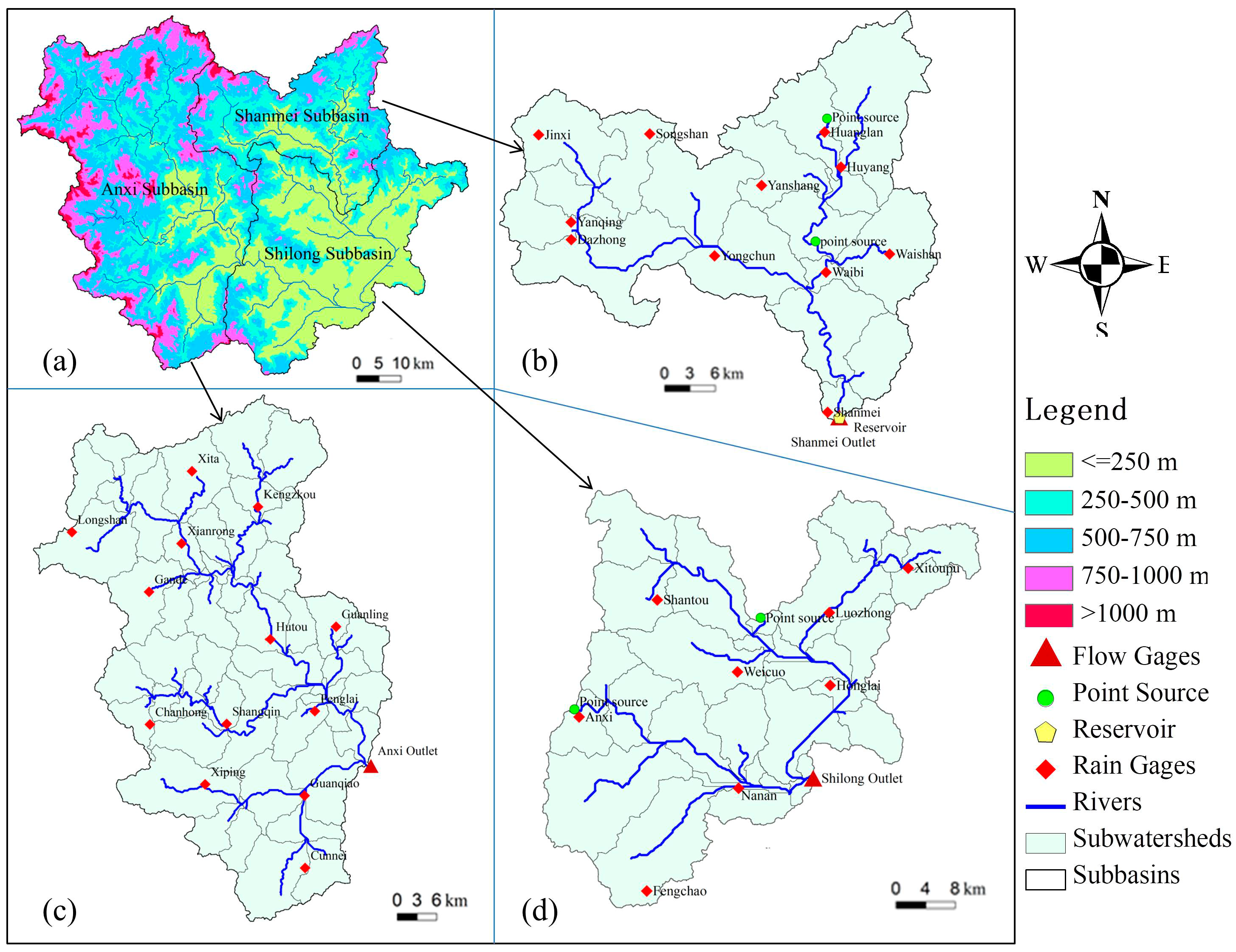
The Jinjiang Watershed is located in southeastern China between 24° 31′ and 25° 32′ N, and 117° 44′ and 118° 47′ E (Figure 1). The drainage area covers 5629 km2, of which approximately 53.8% is located in Quanzhou City. There are two major river branches (east and west) within the Jinjiang Watershed. The length of the total river network and the main section is 302 and 182 km, respectively. There are three hydrological gauge stations: Shanmei, Anxi, and Shilong. The east branch, west branch, and the area downstream from the merge point of the two branches to the watershed outlet, are gauged by the Shanmei, Anxi, and Shilong stations, respectively. Hereafter, these three watersheds are referred to as Shanmei, Anxi, or Shilong Watershed (after the names of the gauge station).
The topography of the study area is dominated by rangelands and mountains, and the major land uses are forest, orchard, cropland, and urbanized area. The soils mainly consist of red soil, yellowish red soil, yellow soil, and paddy soil. The study area is characterized by a subtropical monsoon climate, with an annual mean temperature of 20 °C, ranging from 17 to 21 °C, and with average annual precipitation of 1686 mm (1010–1756 mm). Precipitation events occur mostly during the wet period (May–October), and account for 73% of the annual precipitation. During the wet period, there are flashy convective storms and sea-based typhoons that contribute to approximately 38% of the annual precipitation. During these events, the runoff tends to be generated by infiltration excess due to the high-intensity rainfall. During the dry period (November–April), the runoff is generated mainly by saturation excess processes in saturated or near saturated areas (e.g., riparian zones and wetlands).
2.2. SWAT and SWAT-ICN
SWAT is a quasi-distributed, physical-based hydrologic model developed by the Agricultural Research Service of the US Department of Agriculture to simulate water, sediment, and agricultural chemical transport at river-basin scale [27,28]. As a quasi-distributed hydrologic model, the spatial heterogeneity of the important physical properties of the watershed is delineated by first partitioning a basin or watershed into sub-basins; then further partitioning each sub-basin into hydrologic response units (HRUs) based on the land use, soil types, and topography maps. The HYDROL PROCESS simulated by SWAT can be divided into two major divisions: land phase and routing phase. The land phase first calculates fluxes of water, sediment, nutrients, and pesticides to the main channel in each sub-basin. Major HYDROL PROCESS of this phase include evapotranspiration, canopy storage, infiltration, surface runoff, and sub-surface runoff. The routing phase estimates the movement of such as water and sediment, through the main channel to the sub-basin outlet.
In SWAT, the surface runoff is estimated using either the modified SCS curve number method or the Green and Ampt infiltration method. We focused on the SCS-CN method because daily precipitation data is the only data available currently from the studied watershed. The SCS-CN method was developed to simulate surface runoff from daily rainfall events. It first estimates the amount of overland runoff, and assumes that the remaining precipitation will infiltrate. Overland runoff is defined as:
where Qsurf is the overland runoff or rainfall excess (mm H2O), Pi is the precipitation depth for the day (mm H2O), Ia is the initial abstraction lost from canopy interception, surface storage, and infiltration prior to runoff (mm H2O; commonly approximated as 0.2 S). Here, S is the retention parameter (mm H2O), which is estimated by:
where CN is the curve number value for the day, which is a function of the soil permeability, land use, and precedent soil water content. Specifically, the CN values are based on the hydrologic soil group of the area, land use, management, and initial hydrologic condition; with the hydrologic soil group and land use being the most important variables. In addition, the CN value of each HRU is updated according to the precedent soil water content at the beginning of each day. For more details of the modified SCS-CN model in SWAT, please consult the theoretical document for SWAT.
Qsurf = (Pi − Ia)2/(Pi − Ia + S)
S = 25.4(1000/CN − 10)
SWAT-ICN was developed by adding a regression model that can better account for the effects of rainfall intensity on rainfall-runoff generation processes to improve the SCS-CN rainfall-runoff model in SWAT. In the ICN model, CN is defined as a function of the soil permeability, land use, precedent soil water content, and rainfall intensity. It is assumed that for a given amount of rain, runoff volumes will vary from event to event due to the effects of rainfall intensity. In the ICN model, the CN is defined as:
where Pi is the precipitation of time step i, T is a threshold value of precipitation determining whether to adjust the CN value, CNICN,i is the CN defined in the ICN model for time step i, CNICN,i is the CN defined in the ICN model for time step i, CNSCS,i is the CN defined in the SCS-CN model for time step i, and ACi is an addition component for time step i to account for the effects of rainfall intensity on CN value. The function Min is used to confine the CNICN,i to a reasonable range. The ACi value is determined by a regression equation. This regression equation was developed from a set of AC-rainfall pairs that were derived from fine-tuned calibration processes. Details of the development of this regression equation are provided in the next section.
CNICN,i = Min((CNscs,i + ACi),99) when Pi ≥ T (mm)
CNICN,i = CNscs,i when Pi < T (mm)
CNICN,i = CNscs,i when Pi < T (mm)
2.3. Model Calibration and Validation
The study watershed was delineated using three separate SWAT daily runoff models (Figure 1) using the integrated ArcGIS interface for SWAT (ArcSWAT). These models are herein referred as to the Anxi, Shanmei and Shilong daily runoff models respectively (named after their gauge stations). For each of these models, the watersheds were divided into sub-basins using the same delineation setting. The three watersheds are divided into sub-basins based on the DEM data and a threshold area of 3000 ha. The sub-basins are further divided into HRUs that represent homogeneous soil and land use according to the soil and land use maps, and to slopes with threshold values of 5%, 20%, and 20% for Anxi, Shanmei, and Shilong, respectively.
For the three daily runoff models, the Anxi daily runoff model was calibrated using the daily observed runoff data (from January 2001 to December 2010) with an efficient Hadoop-based auto-calibration tool (CUT-SWAT) [29]. The remaining two (Shanmei and Shilong) daily runoff models were used to verify the spatial transferability of the calibrated parameters and rainfall-runoff models. The split sample calibration scheme was employed to calibrate the Anxi daily runoff model, in which the years 2001, 2002–2006, and 2007–2010 were used as warm up, calibration, and validation periods, respectively. The calibration parameters (Table 1) were selected based on former studies conducted in the study watershed [17,30,31]. The Nash-Sutcliffe efficiency (ENS) [32] was chosen as the objective function (as in many previous studies), and a threshold ENS above or equal to 0.8 was used to distinguish satisfactory from unsatisfactory solutions or parameter settings. Besides the ENS, the coefficient of determination (R2) and percent bias (PBIAS) [33] were also used to evaluate the goodness-of-fit between the simulated and observed stream flow results from these models. The range of ENS is from negative infinity to ‘1’, with higher values indicating better matches between simulation and observation. In contrast to ENS, R2 ranges from ‘0’ to ‘1’, and the higher the value, the greater the proportion of the variability in an observed hydrograph that is explained by the model. A positive PBIAS indicates a tendency to underestimate, and a negative one indicates a tendency to overestimate, the observed volumes. A PBIAS value of ‘0’ indicates an exact prediction of the observed volume.
The CN values are derived from a previous built SWAT model for this watershed. In that study, the CN values were adjusted based on modeler’s understandings of the hydrological characteristics for different land use types. Specially, the CN values were determined by subtracting 20, 15, 20, and 10 from default values for land use type of rice, forest, range and wheat, respectively. The CN value of land use type of water bodies (e.g., reservoir) was assigned to a value of 92. The CN value of land use type of urban was added by 10 and CN values for other land use types were kept unchanged. The remaining parameters in Table 1 were calibrated with CUT-SWAT, an efficient Hadoop-based auto-calibration tool for SWAT. This tool uses cloud computing technology and GLUE evaluation method for better or faster performance purposes. Calibration is conducted in following steps. First, parameter samples are drawn from selected parameters. Second, the parameter sample is projected into model inputs. Then SWAT is called to simulate runoff generation and desired simulated result is extracted. Next, objective function is calculated and checked with calibration criteria. These procedures are repeated until all samples have been tried.
After the calibration was done, a temporary revision of SWAT was developed by (1) incorporating a time series of the additional component (AC), and (2) adding the AC to the original CN for each time step (Equation (3)). These revisions together accounted for the effects of rainfall intensity. By default, each AC in the series is initially ‘0’, which means that the effects of rainfall intensity are not considered at this moment. In order to account for the effects of rainfall intensity, we allow the AC value for each day (of which the daily rainfall depth exceeds or equals a daily rainfall threshold of 19.87 mm) to be adjusted within the range −5 to 5. The rainfall threshold is the average of the initial abstractions estimated from 23 calibrated rainstorm flood events occurring in the same watershed being studied [34]. The average of the initial abstractions was taken as the threshold for two reasons. First, rainfall events with daily depths less than such a value have a much greater chance of abstraction by interception, depression, infiltration, and evaporation; therefore, it is less meaningful to include these events when accounting for the effects of rainfall intensity. Second, it is practically impossible to include all rainfall events due to the computational overhead. This is because each event requires an elaborative calibration to optimize the value of AC; therefore, the overall computational overhead and time consumption will increase in proportion with the number of events. In the Anxi Watershed during the calibration period, there were 123 rainfall events that exceeded the threshold of the daily rainfall depth. For each of these points, the AC was calibrated point-by-point using the CUT-SWAT to constantly improve the model performance. Specifically, for each point, 10 potential values of the AC were first generated by the Latin hypercube sample [35] method; then each generated value of the AC was evaluated. Next, the optimal value of the AC for that day (that achieved the minimum simulated error) was saved. Finally, 123 AC-rainfall pairs were used to develop the regression equations used to explain or predict the behavior of the AC to rainfall intensity (daily rainfall depth). The regression equation can be described as:
where ACi is an additional component to account for the effects of rainfall intensity for time step i, Pi is the precipitation for time step i, and RE is the regression function that can take Pi as input to predict the value of ACi. Upon the development of RE, the temporary revised SWAT was further revised by replacing Equation (3) with:
where the Min function is used to confine the CNICN,i to a reasonable range (1–99), and the other variables are as previously explained. At this point, the development of SWAT-ICN was complete. In order to distinguish and highlight the difference between the original SWAT and SWAT-ICN, the original SWAT is hereafter referred as to SWAT-CN.
ACi = RE(Pi)
CNICN,i = Min((CNscs,i + RE(Pi)),99)
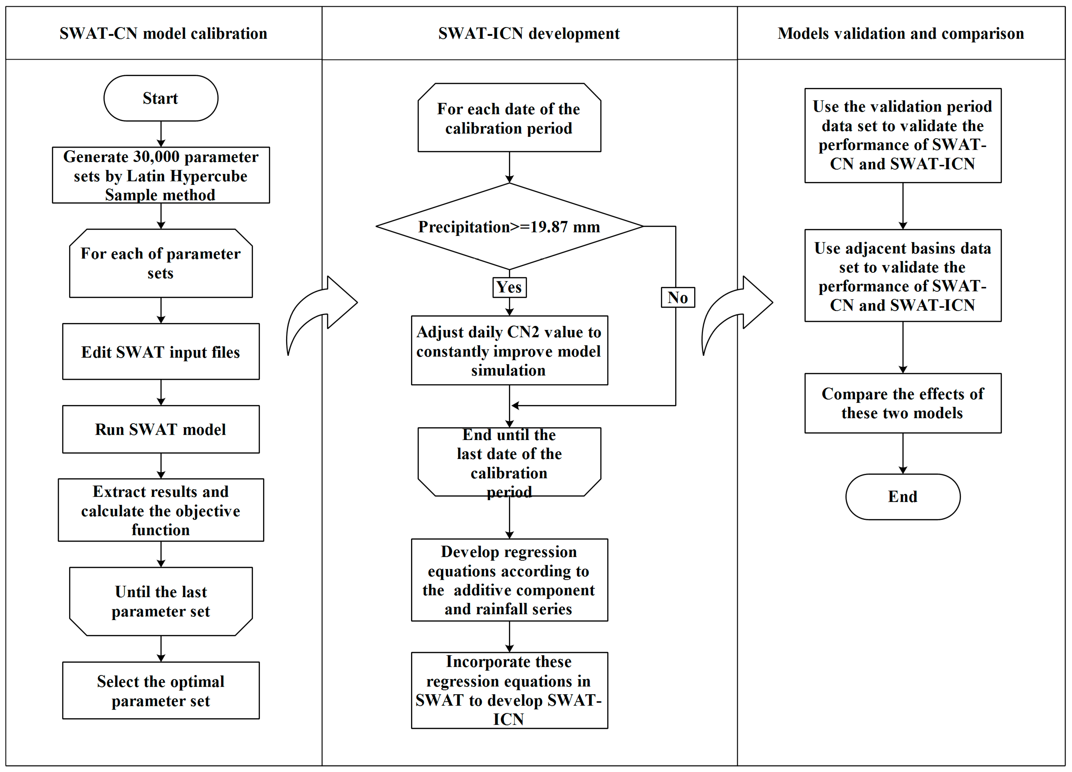
As aforementioned, the validation of the models was performed in two stages. In the first stage, we used the data on the daily observed runoff for January 2007 to December 2010 from the Anxi Watershed to compare the performance of SWAT-CN and SWAT-ICN. In the next stage, we used the data sets of two adjacent watersheds (namely Shanmei and Shilong Watershed) to compare further the performance of these two models. For easy comparison, the performance measures achieved by these two models in the two adjacent basins were also split into two periods consistent with the split scheme adopted for the Anxi daily runoff model. One more thing that needs to be noted is that the “observed base flows” used to compare the performance of SWAT-CN and SWAT-ICN in predicting streamflow components were derived by separating observed stream flows into base flows and direct flows using an automated digital filter technique [36,37]. Although the filter technique has no true physical basis, it has been extensively tested against other automated techniques (e.g., the PART model) and manual separation methods. It has proven to be objective and reproducible in other studies [38,39,40,41]. The processes used in calibrating the SWAT-CN model, developing the SWAT-ICN model, and validating both models are illustrated in Figure 2.
3. Results
3.1. Development of the RE
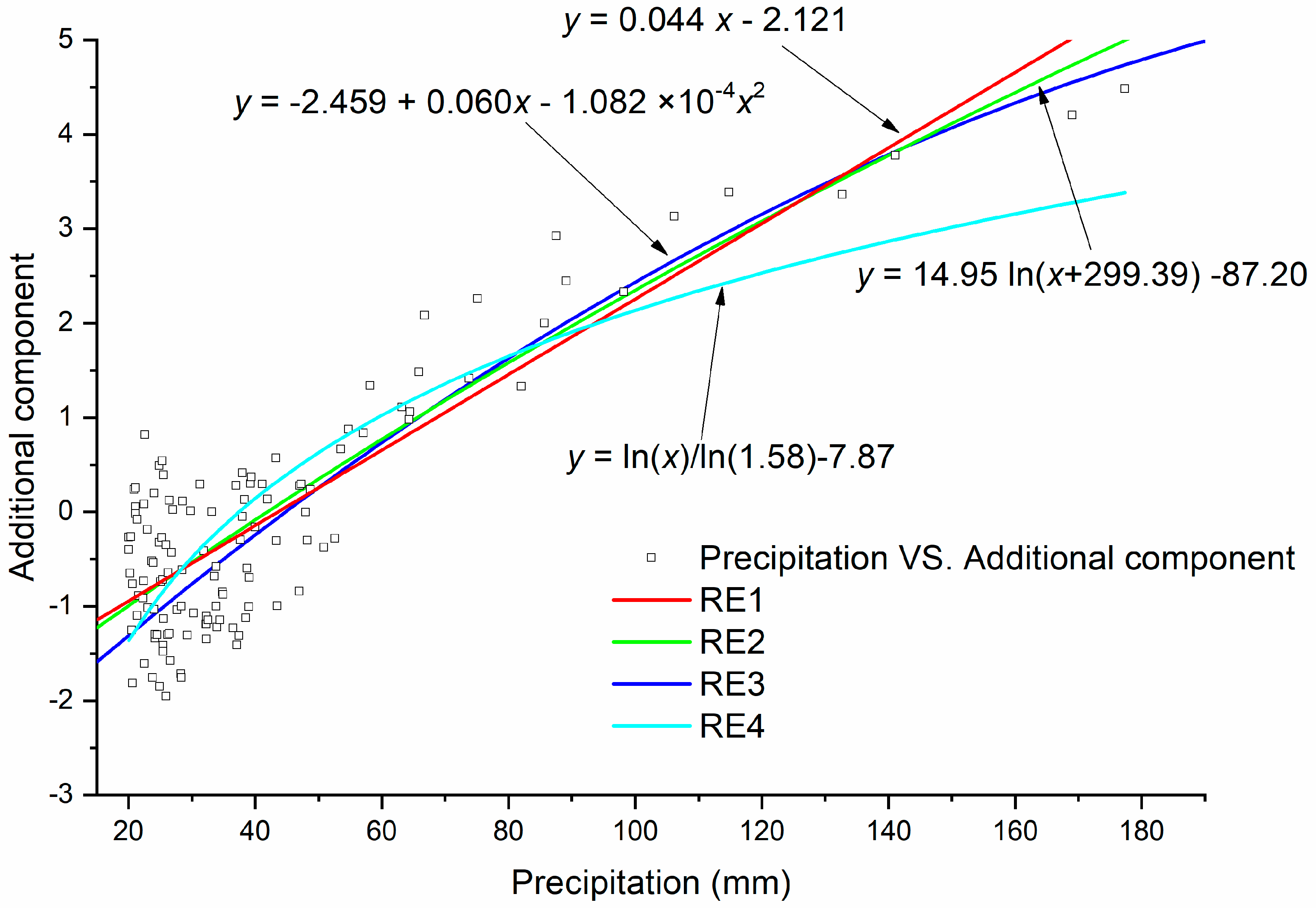
In this study, two rounds of calibration were conducted to set up the daily runoff model for Anxi Watershed (one for the SWAT-CN and one for the SWAT-ICN runoff model, respectively). The first round calibration (left part of Figure 2) was used to identify the optimal parameter set for the SWAT-CN runoff model (Table 1). After the second round of calibration (fine-tune calibration) was finished, 123 AC-rainfall pairs were used to develop the regression equations, which explain the relation of AC to rainfall intensity (daily rainfall depth). Four potential regression equations (Table 2; Figure 3) were derived and evaluated. Overall, all four of the regression equations achieved similar performance. Nevertheless, we found that regression Equation (3) (RE3) was the best among these equations in terms of describing the trend of AC to rainfall depth (Figure 3), and for overall fit of simulated to observed streamflow (with an ENS and R2 of 0.89 and 0.88, respectively). RE2 was the best option for simulation of overall streamflow volumes (with the smallest PBIAS), but was less effective than RE3 in capturing the trend of AC to rainfall depth (the ENS and R2 are slight small or equal to those of RE3). RE1 and RE4 were generally less effective than RE2 and RE3. Based on overall consideration of their abilities in capturing the trend of AC to rainfall depth, and in providing accurate simulation of daily streamflow, RE2 was chosen to incorporate into SWAT-ICN.
It is noteworthy that we only chose 123 daily rainfall events of which the rainfall depth exceeded or equaled 19.87 mm for use in the second-round calibration. The reason was that, for events with rainfall depth less than 19.87 mm, there is little opportunity to generate overland flow due to the rain water lost through initial abstraction. With less rainfall, the amount of runoff generated is greatly affected by the previous soil water content, thus the effects of rainfall intensity on runoff generation should receive less emphasis, or could be omitted in this case. We also noted that these regression equations generate negative values close to minimum precipitation threshold (19.87 mm) adopted in this study. We believed that the occurrences of negative values for the AC are due to overestimating CN in the parameterization procedure. Thus the regression equations generate negative values, at where the precipitation is close to the threshold value, to compensate the overestimated CN. We would suggest followers to initiate the CN values with relative small values and allow the AC to be adjusted within a wider range.
3.2. Daily Streamflow Simulations
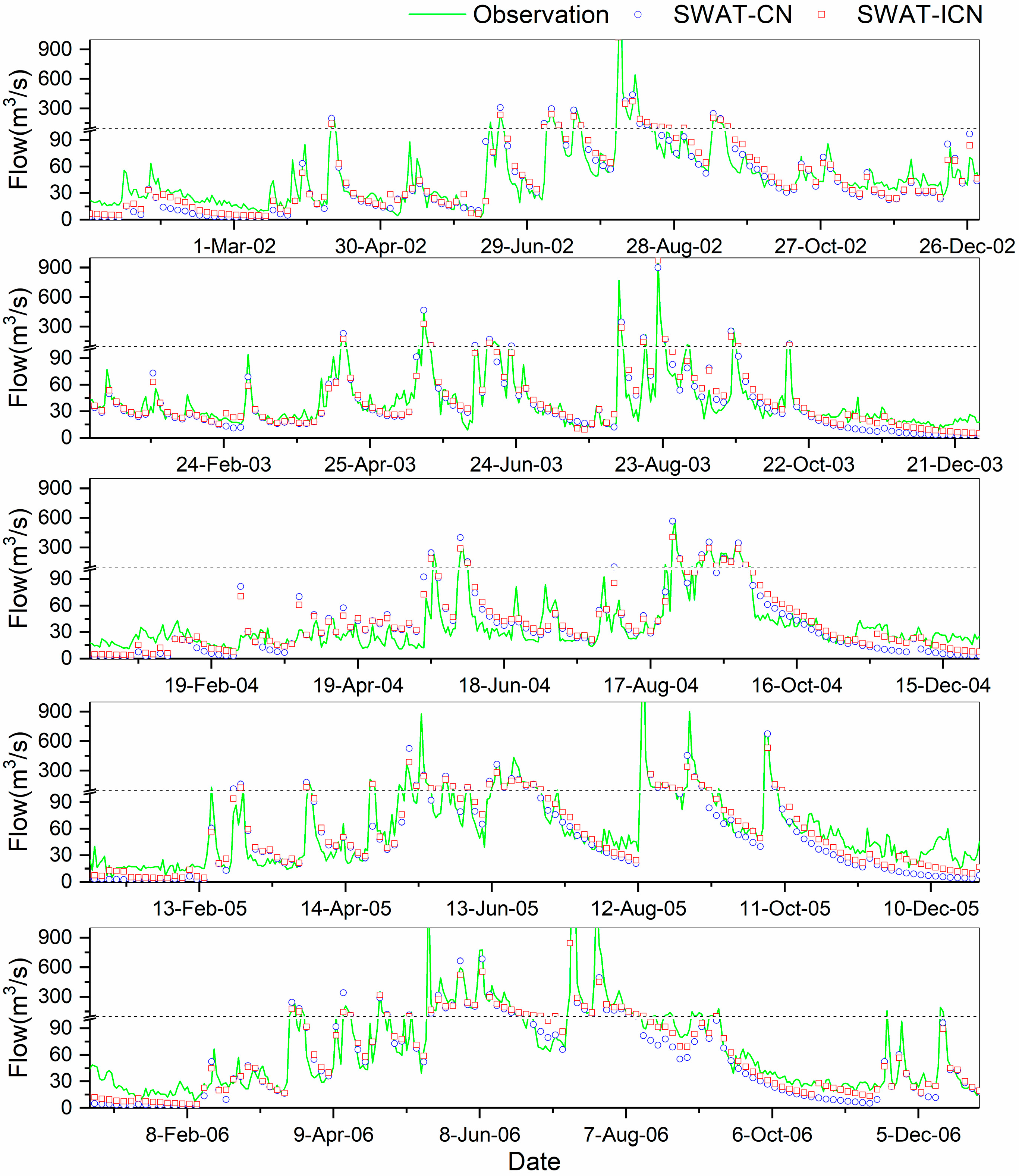
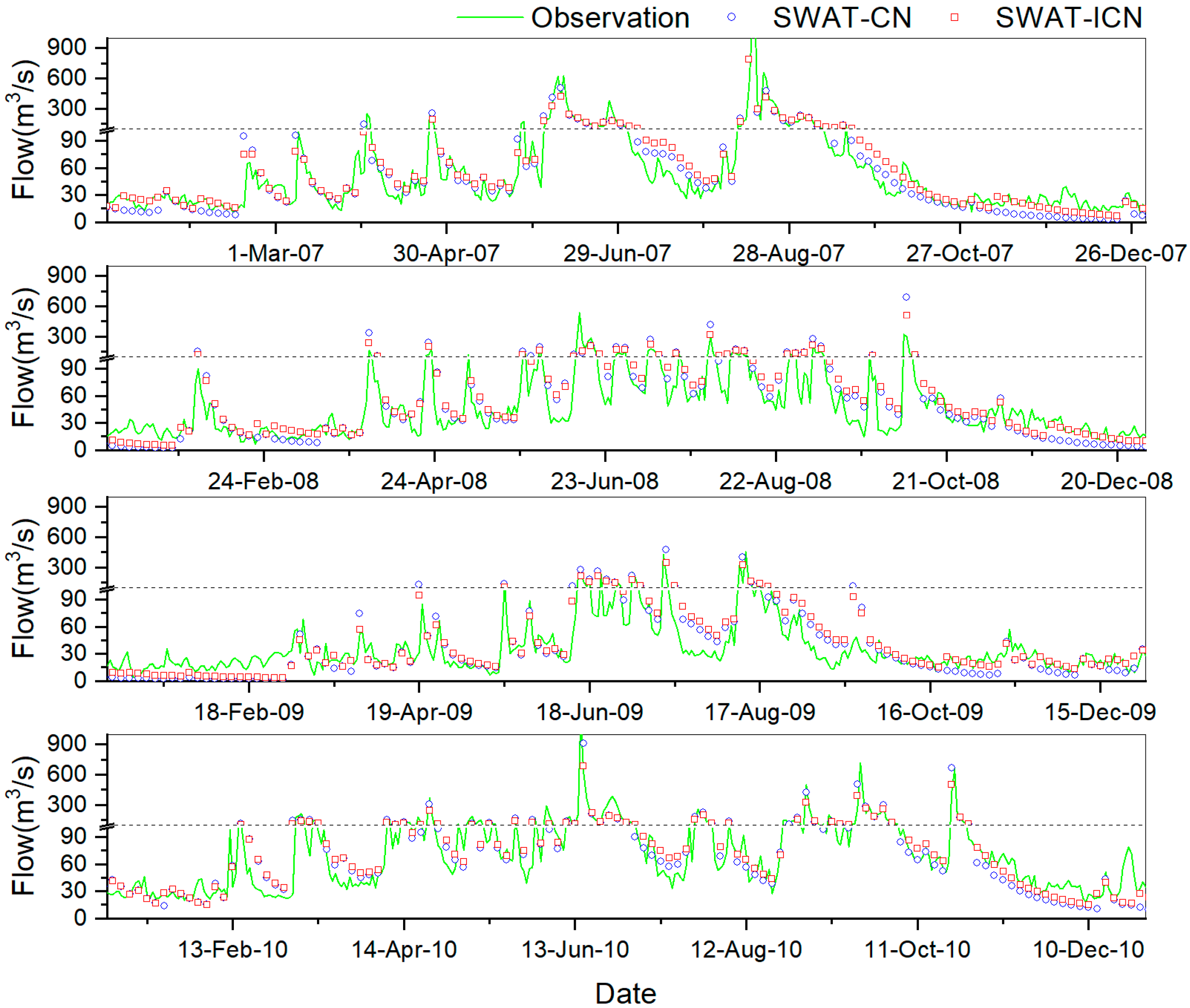
Figure 4 shows the hydrographs of the optimal solutions of SWAT-CN and SWAT-ICN runoff models for the calibration period at Anxi Watershed. The simulated results for both models are generally in agreement with observations indicating the potential of these two models to reasonably simulate streamflow. Nevertheless, there were some high-flow events that both models failed to simulate accurately. Similar results could also be observed from hydrographs during the validation period for Anxi Watershed (Figure 5). These results indicate that the parameter sets deriving from the calibration processes could reasonably represent the characteristics of the Anxi Watershed.
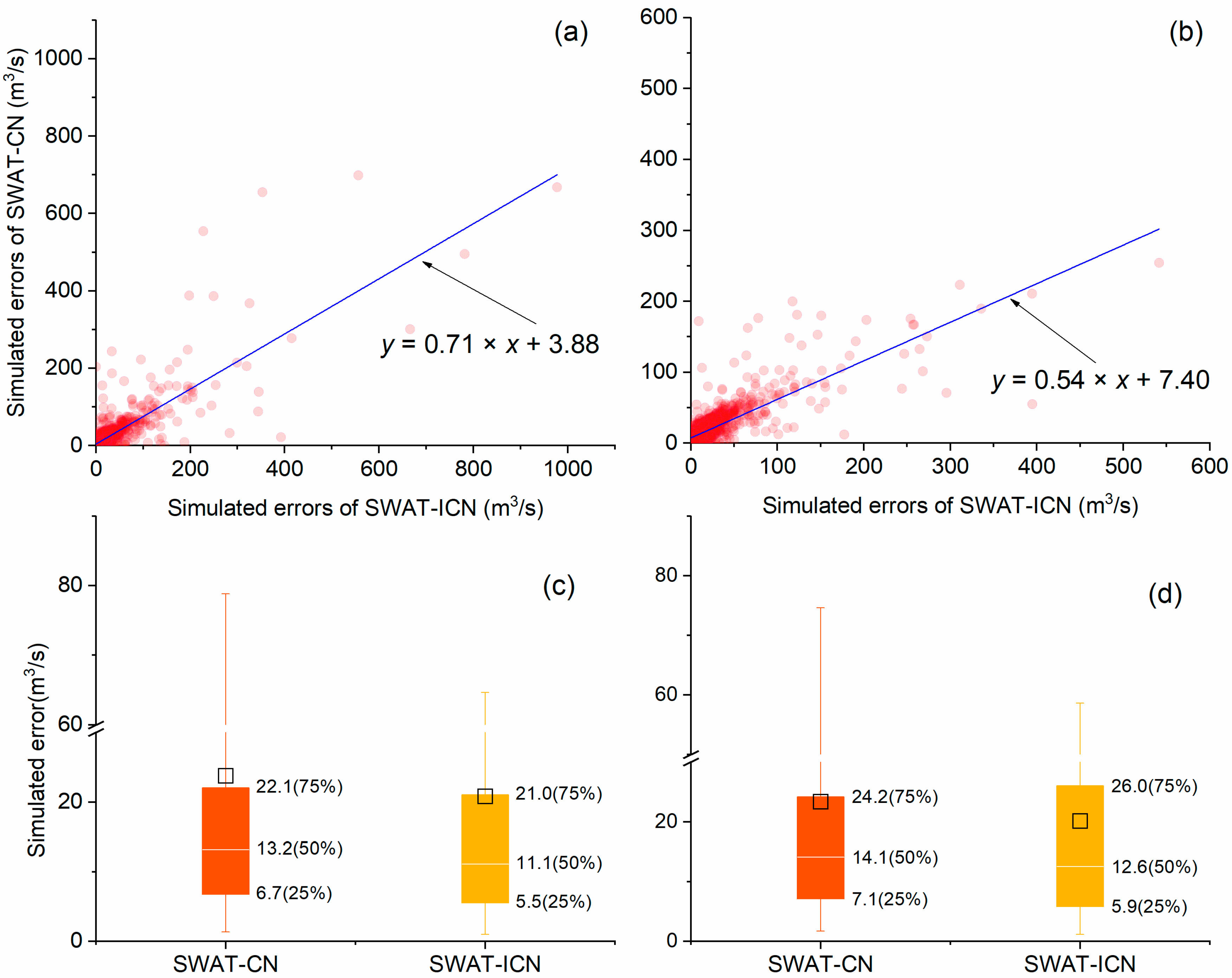
For easy comparisons of the performance of SWAT-CN and SWAT-ICN, the simulation errors SWAT-CN vs. SWAT-ICN are plotted in Figure 6a,b, respectively, for calibration and validation periods. It is clear from these scatterplots that the SWAT-ICN model simulated errors are generally smaller than those of the SWAT-CN model. According to the fit line equations, it can be said that SWAT-ICN was more successful at reproducing the daily streamflows during both calibration and validation periods. This can also be judged from Figure 6c,d, which present the statistics of the simulated errors of SWAT-CN and SWAT-ICN, respectively. The mean, median, and 5th, 25th, 75th and 95th percentiles of errors from the SWAT-ICN were smaller than those of the SWAT-CN for both calibration and validation periods, with the exception of the 75th percentile for validation period, in which the 75th percentile of SWAT-ICN was slightly higher than that of SWAT-CN model.
In addition to visual inspection of the daily streamflow simulations, statistic measures including ENS, R2 and PBIAS were also used to evaluate the performance of the two models. Table 3 shows the values of the ENS, R2, and PBIAS of SWAT-CN and SWAT-ICN runoff models for the Anxi, Shanmei, and Shilong watersheds. For easy comparison, the optimal measures achieved by these two models are presented in bold type. In the calibration period, the PBIAS of SWAT-ICN for the Anxi Watershed is slightly worse than that of SWAT-CN with a small increase (0.1%). In contrast to PBIAS, both ENS and R2 of SWAT-ICN for Anxi Watershed are better than those of SWAT-CN, with increase of 0.05% and 0.04%, respectively. Performance measures of SWAT-ICN for the Anxi Watershed in the validation period also suggests an improvement of SWAT-ICN, because the ENS, R2, and PBIAS for SWAT-ICN were (0.86%, 0.85%, and 9.75%), respectively, compared to (0.79%, 0.78%, and 10.52%), respectively, for SWAT-CN. Improvements of SWAT-ICN could also be observed from the performance measures for the adjacent Shanmei and Shilong Watersheds. In summary, the overall qualities of SWAT-ICN for both the calibration and validation periods in all three watersheds were better than or close to those of SWAT-CN. It is noted that we tried a relatively larger number (30,000) of model iterations in the calibration of SWAT-CN. Thus, we believe that the improvement of SWAT-ICN was not due to insufficient calibration of SWAT-CN, but mostly due to the ability of this model to account reasonably for the effects of rainfall intensity on runoff generation.
In this study watershed, the flashy convective storms and sea-based typhoons contribute approximately 38% of the annual precipitation in the wet period (May–October). During these events, the runoff tends to be generated by infiltration excess due to the high-intensity rainfall. In contrast, the runoff is generated mainly by saturation excess processes in areas of bare soil, riparian zones, and impermeable surfaces of urban land during the dry period. Therefore, it is important for models to account for the seasonal variability of the runoff generation mechanics for proper rainfall-runoff modelling in Jinjiang and similar watersheds. To evaluate the ability of SWAT-ICN and SWAT-CN to account for the seasonal variability of runoff generation, the observed and simulated series were split into dry and wet series, and the performance measures were calculated for these two series (Table 4).
When the wet and dry series were separately considered, improvements of ENS for SWAT-ICN over SWAT-CN were observed from the dry and wet series for all three watersheds, in both the calibration and validation period (Table 4). Except for the R2 of the dry series for the Shanmei and Shilong Watersheds in the calibration period (0.64 and 0.63 for SWAT-CN and SWAT-ICN, respectively, for Shanmei Watershed; and both 0.66 for Shilong Watershed), the R2 values for SWAT-ICN were higher than those for SWAT-CN, implying a better fit of simulation to observation for SWAT-ICN. Improvements of PBIAS could also be observed for both dry and wet series during calibration and validation for the Anxi Watershed. However, the PBIAS values decreased slightly during calibration for the Shanmei and Shilong watersheds in both the dry and wet series. Overall, SWAT-ICN could reasonably account for the seasonal variability of the runoff generation mechanics in Jinjiang, thereby providing better performance than with SWAT-CN. There are two possible reasons for the improved performance of SWAT-ICN. First, by considering the effects of rainfall intensity, SWAT-ICN offered more accurate runoff estimation, especially for large rainfall events (of which the daily depth exceeds the threshold value), this undoubtedly led to better performance of SWAT-ICN in wet periods (during which the vast majority of large rainfall events occur). Second, SWAT-ICN could accurately mimic the flow pathways and thus provide more accurate estimation of the infiltration and ground water storage, which in turn contributed to more accurate base-flow simulation, the main component of the streamflow in dry periods.
3.3. Annual Extreme Flow Simulations
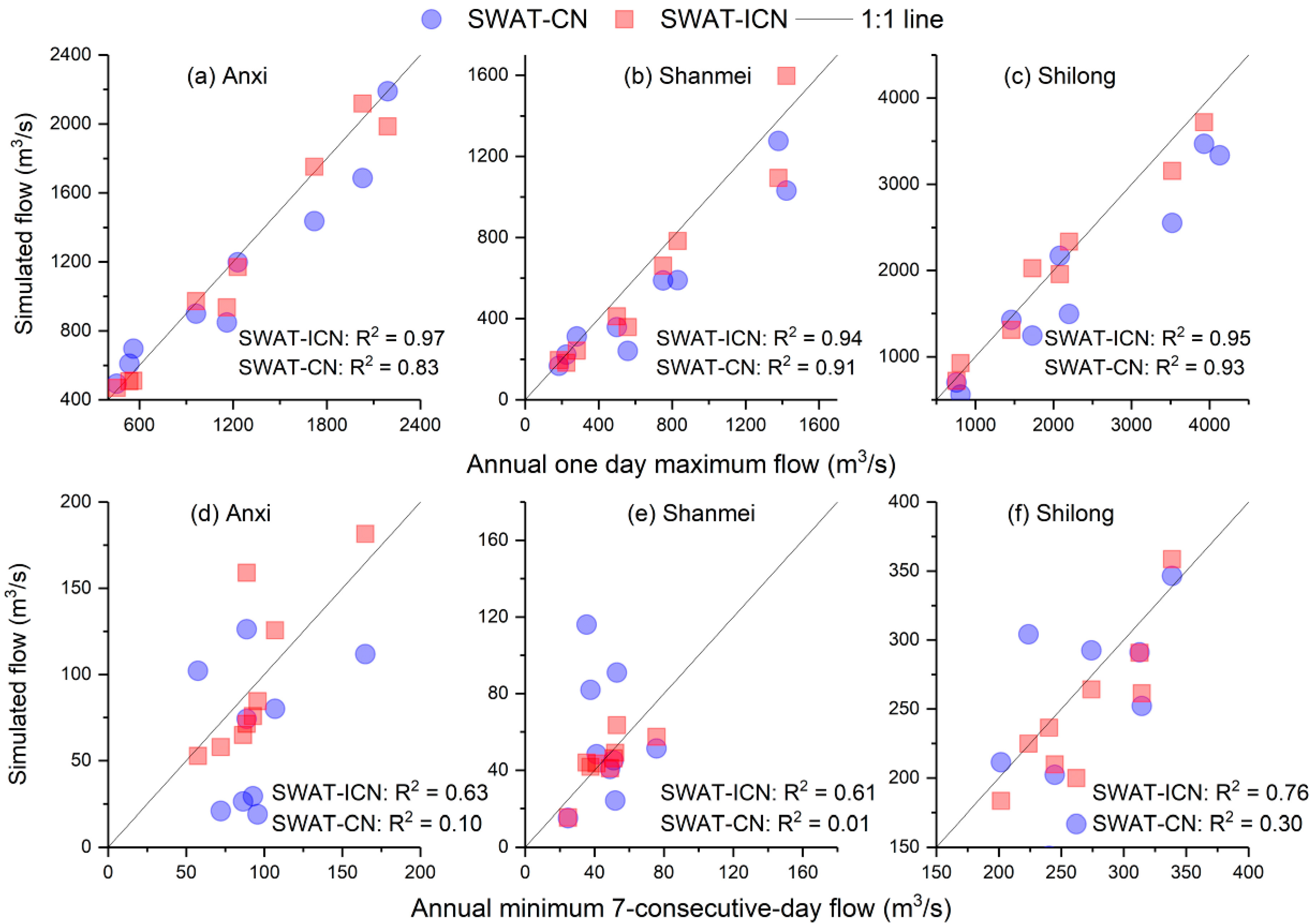
Rainfall intensity may exert great influence over the processes that generate low and high flows. Therefore accurate reproduction of these extreme events is a crucial index to the merit of a model. With this purpose, the annual one day maximum flow (1-DMF) and the minimum flow of seven consecutive days (7-CDMF), as well as their corresponding simulated results for SWAT-ICN and SWAT-CN, were calculated for 2002–2010. In Figure 7, the 1-DMFs vs. their corresponding simulated flows of SWAT-ICN and SWAT-CN are plotted as a, b, and c; for Anxi, Shanmei, and Shilong Watershed, respectively. Overall, the simulated flows of SWAT-ICN fit the 1-MDFs better than SWAT-CN did in all nine years. The R2 values, which demonstrate the goodness of fit of the simulated flows of SWAT-CN to the 1-DMFs, were consistently lower than those for SWAT-ICN in all three watersheds of the Jinjiang Watershed. The R2 values were 0.83, 0.91, and 0.93 for SWAT-CN and 0.97, 0.94, and 0.95 for SWAT-ICN; for Anxi, Shanmei, and Shilong Watershed, respectively.
To examine the performance of these two models in simulating extreme low flows, the 7-CDMFs vs. their corresponding simulated flows of SWAT-ICN and SWAT-CN are plotted in plot d, e, and f of Figure 7; for Anxi, Shanmei, and Shilong Watershed, respectively. The R2 values, which describe the goodness of fit of the simulated flows of SWAT-ICN to the 7-CDMFs were significantly larger than those of SWAT-CN, indicating a great improvement of SWAT-ICN over SWAT-CN in reproducing the extreme low-flow events. The improvements in respect to the extreme low flow simulations may result from the more accurate CN estimations that were facilitated by the proposed method. The amount of water that will finally became surface water and infiltrate into soil is determined by the CN value, therefore more accurate CN values will undoubtedly lead to a more accurate prediction of the surface flow and have more chances to derive accurate ground water estimation as accurate estimation of infiltration water is an essential precondition for precisely ground water estimation. In other word, the accurate estimation of infiltration water does not guarantee accurate ground water estimation, however it would be impossible to derive accurate ground water estimation without accurate infiltration water estimation. It is interesting to note that for those extreme low-flow events, there are seldom rainfall events with rainfall depth exceeding or equal to 19.87 mm; hence, there are no CN adjustments. We deduce that the improvements of the SWAT-ICN in simulating extreme low flows are not a direct result of the adjustment of the CN values of intensive rainfall events, but an indirect result of the CN adjustments. As we have discussed above, the proposed method may contribute to an accurate estimation of ground water storage, which is usually recharged by the infiltrated water during wet periods and discharge to stream as base flow during dry periods. In general, the SWAT-ICN provides a more accurate estimation of the infiltration water, and thus may lead to better the ground water storage and base flow simulations as well as extreme low flows. Because base flow is the primary component of streamflow in extreme low-flow events, the accurate prediction of base flow can exert great influence on the performance of low-flow simulations.
3.4. Base Flow Simulations
SWAT-ICN is assumed to better account for the effect of rainfall intensity on runoff generation; therefore, it is assumed to provide more accurate prediction of the lumped total stream flow as well as its components (i.e., the direct and base flows). To verify this hypothesis, statistical measures that describe the accuracy of SWAT-ICN and SWAT-CN in simulating base flows were calculated in Table 5. Significant improvement was achieved by using SWAT-ICN, compared with SWAT-CN. For example, the ENSs, R2 values, and PBIASs of SWAT-ICN for the Anxi Watershed are 0.55 and 0.53, 0.63 and 0.60, and −14.26% and −15.66%, respectively, for calibration and validation. For SWAT-CN, the equivalent values were 0.34 and 0.37, 0.50 and 0.58, and −20.80% and −21.28%, respectively. Improvements with SWAT-ICN can also be observed from the performance measures of the adjacent Shanmei and Shilong Watersheds. The measures for SWAT-CN were consistently poorer than those for SWAT-ICN for both calibration and validation. These results directly indicate that SWAT-ICN can more accurately mimic the flow pathways than SWAT-CN. This is because the CN adjustments in wet period can provide a more accurate infiltration water estimation, which in turn can lead to a more accurate estimation of ground water storage, which discharge to stream as base flow during dry periods. Because base flows are contributed mostly by ground water storage, the improvement of SWAT-ICN in better estimating soil infiltration hence indirectly results in more accurate base flow simulation.
3.5. Advantages, Disadvantages, and Future Work
The test results suggest that the SWAT-ICN model can more accurately simulate processes in terms of stream flow, base flow, and annual extreme flow; and can better capture the seasonal variability of runoff generation as well. This is due to the ability of the SWAT-ICN model to account for the effects of rainfall intensity on runoff generation. The direct flows and base flows are the vehicles by which pollutants are transported; thus, the SWAT-ICN provides more accurate representation of the water flow amounts, pathways, and source areas. This has great significance for water resource management, flood prediction, soil erosion, and non-point source pollution modelling. Besides these benefits, SWAT-ICN (incorporating the improved curve method) also shares the advantages of the SCS-CN method. The most important one is that this method does not require sub-daily precipitation data (which makes it impossible to use in data-scarce areas).
The SWAT-ICN model provides a simple and robust means of estimating excess rainfall; however, there are some limitations of this model. For example, when the regression equations that explain the relation of AC to rainfall intensity is incorporated into SWAT to develop SWAT-ICN, additional parameters need to be determined or calibrated. This inevitably places an extra burden on the calibration of SWAT-ICN and may exacerbate the over-parameterized problems with SWAT. The SWAT-ICN model provides a logical direction for research aiming to improve the existing SCS-CN method to better account for the effects of rainfall intensity on rainfall-runoff generation. However, in the future, it is necessary to test and verify this model in watersheds with distinctly different rainfall patterns. Another possible research direction would involve using isotope tracing methods to further examine the ability of SWAT-ICN in predicting base flows.
4. Summary and Conclusions
A given amount of rainfall may generate totally different runoff volumes and flow pathways due to the effects of rainfall intensity. In this study, we proposed a method to better estimate CN value by adding a regression model that can better account for the effects of rainfall intensity on rainfall-runoff generation processes. This method was developed by adding an addition component (AC) to the existing CN equation. This was determined by a regression equation developed from the relationship between the AC and observed rainfall series after fine-tuned calibration processes. With the purpose of evaluating the newly developed method, we incorporated this regression equation into SWAT and compared the performance of this new version of SWAT (SWAT-ICN) and the original SWAT (SWAT-CN) with data from the Anxi Watershed for the periods January 2007 to December 2010, and with data sets for two adjacent watersheds (the east branch and downstream of the Jinjian Watershed) for the periods January 2001 to December 2010.
The assessment results suggest that both the SWAT-ICN and SWAT-CN models had a comparable and satisfactory performance in predicting total stream flow in the study watersheds. Nevertheless, the SWAT-ICN model more accurately reproduced simulated processes in terms of stream flow, base flow, and annual extreme flow; and better captured the seasonal variability of runoff generation as well. This is because that SWAT-ICN more reasonably accounts for the effects of rainfall intensity on runoff generation and thus more accurately mimics the flow pathways. The assessments with the data sets of the two adjacent watersheds demonstrate the potential for the SWAT-ICN model to be used in other watersheds with distinct rainfall patterns.
While the SWAT-ICN model provides a logical research direction aiming to improve the existing SCS-CN method to better account for the effects of rainfall intensity on rainfall-runoff generation, it still needs to be further tested and verified in watersheds with distinctly different rainfall pattern, across various physiographic conditions.
Author Contributions
Conceptualization, X.C. and D.Z.; methodology, D.Z.; software, D.Z. validation, Q.L., D.Z. and T.C.; writing—original draft preparation, D.Z. and Q.L.; writing—review and editing, X.C.; supervision, X.C.
Funding
This research was funded by the Natural Science Foundation of China, grant number 41877167, the Natural Science Foundation of Fujian Province, grant number 2018J01481; the Science and Technology Project of Xiamen, grant number 3502Z20183056; the Open Research Fund Program from Fujian Engineering and Research Center of Rural Sewage Treatment and Water Safety, grant number RST201801; and the Talent Project of Xiamen University of Technology, grant number YKJ16017R.
Acknowledgments
The authors appreciate reviewers for their insightful comments and constructive suggestions on our research work. The authors also want to thank editors for their patient and meticulous work for our manuscript.
Conflicts of Interest
The authors declare no conflict of interest.
References
- King, K.W.; Arnold, J.; Bingner, R. Comparison of Green-Ampt and curve number methods on Goodwin Creek watershed using SWAT. Trans. ASABE 1999, 42, 919. [Google Scholar] [CrossRef]
- Grimaldi, S.; Petroselli, A.; Romano, N. Green-Ampt Curve-Number mixed procedure as an empirical tool for rainfall–runoff modelling in small and ungauged basins. Hydrol. Process. 2013, 27, 1253–1264. [Google Scholar] [CrossRef]
- Bulygina, N.; Mcintyre, N.; Wheater, H. A comparison of rainfall-runoff modelling approaches for estimating impacts of rural land management on flood flows. Hydrol. Res. 2013, 44, 467–483. [Google Scholar] [CrossRef]
- Kisi, O.; Shiri, J.; Tombul, M. Modeling rainfall-runoff process using soft computing techniques. Comput. Geosci. 2013, 51, 108–117. [Google Scholar] [CrossRef]
- Shoaib, M.; Shamseldin, A.Y.; Melville, B.W. Comparative study of different wavelet based neural network models for rainfall–runoff modeling. J. Hydrol. 2014, 515, 47–58. [Google Scholar] [CrossRef]
- Futter, M.N.; Erlandsson, M.A.; Butterfield, D.; Whitehead, P.G.; Oni, S.K.; Wade, A.J. PERSiST: A flexible rainfall-runoff modelling toolkit for use with the INCA family of models. Hydrol. Earth Syst. Sci. 2014, 18, 855–873. [Google Scholar] [CrossRef]
- Ficklin, D.; Zhang, M. A comparison of the curve number and green-ampt models in an agricultural watershed. Trans. ASABE 2013, 56, 61–69. [Google Scholar] [CrossRef]
- Wang, X.; Shang, S.; Yang, W.; Melesse, A. Simulation of an agricultural watershed using an improved curve number method in SWAT. Trans. ASABE 2008, 51, 1323–1339. [Google Scholar] [CrossRef]
- Coles, A.E.; McConkey, B.G.; McDonnell, J.J. Climate change impacts on hillslope runoff on the northern Great Plains, 1962–2013. J. Hydrol. 2017, 550, 538–548. [Google Scholar] [CrossRef]
- Alizadeh, M.J.; Kavianpour, M.R.; Kisi, O.; Nourani, V. A new approach for simulating and forecasting the rainfall-runoff process within the next two months. J. Hydrol. 2017, 548, 588–597. [Google Scholar] [CrossRef]
- Garen, D.C.; Moore, D.S. Curve number hydrology in water quality modeling: Uses, abuses, and future directions. J. Am. Water Resour. Assoc. 2005, 41, 377–388. [Google Scholar] [CrossRef]
- Cheng, Q.-B.; Reinhardt-Imjela, C.; Chen, X.; Schulte, A.; Ji, X.; Li, F.-L. Improvement and comparison of the rainfall–runoff methods in SWAT at the monsoonal watershed of Baocun, Eastern China. Hydrol. Sci. J. 2016, 61, 1460–1476. [Google Scholar] [CrossRef]
- Michel, C.; Andréassian, V.; Perrin, C. Soil Conservation Service Curve Number method: How to mend a wrong soil moisture accounting procedure? Water Resour. Res. 2005, 41, W02011. [Google Scholar] [CrossRef]
- Jeong, J.; Kannan, N.; Arnold, J.; Glick, R.; Gosselink, L.; Srinivasan, R. Development and Integration of Sub-hourly Rainfall–Runoff Modeling Capability Within a Watershed Model. Water Resour. Manag. 2010, 24, 4505–4527. [Google Scholar] [CrossRef]
- White, E.D.; Feyereisen, G.W.; Veith, T.L.; Bosch, D.D. Improving daily water yield estimates in the Little River watershed: SWAT adjustments. Trans. ASABE 2009, 52, 69–79. [Google Scholar] [CrossRef]
- White, E.D.; Easton, Z.M.; Fuka, D.R.; Collick, A.S.; Adgo, E.; McCartney, M.; Awulachew, S.B.; Selassie, Y.G.; Steenhuis, T.S. Development and application of a physically based landscape water balance in the SWAT model. Hydrol. Process. 2011, 25, 915–925. [Google Scholar] [CrossRef]
- Zhang, D.; Chen, X.; Yao, H.; Lin, B. Improved calibration scheme of SWAT by separating wet and dry seasons. Ecol. Model. 2015, 301, 54–61. [Google Scholar] [CrossRef] [Green Version]
- Romkens, M.J.M.; Baumhardt, R.L.; Parlange, M.B.; Whisler, F.D.; Parlange, J.Y.; Prasad, S.N. Rain-induced surface seals: Their effect on ponding and infiltration. Ann. Geophys. 1986, 4, 417–424. [Google Scholar]
- Hawke, R.M.; Price, A.G.; Bryan, R.B. The effect of initial soil water content and rainfall intensity on near-surface soil hydrologic conductivity: A laboratory investigation. Catena 2006, 65, 237–246. [Google Scholar] [CrossRef]
- Wu, X.; Zhang, L. Research on Effecting Factors of Precipitation’s Redistribution of Rainfall Intensity, Gradient and Cover Ratio. J. Soil Water Conserv. 2006, 20, 28–30. [Google Scholar]
- Huang, J.; Wu, P.; Zhao, X. Effects of rainfall intensity, underlying surface and slope gradient on soil infiltration under simulated rainfall experiments. Catena 2013, 104, 93–102. [Google Scholar] [CrossRef]
- Wei, W.; Jia, F.; Yang, L.; Chen, L.; Zhang, H.; Yu, Y. Effects of surficial condition and rainfall intensity on runoff in a loess hilly area, China. J. Hydrol. 2014, 513, 115–126. [Google Scholar] [CrossRef] [Green Version]
- Wang, H.; Gao, J.E.; Zhang, M.-J.; Li, X.-H.; Zhang, S.-L.; Jia, L.-Z. Effects of rainfall intensity on groundwater recharge based on simulated rainfall experiments and a groundwater flow model. Catena 2015, 127, 80–91. [Google Scholar] [CrossRef]
- Beven, K.; Germann, P. Macropores and water flow in soils. Water Resour. Res. 1982, 18, 1311–1325. [Google Scholar] [CrossRef]
- Fohrer, N.; Berkenhagen, J.; Hecker, J.M.; Rudolph, A. Changing soil and surface conditions during rainfall. Catena 1999, 37, 355–375. [Google Scholar] [CrossRef]
- Kim, N.W.; Lee, J. Temporally weighted average curve number method for daily runoff simulation. Hydrol. Process. 2008, 22, 4936–4948. [Google Scholar] [CrossRef]
- Khan, A.; Koch, M. Correction and informed regionalization of precipitation data in a high mountainous region (Upper Indus Basin) and its effect on SWAT-modelled discharge. Water 2018, 10, 1557. [Google Scholar] [CrossRef]
- Kumarasamy, K.; Belmont, P. Calibration Parameter Selection and Watershed Hydrology Model Evaluation in Time and Frequency Domains. Water 2018, 10, 1. [Google Scholar] [CrossRef]
- Zhang, D.; Chen, X.; Yao, H.; James, A. Moving SWAT model calibration and uncertainty analysis to an enterprise Hadoop-based cloud. Environ. Model. Softw. 2016, 84, 140–148. [Google Scholar] [CrossRef]
- Lin, B.; Chen, X.; Yao, H.; Chen, Y.; Liu, M.; Gao, L.; James, A. Analyses of landuse change impacts on catchment runoff using different time indicators based on SWAT model. Ecol. Indic. 2015, 58, 55–63. [Google Scholar] [CrossRef]
- Zhang, D.; Chen, X.; Yao, H. Development of a prototype web-based decision support system for watershed management. Water 2015, 7, 780–793. [Google Scholar] [CrossRef]
- Nash, J.; Sutcliffe, J.V. River flow forecasting through conceptual models part I—A discussion of principles. J. Hydrol. 1970, 10, 282–290. [Google Scholar] [CrossRef]
- Gupta, H.V.; Sorooshian, S.; Yapo, P.O. Status of automatic calibration for hydrologic models: Comparison with multilevel expert calibration. J. Hydrol. Eng. 1999, 4, 135–143. [Google Scholar] [CrossRef]
- Lin, M.; Chen, X.; Chen, Y.; Yao, H. Improving calibration of two key parameters in Hydrologic Engineering Center hydrologic modelling system, and analysing the influence of initial loss on flood peak flows. Water Sci. Technol. 2013, 68, 2718–2724. [Google Scholar] [CrossRef] [PubMed]
- McKay, M.D.; Beckman, R.J.; Conover, W.J. A comparison of three methods for selecting values of input variables in the analysis of output from a computer code. Technometrics 2000, 42, 55–61. [Google Scholar] [CrossRef]
- Arnold, J.G.; Allen, P.M. Automated methods for estimating baseflow and ground water recharge from streamflow records. J. Am. Water Resour. Assoc. 1999, 35, 411–424. [Google Scholar] [CrossRef]
- Gebert, W.A.; Radloff, M.J.; Considine, E.J.; Kennedy, J.L. Use of Streamflow Data to Estimate Base Flow/Ground-Water Recharge for Wisconsin. J. Am. Water Resour. Assoc. 2007, 43, 220–236. [Google Scholar] [CrossRef]
- Rutledge, A.; Daniel, C. Testing an Automated Method to Estimate Ground-Water Recharge from Streamflow Records. Ground Water 1994, 32, 180–189. [Google Scholar] [CrossRef]
- Luo, Y.; Arnold, J.; Allen, P.; Chen, X. Baseflow simulation using SWAT model in an inland river basin in Tianshan Mountains, Northwest China. Hydrol. Earth Syst. Sci. 2012, 16, 1259–1267. [Google Scholar] [CrossRef] [Green Version]
- Szilagyi, J. Sensitivity analysis of aquifer parameter estimations based on the Laplace equation with linearized boundary conditions. Water Resour. Res. 2003, 39, 280–304. [Google Scholar] [CrossRef]
- Szilagyi, J. Heuristic continuous base flow separation. J. Hydrol. Eng. 2004, 9, 311–318. [Google Scholar] [CrossRef]
Figure 1.
Topography and grain system of Jinjiang watershed (a) and its three sub-watersheds: the Shanmei (b), Anxi (c), and Shilong (d) Watersheds.
Figure 1.
Topography and grain system of Jinjiang watershed (a) and its three sub-watersheds: the Shanmei (b), Anxi (c), and Shilong (d) Watersheds.

Figure 2.
Flow diagram of the calibration, development and validation process of SWAT-CN and SWAT-ICN.
Figure 2.
Flow diagram of the calibration, development and validation process of SWAT-CN and SWAT-ICN.

Figure 3.
Regression models that describe the relation of additional component to rainfall intensify (daily rainfall depth).
Figure 3.
Regression models that describe the relation of additional component to rainfall intensify (daily rainfall depth).

Figure 4.
Simulated and observed hydrographs for the calibration period.

Figure 5.
Simulated and observed hydrographs for the validation period.

Figure 6.
Simulated errors of SWAT-ICN versus SWAT-CN for calibration (a) and validation (b) periods, and statistics on the simulated error for calibration (c) and validation (d) periods.
Figure 6.
Simulated errors of SWAT-ICN versus SWAT-CN for calibration (a) and validation (b) periods, and statistics on the simulated error for calibration (c) and validation (d) periods.

Figure 7.
Annual one day maximum flow (1-DMF) of SWAT-ICN versus SWAT-CN for Anxi (a), Shanmei (b), and Shilong (c) gauge stations, and seven consecutive days’ minimum flow (7-CDMF) of SWAT-ICN versus SWAT-CN for Anxi (d), Shanmei (e), and Shilong (f) gauge stations.
Figure 7.
Annual one day maximum flow (1-DMF) of SWAT-ICN versus SWAT-CN for Anxi (a), Shanmei (b), and Shilong (c) gauge stations, and seven consecutive days’ minimum flow (7-CDMF) of SWAT-ICN versus SWAT-CN for Anxi (d), Shanmei (e), and Shilong (f) gauge stations.


Table 1.
Calibrated parameters of Soil and Water Assessment Tool (SWAT) model and their optimal values.
Table 1.
Calibrated parameters of Soil and Water Assessment Tool (SWAT) model and their optimal values.
| ID | Parameter | Meaning | Range | Optimal Value |
|---|---|---|---|---|
| 1 | CANMX | Maximum canopy storage (mm) | 0–100 | 19.222 |
| 2 | ESCO | Soil evaporation compensation factor | 0–1.0 | 0.175 |
| 3 | EPCO | Plant uptake compensation factor | 0–1.0 | 0.499 |
| 4 | ALPHA_BNK | Base flow alpha factor for bank storage | 0–1.0 | 0.749 |
| 5 | ALPHA_BF | Base flow alpha factor (days) | 0–1.0 | 0.965 |
| 6 | SOL_AWC | Available water capacity of the soil layer | 0–1.0 | 0.447 |
| 7 | GWQMN | Threshold depth of water in shallow aquifer required before groundwater flow will occur (mm H2O) | 0–500 | 0.236 |
| 8 | RCHRG_DP | Deep aquifer percolation fraction | 0–1.0 | 0.294 |
Table 2.
Regression equations that describe the relation between additive component and rainfall intensify (daily rainfall depth) and their performances.
Table 2.
Regression equations that describe the relation between additive component and rainfall intensify (daily rainfall depth) and their performances.
| ID | Regression Equation | R2* | Parameters | Performance Measures (2002 to 2006) | ||
|---|---|---|---|---|---|---|
| ENS | R2 | PBIAS (%) | ||||
| RE1 | y = a + bx | 0.73 | a = −1.744 b = 0.040 | 0.87 | 0.86 | 1.51 |
| RE2 | y = a − bln(x + c) | 0.74 | a = −87.20 b = −14.95 c = 299.39 | 0.88 | 0.88 | 0.80 |
| RE3 | y = a + bx + cx2 | 0.78 | a = −2.459 b = 0.060 c = −1.082 × 10⁻⁴ | 0.89 | 0.88 | 1.23 |
| RE4 | y = ln(x)/ln(a) + b | 0.60 | a = 1.58 b = −7.87 | 0.84 | 0.83 | 1.07 |
R2* is coefficient of determination used to describe the relation of AC to rainfall depth.
Table 3.
Performance measures of SWAT-ICN and SWAT-CN in Anxi, Shanmei, and Shilong watersheds for calibration and validation period.
Table 3.
Performance measures of SWAT-ICN and SWAT-CN in Anxi, Shanmei, and Shilong watersheds for calibration and validation period.
| Gauge | Model | Calibration (2002–2006) | Validation (2007–2010) | ||||
|---|---|---|---|---|---|---|---|
| ENS | R2 | PBIAS (%) | ENS | R2 | PBIAS (%) | ||
| Anxi | SWAT-CN | 0.83 | 0.84 | −0.70 | 0.79 | 0.78 | 10.52 |
| SWAT-ICN | 0.88 | 0.88 | −0.80 | 0.86 | 0.85 | 9.75 | |
| Shanmei | SWAT-CN | 0.84 | 0.87 | −0.27 | 0.82 | 0.85 | 7.26 |
| SWAT-ICN | 0.89 | 0.89 | −1.69 | 0.87 | 0.87 | 4.66 | |
| Shilong | SWAT-CN | 0.86 | 0.87 | 6.86 | 0.77 | 0.82 | 7.67 |
| SWAT-ICN | 0.89 | 0.89 | 5.33 | 0.84 | 0.85 | 5.45 | |
Table 4.
Seasonal performance measures of SWAT-ICN and SWAT-CN in Anxi, Shanmei, and Shilong subbasins for calibration and validation period.
Table 4.
Seasonal performance measures of SWAT-ICN and SWAT-CN in Anxi, Shanmei, and Shilong subbasins for calibration and validation period.
| Series | Gauge | Model | Calibration (2002–2006) | Validation (2007–2010) | ||||
|---|---|---|---|---|---|---|---|---|
| ENS | R2 | PBIAS (%) | ENS | R2 | PBIAS (%) | |||
| Dry series | Anxi | SWAT-CN | 0.41 | 0.64 | −19.79 | 0.39 | 0.63 | 3.01 |
| SWAT-ICN | 0.71 | 0.74 | −13.39 | 0.66 | 0.67 | 1.04 | ||
| Shanmei | SWAT-CN | 0.50 | 0.64 | −18.97 | 0.66 | 0.61 | 5.87 | |
| SWAT-ICN | 0.54 | 0.63 | −19.93 | 0.69 | 0.69 | 4.40 | ||
| Shilong | SWAT-CN | 0.06 | 0.66 | −8.56 | 0.45 | 0.63 | 13.01 | |
| SWAT-ICN | 0.35 | 0.66 | −10.23 | 0.69 | 0.72 | 11.91 | ||
| Wet series | Anxi | SWAT-CN | 0.83 | 0.81 | −6.25 | 0.76 | 0.83 | 14.92 |
| SWAT-ICN | 0.88 | 0.87 | 0.33 | 0.87 | 0.88 | 11.65 | ||
| Shanmei | SWAT-CN | 0.84 | 0.82 | −6.55 | 0.87 | 0.87 | 7.72 | |
| SWAT-ICN | 0.89 | 0.89 | −8.35 | 0.90 | 0.91 | 5.22 | ||
| Shilong | SWAT-CN | 0.85 | 0.82 | −4.67 | 0.82 | 0.85 | 10.65 | |
| SWAT-ICN | 0.90 | 0.86 | −6.30 | 0.86 | 0.87 | 8.01 | ||
Table 5.
Performance measures of SWAT-ICN and SWAT-CN in simulating base flow in Anxi, Shanmei, and Shilong subbasins for calibration and validation period.
Table 5.
Performance measures of SWAT-ICN and SWAT-CN in simulating base flow in Anxi, Shanmei, and Shilong subbasins for calibration and validation period.
| Gauge | Model | Calibration (2002–2006) | Validation (2007–2010) | ||||
|---|---|---|---|---|---|---|---|
| ENS | R2 | PBIAS (%) | ENS | R2 | PBIAS (%) | ||
| Anxi | SWAT-CN | 0.34 | 0.50 | −20.80 | 0.37 | 0.58 | −21.28 |
| SWAT-ICN | 0.55 | 0.63 | −14.26 | 0.53 | 0.60 | −15.66 | |
| Shanmei | SWAT-CN | 0.42 | 0.58 | −24.05 | 0.46 | 0.54 | −22.94 |
| SWAT-ICN | 0.58 | 0.64 | −12.56 | 0.66 | 0.68 | −12.04 | |
| Shilong | SWAT-CN | 0.31 | 0.55 | −29.99 | 0.32 | 0.55 | −25.27 |
| SWAT-ICN | 0.50 | 0.60 | −15.66 | 0.51 | 0.60 | −12.98 | |
© 2019 by the authors. Licensee MDPI, Basel, Switzerland. This article is an open access article distributed under the terms and conditions of the Creative Commons Attribution (CC BY) license (http://creativecommons.org/licenses/by/4.0/).
Share and Cite
MDPI and ACS Style
Zhang, D.; Lin, Q.; Chen, X.; Chai, T. Improved Curve Number Estimation in SWAT by Reflecting the Effect of Rainfall Intensity on Runoff Generation. Water 2019, 11, 163. https://doi.org/10.3390/w11010163
AMA Style
Zhang D, Lin Q, Chen X, Chai T. Improved Curve Number Estimation in SWAT by Reflecting the Effect of Rainfall Intensity on Runoff Generation. Water. 2019; 11(1):163. https://doi.org/10.3390/w11010163
Chicago/Turabian StyleZhang, Dejian, Qiaoyin Lin, Xingwei Chen, and Tian Chai. 2019. "Improved Curve Number Estimation in SWAT by Reflecting the Effect of Rainfall Intensity on Runoff Generation" Water 11, no. 1: 163. https://doi.org/10.3390/w11010163
Note that from the first issue of 2016, this journal uses article numbers instead of page numbers. See further details here.