Article

Comparison of Methods to Estimate Lake-Surface-Water Temperature Using Landsat 7 ETM+ and MODIS Imagery: Case Study of a Large Shallow Subtropical Lake in Southern Brazil

by
Matheus Henrique Tavares
1,*,
Augusto Hugo Farias Cunha
1,
David Motta-Marques
1,
Anderson Luís Ruhoff
1,
J. Rafael Cavalcanti
1,
Carlos Ruberto Fragoso, Jr.
2,
Juan Martín Bravo
1,
Andrés Mauricio Munar
3,
Fernando Mainardi Fan
1 and
Lucia Helena Ribeiro Rodrigues
1
1
Instituto de Pesquisas Hidráulicas, Universidade Federal do Rio Grande do Sul, 91501-970 Porto Alegre, Rio Grande do Sul, Brazil
2
Centro de Tecnologia, Universidade Federal de Alagoas, 57072-900 Maceió, Alagoas, Brazil
3
Escuela de Ciencias Agrícolas, Pecuarias y del Medio Ambiente, Universidad Nacional Abierta y a Distancia, 111411 Bogotá, Colombia
*
Author to whom correspondence should be addressed.
Water 2019, 11(1), 168; https://doi.org/10.3390/w11010168
Submission received: 22 November 2018 / Revised: 9 January 2019 / Accepted: 13 January 2019 / Published: 18 January 2019
(This article belongs to the Section Water Quality and Contamination)

Abstract

:
Water temperature regulates many processes in lakes; therefore, evaluating it is essential to understand its ecological status and functioning, and to comprehend the impact of climate change. Although few studies assessed the accuracy of individual sensors in estimating lake-surface-water temperature (LSWT), comparative analysis considering different sensors is still needed. This study evaluated the performance of two thermal sensors, MODIS and Landsat 7 ETM+, and used Landsat methods to estimate the SWT of a large subtropical lake. MODIS products MOD11 LST and MOD28 SST were used for comparison. For the Landsat images, the radiative transfer equation (RTE), using NASA’s Atmospheric Correction Parameter Calculator (AtmCorr) parameters, was compared with the single-channel algorithm in different approaches. Our results showed that MOD11 obtained the highest accuracy (RMSE of 1.05 ° C), and is the recommended product for LSWT studies. For Landsat-derived SWT, AtmCorr obtained the highest accuracy (RMSE of 1.07 ° C) and is the recommended method for small lakes. Sensitivity analysis showed that Landsat-derived LSWT using the RTE is very sensitive to atmospheric parameters and emissivity. A discussion of the main error sources was conducted. We recommend that similar tests be applied for Landsat imagery on different lakes, further studies on algorithms to correct the cool-skin effect in inland waters, and tests of different emissivity values to verify if it can compensate for this effect, in an effort to improve the accuracy of these estimates.

1. Introduction

Water temperature regulates many physical, chemical, and biological processes in lakes and reservoirs, such as reaction and metabolic rates, species distribution, nutrient cycling, and the concentration of dissolved gases [1]. Therefore, evaluating water temperature in lakes is essential to understanding their function and ecological status. In addition, lakes are considered sentinels of climate change due to their sensitivity to the environment [2], and lake-surface-water temperature (LSWT) is a proxy to analyse water-quality conditions and the impact of climate change on these systems [3,4]. A conventional way to assess LSWT is by using in situ sensors to measure temperatures at specific monitoring stations within a system. However, this approach requires the appropriate infrastructure and field work to install and maintain the sensors, which is expensive and time consuming. Moreover, for large aquatic ecosystems, this approach demands an extensive monitoring network to adequately measure the LSWT due to the spatiotemporal heterogeneity of these systems [5,6]. Unfortunately, technical and financial resources are not always available for such monitoring.
Data from satellite sensors may provide better information on LSWT variability than conventional field monitoring, since most modern sensors have improved capabilities with respect to spectral (e.g., spectral range of the thermal infrared), radiometric, temporal, and spatial resolutions [5,7]. Although satellite-derived water temperature is a description of the LSWT only in the top layer (i.e., approximately the upper 100 μ m, called “skin temperature”), it may provide important information about the patterns of water-temperature variations in lakes, and has been used in many studies, such as analysis of temperature patterns and heat budget [8,9], spatial distribution of water-quality variables [4], evaporation estimation [10], LSWT spatial gradients [6,11,12,13], LSWT temporal-variation patterns [14,15], and the assessment of the impact of El Niño/La Niña events [16] and climate change [3,17,18] on lakes.
Thermal infrared (TIR) bands are usually employed to retrieve accurate estimations of LSWT from satellite sensors, which are available only from a restricted number of these sensors. Two widely used thermal sensors for retrieving surface temperature (ST) are the Moderate Resolution Imaging Spectroradiometer (MODIS), aboard the Terra and Aqua satellites, and Thematic Mapper (TM), Enhanced Thematic Mapper Plus (ETM+) and Thermal Infrared Sensor (TIRS), aboard Landsat missions 4 to 8 (e.g., References [7,19,20,21]). Landsat sensors have a temporal resolution of 16 days, and a spatial resolution of 30 m, with the exception of their thermal bands, which have a spatial resolution of 60–120 m. MODIS thermal bands (31 and 32) have a spatial resolution of 1000 m and a daily overpass; however, its products have a resolution of 1–9 km [22]. The Terra and Landsat satellites have an identical orbit, with about 15 min between overpass times, which makes their sensor measurements comparable. For lakes and reservoirs, these sensors can be used for monitoring SWT, depending on the size of the water body as well as the purpose of the study (e.g., References [23,24]). Besides spatial and temporal resolution, radiometric precision differs among these sensors: MODIS TIR bands have a noise-equivalent change in temperature (NE Δ T) of 0.05 ° C at 27 ° C [25], while Landsat 7 ETM+ thermal band has a NE Δ T of 0.22 ° C at 7 ° C [26].
Most LSWT studies have evaluated the accuracy of individual sensors [27], such as MODIS (e.g., References [6,10,16,23]) and Landsat (e.g., References [12,24,28]), indicating the limitations of each sensor, namely, the spatial/temporal resolution trade-off, different Landsat methodologies, and sensor accuracy. Therefore, comparative analysis considering different sensors to estimate LSWT is still needed and may reveal important differences and limitations in the application of each sensor and direct studies [29]. Furthermore, while MODIS has SWT products that can be directly downloaded and used in these studies, for Landsat imagery, the SWT needs to be derived by the user, and it can be done using a few available methods [20]. Moreover, as noted by Allan et al. [12], these methods still have to be further validated using ground measurements, especially in the Southern Hemisphere. Additionally, few studies discuss the sensitivity of these methods to their input variables, such as water emissivity and atmospheric water vapour content, which can significantly impact the result [30,31,32,33]. Since few studies have assessed these methods [12,24,34,35] from different perspectives, it is also important to test and compare these multiple methods of temperature estimates.
This study evaluated the performance of two thermal sensors, MODIS and Landsat 7 ETM+, and Landsat methods to estimate the SWT of a large subtropical lake in Southern Brazil.

2. Materials and Methods

2.1. Study Area and Field Measurements

The study subject is Lake Mangueira, a large shallow subtropical lake located in the coast of Rio Grande do Sul, close to the Brazil–Uruguay border. It has a surface area of 820 km 2 and is elongated, with a length of 90 km and width of 3–10 km, mean depth of 2.6 m, and maximum depth of 6.9 m. Its trophic state ranges from oligotrophic to mesotrophic [36,37]. The local climate is subtropical (Cfa type in Köppen’s climate classification) [38], with a mean annual temperature of 16 ° C and annual precipitation of 1800–2200 mm. The water-temperature time series was measured over 18 years, between 2001 and 2018, at the water surface at three stations across Lake Mangueira, namely, TAMAN (Northern), TAMAC (Central), and TAMAS (Southern), as shown in Figure 1. All measurements were made during the morning, and temperature was considered steady during this time of day (i.e., there was no variation in time between temperature measurements and satellite overpass at around 10:30 a.m. local time), as there is little diel variation in temperature (around 0.5 ° C between morning and night) in large lakes [39].
To compare the water-temperature estimates, one Landsat sensor and two MODIS products were used. Landsat 7 ETM+ was chosen over other Landsat sensors because it has a time series that covers the entire period of the measured data, providing more matching dates of observed temperatures and satellite images, whereas the Landsat 5 mission ended in 2011, and Landsat 8 OLI was launched in 2013, resulting in fewer suitable images from these two sensors. In the case of MODIS, both MOD11 and MOD28, which have been used in previous studies of LSWT (e.g., References [8,10,16,23,41,42]), are available for Lake Mangueira, and are described in the following sections.
Landsat 7 ETM+ and MODIS images were selected in order to compare the estimated LSWT with the measured data. Cloud cover is of major concern in SWT estimation using the TIR bands, since water vapour both absorbs and emits radiance in this spectrum [19], limiting the SWT estimation to cloudfree pixels. Since the Landsat images coincided with water-temperature measurements on only a few days (cloud cover substantially reduced the number of available dates), in order to increase the available data, in this study we used a window of two days of difference between the measurement and the satellite image, as in large lakes the water temperature varies only slightly over this period of time [24,43]. When Landsat images were from a different date than the measurement, MODIS images from the same Landsat date were also used when possible, to better compare them. The dates used in this study, with the availability of images for each sensor and station, are shown in Table S1.
In total, 26 dates were used, spread over all seasons, with 68 in situ temperature measurements (considering that, in some field campaigns, water temperature was not measured at all three monitoring stations). Altogether, considering all three stations, there were 58 Landsat 7 ETM+ estimations, 46 MOD28 estimations, and 64 MOD11 estimations. In order to assess the performance of each method and sensor, we used bias, absolute error, root mean squared error (RMSE), and the correlation coefficient ( r 2 ). A statistical procedure was done in order to verify the assumption of normality (Shapiro–Wilk test) and equal variance (Bartlett’s test) of the residuals (difference between the calculated and measured temperatures), as well as to assess whether the performance of the methods was statistically different (ANOVA followed by Tukey’s honestly significant difference test).
The procedure used in this work followed the flowchart in Figure 2. The following sections detail the methods used for each sensor.

2.2. MODIS Products

MODIS has two products of surface temperature available for download: MOD28, which is a product of sea-surface temperature (SST), and MOD11, which is a product of land-surface temperature (LST). In the case of the coastal Lake Mangueira, both products are available. MOD28 is available with two different spatial resolutions, 4 and 9 km, and based on two different wavelengths, in the TIR (∼11–12 μ m) and in the medium wavelength infrared (MWIR, ∼3.5–4.1 μ m) spectra [22]. For comparison with Landsat images, for which temperature estimates were made based on the TIR band, and because SST derived from the MWIR are only for night time, only MODIS TIR products were used.
MODIS has two thermal bands, band 31, with wavelengths in the range of 10.78–11.28 μ m, and band 32, in the range of 11.77–12.27 μ m. For the estimation of the ST, both products use a split-window algorithm, which bases the correction of the atmospheric effects on the variation of the radiance measured by each TIR band, although they have differences, which are briefly described next.

2.2.1. MOD11 LST

The MOD11 LST product uses other bands (e.g., red, near infrared) to determine land cover, and the ST is derived using generalised split-window algorithm of Wan and Dozier [44] for pixels with known emissivity, which is the case with water. It considers the difference of emissivity between bands 31 and 32, along with constants calibrated for the sensor, to estimate the ST. The main issue with its LSWT estimation is the assumption that emissivity is constant for water, whereas it varies with many components of water, such as salinity, for example, which can result in errors of 0.2–0.5 ° C [32,45].
MOD11A1 LST images are daily and have a spatial resolution of 1 km, and are available directly via NASA’s LAADS DAAC page or on demand (available on https://ladsweb.modaps.eosdis.nasa.gov/search/), where users can select the products, and the images can be reprojected to the desired projection/UTM zone. MODIS Collection 6 LST products for the dates shown in Table S1 were downloaded, and the ST was extracted for each date and for each station using ArcGIS 10.3.

2.2.2. MOD28 SST

MOD28 SST is derived using a split-window algorithm, which is a modified version of the nonlinear split-window algorithm of Walton et al. [46]. It depends on brightness temperatures calculated by each thermal band and an a priori (first-approximation) estimate of the ST, and uses empirical coefficients for each month of the year, derived from in situ buoy and satellite observations and different atmospheric profiles based on latitude. The main issues with to the SST estimate and its application to lakes, besides its coarse spatial resolution, are the effect of wind on the relationship between skin and subsurface temperatures, and the fact that it was designed for sea water, so emissivity can be slightly overestimated. For more information on MOD28 characteristics, please refer to Kilpatrick et al. [22].
MOD28 SST is available directly via NASA’s PODAAC/JPL FTP (available on ftp://podaac-ftp.jpl.nasa.gov/OceanTemperature/modis/L3/terra/11um/v2014.0/4km/daily/). As was done with MOD11, the SST products for the dates shown in Table S1 were downloaded, and the ST was extracted for each date and for each station using ArcGIS 10.3.

2.3. Landsat 7 ETM+ Images

2.3.1. Methods to Estimate LSWT

While MODIS has specific products of ST, with standard algorithms designed and applied by the MODIS team (e.g., Reference [44]), the user needs to estimate the ST from Landsat images, using the radiative transfer equation (RTE) or algorithms developed for this purpose [20].
The radiance measured by sensors aboard satellites is different from that leaving the surface, since the atmosphere, mainly water vapour, both absorbs and emits radiance in this spectrum [31]. For a precise estimate of the ST, it is necessary to remove these atmospheric effects considering three atmospheric parameters: atmospheric transmittance ( τ ), and the emitted ( L up ) and absorbed ( L down ) radiance. Their relationship to the radiance measured by the sensor is described by the radiative transfer equation, given by Reference [47]:
L sensor = [ ε B + ( 1 ε ) L down ] τ + L up
where L sensor is the top-of-atmosphere (TOA) radiance measured by the sensor, ε is the surface emissivity, and B is the spectral radiance emitted by a black body with temperature T.
While MODIS has two thermal bands and its own algorithm to correct for these effects, Landsat TM and ETM+ sensors have only one thermal band, which makes this correction using its own band measurements unfeasible [20,26]. These correction parameters must be derived from additional data provided from other sources, and are most accurately calculated using radiative transfer codes, with in situ radiosonde data and weather models to provide the input data for the atmospheric profiles [12,31]. When no local atmospheric data are available to apply this equation, as is the case of most lake applications, algorithms can be used. For sensors with a single thermal band, Jiménez-Muñoz and Sobrino [19] developed a single-channel algorithm to estimate surface temperatures, focusing on Landsat 5 TM, replacing the atmospheric parameters by functions of the total columnar atmospheric water vapour content and then adjusting second-degree polynomials to it, considering a number of atmospheric profiles and using the MODTRAN radiative transfer code. Jiménez-Muñoz et al. [48] updated the algorithm to include Landsat 4 TM and Landsat 7 ETM+. In their algorithm, surface temperature is given by:
ST = γ [ ε 1 ( ψ 1 L sensor + ψ 2 ) + ψ 3 L sensor ] + T sensor
where T sensor is the brightness temperature, ψ 1 , ψ 2 , and ψ 3 are atmospheric functions, and γ is a function calculated by:
γ = c 2 L sensor T sensor 2 λ eff 4 c 1 L sensor + λ eff 1 1
where c 1 = 1.191 × 10 8 W μ m 4 / m 2 sr and c 2 = 1.439 × 10 4 K μ m are the Planck’s constants, and λ eff is the effective wavelength of the thermal band, which is 11.269 μ m for Landsat 7 ETM+ [49]. The atmospheric functions are related to atmospheric parameters as:
ψ 1 = 1 τ ψ 2 = L down L up τ ψ 3 = L down
and calculated by:
ψ n = c n w 2 + b n w + a n
where n = 1 , 2 , 3 ; w is the atmospheric water vapour content, and a, b, and c are constants given by Jiménez-Muñoz et al. [48], according to the chosen atmospheric profile database. In this study, we used two databases: SAFREE, which is a compilation of maritime profiles, and thus should be useful for coastal zones; and TIGR3, which has a wide range of atmospheric profiles, and showed better results in our preliminary tests.
For the atmospheric water vapour content, we used the MODIS product MOD07L2, which is daily and has a spatial resolution of 5 km, considering that this parameter does not have a large spatial variability in comparison to its spatial resolution; thus, it could be used here [31,50], and because it showed good results in the study of atmospheric parameter sources by Jiménez-Muñoz et al. [31].
However, as these constants are generalized for a number of atmospheric profiles, it is expected that estimates are not quite precise, especially when atmospheric water vapour content is high [19]. Because of this, in this study we also used NASA’s Atmospheric Correction Parameter Calculator (AtmCorr) [51,52], a freely available online platform (available on https://atmcorr.gsfc.nasa.gov/) that provides these parameters by applying MODTRAN 4.0 to atmospheric profiles modeled by the National Centers for Environmental Prediction (NCEP/NOAA), generated every 6 h for each node of meridians and parallels (1 ° × 1 ° grid), interpolating the terms of atmospheric correction for Landsat thermal band for the time, date and location desired. With these data, the radiance measured by the thermal band can be corrected from the atmospheric effects ( L corr ), and the estimated ST is given by brightness temperature. At-sensor radiance was corrected using the following equation [47]:
L corr = L sensor L up τ L down ( 1 ε ) ε τ
Emissivity strongly influences the estimated temperatures but, as it is difficult to estimate [53], a fixed value is commonly employed (e.g., References [15,24,28]). Here, water emissivity was fixed at 0.99, as was done in Díaz-Delgado et al. [50], Okwen et al. [54], and Deng and Wu [55], for example, and found in MODIS emissivity product MOD11 (0.992 for band 31 and 0.988 for band 32) for Lake Mangueira. Emissivity is discussed further in Section 2.4.
Altogether, three different methods were used to estimate Lake Mangueira’s SWT using Landsat 7 ETM+ images. The nomenclature for each method is described in Table 1.

2.3.2. Processing Landsat Images

Only Landsat 7 ETM+ T1 images (Tier 1 images, the highest-quality data available, with geometric and radiometric correction) were used. We used the radiance measured by Landsat 7 B 6 2 (high gain) thermal band, which had higher radiometric precision than B 6 1 (low gain), although it worked in a narrower temperature range [56]. First, images were cropped to a polygon of 1 × 1 km around each station, in order to provide more pixels for the estimation, given the limiting factor of cloud cover in the region and the known gaps in the images due to a malfunction of the satellite’s scan-line corrector. Low-quality pixels (due to cloud cover and shading, for example) were removed using the pixel quality band (BQA) with a 30 m buffer around them. Then, the DN (Digital Number) values in the image were transformed into spectral radiance (in W/m 2 sr μ m), using values in the metadata file, and then to brightness temperature, in K, by inverting Planck’s law, according to Chander et al. [56]:
T = K 2 ln K 1 L sensor + 1
where K1 and K2 are calibration constants, and for Landsat 7 ETM+ they are 666.09 W/(m 2 sr μ m) and 1282.71 K, respectively.
The LSWT was then calculated for each Landsat image and for each polygon; then, the calculated temperature for each station was assumed to be the mean temperature of the pixels in each polygon. The algorithm for all these processes was written in R [57], with the help of packages maptools [58], sp [59], raster [60], rgdal [61], and rgeos [62].

2.4. Sensitivity Analysis

Besides the spatial, spectral, and radiometric resolution of sensors, the accuracy of the temperature estimate depends mainly on two variables: the emissivity and the atmospheric correction parameters [28,30]. Therefore, an assessment of the sensitivity of the temperature estimates to these variables can improve the understanding of the errors resulting from remote sensing-derived temperatures [33,63]. Because in MODIS products they are calculated using internal algorithms developed by the MODIS team, we only analyzed the sensitivity of the estimates for Landsat images.

2.4.1. Emissivity

Emissivity is difficult to estimate from remote-sensing data. A few methods to estimate surface emissivity have been developed [20,64,65], most of them fixing values for different land covers. MOD11, for example, provides a product of surface emissivity for each of its thermal bands, and uses fixed values of emissivity for water, which depend on the characteristics of the water-surface images in the red and near infrared bands. Water emissivity varies with temperature and dissolved materials, for example, but in the TIR region, it approaches a blackbody [66]. A range of emissivity values has been used in the literature (e.g., 0.9925 in Reference [28] and 0.98 in Reference [67]), but the most common values are 0.9885 [15,24,35], which is the mean of the mean water-emissivity values for MODIS bands 31 and 32 [68], and 0.99 [50,54,55], which is an approximate value derived by Masuda et al. [69] for distilled water for a range of wavelength and sensor viewing angles.
For sensitivity analysis, we estimated the LSWT using the RTE with AtmCorr parameters, varying emissivity from 0.97 to 1.0 by increments of 0.005.

2.4.2. Atmospheric Correction Parameters

There are a few sources of atmospheric parameters that can be used when no local data are available. Jiménez-Muñoz et al. [31] compared three different sources of atmospheric profiles, AtmCorr, MOD07L2, and MAPRI (developed by the authors from reanalysis products from the NCEP), with local radiosonde data for ST estimation. In their study, however, the authors used only one Landsat 5 TM image, limiting its conclusions. The authors found errors of up to 3.5% for τ and up to 20% for L up and L down when using MOD07L2 for ASTER thermal bands, and 8% for τ and 30% for L up and L down when using AtmCorr, and 10% for τ and 60% for L up and L down when using MAPRI for the Landsat 5 TM thermal band. Coll et al. [70] ran a similar analysis, finding RMSE of 0.9, 1.0, and 1.1 K when using MOD07, AtmCorr, and radiosonde data, respectivelly.
For sensitivity analysis, we only used the RTE with the atmospheric parameters given by AtmCorr. The Reanalysis product was not used due to its coarse spatial resolution (2.5 ° × 2.5 ° ). Since the results calculated by Jiménez-Muñoz et al. [31] were only for a single date, and are therefore difficult to extrapolate, here we considered a variation of −5% to +5% with increments of 2.5% for τ and −10% to +10% with increments of 5% for L up and L down , which are more realistic in terms of the variations of these parameters. Although the variation was consistent for all parameters, that is, all parameters varied positively or negatively, we note that, as atmospheric water vapour increases, τ tends to decrease (the atmosphere interacts more with the radiance emitted and reflected by the surface) and L up and L down tend to increase (the atmosphere both emits and absorbs more radiance), which we would expect to compensate each other.
We also assessed the sensitivity of the single-channel algorithm to atmospheric water vapour content. Since AtmCorr also provides an estimation of atmospheric water vapour content, it was compared with MOD07L2. As it has been reported, the algorithm is not very sensitive to the water vapour content (according to Prats et al. [15], a 50% decrease in the value of w produced a decrease in the estimated temperature of 0.2–0.3 ° C), we varied the water vapour from −50% to +50% to assess its sensitivity.

3. Results

3.1. Temperature Pattern in the Lake

The largest temperature difference between the three stations (Figure 3) was observed on 15 March 2013 (day 74), during late summer, when the temperature at the Central station was 21.79 ° C, and at the Southern station was 18.83 ° C. However, most of the time, the difference in temperature between the three stations was ≤1.5 ° C.
The lake shows a clear seasonal pattern, with temperatures in the range of 20–25 ° C during summer, and reaching less than 8 ° C during winter. The Central and Southern stations showed the lowest temperatures in almost the same number of measurements each, while the Northern station showed the highest temperatures in most measurements, as previously reported [36,37].

3.2. Estimated Temperatures

All three methods using Landsat images showed good performance (Figure 4), with most estimates within a window of +2 ° C/−3 ° C of the measured temperatures. In most cases, LSWT was underestimated, which is supported by the negative bias found for all methods (Table 2). As ANOVA showed significant statistical difference between all methods, we also ran Tukey’s post hoc test to pairwise analyze the differences between the methods (Table 3). AtmCorr estimated LSWT with the highest accuracy, showing the best values for all calculated metrics, with values of RMSE and r 2 of 1.07 ° C and 0.964, respectively. Among the estimates using the single-channel algorithm, the TIGR3 database functioned better than SAFREE for this region, reducing absolute error and RMSE by around 0.2 ° C, and bias by almost 0.5 ° C, although no significant statistical difference between the two methods was found (p-value = 0.198, Table 3). Tukey’s post hoc test also showed that AtmCorr and TIGR3 residuals (Figure 5) had no significant statistical difference (p-value = 0.967).
Both MODIS products also showed good performance (Figure 4), but MOD11 performed better than MOD28, with values of RMSE and r 2 of 1.05 ° C and 0.962, respectively (Table 2), and statistically similar to the residual results found for AtmCorr (Table 3). Despite showing the smallest bias (in terms of magnitude) among all estimators, MOD28 showed higher inconsistencies, in some cases overestimating the temperatures by more than 3 ° C (Figure 5), with a significant statistical difference of residuals from all methods (Table 3). It also consistently overestimated temperatures, with a positive bias of 0.329 ° C, which was not found for the other estimators. This is also reflected in the low values of the correlation coefficients between the MOD28 and Landsat methods (Table 4).
The accuracy of the estimates using Landsat images is directly affected by atmospheric water vapour content (Figure 6), as seen in the regression lines (Table 5), while MODIS estimations do not seem to follow this pattern (p-value > 0.05).

3.3. Sensitivity Analysis

Sensitivity analysis (Figure 7) showed that, for emissivity, there is a considerable variation in error (Table 6), with RMSE values varying by almost 12% for emissivities in the 0.97–0.99 range. Bias and the absolute maximum error showed an almost linear increase, with minimum values found for emissivities of 0.975 and 0.980, respectively. In the case of the atmospheric correction parameters, the temperature was very sensitive to changes (when applying the radiative transfer equation): even a small change of 5% in these parameters (2.5% for atmospheric transmissivity) increased the RMSE and the maximum error by 2 ° C (Table 7). The increases in errors were sharper when the values of the atmospheric parameters are decreased.
On the other hand, the single-channel algorithm is only slightly sensitive to the atmospheric parameters (simplified as atmospheric water vapour content). The algorithm showed a very similar performance when using MOD07L2 or AtmCorr as the source of water vapour (Table 8), despite the significant changes in the values given by each source, with values of RMSE of 0.39 g/cm 2 (23.5%), maximum difference of −1.26 g/cm 2 (64%), and r 2 of 0.675. An even more pronounced difference in water vapour content, increasing or decreasing its value by 50%, showed a variation in the results considerably smaller than in the case of the radiative transfer equation, considering its order of magnitude. The same pattern was observed when varying AtmCorr’s water vapour content by −50% and +50%, with quite similar values of bias, RMSE, and maximum absolute error.

4. Discussion

4.1. Comparison of Landsat 7 ETM+ and MODIS Performance

When using TIGR3 database constants, AtmCorr and the single-channel algorithm both showed good performance (with no statistical difference between their residual data), corroborating with similar studies found in the literature [15,24,33]. TIGR3 outperforming SAFREE (Table 3) for coastal-lake SWT estimation was previously reported [35], suggesting that the SAFREE database should not be used in such studies.
The main limiting factor for LSWT estimates using Landsat imagery is the correction of the atmospheric effects. Using commercial radiative transfer codes to estimate these parameters and applying the RTE, Schneider and Mauser [28] found an RMSE of 0.73 ° C when applying Lowtran with Landsat 5 images, and Allan et al. [12] found an RMSE between 0.48 ° C and 0.94 ° C when applying MODTRAN with Landsat 7 ETM+. These studies showed how specific, more accurate atmospheric correction parameters can improve LSWT estimation. While AtmCorr is the best alternative (to the authors’ knowledge) for freely obtaining these parameters, it provides only a point estimate, which is interpolated from the closest nodes of parallels and meridians (1 ° × 1 ° 
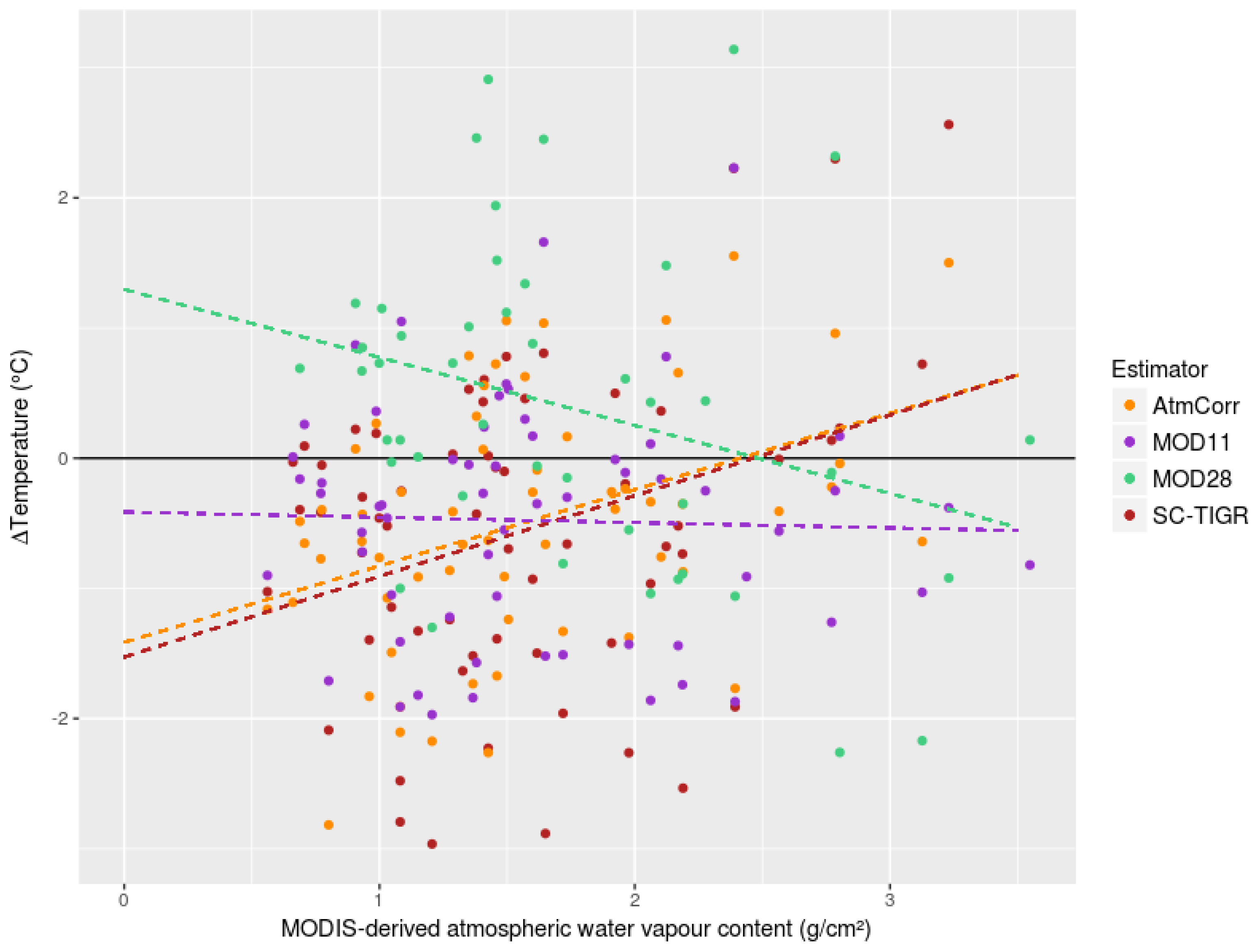
grid). For large lakes, this can be a problem when estimating the temperature for its whole surface and, considering the operational limitation of AtmCorr, MOD07L2 may be the best option when using Landsat imagery in these cases, since it provides water vapour content with spatial variability. The main issue with the estimates using MOD07L2 with the single-channel algorithm in our study is the lower accuracy in some SWT estimates, reaching out to a Δ T of ±3 ° C in some cases. Many of these low-quality estimates are consistent with the results found by Jiménez-Muñoz et al. [48], in which the error of the ST estimates increased considerably for atmospheric water vapour content higher than 3.0 g/cm 2 (Figure 6).
The performance found for MODIS also compared well with the literature, with both products showing performance similar to what was found in most studies [6,10,11,14,41]. Reinart and Reinhold [23] used MOD28 to estimate the LSWT of two large lakes in Sweden, and found a mean absolute difference of 0.41 ° C and r 2 of 0.993 for both lakes. In spite of the good performance found by the authors, LSWT estimates were compared with measured bulk temperatures, and so this may not be the case for the ST, since many of the data were from the summer months, when both lakes may have been thermally stratified.
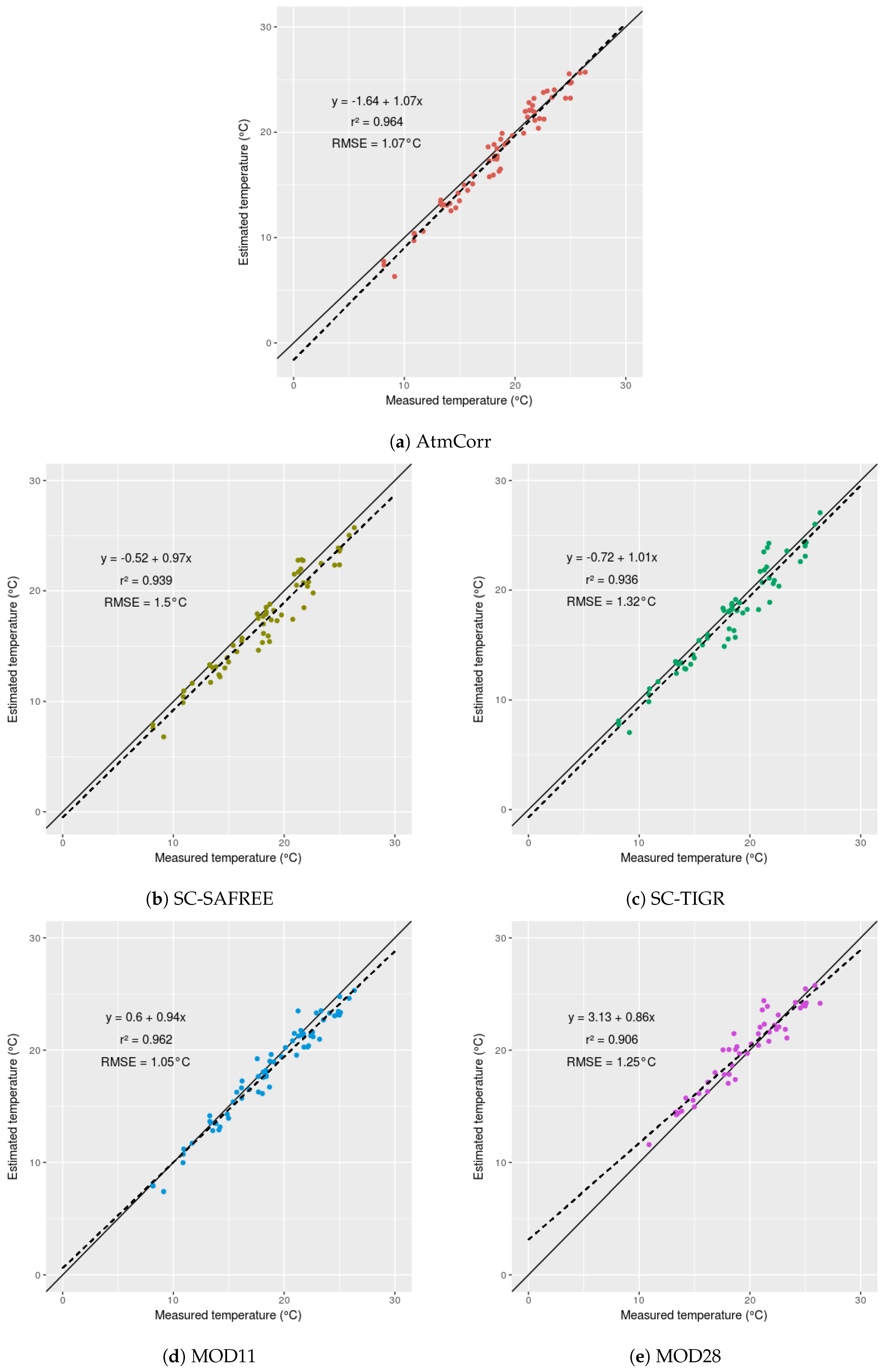
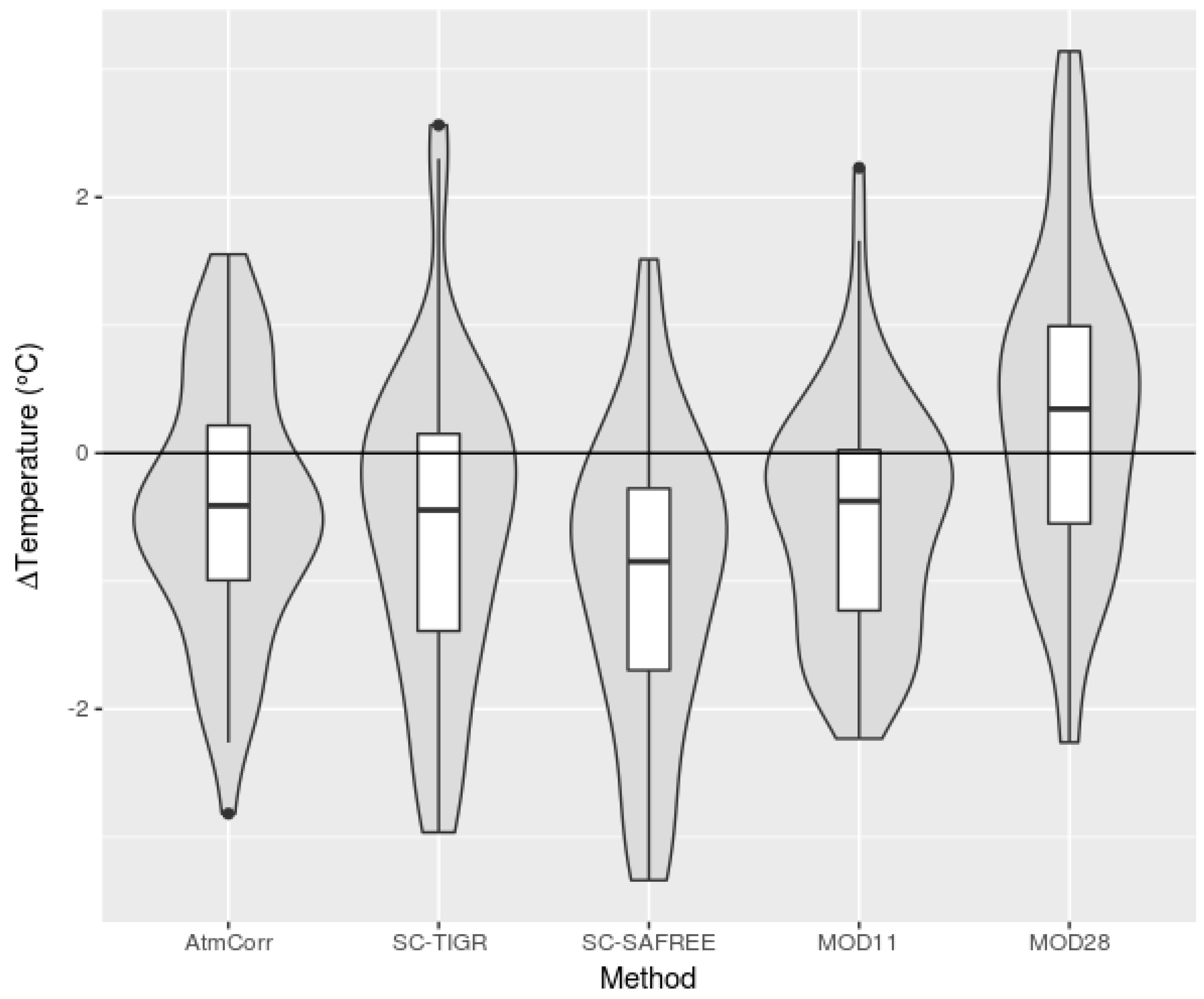
Our findings showed higher similarity between LSWT estimations based on MOD11, AtmCorr, and SC-TIGR, different from LSWT estimations based on MOD28. Despite the similar performance shown by MOD28 and SC-TIGR (in terms of absolute error and RMSE), MOD28 showed more erratic behavior, with a smaller correlation coefficient and different linear regression (Figure 4). Besides that, MOD28 showed a positive bias, while all other estimators showed a negative bias. Additionally, good agreement between the estimates using Landsat and MOD11 (Table 3 and Table 4) indicates that they are consistent estimators over this lake, while MOD28 is not, as there is a high correlation between the residuals for the Landsat methods and MOD11, but not between the former and MOD28. Even though high correlation was found between MOD11 and MOD28, it may be due to the fact that both MODIS products similarly overestimated small-to-medium temperatures and underestimated higher temperatures (despite MOD28 showing a positive bias), which was not observed in the Landsat estimates.
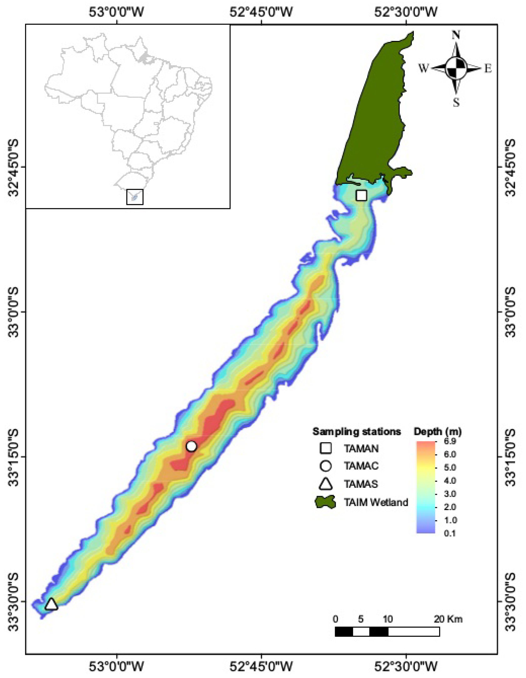
The lower performance obtained for MOD28 may be explained by its low spatial resolution of 4 km, which might be too coarse for Lake Mangueira due to its narrowness (5 km wide over the Northern station, and less than 4 km wide over the Southern station). In fact, errors in the estimates were considerably higher for the Southern station than for the Central and Northern stations, pointing to this. Considering that temperature varies more widely near the shores [6,8,24], it can be inferred that this product is not recommended for applications to lakes with narrow widths (in comparison to its spatial resolution), as is the case for Lake Mangueira.

4.2. Sensitivity to Parameters and Source of Errors

As seen in the literature, error in lake-water temperatures derived from remote-sensing imagery can occur mainly due to poor correction of atmospheric effects [30,71], water-surface effects [72], and due to the misrepresentation of water emissivity [30,45].
There is difficulty associated with estimating and removing atmospheric effects, which can promote substantial errors [31,70]. In fact, estimates tend to have lower accuracy when the water vapour content in the atmosphere is higher, since this increases the uncertainty regarding the effect of the atmosphere on the radiance measured by the sensor and, thus, in the correction parameters. Jiménez-Muñoz et al. [48] showed that the error in ST estimates considerably increased for atmospheric water vapour content higher than 3.0 g/cm 2 . Here, Landsat-derived estimates using AtmCorr showed a similar (although less pronounced) pattern. As atmospheric water vapour content (from the MOD07L2 water vapour product) increases, so does the error in the estimates of both SC-TIGR and AtmCorr, although this is not the case for MOD11 and MOD28 (Figure 6, Table 5). Although in other studies the accuracy of MODIS products decreased with higher temperatures (e.g., Reference [11]), which is related to higher water vapour content, this was not evident here (p-value > 0.05 for both products, Table 5). This may be due to the refined quality of the MODIS algorithm to remove these effects using its own band measurements [31], and to directly apply it in its ST products.
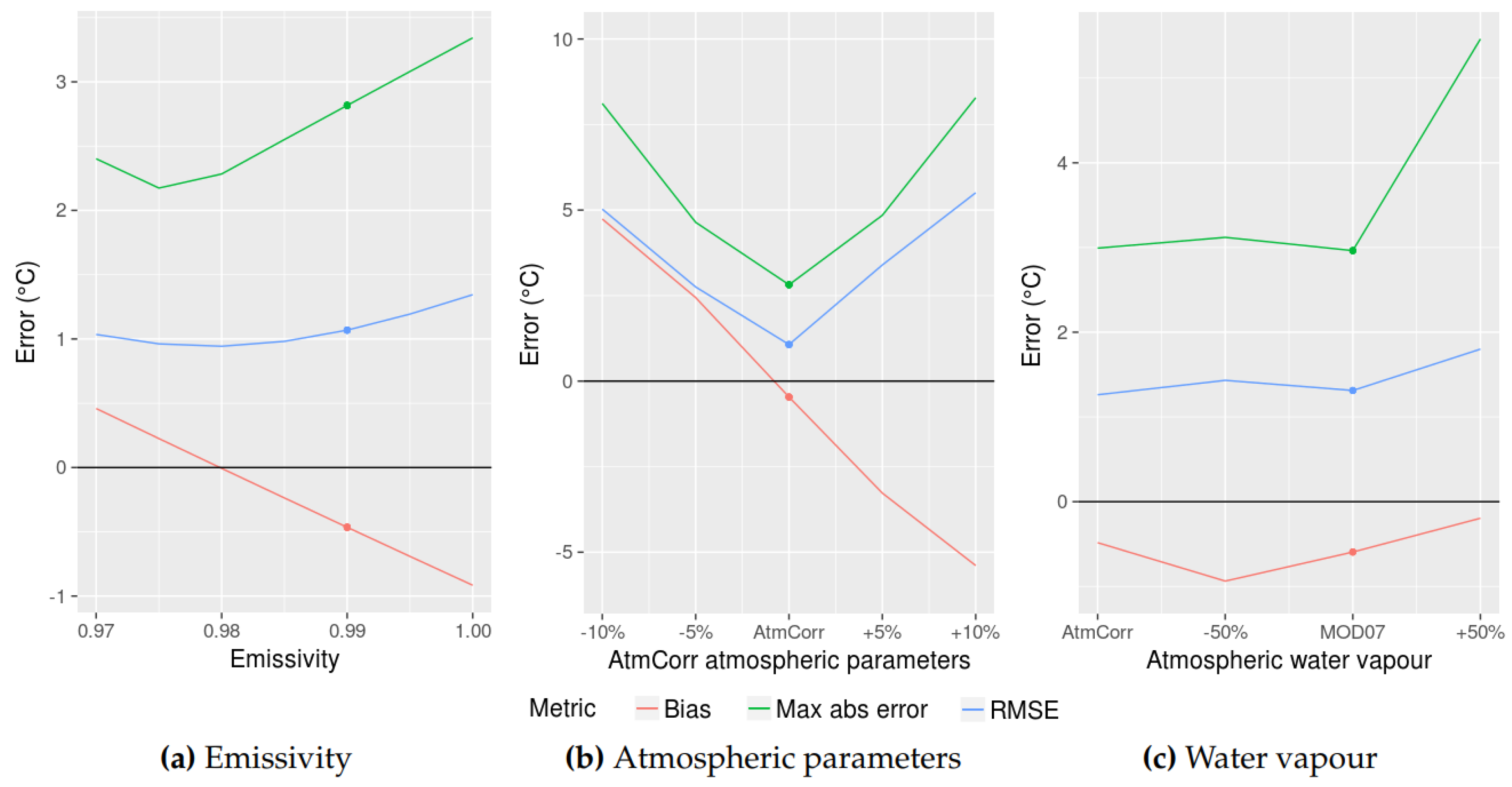
Temperature estimates using the RTE are very sensitive to atmospheric parameters (Figure 7), particularly to atmospheric transmissivity. For instance, a small change of 2.5% in atmospheric-transmissivity value implied an increase of about 2 ° C in the RMSE. The increase in errors is more pronounced when decreasing the values of the atmospheric parameters, showing that τ (which decreases as atmospheric water vapour increases) has a more important effect on L corr than L up and L down (both increase as atmospheric water vapour increases), which is expected considering Equation (6). In this case, negative bias also contributes to this sharp increase in errors, as it increased in magnitude when the atmospheric parameters negatively varied. This result highlights the importance of an accurate, precise source of estimation of the influence of the atmosphere on the radiance measured by the sensor, as has been shown in the literature by good results in estimation of LSWT when using in situ radiosonde data and radiative transfer models (e.g., Reference [12]).
The single-channel algorithm is much less sensitive to changes in atmospheric parameters, i.e., atmospheric water vapour content. Prats et al. [15] reported that a 50% decrease in water vapour content produced a decrease of 0.2–0.3 ° C in the estimated temperatures; in our sensitivity analysis, this decrease produced a (negative) increase of 0.3 ° C in the bias, and only marginally increased the RMSE (0.07 ° C). On the other hand, for increased w values, the RMSE and maximum error increased by 0.5 ° C and 1 ° C, respectively, which is consistent with the report of Jiménez-Muñoz et al. [48]. Considering the small size (in comparison to emissivity and the radiance measured by the sensor) of the contribution of the water vapour content to the temperature estimates in this algorithm, MOD07L2 can be used for retrievals of LSWT using Landsat images, since data are measured daily and are spatially distributed, and this product is ready to use.
In our study, only a few estimates were made when water vapour content was high (>3 g/cm 2 , Figure 6), which limits further understanding of the performance of these methods under such conditions. However, as seen in these few estimates and in the literature (e.g., References [11,48]), studies estimating LSWT in areas with high atmospheric water vapour, such as tropical areas, should keep in mind that estimation is bound to produce higher errors, especially when using Landsat imagery (Table 8). For the Landsat methods, other sources of atmospheric parameters, such as reanalysis products [15,31], should also be further studied in order to be used with the radiative transfer equation in an effort to increase the accuracy of the estimates.
The cool bias found in our study was also found in most LSWT studies (e.g., References [6,10,11,15,73]). This can be a result of the cool-skin effect, when the few millimetres at the top of the water column are colder than the water underneath. Usually, this is not measured by in situ sensors but affects estimates made using remote sensing [74]. The cool-skin effect reduces water temperature over a range of 0.1–0.6 ° C, occurring as a result of heat loss from water to air due to evaporation, and is affected mainly by wind speed [72,75]. A warm-layer effect can also be observed during calm sunny days in deeper lakes, where thermal stratification can occur, and can increase the ST up to several degrees [76], but as observed here and in other studies (e.g., Reference [36]), this is not the case for the shallow Lake Mangueira.
While this effect is different for each lake and depends on in situ lake-temperature measurements to be understood, techniques are available to address the cool-skin effect in sea water, which assume this to be a function of wind speed [75]. Although we did not attempt to assess and remove the cool-skin effect in the estimations here, our study shows that it is important in LSWT studies using remote sensing. Prats et al. [15] estimated the LSWT for French water bodies for a long time series using Landsat 5 TM and 7 ETM+ images, applying an adjusted sea-water algorithm to remove the effects of the cool-skin and warm-layer effects, and testing these approaches on a reservoir with in situ data to validate it. The estimated cool-skin effect reduced the LSWT by about 0.3 to 0.6 ° C for most of the data, and even though the authors concluded that the algorithm required further adaptations for use on continental waters, it demonstrated how techniques to remove these effects can be useful to improve the accuracy of remote sensing-derived SWT in lake studies.
In the case of emissivity, considering that MODIS products use a fixed value of emissivity for water, as was also used in our study for Landsat 7 ETM+ images (as well as in most studies of water-temperature estimations using remote sensing, e.g., References [15,24]), it can also be a source of considerable error. Emissivity varies with several parameters, such as salinity and turbidity, which can result in errors of estimation ranging from 0.2 to 0.5 ° C [45]. Hulley et al. [32] used an algorithm to improve the estimation of water emissivity and the coefficients for the split-window algorithm for MOD11, in order to improve its estimation of inland SWT. They found differences of emissivity in up to 0.01 for MODIS, which resulted in errors of 0.3–0.7 ° C.
As shown in the sensitivity analysis, emissivity has a significant impact on the estimated temperatures, and showed an optimal value of 0.98, reducing the RMSE and maximum absolute error by 10% and 20%, respectively, compared to our standard value of 0.99. This, however, can be a result of the balancing of the cool-skin effect: as the latter reduces water temperature at the surface, a lower value of emissivity (i.e., further from its physical, more-likely value) makes the surface appear warmer than it is, partially compensating for the cool-skin effect. Although this 0.98 emissivity value produced the best results, we assumed (taking into account that it was not measured) that the closest value, from 0.97 to 1, to its real value is 0.99, which was calculated by Masuda et al. [69] and also found in MODIS product MOD11 (0.992 for band 31 and 0.988 for band 32) for Lake Mangueira. Due to the limitation of water emissivity estimation [66], most approaches still use a fixed, tabulated value of emissivity, found in reflectivity and emissivity data available in spectral libraries such as MODIS’ [77]. As emissivity and the removal of the cool-skin effect are limiting factors to be improved in LSWT estimations, the use of lower emissivity values can be tested in future studies to reduce errors resulting from the latter in an effort to improve the accuracy of LSWT estimates.

5. Conclusions

In this study, we compared different methods for estimating lake-surface-water temperatures using Landsat 7 ETM+ and MODIS products. Considering the results from our study and the literature, MOD11 is the recommended product to be used in LSWT studies due to its accuracy (values of bias, RMSE, and r 2 of −0.523 ° C, 1.05 ° C and 0.962, respectively), temporal resolution, and ease of use, and should be preferred over MOD28, which gave less accurate results. Landsat 7 ETM+ should be used in small lakes, due to its higher spatial resolution, and we recommend the application of the radiative transfer equation with atmospheric correction parameters when possible. Despite its high sensitivity to these parameters, as shown in our work, which can result in gross errors in temperature estimates, this equation was successfully applied in Lake Mangueira with AtmCorr, and showed quite similar performance to MOD11 (values of bias, RMSE, and r 2 of −0.465 ° C, 1.07 ° C, and 0.964, respectively). The limitations of this application are difficulties in operating this platform, and that it only provides correction parameters for a point (i.e., it is not spatially distributed). Although not as accurate, the single-channel algorithm can also be used with Landsat imagery using the TIGR3 database, and most sources of atmospheric water-vapour content, since it is not very sensitive to this parameter. We recommend MOD07L2 to be used with this algorithm, because the data are measured daily and spatially distributed, and it is ready to use. However, users should take into account that the accuracy of this algorithm is considerably reduced in cases when atmospheric water vapour content is high.
We recommend that similar tests be done for Landsat imagery (especially on RTE sensitivity to different sources of atmospheric parameters) on other lakes with different geographical and morphological characteristics to support our findings. We also recommend the further development and adaptation of techniques to assess and remove the cool-skin effect in SWT estimations in inland waters to reduce the cool bias seen in most studies on this subject, and tests of different emissivity values, to verify if they can compensate, to some degree, for the cool-skin effect, in an effort to improve the accuracy of these estimates.

Supplementary Materials

The following are available online at https://www.mdpi.com/2073-4441/11/1/168/s1, Table S1: Days with temperature measurements considered in this study, along with the Landsat 7 ETM+ and MODIS images available for each date.

Author Contributions

Conceptualization, M.H.T. and D.M.-M.; methodology, M.H.T., A.H.F.C., and A.L.R.; validation, M.H.T., A.L.R., C.R.F.J.; formal analysis, M.H.T.; investigation, M.H.T. and A.H.F.C.; data curation, M.H.T. and A.M.M.; writing—original draft preparation, M.H.T. and D.M.-M.; writing—review and editing, A.H.F.C., A.L.R., J.R.C., C.R.F.J., J.M.B., A.M.M., F.M.F., and L.H.R.R.; visualization, J.M.B., F.M.F., and L.H.R.R.; supervision, D.M.-M., C.R.F.J., J.R.C., and A.L.R.; funding acquisition, D.M.-M.

Funding

This paper was funded by CAPES (Coordenação de Aperfeiçoamento de Pessoal de Nível Superior) through a research grant to Matheus Henrique Tavares and the project “Qualidade e circulação de água em ecossistemas costeiros: monitoramento e modelagem para tomada de decisão”, and CNPq (Conselho Nacional de Desenvolvimento Científico e Tecnológico) through a research grant to Augusto Hugo Farias da Cunha and the project entitled “Impacto das mudanças climáticas em ambientes fluviais e lacustres do Rio Grande do Sul”.

Acknowledgments

We would like to thank the three anonymous reviewers for their contributions, which greatly improved this paper, Julia Barsi from NASA for helping with automating AtmCorr, and the Global Lake Ecological Observatory Network (GLEON) for providing resources and a venue for the discussion on lakes.

Conflicts of Interest

The authors declare no conflict of interest. The funders had no role in the design of the study; in the collection, analyses, or interpretation of data; in the writing of the manuscript; or in the decision to publish the results.

References

  1. Horne, A.J.; Goldman, C.R. Limnology; McGraw-Hill: New York, NY, USA, 1994. [Google Scholar]
  2. Adrian, R.; O’Reilly, C.M.; Zagarese, H.; Baines, S.B.; Hessen, D.O.; Keller, W.; Livingstone, D.M.; Sommaruga, R.; Straile, D.; Donk, E.V.; et al. Lakes as sentinels of climate change. Lymnol. Oceanogr. 2009, 54, 2283–2297. [Google Scholar] [CrossRef] [Green Version]
  3. O’Reilly, C.M.; Sharma, S.; Gray, D.K.; Hampton, S.E.; Read, J.S.; Rowley, R.J.; Schneider, P.; Lenters, J.D.; McIntyre, P.B.; Kraemer, B.M.; et al. Rapid and highly variable warming of lake surface waters around the globe. Geophys. Res. Lett. 2015, 42, 10–773. [Google Scholar] [CrossRef]
  4. Yang, K.; Yu, Z.; Luo, Y.; Yang, Y.; Zhao, L.; Zhou, X. Spatial and temporal variations in the relationship between lake water surface temperatures and water quality—A case study of Dianchi Lake. Sci. Total Environ. 2018, 624, 859–871. [Google Scholar] [CrossRef] [PubMed]
  5. Kay, J.E.; Kampf, S.K.; Handcock, R.N.; Cherkauer, K.A.; Gillespie, A.R.; Burges, S.J. Accuracy of lake and stream temperatures estimated from thermal infrared images. JAWRA J. Am. Water Resour. Assoc. 2005, 41, 1161–1175. [Google Scholar] [CrossRef]
  6. Crosman, E.T.; Horel, J.D. MODIS-derived surface temperature of the Great Salt Lake. Remote Sens. Environ. 2009, 113, 73–81. [Google Scholar] [CrossRef]
  7. Handcock, R.; Gillespie, A.; Cherkauer, K.; Kay, J.; Burges, S.; Kampf, S. Accuracy and uncertainty of thermal-infrared remote sensing of stream temperatures at multiple spatial scales. Remote Sens. Environ. 2006, 100, 427–440. [Google Scholar] [CrossRef]
  8. Alcântara, E.H.; Stech, J.L.; Lorenzzetti, J.A.; Bonnet, M.P.; Casamitjana, X.; Assireu, A.T.; de Moraes Novo, E.M.L. Remote sensing of water surface temperature and heat flux over a tropical hydroelectric reservoir. Remote Sens. Environ. 2010, 114, 2651–2665. [Google Scholar] [CrossRef]
  9. Curtarelli, M.; Alcântara, E.; Rennó, C.; Stech, J. Effects of cold fronts on MODIS-derived sensible and latent heat fluxes in Itumbiara reservoir (Central Brazil). Adv. Space Res. 2013, 52, 1668–1677. [Google Scholar] [CrossRef]
  10. Sima, S.; Ahmadalipour, A.; Tajrishy, M. Mapping surface temperature in a hyper-saline lake and investigating the effect of temperature distribution on the lake evaporation. Remote Sens. Environ. 2013, 136, 374–385. [Google Scholar] [CrossRef]
  11. Liu, G.; Ou, W.; Zhang, Y.; Wu, T.; Zhu, G.; Shi, K.; Qin, B. Validating and mapping surface water temperatures in Lake Taihu: Results from MODIS land surface temperature products. IEEE J. Sel. Top. Appl. Earth Obs. Remote Sens. 2015, 8, 1230–1244. [Google Scholar] [CrossRef]
  12. Allan, M.G.; Hamilton, D.P.; Trolle, D.; Muraoka, K.; McBride, C. Spatial heterogeneity in geothermally-influenced lakes derived from atmospherically corrected Landsat thermal imagery and three-dimensional hydrodynamic modelling. Int. J. Appl. Earth Obs. Geoinf. 2016, 50, 106–116. [Google Scholar] [CrossRef]
  13. Ling, F.; Foody, G.M.; Du, H.; Ban, X.; Li, X.; Zhang, Y.; Du, Y. Monitoring Thermal Pollution in Rivers Downstream of Dams with Landsat ETM+ Thermal Infrared Images. Remote Sens. 2017, 9, 1175. [Google Scholar] [CrossRef]
  14. Pareeth, S.; Salmaso, N.; Adrian, R.; Neteler, M. Homogenised daily lake surface water temperature data generated from multiple satellite sensors: A long-term case study of a large sub-Alpine lake. Sci. Rep. 2016, 6, 31251. [Google Scholar] [CrossRef] [PubMed] [Green Version]
  15. Prats, J.; Reynaud, N.; Rebière, D.; Peroux, T.; Tormos, T.; Danis, P.A. LakeSST: Lake Skin Surface Temperature in French inland water bodies for 1999–2016 from Landsat archives. Earth Syst. Sci. Data 2018, 10, 727–743. [Google Scholar] [CrossRef] [Green Version]
  16. Luz, G.A.; Guasselli, L.A.; Rocha, D. Temperature Surface of Guaíba Lake, RS, from time series of MODIS images. Braz. J. Water Resour. 2017, 22. [Google Scholar] [CrossRef] [Green Version]
  17. Schneider, P.; Hook, S.J. Space observations of inland water bodies show rapid surface warming since 1985. Geophys. Res. Lett. 2010, 37. [Google Scholar] [CrossRef] [Green Version]
  18. Woolway, R.I.; Merchant, C.J. Intralake heterogeneity of thermal responses to climate change: A study of large Northern Hemisphere lakes. J. Geophys. Res. Atmos. 2018, 123, 3087–3098. [Google Scholar] [CrossRef]
  19. Jiménez-Muñoz, J.C.; Sobrino, J.A. A generalized single-channel method for retrieving land surface temperature from remote sensing data. J. Geophys. Res. 2003, 108, D22. [Google Scholar] [CrossRef]
  20. Li, Z.L.; Tang, B.H.; Wu, H.; Ren, H.; Yan, G.; Wan, Z.; Trigo, I.F.; Sobrino, J.A. Satellite-derived land surface temperature: Current status and perspectives. Remote Sens. Environ. 2013, 131, 14–37. [Google Scholar] [CrossRef] [Green Version]
  21. Weng, Q.; Fu, P.; Gao, F. Generating daily land surface temperature at Landsat resolution by fusing Landsat and MODIS data. Remote Sens. Environ. 2014, 145, 55–67. [Google Scholar] [CrossRef]
  22. Kilpatrick, K.; Podestá, G.; Walsh, S.; Williams, E.; Halliwell, V.; Szczodrak, M.; Brown, O.; Minnett, P.; Evans, R. A decade of sea surface temperature from MODIS. Remote Sens. Environ. 2015, 165, 27–41. [Google Scholar] [CrossRef]
  23. Reinart, A.; Reinhold, M. Mapping surface temperature in large lakes with MODIS data. Remote Sens. Environ. 2008, 112, 603–611. [Google Scholar] [CrossRef]
  24. Lamaro, A.A.; Mariñelarena, A.; Torrusio, S.E.; Sala, S.E. Water surface temperature estimation from Landsat 7 ETM+ thermal infrared data using the generalized single-channel method: Case study of Embalse del Río Tercero (Córdoba, Argentina). Adv. Space Res. 2013, 51, 492–500. [Google Scholar] [CrossRef]
  25. Barnes, W.L.; Pagano, T.S.; Salomonson, V.V. Prelaunch characteristics of the Moderate Resolution Imaging Spectroradiometer (MODIS) on EOS-AM1. IEEE Trans. Geosci. Remote Sens. 1998, 36, 1088–1100. [Google Scholar] [CrossRef] [Green Version]
  26. Barsi, J.A.; Schott, J.; Palluconi, F.D.; Helder, D.L.; Hook, S.J.; Markham, B.L.; Chander, G.; O’Donnell, E.M. Landsat TM and ETM+ thermal band calibration. Can. J. Remote Sens. 2003, 29, 141–153. [Google Scholar] [CrossRef] [Green Version]
  27. Gholizadeh, M.; Melesse, A.; Reddi, L. A comprehensive review on water quality parameters estimation using remote sensing techniques. Sensors 2016, 16, 1298. [Google Scholar] [CrossRef] [PubMed]
  28. Schneider, K.; Mauser, W. Processing and accuracy of Landsat Thematic Mapper data for lake surface temperature measurement. Int. J. Remote Sens. 1996, 17, 2027–2041. [Google Scholar] [CrossRef]
  29. Ruiz-Verdú, A.; Jiménez, J.C.; Lazzaro, X.; Tenjo, C.; Delegido, J.; Pereira, M.; Sobrino, J.A.; Moreno, J. Comparison of MODIS and Landsat-8 retrievals of chlorophyll-a and water temperature over Lake Titicaca. In Proceedings of the 2016 IEEE Geoscience and Remote Sensing Symposium (IGARSS’16), Beijing, China, 10–15 July 2016; pp. 7643–7646. [Google Scholar]
  30. Jiménez-Muñoz, J.; Sobrino, J. Error sources on the land surface temperature retrieved from thermal infrared single channel remote sensing data. Int. J. Remote Sens. 2006, 27, 999–1014. [Google Scholar] [CrossRef]
  31. Jiménez-Muñoz, J.C.; Sobrino, J.A.; Mattar, C.; Franch, B. Atmospheric correction of optical imagery from MODIS and Reanalysis atmospheric products. Remote Sens. Environ. 2010, 114, 2195–2210. [Google Scholar] [CrossRef]
  32. Hulley, G.C.; Hook, S.J.; Schneider, P. Optimized split-window coefficients for deriving surface temperatures from inland water bodies. Remote Sens. Environ. 2011, 115, 3758–3769. [Google Scholar] [CrossRef]
  33. Yu, X.; Guo, X.; Wu, Z. Land surface temperature retrieval from Landsat 8 TIRS–Comparison between radiative transfer equation-based method, split window algorithm and single channel method. Remote Sens. 2014, 6, 9829–9852. [Google Scholar] [CrossRef]
  34. Fricke, K.; Baschek, B. Water surface temperature profiles for the Rhine River derived from Landsat ETM+ data. Proc. SPIE 2013, 88870E. [Google Scholar] [CrossRef]
  35. Simon, R.; Tormos, T.; Danis, P.A. Retrieving water surface temperature from archive LANDSAT thermal infrared data: Application of the mono-channel atmospheric correction algorithm over two freshwater reservoirs. Int. J. Appl. Earth Obs. Geoinf. 2014, 30, 247–250. [Google Scholar] [CrossRef]
  36. Fragoso, C.R., Jr.; Marques, D.M.M.; Ferreira, T.F.; Janse, J.H.; van Nes, E.H. Potential effects of climate change and eutrophication on a large subtropical shallow lake. Environ. Model. Softw. 2011, 26, 1337–1348. [Google Scholar] [CrossRef]
  37. Crossetti, L.O.; Becker, V.; de Souza Cardoso, L.; Rodrigues, L.R.; da Costa, L.S.; Motta-Marques, D. Is phytoplankton functional classification a suitable tool to investigate spatial heterogeneity in a subtropical shallow lake? Limnol. Ecol. Manag. Inland Waters 2013, 43, 157–163. [Google Scholar] [CrossRef]
  38. Kottek, M.; Grieser, J.; Beck, C.; Rudolf, B.; Rubel, F. World map of the Köppen-Geiger climate classification updated. Meteorol. Z. 2006, 15, 259–263. [Google Scholar] [CrossRef]
  39. Woolway, R.I.; Jones, I.D.; Maberly, S.C.; French, J.R.; Livingstone, D.M.; Monteith, D.T.; Simpson, G.L.; Thackeray, S.J.; Andersen, M.R.; Battarbee, R.W.; et al. Diel surface temperature range scales with lake size. PLoS ONE 2016, 11, e0152466. [Google Scholar] [CrossRef] [PubMed]
  40. Munar, A.M. Pareamento Bacia-Lagoa Usando Modelagem HidrolóGica-HidrodinâMica E Sensoriamento Remoto. Ph.D. Thesis, Postgraduate Program in Water Resources and Environmental Sanitation, Federal University of Rio Grande do Sul, Porto Alegre, Rio Grande do Sul, Brazil, 2017; 139p. [Google Scholar]
  41. Chavula, G.; Brezonik, P.; Thenkabail, P.; Johnson, T.; Bauer, M. Estimating the surface temperature of Lake Malawi using AVHRR and MODIS satellite imagery. Phys. Chem. Earth Parts A/B/C 2009, 34, 749–754. [Google Scholar] [CrossRef]
  42. Zhang, Q.; Ye, X.C.; Werner, A.D.; Li, Y.L.; Yao, J.; Li, X.H.; Xu, C.Y. An investigation of enhanced recessions in Poyang Lake: comparison of Yangtze River and local catchment impacts. J. Hydrol. 2014, 517, 425–434. [Google Scholar] [CrossRef]
  43. Cavalcanti, J.R.; da Motta-Marques, D.M.L.; Fragoso, C.R., Jr. Process-based modeling of shallow lake metabolism: Spatio-temporal variability and relative importance of individual processes. Ecol. Model. 2016, 323, 28–40. [Google Scholar] [CrossRef]
  44. Wan, Z.; Dozier, J. A generalized split-window algorithm for retrieving land-surface temperature from space. IEEE Trans. Geosci. Remote Sens. 1996, 34, 892–905. [Google Scholar]
  45. Friedman, D. Infrared characteristics of ocean water (1.5–15 μ). Appl. Opt. 1969, 8, 2073–2078. [Google Scholar] [CrossRef] [PubMed]
  46. Walton, C.; Pichel, W.; Sapper, J.; May, D. The development and operational application of nonlinear algorithms for the measurement of sea surface temperatures with the NOAA polar-orbiting environmental satellites. J. Geophys. Res. Oceans 1998, 103, 27999–28012. [Google Scholar] [CrossRef] [Green Version]
  47. Schott, J.R. Remote Sensing: The Image Chain Approach, 2nd ed.; Oxford University Press: Oxford, UK, 2007. [Google Scholar]
  48. Jiménez-Muñoz, J.C.; Cristobal, J.; Sobrino, J.A.; Soria, G.; Ninyerola, M.; Pons, X.; Pons, X. Revision of the Single-Channel Algorithm for Land Surface Temperature Retrieval From Landsat Thermal-Infrared Data. IEEE Trans. Geosci. Remote Sens. 2009, 47, 339–349. [Google Scholar] [CrossRef]
  49. Cristóbal, J.; Jiménez-Muñoz, J.C.; Sobrino, J.A.; Ninyerola, M.; Pons, X. Improvements in land surface temperature retrieval from the Landsat series thermal band using water vapor and air temperature. J. Geophys. Res. 2009, 114, D08103. [Google Scholar] [CrossRef]
  50. Díaz-Delgado, R.; Ameztoy, I.; Cristóbal, J.; Bustamante, J. Long time series of Landsat images to reconstruct river surface temperature and turbidity regimes of Guadalquivir Estuary. In Proceedings of the 2010 IEEE Geoscience and Remote Sensing Symposium (IGARSS’10), Honolulu, HI, USA, 25–30 July 2010; pp. 233–236. [Google Scholar]
  51. Barsi, J.A.; Barker, J.L.; Schott, J.R. An atmospheric correction parameter calculator for a single thermal band earth-sensing instrument. In Proceedings of the 2003 IEEE Geoscience and Remote Sensing Symposium (IGARSS’03), Toulouse, France, 21–25 July 2003; Volume 5, pp. 3014–3016. [Google Scholar]
  52. Barsi, J.A.; Schott, J.; Palluconi, F.D.; Hook, S.J. Validation of a Web-Based Atmospheric Correction Tool for Single Thermal Band Instruments. Earth Obs. Syst. X Int. Soc. Opt. Photonics 2005, 5882, 58820E. [Google Scholar]
  53. Sobrino, J.A.; Raissouni, N. Toward remote sensing methods for land cover dynamic monitoring: Application to Morocco. Int. J. Remote Sens. 2000, 21, 353–366. [Google Scholar] [CrossRef]
  54. Okwen, R.; Pu, R.; Cunningham, J. Remote sensing of temperature variations around major power plants as point sources of heat. Int. J. Remote Sens. 2011, 32, 3791–3805. [Google Scholar] [CrossRef]
  55. Deng, C.; Wu, C. Examining the impacts of urban biophysical compositions on surface urban heat island: A spectral unmixing and thermal mixing approach. Remote Sens. Environ. 2013, 131, 262–274. [Google Scholar] [CrossRef]
  56. Chander, G.; Markham, B.L.; Helder, D.L. Summary of current radiometric calibration coefficients for Landsat MSS, TM, ETM+, and EO-1 ALI sensors. Remote Sens. Environ. 2009, 113, 893–903. [Google Scholar] [CrossRef] [Green Version]
  57. R Core Team. R: A Language and Environment for Statistical Computing; R Foundation for Statistical Computing: Vienna, Austria, 2017. [Google Scholar]
  58. Bivand, R.; Lewin-Koh, N. Maptools: Tools for Reading and Handling Spatial Objects; R Package Version 0.9-2; R Foundation for Statistical Computing: Vienna, Austria, 2017. [Google Scholar]
  59. Pebesma, E.J.; Bivand, R.S. Classes and methods for spatial data in R. R News 2005, 5, 9–13. [Google Scholar]
  60. Hijmans, R.J. Raster: Geographic Data Analysis and Modeling; R Package Version 2.6-7; R Foundation for Statistical Computing: Vienna, Austria, 2017. [Google Scholar]
  61. Bivand, R.; Keitt, T.; Rowlingson, B. rgdal: Bindings for the ’Geospatial’ Data Abstraction Library, R package version 1.2-15; R Foundation for Statistical Computing: Vienna, Austria, 2017. [Google Scholar]
  62. Bivand, R.; Rundel, C. rgeos: Interface to Geometry Engine - Open Source (’GEOS’), R package version 0.3-26; R Foundation for Statistical Computing: Vienna, Austria, 2017. [Google Scholar]
  63. Mao, K.; Qin, Z.; Shi, J.; Gong, P. A practical split-window algorithm for retrieving land-surface temperature from MODIS data. Int. J. Remote Sens. 2005, 26, 3181–3204. [Google Scholar] [CrossRef]
  64. Sobrino, J.A.; Jiménez-Muñoz, J.C.; Paolini, L. Land surface temperature retrieval from LANDSAT TM 5. Remote Sens. Environ. 2004, 90, 434–440. [Google Scholar] [CrossRef]
  65. Sobrino, J.A.; Jiménez-Muñoz, J.C.; Soria, G.; Romaguera, M.; Guanter, L.; Moreno, J.; Plaza, A.; Martinez, P. Land Surface Emissivity Retrieval From Different VNIR and TIR Sensors. IEEE Trans. Geosci. Remote Sens. 2008, 46, 316–327. [Google Scholar] [CrossRef]
  66. Handcock, R.N.; Torgersen, C.E.; Cherkauer, K.A.; Gillespie, A.R.; Tockner, K.; Faux, R.N.; Tan, J. Thermal infrared remote sensing of water temperature in riverine landscapes. In Fluvial Remote Sensing for Science and Management; Wiley: Hoboken, NJ, USA, 2012; pp. 85–113. [Google Scholar]
  67. Wloczyk, C.; Richter, R.; Borg, E.; Neubert, W. Sea and lake surface temperature retrieval from Landsat thermal data in Northern Germany. Int. J. Remote Sens. 2006, 27, 2489–2502. [Google Scholar] [CrossRef]
  68. Snyder, W.C.; Wan, Z.; Zhang, Y.; Feng, Y.Z. Classification-based Emissivity for Land Surface Temperature Measurement from Space. Int. J. Remote Sens. 1998, 19, 2753–2774. [Google Scholar] [CrossRef]
  69. Masuda, K.; Takashima, T.; Takayama, Y. Emissivity of pure and sea waters for the model sea surface in the infrared window regions. Remote Sens. Environ. 1988, 24, 313–329. [Google Scholar] [CrossRef]
  70. Coll, C.; Caselles, V.; Valor, E.; Niclòs, R. Comparison between different sources of atmospheric profiles for land surface temperature retrieval from single channel thermal infrared data. Remote Sens. Environ. 2012, 117, 199–210. [Google Scholar] [CrossRef]
  71. Harris, A.; Mason, I. An extension to the split-window technique giving improved atmospheric correction and total water vapour. Int. J. Remote Sens. 1992, 13, 881–892. [Google Scholar] [CrossRef]
  72. Robinson, I.; Wells, N.; Charnock, H. The sea surface thermal boundary layer and its relevance to the measurement of sea surface temperature by airborne and spaceborne radiometers. Int. J. Remote Sens. 1984, 5, 19–45. [Google Scholar] [CrossRef]
  73. MacCallum, S.N.; Merchant, C.J. Surface water temperature observations of large lakes by optimal estimation. Can. J. Remote Sens. 2012, 38, 25–45. [Google Scholar] [CrossRef]
  74. Schluessel, P.; Emery, W.J.; Grassl, H.; Mammen, T. On the bulk-skin temperature difference and its impact on satellite remote sensing of sea surface temperature. J. Geophys. Res. Oceans 1990, 95, 13341–13356. [Google Scholar] [CrossRef]
  75. Fairall, C.; Bradley, E.F.; Godfrey, J.; Wick, G.; Edson, J.B.; Young, G. Cool-skin and warm-layer effects on sea surface temperature. J. Geophys. Res. Oceans 1996, 101, 1295–1308. [Google Scholar] [CrossRef]
  76. Ward, B. Near-surface ocean temperature. J. Geophys. Res. Oceans 2006, 111. [Google Scholar] [CrossRef] [Green Version]
  77. Zhang, Y. MODIS UCSB Emissivity Library. 1999. Available online: https://icess.eri.ucsb.edu/modis/EMIS/html/em.html (accessed on 5 December 2018).
Figure 1. Map of Lake Mangueira, showing the three stations, Northern (TAMAN), Central (TAMAC) and Southern (TAMAS). (Source: Munar [40]).
Water 11 00168 g001
Figure 2. Flowchart illustrating the procedure used to estimate lake-surface-water temperature (LSWT) using Landsat 7 ETM+ and MODIS imagery to compare with measured data.
Water 11 00168 g002
Figure 3. Measured temperatures in the three stations across Lake Mangueira from 2001 to 2018, plotted according to the day of the year. Summer starts on day 356 and ends on day 80, and winter starts on day 173 and ends on day 266.
Water 11 00168 g003
Figure 4. Comparison of the in situ measured LSWT with the temperatures estimated by each method using Landsat 7 ETM+ imagery with the RTE and AtmCorr (a) and with the single-channel algorithm (b,c), and using MODIS products MOD11 (d) and MOD28 (e).
Water 11 00168 g004
Figure 5. Boxplot and violin plot of the residuals between the temperatures estimated by each method and the measured temperatures.
Water 11 00168 g005
Figure 6. Comparison of the residuals found for estimations using Landsat 7 ETM+ and MODIS with atmospheric water vapour content estimated by MOD07L2. The dashed lines represent the linear regression between Δ T and w for each method (values are in Table 5).
Water 11 00168 g006
Figure 7. Sensitivity analysis of the estimated LSWT to (a) emissivity, (b) atmospheric parameters, and (c) water vapour content, showing the resulting bias, absolute maximum error, and RMSE when varying them, for (a) from 0.97 to 1.0, for (b) from −10% to +10% (−5% to +5% for atmospheric transmissivity), and for (c) from −50% to +50%, taking MOD07L2 as reference. The dots represent the values employed in this work.
Water 11 00168 g007
Table 1. Nomenclature of methods used for the estimation of LSWT using Landsat 7 ETM+ imagery. Note: AtmCorr, NASA’s Atmospheric Correction Parameter Calculator.
MethodDescription
AtmCorrRadiative transfer equation applied with atmospheric correction parameters from AtmCorr
SC-SAFREESingle-channel algorithm using SAFREE database and MOD07L2’s water vapour
SC-TIGRSingle-channel algorithm using TIGR3 database and MOD07L2’s water vapour
Table 2. Metrics calculated for each method of estimating Lake Mangueira’s SWT using Landsat 7 ETM+ imagery and MODIS products.
MethodAbsolute Error ( ° C)Bias ( ° C)RMSE ( ° C) r 2
AtmCorr0.880−0.4651.070.964
SC-SAFREE1.19−0.9901.500.936
SC-TIGR1.00−0.5601.320.938
MOD110.825−0.5231.050.962
MOD280.9890.3291.250.906
Table 3. p-value of the Tukey’s test between the residuals of each method.
MethodAtmCorrSC-TIGRSC-SAFREEMOD11MOD28
AtmCorrNA0.967<0.050.990<0.05
SC-TIGR0.967NA0.1980.999<0.05
SC-SAFREE<0.050.198NA0.113<0.05
MOD110.9900.9990.113NA<0.05
MOD28<0.05<0.05<0.05<0.05NA
Table 4. Correlation coefficient between the residuals of each method.
MethodAtmCorrSC-TIGRSC-SAFREEMOD11MOD28
AtmCorrNA0.7680.7300.6060.355
SC-TIGR0.768NA0.9620.6700.324
SC-SAFREE0.7300.962NA0.7040.425
MOD110.6700.6060.496NA0.644
MOD280.3240.3550.4250.644NA
Table 5. p-value of the linear regression between the residuals and w for each method.
MethodSlopeInterceptp-Value
AtmCorr0.587−1.41<0.01
SC-TIGR0.620−1.53<0.01
MOD11−0.041−0.4130.813
MOD28−0.5221.300.0513
Table 6. Metrics calculated for sensitivity analysis of the temperature estimates to emissivity.
EmissivityBias ( ° C)RMSE ( ° C)Maximum Error ( ° C) r 2
1.00−0.9161.34−3.340.965
0.995−0.6911.19−3.080.965
0.990 *−0.4651.07−2.820.965
0.985−0.2370.981−2.550.965
0.980−0.00680.943−2.280.965
0.9750.2250.9622.170.965
0.9700.4591.042.400.965
* value of emissivity used in this study.
Table 7. Metrics calculated for sensitivity analysis of the temperature estimates to atmospheric parameters.
Atmospheric ParametersBias ( ° C)RMSE ( ° C)Maximum Error ( ° C) r 2
AtmCorr−0.4651.07−2.820.965
−10%−5.395.51−8.280.960
−5%−3.273.40−4.850.945
+5%2.442.754.640.963
+10%4.745.038.120.957
Table 8. Metrics calculated for sensitivity analysis of the temperature estimates to atmospheric water vapour content.
Water Vapour SourceBias ( ° C)RMSE ( ° C)Maximum Error ( ° C) r 2
AtmCorr−0.4831.26−2.820.944
MOD07L2 *−0.5941.31−2.990.938
MOD07L2 −50%−0.9371.43−3.120.944
MOD07L2 +50%−0.1951.805.460.912
* source of water vapour content used in this study.

