Application of the Support Vector Regression Method for Turbidity Assessment with MODIS on a Shallow Coral Reef Lagoon (Voh-Koné-Pouembout, New Caledonia)

 , ,
, ,
Abstract
:1. Introduction
2. Materials and Methods
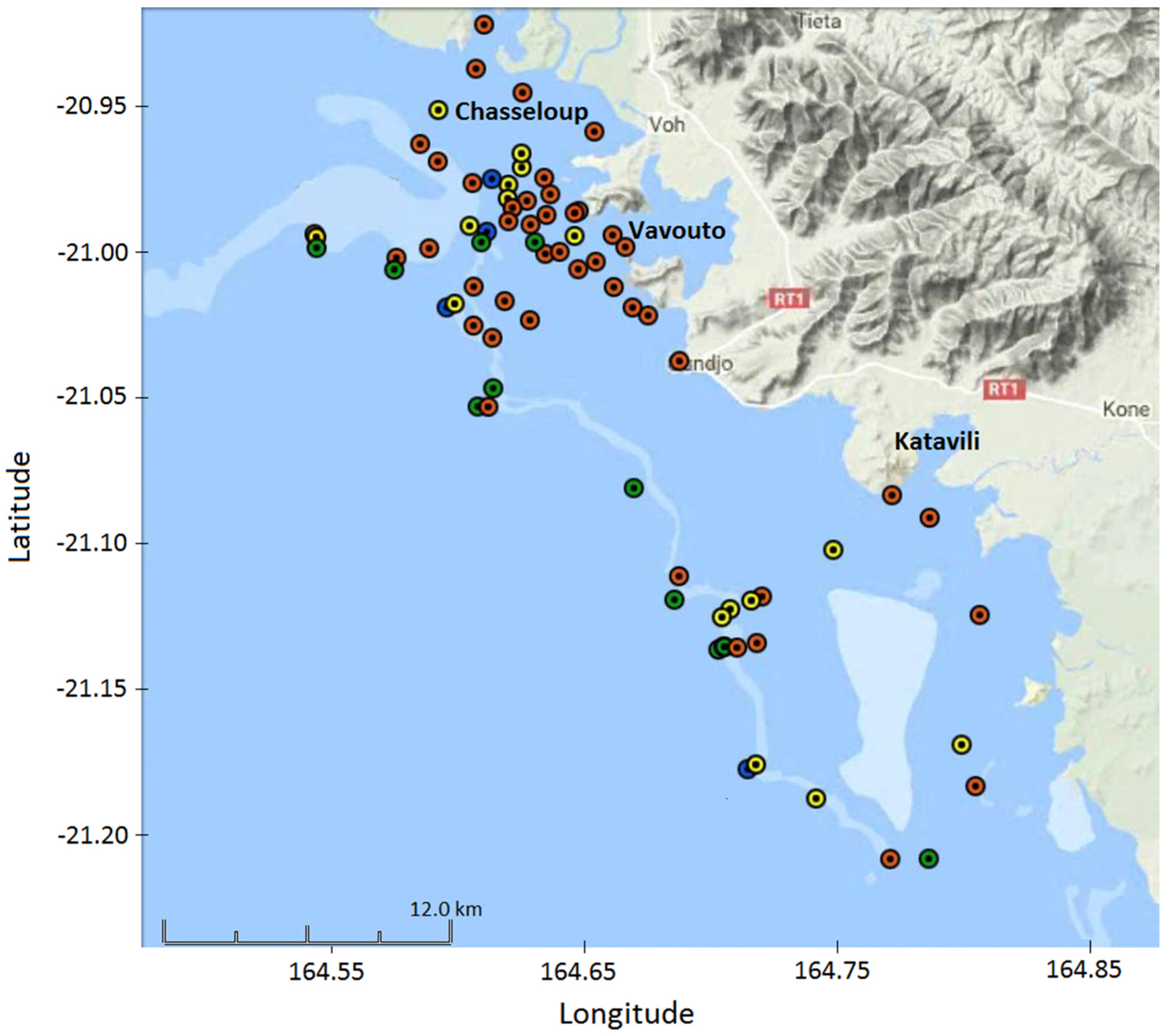
2.1. Study Area
2.2. Data
2.2.1. Field Measurements
2.2.2. Satellite Data
2.2.3. Match-Ups
2.3. Creation of the Support Vector Regression (SVR) Model
2.3.1. Sampling
2.3.2. Indicators
2.3.3. Support Vector Regression
2.3.4. Algorithm Steps
2.4. Interpolated Maps for In-situ Values
3. Results
3.1. Evaluation of the SVR Model at Visible Wavelengths
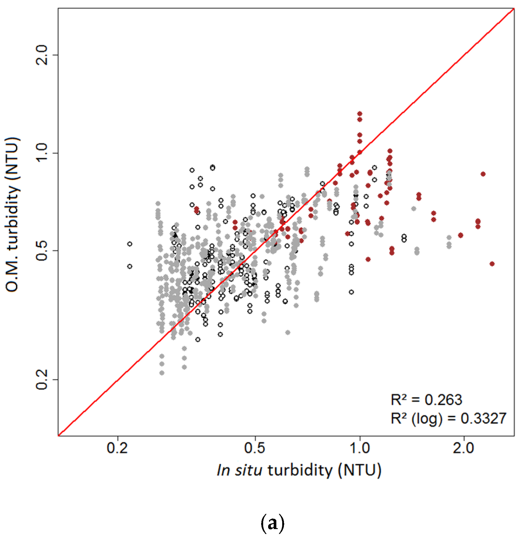
3.2. Comparison with Other Models
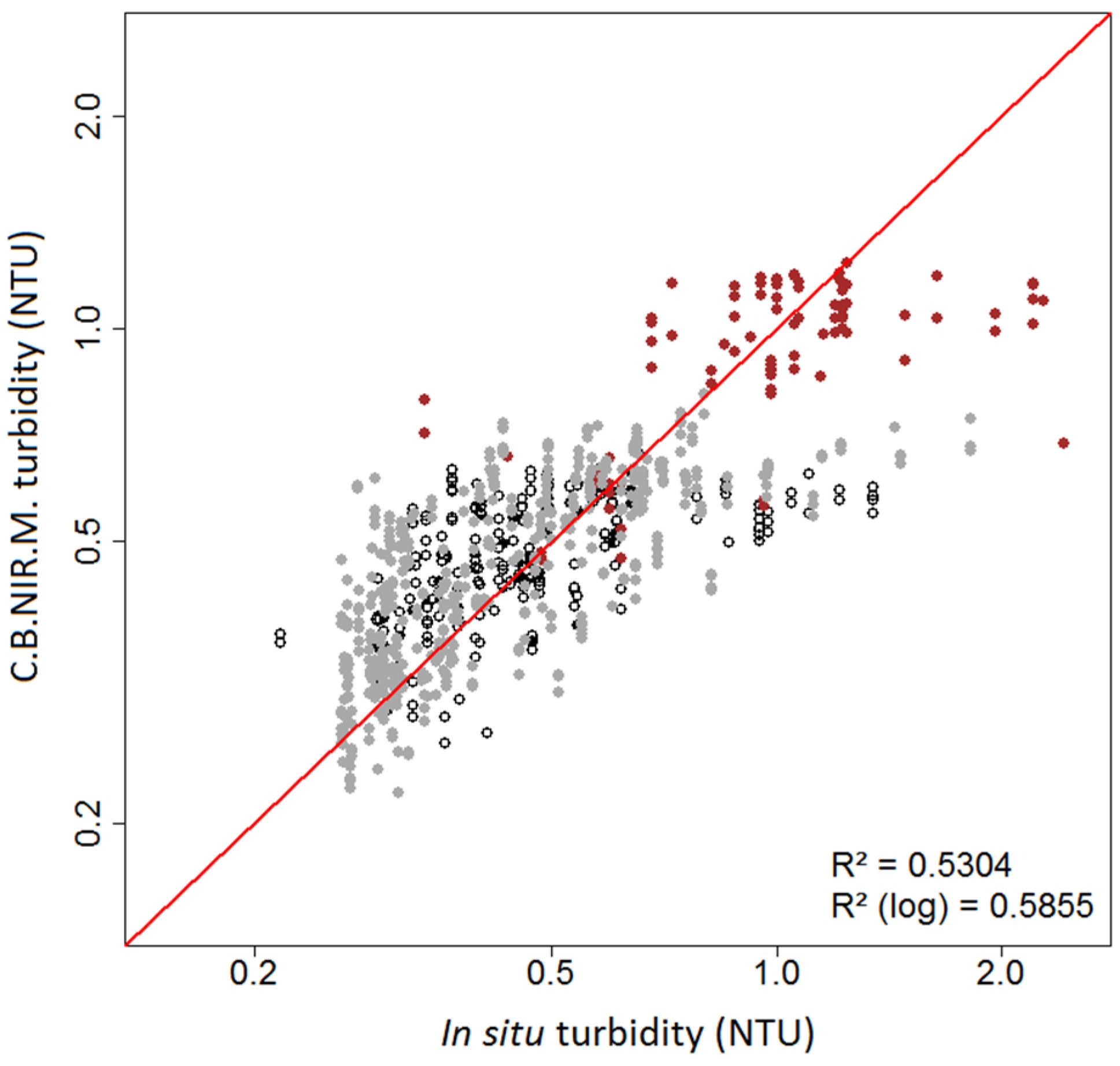
3.3. Using NIR Channels as Explanatory Variables
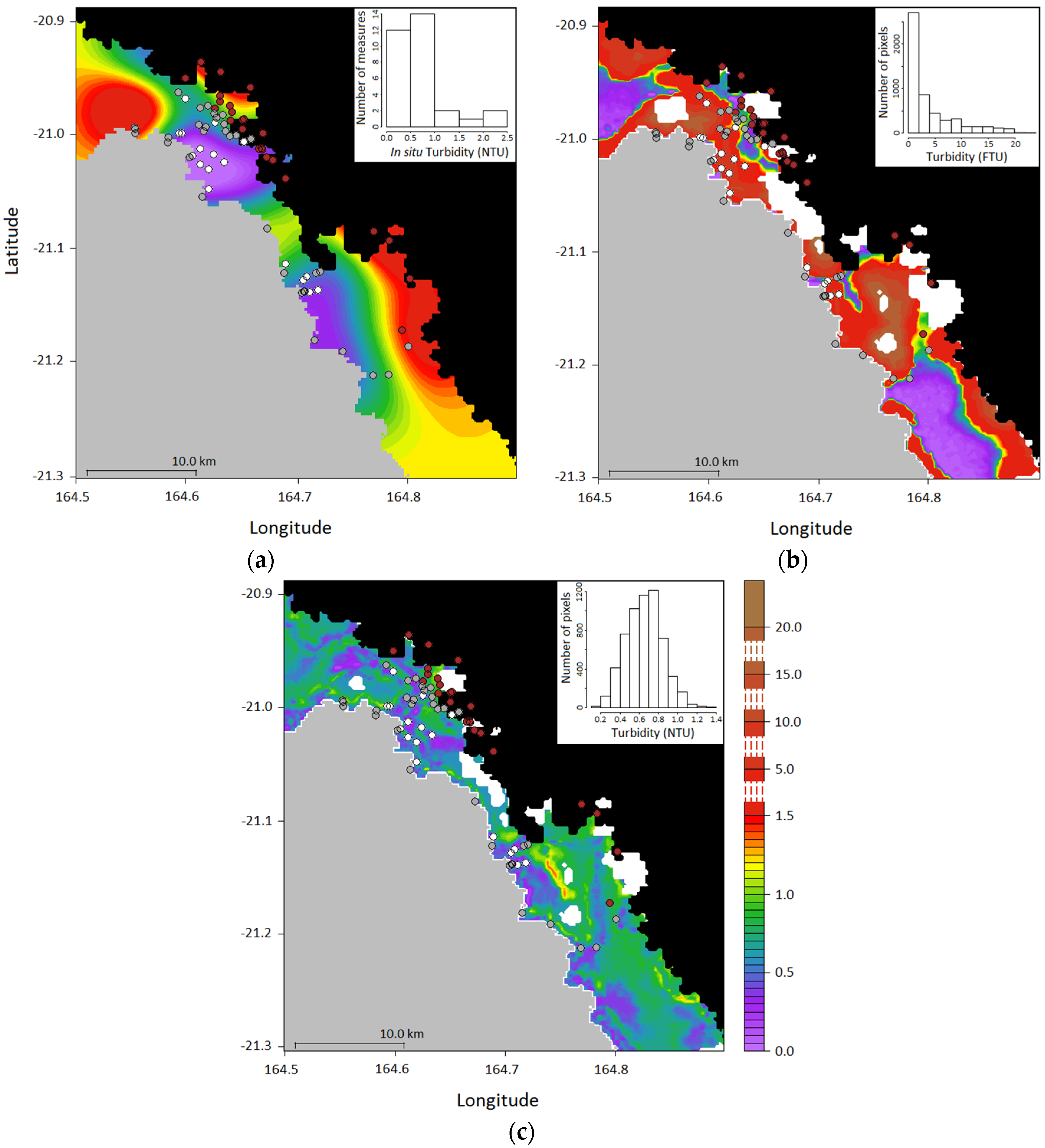
3.4. Application to MODIS Images
4. Discussion
4.1. Validity of the SVR for Turbidity or SPM Estimation, and Comparison to Previous Algorithms
4.2. Other Possible Improvements of Our Modelling Approach
4.2.1. Vertical Heterogeneity of In-situ Turbidity Profiles
4.2.2. Turbidity Values Distribution
4.2.3. Match-Up Research Procedure
4.2.4. Model Conception
4.2.5. Spectral Classification of MODIS Pixels in the VKP Lagoon
4.2.6. Including the Bottom Colour
5. Conclusions
Acknowledgments
Author Contributions
Conflicts of Interest
References
- Morrison, R.J.; Denton, G.; Tamata, U.B.; Grignon, J. Anthropogenic biogeochemical impacts on coral reefs in the Pacific Islands—An overview. Deep Sea Res. II 2013, 96, 5–12. [Google Scholar] [CrossRef]
- Fabricius, K.E.; Logan, M.; Weeks, S.; Brodie, J. The effects of river run-off on water clarity across the central Great Barrier Reef. Mar. Pollut. Bull. 2014, 84, 191–200. [Google Scholar] [CrossRef] [PubMed]
- Heinz, T.; Haapkylä, J.; Gilbert, A. Coral health on reefs near mining sites in New Caledonia. Dis. Aquat. Org. 2015, 115, 165–173. [Google Scholar] [CrossRef] [PubMed]
- Chen, Z.; Muller-Karger, F.; Hu, C. Remote sensing of water clarity in Tampa Bay. Remote Sens. Environ. 2007, 109, 249–259. [Google Scholar] [CrossRef]
- Adjeroud, M.; Fernandez, J.-M.; Carroll, A.G.; Harrison, P.L.; Penin, L. Spatial patterns and recruitment process of coral assemblages among contrasting environmental conditions in the southwestern lagoon of New Caledonia. Mar. Pollut. Bull. 2010, 61, 375–386. [Google Scholar] [CrossRef] [PubMed]
- Myers, N.; Mittermeier, R.A.; Mittermeier, C.G.; da Fonseca, G.A.B.; Kent, J. Biodiversity hotspots for conservation priorities. Nature 2000, 403, 853–858. [Google Scholar] [CrossRef] [PubMed]
- Alongi, D.M. Present state and future of the world’s mangrove forests. Environ. Conserv. 2002, 29, 331–349. [Google Scholar] [CrossRef]
- Adjeroud, M.; Gilbert, A.; Facon, M.; Foglia, M.; Moreton, B.; Heintz, T. Localised and limited impact of a dredging operation on coral cover in the northwestern lagoon of New Caledonia. Mar. Pollut. Bull. 2016, 105, 208–214. [Google Scholar] [CrossRef] [PubMed]
- Ceccarelli, D.M.; McKinnon, A.D.; Andréfouët, S.; Allain, V.; Young, J.; Gledhill, D.C.; Flynn, A.; Bax, N.J.; Beaman, R.; Borsa, P.; et al. The coral sea: Physical environment, ecosystem status and biodiversity assets. Adv. Mar. Biol. 2013, 66, 213–290. [Google Scholar] [PubMed]
- Cluzel, D.; Aitchison, J.C.; Picard, C. Tectonic accretion and underplating of mafic terranes in the Late Eocene intraoceanic fore-arc of New Caledonia (Southwest Pacific): Geodynamic implications. Tectonophysics 2001, 340, 23–59. [Google Scholar] [CrossRef] [Green Version]
- Perrier, N.; Ambrosi, J.P.; Colin, F.; Gilkes, R.J. Biogeochemistry of a Regolith: The New Caledonian Koniambo Ultramafic Massif. J. Geochem. Explor. 2006, 88, 54–58. [Google Scholar] [CrossRef]
- Fandeur, D.; Juillot, F.; Morin, G.; Olivi, L.; Cognigni, A.; Webb, S.M.; Brown, G.E. XANES evidence for oxidation of Cr(III)) to Cr(VI) by Mn-oxides in a lateritic regolith developed on serpentinized ultramafic rocks of New Caledonia. Environ. Sci. Technol. 2009, 43, 7384–7390. [Google Scholar] [CrossRef] [PubMed]
- Dublet, G.; Juillot, F.; Morin, G.; Fritsch, E.; Fandeur, D.; Ona-Nguema, G.; Brown, G.E. Ni speciation in a New Caledonian lateritic regolith: A quantitative X-ray absorption spectroscopy investigation. Geochim. Cosmochim. Acta 2012, 95, 119–133. [Google Scholar] [CrossRef]
- Dublet, G.; Juillot, F.; Morin, G.; Fritsch, E.; Fandeur, D.; Brown, G.E., Jr. Goethite aging explains Ni depletion in upper units of ultramafic lateritic ores from New Caledonia. Geochim. Cosmochim. Acta 2015, 160, 1–15. [Google Scholar] [CrossRef]
- Lagadec, G.; Perret, C.; Pitoiset, A. Nickel et Développement en Nouvelle-Calédonie, Perspectives de Développement Pour la Nouvelle-Calédonie; Perret, C., Ed.; PUG: Grenoble, France, 2002; Chapter 1; pp. 21–42. [Google Scholar]
- Join, J.L.; Robineau, B.; Ambrosi, J.P.; Costis, C.; Colin, F. Système hydrogéologique d’un massif minier ultrabasique de Nouvelle-Calédonie. C. R. Geosci. 2005, 337, 1500–1508. [Google Scholar] [CrossRef]
- Fernandez, J.-M.; Ouillon, S.; Chevillon, C.; Douillet, P.; Fichez, R.; Le Gendre, R. A combined modelling and geochemical study of the fate of terrigenous inputs from mixed natural and mining sources in a coral reef lagoon (New Caledonia). Mar. Poll. Bull. 2006, 52, 320–331. [Google Scholar] [CrossRef] [PubMed]
- Ouillon, S.; Douillet, P.; Lefebvre, J.P.; Le Gendre, R.; Jouon, A.; Bonneton, P.; Fernandez, J.M.; Chevillon, C.; Magand, O.; Lefèvre, J.; et al. Circulation and suspended sediment transport in a coral reef lagoon: The South-West lagoon of New Caledonia. Mar. Pollut. Bull. 2010, 61, 269–296. [Google Scholar] [CrossRef] [PubMed]
- Fernandez, J.M.; Meunier, J.D.; Ouillon, S.; Moreton, B.; Douillet, P.; Grauby, O. Dynamics of Suspended Sediments during a Dry Season and Their Consequences on Metal Transportation in a Coral Reef Lagoon Impacted by Mining Activities, New Caledonia. Water 2017, 9, 338. [Google Scholar] [CrossRef]
- Andrefouët, S.; Mumby, P.J.; McField, M.; Hu, C.; Muller-Karger, F.E. Revisiting coral reef connectivity. Coral Reefs 2002, 21, 43–48. [Google Scholar] [CrossRef]
- Dupouy, C.; Minghelli-Roman, A.; Despinoy, M.; Röttgers, R.; Neveux, J.; Pinazo, C.; Petit, M. MODIS/Aqua chlorophyll monitoring of the New Caledonia lagoon during the 2008 La Nina event. In Proceedings of the Remote Sensing of Inland, Coastal, and Oceanic Waters, Noumea, New Caledonia, 19 December 2008; Frouin, R.J., Andrefouët, S., Kawamura, H., Lynch, M.J., Pan, T., Platt, T., Eds.; SPIE: Bellingham, WA, USA, 2008; Volume 7150, pp. 1–8. [Google Scholar]
- Dupouy, C.; Röttgers, R.; Tedetti, M.; Martias, C.; Murakami, H.; Doxaran, D.; Lantoine, F.; Rodier, M.; Favareto, L.; Kampel, M.; et al. Influence of CDOM and Particle Composition on Ocean Colour of the Eastern New Caledonia Lagoon during the CALIOPE Cruises. Proc. SPIE 2014, 9261, 92610M. [Google Scholar] [CrossRef]
- Wang, Y.J.; Yan, F.; Zhang, P.Q.; Dong, W.J. Experimental research on quantitative inversion model of suspended sediment concentration using remote sensing technology. Chin. Geogr. Sci. 2007, 17, 243–249. [Google Scholar] [CrossRef]
- Gohin, F. Annual cycles of chlorophyll-a, non-algal suspended particulate matter, and Turbidity observed from space and in-situ in coastal waters. Ocean Sci. 2011, 7, 705–732. [Google Scholar] [CrossRef]
- Petus, C.; Chust, G.; Gohin, F.; Doxaran, D.; Froidefond, J.M.; Sagarminaga, Y. Estimating turbidity and total suspended matter in the Adour River plume (South Bay of Biscay) using MODIS 250-m imagery. Cont. Shelf Res. 2010, 30, 379–392. [Google Scholar] [CrossRef]
- Petus, C.; da Silva, E.T.; Devlin, M.; Wenger, A.S.; Álvarez-Romero, J.G. Using MODIS data for mapping of water types within river plumes in the Great Barrier Reef, Australia: Towards the production of river plume risk maps for reef and seagrass ecosystems. J. Environ. Manag. 2014, 137, 163–177. [Google Scholar] [CrossRef] [PubMed]
- Han, B.; Loisel, H.; Vantrepotte, V.; Mériaux, X.; Bryère, P.; Ouillon, S.; Dessailly, D.; Xing, Q.; Zhu, J. Development of a semi-analytical algorithm for the retrieval of Suspended Particulate Matter from remote sensing over clear to very turbid waters. Remote Sens. 2016, 8, 211. [Google Scholar] [CrossRef]
- Kabiri, K.; Moradi, M. Landsat-8 imagery to estimate clarity in near-shore coastal waters: Feasibility study—Chabahar Bay, Iran. Cont. Shelf Res. 2016, 125, 44–53. [Google Scholar] [CrossRef]
- Constantin, S.; Doxaran, D.; Constantinescu, S. Estimation of water turbidity and analysis of its spatio-temporal variability in the Danube River plume (Black Sea) using MODIS satellite data. Cont. Shelf Res. 2016, 112, 14–30. [Google Scholar] [CrossRef]
- Hu, C.; Chen, Z.; Clayton, T.D.; Swarzenski, P.; Brock, J.C.; Muller-Karger, F.E. Assessment of estuarine water-quality indicators using MODIS medium-resolution bands: Initial results from Tampa Bay, FL. Remote Sens. Environ. 2004, 93, 423–441. [Google Scholar] [CrossRef]
- Nechad, B.; Ruddick, K.G.; Park, Y. Calibration and validation of a generic multisensor algorithm for mapping of total suspended matter in turbid waters. Remote Sens. Environ. 2010, 114, 854–866. [Google Scholar] [CrossRef]
- Novoa, S.; Doxaran, D.; Ody, A.; Vanhellemont, Q.; Lafon, V.; Lubac, B.; Gernez, P. Atmospheric Corrections and Multi-Conditional Algorithm for Multi-Sensor Remote Sensing of Suspended Particulate Matter in Low-to-High Turbidity Levels Coastal Waters. Remote Sens. 2017, 9, 61. [Google Scholar] [CrossRef]
- Dogliotti, A.I.; Ruddick, K.G.; Nechad, B.; Doxaran, D.; Knaeps, E.A. single algorithm to retrieve turbidity from remotely-sensed data in all coastal and estuarine waters. Remote Sens. Environ. 2015, 156, 157–168. [Google Scholar] [CrossRef]
- Álvarez-Romero, J.G.; Devlin, M.J.; Teixeira da Silva, E.; Petus, C.; Ban, N.; Pressey, R.J.; Kool, J.; Roberts, S.; Cerdeira, W.A.; Brodie, J. A novel approach to model exposure of coastal-marine ecosystems to riverine flood plumes based on remote sensing techniques. J. Environ. Manag. 2013, 119, 194–207. [Google Scholar] [CrossRef] [PubMed]
- Devlin, M.; McKinna, L.W.; Álvarez-Romero, J.G.; Petus, C.; Abott, B.; Harkness, P.; Brodie, J. Mapping the pollutants in surface riverine flood plume waters in the Great Barrier Reef, Australia. Mar. Pollut. Bull. 2012, 65, 224–235. [Google Scholar] [CrossRef] [PubMed]
- Miller, R.L.; McKee, B.A. Using MODIS Terra 250 m imagery to map concentrations of total suspended matter in coastal waters. Remote Sens. Environ. 2004, 93, 259–266. [Google Scholar] [CrossRef]
- Doxaran, D.; Froidefond, J.M.; Castaing, P.; Babin, M. Dynamics of the turbidity maximum zone in a macrotidal estuary (the Gironde, France): Observations from field and MODIS satellite data. Estuar. Coast. Shelf Sci. 2009, 81, 321–332. [Google Scholar] [CrossRef]
- Lahet, F.; Stramski, D. MODIS imagery of turbid plumes in San Diego coastal waters during rainstorm events. Remote Sens. Environ. 2010, 114, 332–344. [Google Scholar] [CrossRef]
- Ouillon, S.; Douillet, P.; Petrenko, A.; Neveux, J.; Dupouy, C.; Froidefond, J.-M.; Andréfouët, S.; Muñoz-Caravaca, A. Optical Algorithms at satellite wavelengths for Total Suspended Matter in Tropical Coastal Waters. Sensors 2008, 8, 4165–4185. [Google Scholar] [CrossRef] [PubMed]
- Dupouy, C.; Neveux, J.; Ouillon, S.; Frouin, R.; Murakami, H.; Hochard, S.; Dirberg, G. Inherent optical properties and satellite retrieval of chlorophyll concentration in the lagoon and open waters of New Caledonia. Mar. Pollut. Bull. 2010, 61, 503–518. [Google Scholar] [CrossRef] [PubMed]
- Hochberg, E.J.; Atkinson, M. Capabilities of remote sensors to classify coral, algae, and sand as pure and mixed spectra. Remote Sens. Environ. 2003, 85, 174–189. [Google Scholar] [CrossRef]
- Minghelli-Roman, A.; Dupouy, C. Influence of water column chlorophyll concentration on bathymetric estimations in the lagoon of New Caledonia using several MERIS images. IEEE J. Sel. Top. Appl. Earth Obs. Remote Sens. 2013, 77, 1–7. [Google Scholar] [CrossRef] [Green Version]
- Minghelli-Roman, A.; Dupouy, C. Correction of the water column attenuation: Application to the seabed mapping of the lagoon of New Caledonia using MERIS images. IEEE J. Sel. Top. Appl. Earth Obs. Remote Sens. 2014, 7, 2617–2629. [Google Scholar] [CrossRef]
- Murakami, H.; Dupouy, C. Atmospheric correction and inherent optical property estimation in the southwest New Caledonia lagoon using AVNIR-2 high-resolution data. Appl. Opt. 2013, 52, 182–198. [Google Scholar] [CrossRef] [PubMed]
- McKinna, L.I.W.; Fearns, P.R.C.; Weeks, S.J.; Werdell, P.J.; Reichstetter, M.; Franz, B.A.; Shea, D.M.; Feldman, G.C. A semianalytical ocean colour inversion algorithm with explicit water column depth and substrate reflectance parameterization. J. Geophys. Res. Oceans 2015, 120, 1741–1770. [Google Scholar] [CrossRef]
- Reichstetter, M.; Fearns, P.R.C.S.; Weeks, S.J.; McKinna, L.I.W.; Roelfsema, C.; Furnas, M. Bottom reflectance in Ocean Colour Satellite Remote Sensing for Coral Reef Environments. Remote Sens. 2015, 7, 16756–16777. [Google Scholar] [CrossRef]
- Keiner, L.E.; Yan, X.H. A neural network model for estimating sea surface chlorophyll and sediments from Thematic Mapper imagery. Remote Sens. Environ. 1998, 66, 153–165. [Google Scholar] [CrossRef]
- Zhan, H. Application of Support Vector Machines in inverse problems in ocean colour remote sensing. Support Vector Mach. Theory Appl. 2005, 177, 387–398. [Google Scholar]
- Chen, J.; Quan, W.T.; Cui, T.W.; Song, Q.J. Estimation of total suspended matter concentration from MODIS data using a neural network model in the China eastern coastal zone. Est. Coast. Shelf Sci. 2015, 155, 104–113. [Google Scholar] [CrossRef]
- Zhan, H.; Shi, P.; Chen, C. Retrieval of oceanic chlorophyll concentration using support vector machines. IEEE Trans. Geosci. Remote Sens. 2003, 41, 2947–2951. [Google Scholar] [CrossRef]
- Drucker, H.; Burges, C.J.C.; Kaufman, L.; Smola, A.; Vapnik, V. Support Vector Regression Machines. Adv. Neural Inf. Process. Syst. 1996, 9, 155–161. [Google Scholar]
- Camps-Valls, G.; Bruzzone, L.; Rojo-Alvarez, J.L.; Melgeni, F. Robust Support Vector Regression for biophysical variable estimation from remotely sensed images. IEEE Geosci. Remote Sens. Lett. 2006, 3, 1–5. [Google Scholar] [CrossRef]
- Wattelez, G.; Dupouy, C.; Mangeas, M.; Lefèvre, J.; Touraïvane; Frouin, R. A statistical algorithm for estimating Chlorophyll Concentration in the New Caledonian lagoon. Remote Sens. 2016, 8, 45. [Google Scholar] [CrossRef] [Green Version]
- Touraïvane; Allenbach, M.; Mangeas, M.; Bonte, C. Monitoring the turbidity associated with the dredging in Vavouto Bay in New Caledonia. In Proceedings of the 19th International Congress on Modelling and Simulation, Perth, Australia, 12–16 December 2011. [Google Scholar]
- Leopold, A.; Marchand, C.; Renchon, A.; Deborde, J.; Quiniou, T.; Allenbach, M. Net ecosystem CO2 in the “Coeur de Voh” mangrove, New Caledonia: Effects of water stress on mangrove productivity in a semi-arid climate. Agric. For. Meteorol. 2016, 223, 217–232. [Google Scholar] [CrossRef]
- Banque des Données Bathymétriques de la Nouvelle-Calédonie (BDBNC). Banque des Données Bathymétriques de la Nouvelle-Calédonie; Atlas de la Direction des Technologies et Systèmes d’Information, Direction des Technologies et des Service de I’Information (DTSI): Noumea, France, 2009. [Google Scholar]
- Kumar-Roiné, S.; Achard, R.; Kaplan, H.; Haddad, L.; Laurent, A.; Drouzy, M.; Hubert, M.; Pluchino, S.; Fernandez, J.M. Suivi Environnemental du Milieu Marin de la Zone VKP; Volet 4: Surveillance Physicochimique. Période: Septembre 2015 —Août 2016 et Novembre 2016. Rapport AEL 131121-KS-02; AEL/LEA: Noumea, France, 2017. [Google Scholar]
- Bailey, S.W.; Werdell, P.J. A multi-sensor approach for the on-orbit validation of ocean colour satellite data products. Remote Sens. Environ. 2006, 102, 12–23. [Google Scholar] [CrossRef]
- Lefèvre, J. The VALHYSAT Project: MODIS-DB Database: Description Guide of the Database; Valhysat Report 1. Noumea: IRD Internal Report; IRD: Noumea, New Caledonia, 2010. [Google Scholar]
- Dupouy, C.; Savranski, T.; Lefèvre, J.; Despinoy, M.; Mangeas, M.; Fuchs, R.; Faure, V.; Ouillon, S.; Petit, M. Monitoring optical properties of the Southwest Tropical Pacific. In Proceedings of the Remote Sensing of the Coastal Ocean, Land, and Atmosphere Environment, Incheon, Korea, 4 November 2010; Frouin, R.J., Rhyong Yoo, H., Won, J.-S., Feng, A., Eds.; SPIE: Bellingham, WA, USA, 2010; Volume7858, p. 13. [Google Scholar] [CrossRef]
- R Core Team. R: A Language and Environment for Statistical Computing; R Foundation for Statistical Computing: Vienna, Austria, 2014. [Google Scholar]
- Jouon, A.; Ouillon, S.; Douillet, P.; Lefebvre, J.P.; Fernandez, J.-M.; Mari, X.; Froidefond, J.M. Spatio-temporal variability in suspended particulate matter concentration and the role of aggregation on size distribution in a coral reef lagoon. Mar. Geol. 2008, 256, 36–48. [Google Scholar] [CrossRef]
- Kaplan, H.; Laurent, A.; Hubert, M.; Moreton, B.; Kumar-Roiné, S.; Fernandez, J.M. Suivi de la Qualité Physico-Chimique de l’eau de mer de la Zone sud du Lagon de Nouvelle-Calédonie: 2ème Memester 2016; Contrat AEL/Vale-NC n°3052-Avenant n°1; AEL/LEA: Noumea, France, 2016. [Google Scholar]
- Jafar-Sidik, M.B.J.; Gohin, F.; Bowers, D.G.; Howarth, J.; Hull, T. The relationship between Suspended Particulate Matter and Turbidity at a mooring station in a coastal environment: Consequences for satellite-derived products. Oceanologia 2017, in press. [Google Scholar] [CrossRef]
- Shen, F.; Verhoef, W.; Zhou, Y.X.; Salama, M.S.; Liu, X.L. Satellite estimates of wide-range suspended sediment concentrations in Changjiang (Yangtze) estuary using MERIS data. Estuaries Coasts 2010, 33, 1420–1429. [Google Scholar] [CrossRef]
- Gordon, H.R.; Clarke, D.K. Remote sensing optical properties of a stratified ocean: An improved interpretation. Appl. Opt. 1980, 19, 3428–3430. [Google Scholar] [CrossRef] [PubMed]
- Nanu, L.; Robertson, C. The effect of suspended sediment depth distribution on coastal water spectral reflectance: Theoretical simulation. Int. J. Remote Sens. 1993, 14, 225–239. [Google Scholar] [CrossRef]
- Ouillon, S. An inversion method for reflectance in stratified turbid waters. Int. J. Remote Sens. 2003, 24, 535–548. [Google Scholar] [CrossRef]
- Fichez, R.; Chifflet, S.; Douillet, P.; Gérard, P.; Gutierrez, F.; Jouon, A.; Ouillon, S.; Grenz, C. Biogeochemical typology and temporal variability of lagoon waters in a coral reef ecosystem subject to terrigeneous and anthropogenic inputs (New Caledonia). Mar. Poll. Bull. 2010, 61, 309–322. [Google Scholar] [CrossRef] [PubMed]
- Lyzenga, D. Passive remote sensing techniques for mapping water depth and bottom features. Appl. Opt. 1978, 17, 379–383. [Google Scholar] [CrossRef] [PubMed]
- Tolk, B.L.; Han, L.; Rundquist, D.C. The impact of bottom brightness on spectral reflectance of suspended sediments. Int. J. Remote Sens. 2000, 21, 2259–2268. [Google Scholar] [CrossRef]
- Mobley, C.D.; Sundman, L.K. Effects of optically shallow bottoms on upwelling radiances: Inhomogeneous and slopping bottoms. Limnol. Oceanogr. 2003, 48, 329–336. [Google Scholar] [CrossRef]
- Lyzenga, D. Remote sensing of bottom reflectance and Water attenuation parameters in shallow water using aircraft and Landsat data. Int. J. Remote Sens. 1981, 2, 71–82. [Google Scholar] [CrossRef]
- Lyzenga, D.; Malinas, N.; Tanis, F. Multispectral Bathymetry Using a Simple Physically Based Algorithm. IEEE Trans. Geosci. Remote Sens. 2006, 44, 2251–2259. [Google Scholar] [CrossRef]
 : 0–10 m depth;
  : 10–20 m depth;
  : 20–30 m depth;
  : > 30 m depth.
: 0–10 m depth; : 10–20 m depth; : 20–30 m depth; : > 30 m depth.
: > 30 m depth.
: 0–10 m depth; : 10–20 m depth; : 20–30 m depth; : > 30 m depth.
 : white bottom;
  : grey bottom;
  : brown bottom; black areas correspond to land and those near the barrier reef are emerged reefs. (b) Histogram of the measured bathymetry on the visited stations. (c) Histogram of the in-situ turbidity values measured along CTD profiles.
: white bottom; : grey bottom; : brown bottom; black areas correspond to land and those near the barrier reef are emerged reefs. (b) Histogram of the measured bathymetry on the visited stations. (c) Histogram of the in-situ turbidity values measured along CTD profiles.
: brown bottom; black areas correspond to land and those near the barrier reef are emerged reefs. (b) Histogram of the measured bathymetry on the visited stations. (c) Histogram of the in-situ turbidity values measured along CTD profiles.
: white bottom; : grey bottom; : brown bottom; black areas correspond to land and those near the barrier reef are emerged reefs. (b) Histogram of the measured bathymetry on the visited stations. (c) Histogram of the in-situ turbidity values measured along CTD profiles. : white bottom; : grey bottom; : brown bottom.
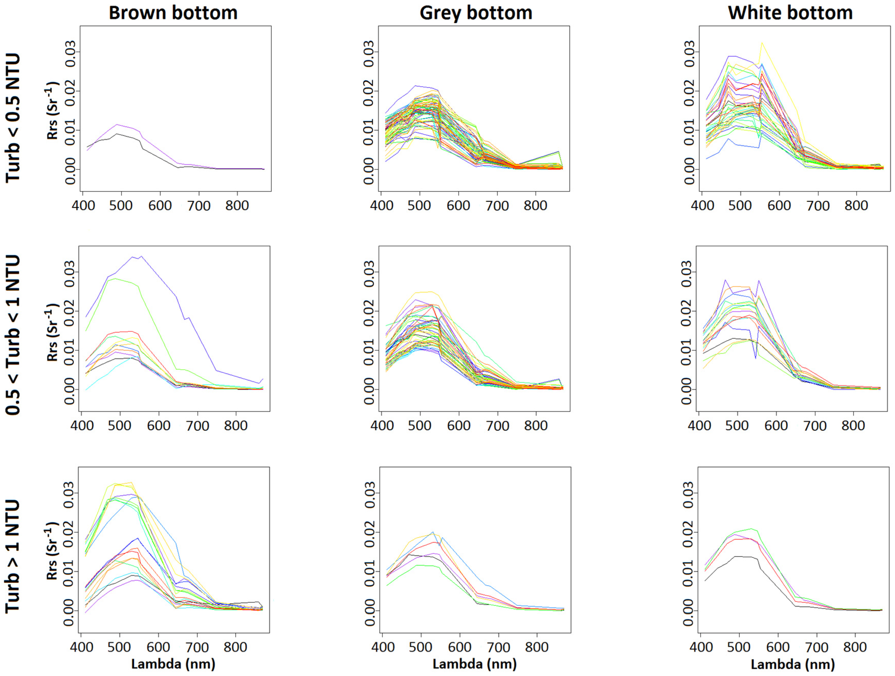
: white bottom; : grey bottom; : brown bottom.
: white bottom; : grey bottom; : brown bottom.

 : white bottom; : grey bottom; : brown bottom.
: white bottom; : grey bottom; : brown bottom.
: white bottom; : grey bottom; : brown bottom. : white bottom; : grey bottom; : brown bottom. On maps (b) and (c) the white areas correspond to flagged pixels.
: white bottom; : grey bottom; : brown bottom. On maps (b) and (c) the white areas correspond to flagged pixels.
: white bottom; : grey bottom; : brown bottom. On maps (b) and (c) the white areas correspond to flagged pixels. : white bottom; : grey bottom; : brown bottom. On maps (b) and (c) the white areas correspond to flagged pixels.
: white bottom; : grey bottom; : brown bottom. On maps (b) and (c) the white areas correspond to flagged pixels.
: white bottom; : grey bottom; : brown bottom. On maps (b) and (c) the white areas correspond to flagged pixels. : white bottom; : grey bottom; : brown bottom.
: white bottom; : grey bottom; : brown bottom.
: white bottom; : grey bottom; : brown bottom.


| Period | Number of CTD Stations | Number of Match-Ups | MODIS Files |
|---|---|---|---|
| 22–23/4/2014 | 31 | 30 | A2014111025500 |
| A2014113024000 | |||
| 19–29/5/2014 | 59 | 53 | A2014138023500 |
| A2014139032000 | |||
| A2014141030500 | |||
| A2014145024000 | |||
| A2014147023000 | |||
| 24–27/6/2014 | 43 | 40 | A2014173030500 |
| A2014175025500 | |||
| A2014177024000 | |||
| 28–30/7/2014 | 35 | 29 | A2014206021000 |
| A2014207025500 | |||
| A2014209024000 | |||
| A2014211023000 | |||
| A2014229021500 | |||
| 18–20/8/2014 | 8 | 7 | A2014227023000 |
| A2014229021500 | |||
| 28–30/10/2014 | 28 | 27 | A2014301030500 |
| A2014302021000 | |||
| 21–23/1/2015 | 34 | 34 | A2015021032500 |
| A2015024021500 | |||
| 19–27/3/2015 | 33 | 32 | A2015079022000 |
| A2015085032500 | |||
| A2015086023000 | |||
| 28–30/4/2015 | 24 | 19 | A2015116024000 |
| A2015117032500 | |||
| A2015121030000 | |||
| 6–7/5/2015 | 18 | 17 | A2015128030500 |
| 22–30/6/2015 | 36 | 35 | A2015173023500 |
| A2015174032000 | |||
| A2015175022500 | |||
| A2015176030500 | |||
| A2015180024000 | |||
| 22–27/7/2015 | 17 | 17 | A2015205023500 |
| A2015207022000 | |||
| 17–26/8/2015 | 35 | 26 | A2015228024000 |
| A2015234020500 | |||
| A2015236033000 | |||
| 28/9/2015–1/10/2015 | 47 | 45 | A2015272030500 |
| A2015273021000 | |||
| A2015274025000 | |||
| 26–30/10/2015 | 41 | 40 | A2015299024500 |
| A2015300033000 | |||
| A2015302031500 | |||
| 16–20/11/2015 | 39 | 39 | A2015325032500 |
| 22/12/2015 | 6 | 4 | A2015357032500 |
| C.B.O.M. | C.B.NIR.M. | ||||||||
|---|---|---|---|---|---|---|---|---|---|
| Indicators | Min. | Mean | Max. | p-Value | p-Value | Min. | Mean | Max. | p-Value |
| (t-Test 1) | (t-Test 2) | (t-Test 3) | |||||||
| MNB | −0.104 | −0.050 | 0.033 | 0.0371 # | 0.1659 * | −0.144 | −0.064 | −0.010 | 0.0439 * |
| MNAE | 0.211 | 0.233 | 0.262 | <0.001 * | <0.001 * | 0.219 | 0.234 | 0.269 | 0.5484 * |
| MAE | 0.094 | 0.139 | 0.172 | <0.001 * | <0.001 * | 0.109 | 0.136 | 0.174 | 0.1691 * |
| RMSE | 0.126 | 0.235 | 0.330 | <0.001 * | <0.001 * | 0.146 | 0.220 | 0.333 | 0.0156 * |
| R2 | 0.426 | 0.494 | 0.602 | <0.001 * | 0.0012 * | 0.402 | 0.553 | 0.633 | 0.0312 * |
| R2 (log) | 0.431 | 0.539 | 0.639 | <0.001 * | <0.001 * | 0.478 | 0.590 | 0.684 | 0.0141 * |
| In-situ values (NTU) | 0.216 | 0.549 | 2.417 | 0.216 | 0.549 | 2.417 | |||
| Assessment values (NTU) | 0.230 | 0.513 | 1.291 | 0.221 | 0.525 | 1.235 | |||
| Model | Min. | 1st Decile | 1st Quartile | Median | 3rd Quartile | 9th Decile | Max. |
|---|---|---|---|---|---|---|---|
| O2008 (FTU) | 0.0500 | 0.1360 | 0.4418 | 1.8898 | 5.6038 | 11.4643 | 23.4488 |
| B.O.M. (NTU) | 0.1036 | 0.4084 | 0.5195 | 0.6615 | 0.7768 | 0.8885 | 1.3938 |
| B.NIR.M. (NTU) | 0.2294 | 0.3880 | 0.4503 | 0.6029 | 0.7264 | 0.8191 | 1.3116 |
| Model | Min. | 1st Decile | 1st Quartile | Median | 3rd Quartile | 9th Decile | Max. |
|---|---|---|---|---|---|---|---|
| O2008 (FTU) | 0.0500 | 0.05 | 0.1209 | 0.7162 | 3.2655 | 6.8045 | 30.0500 |
| B.O.M. (NTU) | 0.1190 | 0.3935 | 0.4862 | 0.6373 | 0.7611 | 0.8964 | 1.4139 |
| B.NIR.M (NTU) | 0.2232 | 0.4104 | 0.5125 | 0.6465 | 0.7914 | 0.8904 | 1.3017 |
© 2017 by the authors. Licensee MDPI, Basel, Switzerland. This article is an open access article distributed under the terms and conditions of the Creative Commons Attribution (CC BY) license (http://creativecommons.org/licenses/by/4.0/).
Share and Cite
Wattelez, G.; Dupouy, C.; Lefèvre, J.; Ouillon, S.; Fernandez, J.-M.; Juillot, F. Application of the Support Vector Regression Method for Turbidity Assessment with MODIS on a Shallow Coral Reef Lagoon (Voh-Koné-Pouembout, New Caledonia). Water 2017, 9, 737. https://doi.org/10.3390/w9100737
Wattelez G, Dupouy C, Lefèvre J, Ouillon S, Fernandez J-M, Juillot F. Application of the Support Vector Regression Method for Turbidity Assessment with MODIS on a Shallow Coral Reef Lagoon (Voh-Koné-Pouembout, New Caledonia). Water. 2017; 9(10):737. https://doi.org/10.3390/w9100737
Chicago/Turabian StyleWattelez, Guillaume, Cécile Dupouy, Jérôme Lefèvre, Sylvain Ouillon, Jean-Michel Fernandez, and Farid Juillot. 2017. "Application of the Support Vector Regression Method for Turbidity Assessment with MODIS on a Shallow Coral Reef Lagoon (Voh-Koné-Pouembout, New Caledonia)" Water 9, no. 10: 737. https://doi.org/10.3390/w9100737