An Analytical Model of Fickian and Non-Fickian Dispersion in Evolving-Scale Log-Conductivity Distributions

Abstract

The characteristics of solute transport within log-conductivity fields represented by power-law semi-variograms are investigated by an analytical Lagrangian approach that accounts for the automatic frequency cut-off induced by the initial contaminant plume size. The transport process anomaly is critically controlled by the magnitude of the Péclet number. Interestingly enough, unlike the case of fast-decaying correlation functions (i.e., exponential or Gaussian), the presence of intensive transverse diffusion acts as an antagonist mechanism in the process of Fickian regime achievement. On the other hand, for markedly advective conditions and finite initial plume size, even the ergodic longitudinal dispersion coefficient turns out to be asymptotically constant, and the corresponding expected concentration distribution can therefore be obtained by conventional mathematical methods.

1. Introduction

Modeling the considerable spatial variability exhibited by the hydraulic properties of natural porous formations such as oil reservoirs and aquifers is a key requirement for the monitoring and control of the related flow and transport processes. The classic stochastic theories (e.g., [1,2]) assume that the log-conductivity Y(x) = ln K(x), where K is the local hydraulic conductivity and x is the vector of spatial coordinates, is a homogeneous random space function, normally distributed and completely characterized by constant mean and variance and by a fast-decaying correlation function. The above characteristics imply the existence of a single representative scale of heterogeneity, i.e., the so-called integral scale.

However, in the case of regional transport processes (i.e., over horizontal distances of the order of tens to hundreds aquifer thicknesses), due to the involvement of several geological units called facies, solute transport is typically influenced by several scales of structural variability. According to Neuman [3], the log-K distribution resulting from the coexistence of geological facies might be represented by a complex hierarchy of scales, progressively coming into play as the travel distance increases. In this case, the semi-variogram of Y (i.e., the variance of log-K spatial increments) tends to increase with no asymptotic threshold and likely in a discontinuous fashion. To describe such media in a mathematical framework, the authors of [3] adopted the simple-scaling model, represented by a power-law semi-variogram, γ_Y(r) = ar^b, where a is a dimensional constant and one-half of the scaling exponent H = b/2 is known as the Hurst coefficient [4].

The presence of significant log-conductivity trends affects flow and transport in aquifers to an extent that depends on the complexity of the geologic formation. Additionally, at the regional scale, the more appropriate models of flow and transport are two-dimensional. In this case, the hydraulic properties of the heterogeneous formation, suitably described by the log-transmissivity Y(x) = ln T(x), where the transmissivity T indicates the vertical average of K, are critically influenced by the depositional process. In such context, although the existence of several scales of heterogeneity seems reasonable, there is no direct experimental evidence supporting the power-law model. Neuman [3] provided an indirect justification of it, analyzing the scaling behavior exhibited by the longitudinal dispersivity of tracer plumes.

The spreading of solutes is usually investigated in terms of a longitudinal dispersion coefficient. There are two different types of dispersion coefficient. The ergodic dispersion coefficient is given by the time-rate of change of the single-particle position covariance and incorporates the uncertainty related to the plume centroid location; the effective dispersion coefficient consists in the time-rate of change of the expected longitudinal central spatial moment and only accounts for the heterogeneity at the plume scale. The difference between them was discussed by Fischer et al. [5] in the context of turbulent mixing; by Kitanidis [6], Dagan [7], and Rajaram and Gelhar [8] in the context of transport in natural single-scale porous formations; and by Glimm et al. [9] in the context of transport in natural evolving-scale porous formations. The investigation of longitudinal dispersion in a stochastic framework was later extended by Pannone to river-flow solute transport in the presence of random morphological heterogeneities based on a first-order formulation [10,11], and to strictly uniform river-flows by an exact closed-form solution based on the Taylor-Aris method of moments [12].

The implications of the ergodic or non-ergodic assumption for transport in evolving-scale formations were further discussed by Dagan [13]. In this study, among other things, the author obtained first-order analytical solutions for the effective dispersion coefficient in formations described by power-law semi-variograms. The main finding of the paper was that the ergodic assumption, implicit in most theoretical results of stochastic models, cannot be assumed as generally valid. As a consequence, rather than showing an anomalous continuous growth, effective dispersion in evolving-scale formations reaches a Fickian asymptotic limit for b < 1. The transport anomaly was only recovered for b > 1, but, in this case, the hypothesis of stationarity (on which the analytical treatment of transport was based) becomes strongly questionable.

The analytical solutions provided by Bellin et al. [14] substantially confirmed Dagan’s conclusions concerning the occurrence of anomalous dispersion for b > 1 and asymptotically Fickian dispersion for b < 1. Additionally, the assumption of linearity typical of any analytical approach was relaxed and tested by solving fully nonlinear flow and transport problems. For b < 1, the analytical and numerical solutions provided by [14] were in good agreement. Conversely, for large b (i.e., b = 1.75), the numerical solutions slightly overestimated the analytical ones. The anomalous dispersion predicted by the analytical solution was confirmed by the numerical results, at least in the explored range of variability of the log-conductivity variance (${\sigma }_Y^2<2$). Furthermore, the effective dispersion coefficient turned out to be not affected by the travel-distance cutoff, which was a consequence of the use of finite 2-D field dimensions in the numerical simulations.

Anomalous transport manifests itself in different forms, typically appearing as long tails in the spatial and/or temporal distributions of solute concentrations at given locations [15]. This tailing is classically interpreted as a result of peculiar solute spreading, associated with the existence of multiple scales of medium heterogeneity. Establishing a direct connection between continuous time random walk parameters and randomly heterogeneous hydraulic conductivity within uniform- mean flow domains, the authors of [15] showed that the features of transport cannot be explained by the structural disorder of the geologic formations only. On the contrary, dynamic/flow factors such as low-conductivity transition zones and preferential flow paths critically control the process. Based on that, it can easily be understood how the occurrence of non-Fickian behavior is a highly probable event in cases of transport through fractures [16,17].

Using first-order approximations in velocity fluctuations, the study by Suciu et al. [18] showed how anomalous super-diffusive behavior may result from the linear combination of independent random fields characterized by short-range correlation functions and increasing integral scales, e.g., [3,19]. According to the same type of linear decomposition of log-conductivity fluctuations, the present work proposes a new theoretical approach for the determination of an ergodic macro-dispersion coefficient depending on the initial plume size and the Péclet number magnitude, which is a measure of the relative importance of advective and diffusive-like transport mechanisms.

Detailed investigations of the relationship between injection modes and heterogeneity in the dispersion of solute particles in fracture networks able to store parts of solute mass were recently conducted by [20,21,22]. Based on the results in [20,21], the type of injection mode has a significant persistent impact on dispersion in a fracture network; more so for larger heterogeneity. The late arrivals for resident injection are several orders of magnitude larger than those related to flux injection, indicating that dispersion along the macroscopic flow direction is significantly enhanced by resident injection. Conversely, the study by [22] showed that, after accounting for a pre-asymptotic regime, the mean travel time of particles inserted using both resident and flux-weighted injection conditions scales linearly, and the tails of the corresponding breakthrough curves exhibit almost identical power laws. Demmy et al. [23] had previously studied the effect of injection modes in heterogeneous porous media. They had found that, for a general case of three-dimensional heterogeneity, uniform resident injection was associated with the nonlinear propagation of mean arrival time, whereas injection in flux was associated with linear propagation. Both injection modes yielded nonlinear arrival time variances, tending to some common asymptotic linear behavior. The moments of the flux-weighted curves were persistently lower than those characterizing the uniform resident injection case, although their propagation rates were converging toward some common value. Dentz et al. [24] developed a continuous time random walk approach for the evolution of Lagrangian velocities in steady heterogeneous flows based on a stochastic relaxation process for the streamwise particle velocities. They predicted Lagrangian particle dynamics starting from an arbitrary initial condition based on the Eulerian velocity distribution and a characteristic correlation scale. The main result of the study can be synthesized in the detection of strong Lagrangian correlation and anomalous dispersion for velocity distributions that are tailed toward low values, as well as in pronounced differences depending on the initial conditions. Note that all mentioned studies ([20,21,22,23,24]) investigate the relationship between injection modes and advective heterogeneity on solute dispersion without discussing the effect of local dispersion magnitude. This effect is expected to be definitely more pronounced for transport in porous media, which is the focus of the present study.

The crucial role of local dispersion (sometimes simply named ‘diffusion’) in solute macro-dispersion and dilution was already explored in the context of subsurface flow and transport by Pannone and Kitanidis [25] and in the context of river-flow and transport by Pannone [26,27]. Overall, these studies showed that, in the case of heterogeneous structures characterized by short-range correlations, macro-dispersion and dilution are singularly driven by the interplay of advective heterogeneities and diffusive-like mechanisms.

The results of the present investigation, which focuses on the interplay between evolving-scale heterogeneity and diffusion in longitudinal dispersion for uniform instantaneous injections of different sizes, and invariably predicts asymptotically Fickian macro-dispersion for purely advective regimes and super-diffusive transport in the presence of non-negligible local dispersion (regardless of scaling exponent value), are partly in contrast with what has previously been found by similar studies on this topic.

2. Formulation

Let us consider a first type of isotropic power-law semi-variogram, with an exponent ranging between 0 and 1:

$${\gamma }_Y\left(r\right)=a{r}^{b}0<b<1$$

(1)

It can be shown that such a semi-variogram is obtained by the superposition of an infinite hierarchy of independent stationary log-conductivity fields characterized by an exponential covariance function, an increasing integral scale, and variance proportional to it (see also [3]). The total fluctuation of the random function Y(x) = lnK(x) = < Y > + Y’(x), where the angle brackets indicate the (assumed constant) ensemble mean and the prime indicates the deviation about that mean, is given by:

$$Y^{\prime }\left(x\right)={\displaystyle \sum _{\mathrm{\Lambda }=0}^{\infty }{Y}_{\mathrm{\Lambda }}^{\prime }}\left(x\right)$$

(2)

where $Y_{\mathrm{\Lambda }}^{\prime }$ is the fluctuation associated with the Λ^th order of the hierarchy. The generic heterogeneous sub-unit is therefore represented by the superposition of a given finite number of stationary fields of increasing order:

$$Y^{\left(m\right)}\left(x\right)={\displaystyle \sum _{\mathrm{\Lambda }=m}^{\infty }{Y}_{\mathrm{\Lambda }}^{\prime }}\left(x\right)$$

(3)

For each stationary field, one has:

$${\gamma }_{Y\mathrm{\Lambda }}\left(r\right)={\sigma }_{Y\mathrm{\Lambda }}^2\left(I_{Y\mathrm{\Lambda }}\right)\left[1-\exp \left(-r/I_{Y\mathrm{\Lambda }}\right)\right]$$

(4)

where the integral scale $I_{Y\mathrm{\Lambda }}$ can be viewed as the inverse of the wave-number Λ, which represents the spatial periodicity of the associated log-conductivity heterogeneity:

$$I_{Y\mathrm{\Lambda }}=\frac{1}{\mathrm{\Lambda }}$$

(5)

Let us assume that the corresponding variance ${\sigma }_{Y\mathrm{\Lambda }}^2$ is a negative power of Λ:

$${\sigma }_{Y\mathrm{\Lambda }}^2=\frac{c}{{\mathrm{\Lambda }}^{1+\beta }}0<\beta <1$$

(6)

where c is a dimensional constant. Integrating over all the possible wave-numbers:

$${\gamma }_Y\left(r\right)={\displaystyle \underset{0}{\overset{\infty }{\int }}\frac{c}{{\mathrm{\Lambda }}^{1+\beta }}\left[1-\exp \left(-r\mathrm{\Lambda }\right)\right]}d\mathrm{\Lambda }$$

(7)

one obtains [28]:

$${\gamma }_Y\left(r\right)=-c\mathrm{\Gamma }\left(-\beta \right)r^{\beta }$$

(8)

where the symbol Γ indicates a Gamma function. Equation (8) coincides with Equation (1) if:

$$b=\beta a=-c\mathrm{\Gamma }\left(-b\right)$$

(9)

For semi-variogram exponents ranging between 1 and 2:

$${\gamma }_Y\left(r\right)=a{r}^{b}1\le b<2$$

(10)

it can be shown that the statistically independent components of the hierarchy must be characterized by a Gaussian log-conductivity covariance function (see also [18]):

$${\gamma }_{Y\mathrm{\Lambda }}\left(r\right)={\sigma }_{Y\mathrm{\Lambda }}^2\left(I_{Y\mathrm{\Lambda }}\right)\left[1-\exp \left(-r^2/l_{Y\mathrm{\Lambda }}^2\right)\right]$$

(11)

where $l_{Y\mathrm{\Lambda }}$ indicates the corresponding correlation length ($l_{Y\mathrm{\Lambda }}=2I_{Y\mathrm{\Lambda }}/\sqrt{\pi }$) and the variance is given by:

$${\sigma }_{Y\mathrm{\Lambda }}^2=\frac{c}{{\mathrm{\Lambda }}^{2+\beta }}0\le \beta <1$$

(12)

Integrating over Λ:

$${\gamma }_Y\left(r\right)={\displaystyle \underset{0}{\overset{\infty }{\int }}\frac{c}{{\mathrm{\Lambda }}^{2+\beta }}\left[1-\exp \left(-\pi r^2{\mathrm{\Lambda }}^2/4\right)\right]}d\mathrm{\Lambda }$$

(13)

one obtains [28]:

$${\gamma }_Y\left(r\right)=-c\mathrm{\Gamma }\left(-\frac{\beta +1}{2}\right){\left(\frac{\pi }{4}\right)}^{\frac{\beta +1}{2}}{r}^{\beta +1}$$

(14)

Equation (14) coincides with Equation (10) if:

$$b=\beta +1a=-c\mathrm{\Gamma }\left(-\frac{b}{2}\right){\left(\frac{\sqrt{\pi }}{2}\right)}^b$$

(15)

Given the mutual independence of the short-range log-conductivity fields, one can consider the whole hierarchy as decomposed into two different macroscopic components:

$$Y^{\prime }\left(x\right)=\tilde{Y}\left(x\right)+\overline{Y}\left(x\right)$$

(16)

where

$$\tilde{Y}\left(x\right)={\displaystyle \sum _{\mathrm{\Lambda }=N+1}^{\infty }{Y}_{\mathrm{\Lambda }}^{\prime }\left(x\right)}$$

(17)

identifies the log-conductivity fluctuation due to the (N+1)^th heterogeneous sub-unit and

$$\overline{Y}\left(x\right)={\displaystyle \sum _{\mathrm{\Lambda }=0}^N{Y}_{\mathrm{\Lambda }}^{\prime }\left(x\right)}$$

(18)

is the log-conductivity fluctuation induced by the larger scales of heterogeneity.

From Darcy’s law combined with the equation of continuity for incompressible fluids in incompressible solid matrices, one obtains the following steady flow equation:

$$\begin{array}{l}{\nabla }^{2}h\left(x\right)+\nabla h\left(x\right)\cdot \nabla Y\left(x\right)\\ ={\nabla }^2{h}^{\prime }\left(x\right)-J\cdot \nabla Y^{\prime }\left(x\right)+\nabla h^{\prime }\left(x\right)\cdot \nabla Y^{\prime }\left(x\right)=0\end{array}$$

(19)

where h indicates the hydraulic head and

$$J=-\nabla <h\left(x\right)>$$

(20)

indicates the mean head loss. In the Fourier domain, Equation (19) becomes:

$${\left|k\right|}^2\widehat{h}\left(k\right)+{\displaystyle \underset{k^{\prime }}{\int }{k}^{\prime }}\cdot \left(k-k^{\prime }\right)\widehat{Y}\left(k-k^{\prime }\right)\widehat{h}\left(k\prime \right)d{k}^{\prime }=\frac{j}{2\pi }J\cdot k\widehat{Y}\left(k\right)$$

(21)

where $j=\sqrt{-1}$ and the circumflex accent indicates Fourier transforms:

$$\widehat{h}\left(k\right)={\displaystyle \underset{x}{\int }{h}^{\prime }\left(x\right)}\exp \left(-j2\pi k\cdot x\right)dx$$

(22)

$$\widehat{Y}\left(k\right)={\displaystyle \underset{x}{\int }{Y}^{\prime }\left(x\right)}\exp \left(-j2\pi k\cdot x\right)dx$$

(23)

Let us assume that constant c is so small that, even for the larger sub-units, the log-conductivity variance is always finite and not larger than 1. Physically speaking, that means that the present theory concerns geologic formations made of nested (fractal-like), though mildly heterogeneous, porous structures. In this case, flow and transport linear theory (e.g., [1]) applies and the convolution term in Equation (21) can be neglected:

$${\left|k\right|}^2\widehat{h}\left(k\right)=\frac{j}{2\pi }J\cdot k\widehat{Y}\left(k\right)$$

(24)

Incidentally, as mentioned above, the 2-D numerical simulations by Bellin et al. [14] allowed it to be established that linear theory practically applies for log-transmissivity variance up to two. Similarly, from the first-order Darcy’s law (e.g., [1]):

$${\widehat{v}}_i\left(k\right)=\widehat{Y}\left(k\right)\left(U_i-{\displaystyle \sum _{j=1}^3\frac{k_i{k}_j}{{\left|k\right|}^2}{U}_j}\right)$$

(25)

where ${\widehat{v}}_i$ is the Fourier transform of the i^th component of velocity fluctuation and U = (U₁,U₂,U₃) is the constant ensemble mean velocity. From Equations (24) and (25) one can see that, at the first-order in the log-conductivity variance, each Fourier component of the log-conductivity field corresponds to a single component of hydraulic head and velocity. Therefore, the same properties of linear superposition holding for Y (see Equation (2)) apply to h and v as well. Consider now an initial solute injection at a uniform concentration C₀, confined within a volume

$$V_0=l_0^3$$

(26)

such that

$$I_{YN+1}<l_0<I_{YN}$$

(27)

The trajectory of the generic solute particle belonging to the dispersing plume can be expressed as:

$$\begin{array}{l}X\left(t,a\right)=a+{\displaystyle \underset{0}{\overset{t}{\int }}v\left[X\left(\tau ,a\right)\right]d\tau }+X_B\left(t\right)\\ =a+{\displaystyle \underset{0}{\overset{t}{\int }}\langle v\left[X\left(\tau ,a\right)\right]\rangle d\tau +{\displaystyle \underset{0}{\overset{t}{\int }}{v}^{\prime }\left[X\left(\tau ,a\right)\right]d\tau }}+X_B\left(t\right)\end{array}$$

(28)

where vector a represents its initial position within V₀, t is the time, and X_B the zero-mean Brownian component. Given Equations (16) and (25), it is also:

$$X\left(t,a\right)=a+Ut+X^{\prime }\left(t,a\right)+X_B\left(t\right)=a+Ut+\tilde{X}\left(t,a\right)+\overline{X}\left(t,a\right)+X_B\left(t\right)$$

(29)

where, at the first order:

$$\tilde{X}\left(t,a\right)={\displaystyle \sum _{\mathrm{\Lambda }=N+1}^{\infty }{X}_{\mathrm{\Lambda }}^{\prime }}\left(t,a\right)={\displaystyle \underset{0}{\overset{t}{\int }}\tilde{v}\left[X\left(\tau ,a\right)\right]d\tau }\cong {\displaystyle \underset{0}{\overset{t}{\int }}\tilde{v}\left[a+U\tau +X_B\left(\tau \right)\right]d\tau }$$

(30)

and

$$\overline{X}\left(t,a\right)={\displaystyle \sum _{\mathrm{\Lambda }=0}^N{X}_{\mathrm{\Lambda }}^{\prime }}\left(t,a\right)\cong {\displaystyle \underset{0}{\overset{t}{\int }}\overline{v}\left[a+U\tau +X_B\left(\tau \right)\right]d\tau }$$

(31)

Notice that, due to the linearization involved in Equations (30) and (31), the solute particles sample the velocity distribution along longitudinal deterministic trajectories (a + Uτ), disturbed only by the local-dispersive contribution represented by X_B. Such an assumption is common to all first-order (linearized) analytical formulations of subsurface flow and transport. Its physical meaning is that one neglects the self-feeding mechanism of advective dispersion that would emerge from the solution of the exact integro-differential equation:

$$X\prime \left(t,a\right)={\displaystyle \underset{0}{\overset{t}{\int }}{v}^{\prime }\left[a+U\tau +X^{\prime }\left(\tau ,a\right)+X_B\left(\tau \right)\right]d\tau }$$

(32)

A possible theoretical justification of it is that, overall, the reduced spreading of the particle sampling cloud left to the only Brownian component of fluctuation balances the more persistent correlation (and, therefore, the slower spreading) that would be induced by the advective fluctuation.

The concentration spatial moments, i.e., total mass, centroid and inertia, can respectively be calculated from:

$$M={\displaystyle \int nCdx}$$

(33)

$$R\left(t\right)=\frac{1}{M}{\displaystyle \int nCxdx}$$

(34)

and

$$S_{ij}\left(t\right)=\frac{1}{M}{\displaystyle \int nC\left(x_i-R_i\right)\left(x_j-R_j\right)dx}$$

(35)

where C = C(x,t) indicates the concentration in x at time t. For a single-particle injection in x = a (e.g., [1]):

$$\Delta C\left(x,t\right)=\frac{\Delta M}{n}\delta \left[x-X\left(t,a\right)\right]=\frac{C_0\left(a\right)n_{0}da}{n}\delta \left[x-X\left(t,a\right)\right]$$

(36)

where δ indicates Dirac’s distribution, ∆M is the associated mass, C₀ is the associated initial concentration, n is the generic volume porosity, and n₀ is the volume porosity at injection site. Integrating over the whole initial volume V₀ for n ≅ n₀ gives:

$$C\left(x,t\right)={\displaystyle \underset{V_0}{\int }{C}_0\left(a\right)}\delta \left[x-X\left(t,a\right)\right]da$$

(37)

The substitution of Equation (37) into Equations (34) and (35) for C₀ = const and M = n₀C₀V₀ yields:

$$R\left(t\right)=\frac{1}{V_0}{\displaystyle \underset{V_0}{\int }X\left(t,a\right)}da=\overline{a}+Ut+\frac{1}{V_0}{\displaystyle \underset{V_0}{\int }\left[X^{\prime }\left(t,a\right)+X_B\left(t\right)\right]}da$$

(38)

and

$$\begin{array}{l}{S}_{ij}\left(t\right)=\frac{1}{V_0}{\displaystyle \underset{V_0}{\int }\left[X_i\left(t,a\right)-R_i\left(t\right)\right]\left[X_j\left(t,a\right)-R_j\left(t\right)\right]da}\\ =S_{ij}\left(0\right)+\frac{1}{V_0}{\displaystyle \underset{V_0}{\int }\left[X_i^{\prime }\left(t,a\right)-\frac{1}{V_0}{\displaystyle \underset{V_0}{\int }{X}_i^{\prime }\left(t,a^{\prime }\right)d{a}^{\prime }}\right]}\left[X_j^{\prime }\left(t,a\right)-\frac{1}{V_0}{\displaystyle \underset{V_0}{\int }{X}_j^{\prime }\left(t,a^{″}\right)d{a}^{″}}\right]da\\ +X_{Bi}\left(t\right)X_{Bj}\left(t\right)\end{array}$$

(39)

where

$$S_{ij}\left(0\right)=\frac{1}{V_0}{\displaystyle \underset{V_0}{\int }\left(a_i-{\overline{a}}_i\right)\left(a_j-{\overline{a}}_j\right)da}$$

(40)

is the generic initial inertia moment and

$${\overline{a}}_r=\frac{1}{V_0}{\displaystyle \underset{V_0}{\int }{a}_{r}da}$$

(41)

is the r^th component of initial centroid vector position. Ensemble averaging will be performed on Equation (39) recalling that, by definition, the ensemble mean of a random fluctuation is zero and that Equation (16) and flow linear treatment allow it to be assumed that:

$$\langle \tilde{X}\left(t,a\right)\overline{X}\left(t,a\right)\rangle =0$$

(42)

Additionally, we know that, for Brownian displacements:

$$\langle X_{Bi}\left(t\right)X_{Bj}\left(t\right)\rangle =2D{\delta }_{ij}t$$

(43)

where D is the coefficient of the (assumed isotropic) local dispersion and δ_ij is Kronecker’s Delta. Based on Equation (31), for negligible local dispersion and provided that the integral scales of all fields of the $\overline{Y}$-hierarchy are larger than the initial plume size, the corresponding components of particle positions can be viewed as almost fully correlated (i.e., as if the particles were concentrated in a single point) at any time:

$$\langle {\overline{X}}_i\left(t,a^{\prime }\right){\overline{X}}_j\left(t,a^{″}\right)\rangle \cong \langle {\overline{X}}_i\left(t,a^{\prime }\right){\overline{X}}_j\left(t,a^{\prime }\right)\rangle$$

(44)

Thus:

$$\begin{array}{l}\langle S_{ij}\left(t\right)\rangle =S_{ij}\left(0\right)+\frac{1}{V_0}{\displaystyle \underset{V_0}{\int }\langle {\overline{X}}_i\left(t,a\right){\overline{X}}_j\left(t,a\right)\rangle da}-\frac{1}{V_0^2}{\displaystyle \underset{V_0}{\int }{\displaystyle \underset{V_0}{\int }\langle {\overline{X}}_i\left(t,a^{\prime }\right){\overline{X}}_j\left(t,a^{″}\right)\rangle d{a}^{\prime }d{a}^{″}}}\\ +\frac{1}{V_0}{\displaystyle \underset{V_0}{\int }\langle {\tilde{X}}_i\left(t,a\right){\tilde{X}}_j\left(t,a\right)\rangle da}-\frac{1}{V_0^2}{\displaystyle \underset{V_0}{\int }{\displaystyle \underset{V_0}{\int }\langle {\tilde{X}}_i\left(t,a^{\prime }\right){\tilde{X}}_j\left(t,a^{″}\right)\rangle d{a}^{\prime }d{a}^{″}}}\\ =S_{ij}\left(0\right)+{\tilde{X}}_{ij}\left(t\right)-{\tilde{R}}_{ij}\left(t\right)\end{array}$$

(45)

where

$${\tilde{X}}_{ij}\left(t\right)=\frac{1}{V_0}{\displaystyle \underset{V_0}{\int }\langle {\tilde{X}}_i\left(t,a\right){\tilde{X}}_j\left(t,a\right)\rangle da}$$

(46)

indicates the single-trajectory covariance due to the $\tilde{Y}$-hierarchy and

$${\tilde{R}}_{ij}\left(t\right)=\frac{1}{V_0^2}{\displaystyle \underset{V_0}{\int }{\displaystyle \underset{V_0}{\int }\langle {\tilde{X}}_i\left(t,a^{\prime }\right){\tilde{X}}_j\left(t,a^{″}\right)\rangle d{a}^{\prime }d{a}^{″}}}$$

(47)

indicates the related centroid covariance. The $\tilde{Y}$-hierarchy is equivalent to a geological sub-unit characterized by a finite correlation length (or integral scale), which is smaller than the initial plume size. Therefore, at large times, and unlike the case of the $\overline{Y}$-hierarchy, the corresponding components of different particle positions will tend to become asymptotically uncorrelated. As a result:

$${\tilde{R}}_{ij}\left(t\right)\to \frac{1}{V_0^2}{\displaystyle \underset{V_0}{\int }{\displaystyle \underset{V_0}{\int }\langle {\tilde{X}}_i\left(t,a^{\prime }\right)\rangle \langle {\tilde{X}}_j\left(t,a^{″}\right)\rangle d{a}^{\prime }d{a}^{″}}}=0$$

(48)

In this case:

$$\langle S_{ij}\left(t\right)\rangle =S_{ij}\left(0\right)+{\tilde{X}}_{ij}\left(t\right)$$

(49)

and the effective large-time macro-dispersion coefficient coincides with the ergodic macro-dispersion coefficient:

$$D_{Mij}\left(t\right)=\frac{1}{2}\frac{d\langle S_{ij}\rangle }{dt}=\frac{1}{2}\frac{d{\tilde{X}}_{ij}}{dt}$$

(50)

The novelty of Equations (49) and (50) as compared to the results by Kitanidis [6], Dagan [7], and Rajaram and Gelhar [8] in the context of transport in natural, single-scale, porous formations consists in the definition of the ergodic dispersion coefficient. Indeed, in the case of the evolving-scale heterogeneity represented by power-law semi-variograms and based on a first-order approach, there is an automatic cutoff in terms of the scales of heterogeneity actually involved in the dispersion process. Such cutoff, the effects of which are synthesized by Equation (44) for negligible local dispersion, is determined by the finite initial plume size.

Due to the linearity implied by Equations (2), (24), and (25), the derivation of D_Mij for log-conductivity fields characterized by evolving scales of heterogeneity and power-law semi-variograms can be pursued by computing the corresponding coefficient for any stationary field of the continuous hierarchy (exponential covariance for 0 < b <1 and Gaussian covariance for 1 ≤ b < 2) and by integrating the result over the truncated frequency domain. See Appendix A for the derivation of D_Mij($\infty ,\mathrm{\Lambda }$) in the case of 3-D stationary exponential and Gaussian log-K covariance. To obtain the global asymptotic macro-dispersion coefficient, given by the linear combination of the macro-dispersion coefficients characterizing the heterogeneous single-scale fields of the hierarchy, one has to compute:

$${\tilde{D}}_{Mij}(\infty )={\lim }_{t\to \infty }\left(\frac{1}{2}\frac{d{\tilde{X}}_{ij}}{dt}\right)={\lim }_{t\to \infty }\left(\frac{1}{2}{\displaystyle \sum _{\mathrm{\Lambda }=N+1}^{\infty }\frac{d{X}_{ij\mathrm{\Lambda }}}{dt}}\right)$$

(51)

where

$${\lim }_{t\to \infty }\left(\frac{1}{2}\frac{d{X}_{ij\mathrm{\Lambda }}}{dt}\right)=D_{Mij}\left(\infty ,I_{Y\mathrm{\Lambda }}\right)$$

(52)

and

$${\lim }_{t\to \infty }\left(\frac{1}{2}{\displaystyle \sum _{\mathrm{\Lambda }=N+1}^{\infty }\frac{d{X}_{ij\mathrm{\Lambda }}}{dt}}\right)={\displaystyle \underset{0}{\overset{l_0}{\int }}{D}_{Mij}\left(\infty ,I_{Y\mathrm{\Lambda }}\right)}d{I}_{Y\mathrm{\Lambda }}={\displaystyle \underset{{\mathrm{\Lambda }}_0}{\overset{\infty }{\int }}{D}_{Mij}\left(\infty ,\mathrm{\Lambda }\right)d\mathrm{\Lambda }}$$

(53)

with Λ₀ = 1/l₀. From Equation (A7), respectively for exponential and Gaussian hierarchy:

$$D_{M11}\left(\infty ,\mathrm{\Lambda }\right)=\frac{cU}{{\mathrm{\Lambda }}^{2+\beta }}$$

(54)

and

$$D_{M11}\left(\infty ,\mathrm{\Lambda }\right)=\frac{cU}{{\mathrm{\Lambda }}^{3+\beta }}$$

(55)

Thus:

$$\begin{array}{l}{\tilde{D}}_{M11}(\infty )={\displaystyle \underset{{\mathrm{\Lambda }}_0}{\overset{\infty }{\int }}\frac{cU}{{\mathrm{\Lambda }}^{2+\beta }}}d\mathrm{\Lambda }=-\frac{aU}{\mathrm{\Gamma }\left(-b\right)}\frac{1}{\left(1+b\right){\mathrm{\Lambda }}_0^{1+b}}\\ =-\frac{aU}{\mathrm{\Gamma }\left(-b\right)}\frac{l_0^{1+b}}{\left(1+b\right)}0<b<1\end{array}$$

(56)

and

$$\begin{array}{l}{\tilde{D}}_{M11}(\infty )={\displaystyle \underset{{\mathrm{\Lambda }}_0}{\overset{\infty }{\int }}\frac{cU}{{\mathrm{\Lambda }}^{3+\beta }}}d\mathrm{\Lambda }=-\frac{aU}{\mathrm{\Gamma }\left(-\frac{b}{2}\right){\left(\frac{\sqrt{\pi }}{2}\right)}^b}\frac{1}{\left(1+b\right){\mathrm{\Lambda }}_0^{1+b}}\\ =-\frac{aU}{\mathrm{\Gamma }\left(-\frac{b}{2}\right){\left(\frac{\sqrt{\pi }}{2}\right)}^b}\frac{l_0^{1+b}}{\left(1+b\right)}1\le b<2\end{array}$$

(57)

Therefore, for any value of exponent b, transport turns out to be asymptotically ergodic and Fickian.

Note that the truncated semi-variograms for the exponential and the Gaussian hierarchy are respectively given by:

$${\gamma }_{Yt}\left(r\right)={\displaystyle \underset{{\mathrm{\Lambda }}_0}{\overset{\infty }{\int }}\frac{c}{{\mathrm{\Lambda }}^{1+b}}\left[1-\exp \left(-r\mathrm{\Lambda }\right)\right]}d\mathrm{\Lambda }0<b<1$$

(58)

and

$${\gamma }_{Yt}\left(r\right)={\displaystyle \underset{{\mathrm{\Lambda }}_0}{\overset{\infty }{\int }}\frac{c}{{\mathrm{\Lambda }}^{1+b}}\left[1-\exp \left(-\frac{\pi r^2{\mathrm{\Lambda }}^2}{4}\right)\right]}d\mathrm{\Lambda }1\le b<2$$

(59)

with the following large-distance approximations:

$${\gamma }_{Yt}\left(r\right)\cong -\frac{a{l}_0^b}{b\mathrm{\Gamma }\left(-b\right)}\left[1-\frac{b{l}_0^{1-b}\exp \left(-r/l_0\right)}{r^{1+b}}\right]0<b<1$$

(60)

$${\gamma }_{Yt}\left(r\right)\cong -\frac{a{l}_0^b}{b\mathrm{\Gamma }\left(-\frac{b}{2}\right){\left(\frac{\sqrt{\pi }}{2}\right)}^b}\left[1-\left(\frac{2^{1+b}}{{\pi }^{1+b/2}}\right)\frac{b{l}_0^{2-b}\exp \left(-r^2\pi /4l_0^2\right)}{r^{2+b}}\right]1\le b<2$$

(61)

where

$${\lim }_{r\to \infty }{\gamma }_{Yt}\left(r\right)={\sigma }_{Y0}^2=-\frac{a{l}_0^b}{b\mathrm{\Gamma }\left(-b\right)}0<b<1$$

(62)

$${\lim }_{r\to \infty }{\gamma }_{Yt}\left(r\right)={\sigma }_{Y0}^2=-\frac{a{l}_0^b}{b\mathrm{\Gamma }\left(-\frac{b}{2}\right){\left(\frac{\sqrt{\pi }}{2}\right)}^b}1\le b<2$$

(63)

indicate the truncated-field variances. Thus,

$${\tilde{D}}_{M11}(\infty )=\frac{{\sigma }_{Y0}^{2}bU{l}_0}{\left(1+b\right)}0<b<2$$

(64)

In dimensionless terms:

$${\mathrm{D}}_{\mathrm{M}11}=\frac{{\tilde{D}}_{M11}(\infty )}{{\sigma }_{Y0}^{2}U{l}_0}=\frac{b}{\left(1+b\right)}0<b<2$$

(65)

In the case of non-negligible local dispersion, the subdivision expressed by Equations (30) and (31) is a mobile one. Indeed, even if the $\overline{Y}$-hierarchy is characterized by integral scales larger than l₀, particles’ displacement includes a local-dispersive component that makes the original distances increase as ~$\sqrt{2Dt}$. Thus, the threshold sub-unit corresponding to the subdivision into $\tilde{X}$- and $\overline{X}$-displacement hierarchy changes in time, and the boundary wave-number is now ${\mathrm{\Lambda }}_0^{\prime }={\left(l_0+\chi \sqrt{2Dt}\right)}^{-1}$, with $\chi$ indicating a suitable constant related to the assumed width of the Brownian-Gaussian bell. Equations (56) and (57) transform into:

$${\tilde{D}}_{M11}\left(t\right)={\displaystyle \underset{{\mathrm{\Lambda }}_0^{\prime }}{\overset{\infty }{\int }}\frac{cU}{{\mathrm{\Lambda }}^{2+\beta }}}d\mathrm{\Lambda }+D=-\frac{aU}{\mathrm{\Gamma }\left(-b\right)}\frac{{\left(l_0+\chi \sqrt{2Dt}\right)}^{1+b}}{\left(1+b\right)}+D0<b<1$$

(66)

and

$${\tilde{D}}_{M11}\left(t\right)={\displaystyle \underset{{\mathrm{\Lambda }}_0^{\prime }}{\overset{\infty }{\int }}\frac{cU}{{\mathrm{\Lambda }}^{3+\beta }}}d\mathrm{\Lambda }+D=-\frac{aU}{\mathrm{\Gamma }\left(-\frac{b}{2}\right){\left(\frac{\sqrt{\pi }}{2}\right)}^b}\frac{{\left(l_0+\chi \sqrt{2Dt}\right)}^{1+b}}{\left(1+b\right)}+D1\le b<2$$

(67)

or

$${\tilde{D}}_{M11}\left(t\right)=\frac{{\sigma }_{Y0}^{2}bU}{\left(1+b\right)}\frac{{\left(l_0+\chi \sqrt{2Dt}\right)}^{1+b}}{l_0^b}+D0<b<2$$

(68)

In dimensionless terms:

$${\mathrm{D}}_{\mathrm{M}11}\left(\tau \right)=\frac{{\tilde{D}}_{M11}\left(t\right)}{{\sigma }_{Y0}^{2}U{l}_0}=\frac{b}{\left(1+b\right)}{\left(1+\chi \sqrt{\frac{2\tau }{{\mathrm{Pe}}_0}}\right)}^{1+\mathrm{b}}+\frac{1}{{\sigma }_{Y0}^2{\mathrm{Pe}}_0}0<b<2$$

(69)

with

$${\mathrm{Pe}}_0=\frac{U{l}_0}{D}$$

(70)

and

$$\tau =\frac{tU}{l_0}$$

(71)

Thus, in these conditions, transport tends to be asymptotically non-ergodic, due to the mobile threshold wave number ${\mathrm{\Lambda }}_0^{\prime }={\left(l_0+\chi \sqrt{2Dt}\right)}^{-1}$ that makes the travel time needed to achieve condition (48) larger and larger, and non-Fickian or super-diffusive (D_M11 increases in time).

Equation (69) can be integrated to obtain the dimensionless particle covariance:

$$\begin{array}{l}{\mathrm{X}}_{11}\left(\tau \right)=\frac{{\tilde{X}}_{11}\left(t\right)}{{\sigma }_{Y0}^2{l}_0^2}=2{\displaystyle \underset{0}{\overset{\tau }{\int }}{\mathrm{D}}_{\mathrm{M}11}d\tau }=\frac{2b{\mathrm{Pe}}_0}{\chi \left(1+b\right)\left(2+b\right)}{\left(1+\chi \sqrt{\frac{2\tau }{{\mathrm{Pe}}_0}}\right)}^{2+b}\sqrt{\frac{2\tau }{{\mathrm{Pe}}_0}}+\\ \frac{2b{\mathrm{Pe}}_0}{{\chi }^2\left(1+b\right)\left(2+b\right)\left(3+b\right)}{\left(1+\chi \sqrt{\frac{2\tau }{{\mathrm{Pe}}_0}}\right)}^{3+b}+\frac{2b{\mathrm{Pe}}_0}{{\chi }^2\left(1+b\right)\left(2+b\right)\left(3+b\right)}0<b<2\end{array}$$

(72)

Finally, it should be emphasized that, due to the invariance of the longitudinal large-time macro-dispersion coefficient for both types of short-range correlations (exponential and Gaussian) with respect to the dimensionality of the flow domain, the longitudinal macro-dispersion coefficient obtained for isotropic 3-D evolving-scale formations (Equations (56) and (57), Equations (66)–(67)) applies also to 2-D cases, with Y referring now to log-transmissivity.

3. Results

Based on the statistical equivalence between the evolving-scale log-conductivity fields represented by power-law semi-variograms and the superposition of independent log-conductivity fields characterized by short-range correlations (exponential or Gaussian) and increasing integral scale, the present work allowed it to be established that:

1. Assuming the validity of the linear mathematical treatment for subsurface flow and transport, it is always possible to subdivide the solute particle displacement in two big components (Equations (30) and (31)), respectively influenced by the fields of the log-conductivity hierarchy characterized by integral scales smaller and larger than the initial plume size.

2. In the presence of markedly advective regimes and negligible local dispersion (or diffusion), the second component of the displacement hierarchy referred to different particles is characterized by almost perfect correlation at any time. For that reason, it is possible to rewrite a well-known relation involving ensemble mean inertia moment, particle position covariance, and centroid covariance (e.g., [6,7]) in a formally identical but substantially different way:

$$\langle S_{ij}\left(t\right)\rangle =S_{ij}\left(0\right)+{\tilde{X}}_{ij}\left(t\right)-{\tilde{R}}_{ij}\left(t\right)$$

(73)

where the statistical moments on the right-hand side are now dependent on the truncated log-conductivity hierarchy only. Thus, unlike what was inferred by Dagan [13], there is no need to invoke the non-ergodicity of the process and to a priori define the longitudinal macro-dispersion coefficient as one-half of the time-derivative of <S_ij> in order to cut-off the long tail of the log-conductivity spectrum, obtaining an asymptotically constant value. As a matter of fact, the centroid covariance ${\tilde{R}}_{ij}$ is affected by a restricted range of heterogeneity scales and tends to zero at large times. As a consequence, the time derivative of <S_ij> tends to coincide with the time-derivative of ${\tilde{X}}_{ij}$, which envisions an asymptotically ergodic transport process. Additionally, the assumed linearity of the problem and the integration of the asymptotic macro-dispersion coefficient obtained for a generic single-scale log-conductivity field over the truncated hierarchy domain lead to an invariably constant asymptotic macro-dispersion coefficient and, therefore, to Fickian transport conditions. It should be in any case emphasized that the never-decaying dependence of this coefficient on the initial plume size l₀ in Equation (64) which means that the system is characterized by persistent memory.

3. The nature of solute transport in evolving-scale heterogeneous formations is critically controlled by the magnitude of the initial Péclet number, intended as the ratio of the product between the ensemble mean velocity and the initial plume size to the local dispersion coefficient. Generally speaking, the Péclet number is a measure of the relative importance of advective and diffusive-like transport mechanisms. In this specific case, the initial Péclet number can be interpreted as the ratio of the largest period of log-conductivity intercepted by the initial plume to the solid matrix diffusivity. When the Péclet number is not exceedingly large and the diffusive-like transport mechanisms play a non-negligible role in the dispersion process, the truncation of the hierarchy cannot be univocally defined. As a matter of fact, the boundary between the first and the second component of the displacement hierarchy (Equations (30) and (31)) tends to change in time due to the advection-free effect of diffusion that increases the distance between different particles, even when they undergo highly correlated (and, therefore, identical) advective displacements.

4. For a finite Péclet number, the dimensionless longitudinal macro-dispersion coefficient and the trajectory second-order statistical moment (particle covariance) are respectively given by Equations (69) and (72).

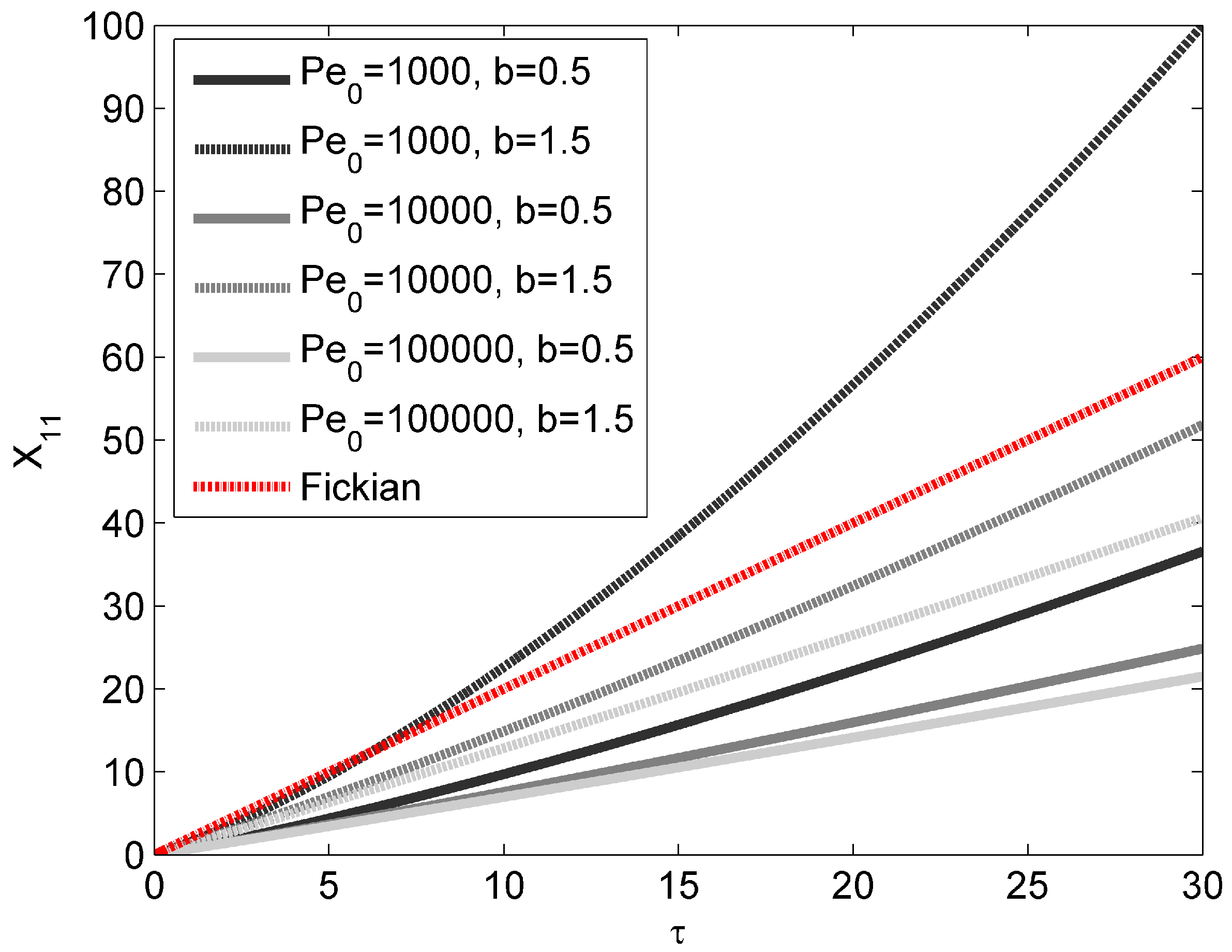
Equations (69) and (72) are graphically represented in Figure 1 and Figure 2, respectively, for $\chi$ = 3 and a travel distance equal to 30l₀. As one can see, the effect produced by high Péclet (Pe₀) numbers is opposite to the effect produced by high scaling exponents (b). Specifically, the higher the Péclet number, the closer the transport process to asymptotic Fickian conditions, represented by a constant longitudinal macro-dispersion coefficient (although, for τ → 0, the dispersion coefficient is higher for higher Péclet numbers due to the larger number of heterogeneity scales initially sampled). Conversely, the higher the scaling exponent, the faster the macro-dispersion coefficient increases. Notice that, in Figure 2, the red dotted line represents the Fickian, linear behavior corresponding to a single-scale log-conductivity field (exponential or Gaussian log-K covariance) characterized by the truncated-hierarchy variance and by an integral scale equal to the initial plume size. Thus, unlike the case of fast-decaying correlation functions, the coexistence of evolving-scale advective heterogeneity and intensive diffusive mixing acts as an antagonist mechanism in the process of solute dilution and Fickian regime achievement. Such a behavior, which is in definite contrast with what was previously found for stationary porous media, was detected here for the first time.

4. Discussion and Conclusions

The present study has shown that the dispersion of solutes in evolving-scale heterogeneous porous formations represented by power-law semi-variograms can be ergodic and Fickian or non-ergodic and super-diffusive, based on the magnitude of the Péclet number, where the Péclet number is intended as the ratio of the product of the ensemble mean velocity and the initial plume size to the local dispersion coefficient, and the scaling exponent value.

Specifically, the larger the Péclet number, the closer the transport process to asymptotically ergodic-Fickian conditions. Conversely, the higher the scaling exponent, the closer the transport process to a non-ergodic super-diffusive regime. In the limit for Péclet tending to infinity (negligible local dispersion), transport is always asymptotically Fickian (regardless of the scaling exponent), with the longitudinal macro-dispersion coefficient that increases with the initial plume size and scaling exponent.

The most important result is that, whereas in weakly heterogeneous formations characterized by short-range correlation functions the local dispersive/diffusive transport mechanisms enhance solute mixing and dilution by a faster achievement of Fickian conditions, the opposite happens in the case of heterogeneous porous formations characterized by persistent correlations represented by power-law semi-variograms.

This result is different from what has been found by previous studies on the same topic. Dagan [13] predicted invariably non-ergodic conditions (the uncertainty related to the centroid location, which is directly dependent on the incomplete dilution, never decayed) and adopted the effective macro-dispersion coefficient as representative of longitudinal dispersion. Dispersion turned out to be asymptotically Fickian for 0 < b < 1 and anomalous for 1 ≤ b < 2. On the other hand, Suciu et al. [18] did not deal with ergodicity issues, defined the macro-dispersion coefficient as one-half of the time-derivative of the particle trajectory covariance X₁₁, and detected invariably super-diffusive regimes.

The different conclusions reached by the present study come from the acknowledgement of the effective-heterogeneity frequencies selection imposed by the finite initial plume size in such very peculiar hydraulic conductivity fields. Practically speaking, the present study recognizes that, in these cases, it is the initial dilution degree that plays a crucial role in terms of further possible dilution.

Indeed, a very concentrated solute spot in high-Péclet number transport processes would remain a very concentrated solute spot at any time: in the presence of long-range log-K correlations, a small solute body does not intercept a band of heterogeneity frequencies sufficient to induce solute dispersion about the center of mass. Conversely, the presence of a non-negligible local dispersive contribution would determine a continuous though slow involvement of larger heterogeneity scales, with the band of effective frequencies that becomes wider and wider. In these conditions, the evolving cut-off would tend to become ineffective in that all scales of heterogeneity would gradually affect both the macro-dispersion coefficient and the uncertainty related to the centroid location. In both cases, however, transport would be non-ergodic:

$$\frac{d\langle S_{11}\rangle }{dt}\ne \frac{d{\tilde{X}}_{11}}{dt}$$

(74)

and anomalous. In the first case, Pe → ∞ and there is no frequency selection due to the infinitesimal plume size:

$$\frac{d\langle S_{11}\rangle }{dt}=\frac{d{X}_{11}}{dt}-\frac{d{R}_{11}}{dt}=0$$

(75)

In the second case, Pe is finite and the frequencies cut off is mobile:

$$\frac{d\langle S_{11}\rangle }{dt}=\frac{d{\tilde{X}}_{11}}{dt}-\frac{d{\tilde{R}}_{11}}{dt}+2D\ne 0$$

(76)

Only with a finite initial plume size (already diluted solute) and negligible local dispersion, one would recover asymptotically ergodic conditions:

$$\frac{d\langle S_{11}\rangle }{dt}\to \frac{d{\tilde{X}}_{11}}{dt}$$

(77)

and a Fickian regime:

$$\frac{d{\tilde{X}}_{11}}{dt}\to 2D_{m11}=\mathrm{const}$$

(78)

Since local dispersion is related to laboratory-scale formation structure, the local analysis of long-range correlation porous media is a crucial issue in predicting the fate of fluids or pollutants subject to release and migration through them. Additionally, it must be emphasized that the linear treatment of flow and transport may hide some relevant second-order effects such as those coming from the interplay of the heterogeneity scales allowed by the complete solution of the flow equation (see Equation (21)) and from the Lagrangian solution of transport based on the complete integro-differential Equation (32), instead of on its linearized version:

$$X^{\prime }\left(t,a\right)\cong {\displaystyle \underset{0}{\overset{t}{\int }}{v}^{\prime }\left[a+U\tau +X_B\left(\tau \right)\right]d\tau }$$

(79)

Finally, provided that any numerical approach would be to some extent biased by the dimensions of the computational domain, it would be desirable that field experiments in highly heterogeneous and complex porous formations validate the theoretical conclusions.

References

- Dagan, G. Flow and Transport in Porous Formations; Springer: Berlin, Germany, 1989; p. 465. [Google Scholar]
- Gelhar, L.W. Stochastic Subsurface Hydrology; Prentice Hall: Upper Saddle River, NJ, USA, 1993; p. 390. [Google Scholar]
- Neuman, S.P. Universal scaling of hydraulic conductivities and dispersivities in geologic media. Water Resour. Res. 1990, 26, 1749–1758. [Google Scholar] [CrossRef]
- Feder, J. Fractals; Plenum Press: New York, NY, USA, 1988; p. 283. [Google Scholar]
- Fischer, H.B.; List, J.E.; Koh, C.R.; Imberger, J.; Brooks, N.H. Mixing in Inland and Coastal Waters; Academic Press: San Diego, CA, USA, 1979; p. 483. [Google Scholar]
- Kitanidis, P.K. Prediction by the method of moments of transport in heterogeneous formation. J. Hydrol. 1988, 102, 453–473. [Google Scholar] [CrossRef]
- Dagan, G. Transport in heterogeneous porous formations: Spatial moments, ergodicity, and effective dispersion. Water Resour. Res. 1990, 26, 1281–1290. [Google Scholar] [CrossRef]
- Rajaram, H.; Gelhar, L.W. Plume scale-dependent dispersion in heterogeneous aquifers: 2. Eulerian analysis and three-dimensional aquifers. Water Resour. Res. 1993, 29, 3261–3276. [Google Scholar] [CrossRef]
- Glimm, J.; Lindquist, W.B.; Pereira, F.P.; Zhang, Q. A theory of macrodispersion for the scale-up problem. Transp. Porous Med. 1993, 13, 97–122. [Google Scholar] [CrossRef]
- Pannone, M. Transient Hydrodynamic Dispersion in Rough Open Channels: Theoretical Analysis of Bed-Form Effects. J. Hydraul. Eng. 2010, 136, 155–164. [Google Scholar] [CrossRef]
- Pannone, M. Longitudinal Dispersion in River Flows Characterized by Random Large-Scale Bed Irregularities: First-Order Analytical Solution. J. Hydraul. Eng. 2012, 138, 400–411. [Google Scholar] [CrossRef]
- Pannone, M. On the exact analytical solution for the spatial moments of the cross-sectional average concentration in open channel flows. Water Resour. Res. 2012, 48, W08511. [Google Scholar] [CrossRef]
- Dagan, G. The significance of heterogeneity of evolving scales and of anomalous diffusion to transport in porous formations. Water Resour. Res. 1994, 30, 3327–3336. [Google Scholar] [CrossRef]
- Bellin, A.; Pannone, M.; Fiori, A.; Rinaldo, A. On transport in porous formations characterized by heterogeneity of evolving scales. Water Resour. Res. 1996, 32, 3485–3496. [Google Scholar] [CrossRef]
- Edery, Y.; Guadagnini, A.; Scher, H.; Berkowitz, B. Origins of anomalous transport in heterogeneous media: Structural and dynamical controls. Water Resour. Res. 2014, 50, 1490–1505. [Google Scholar] [CrossRef]
- Kang, P.K.; Brown, S.; Juanes, R. Emergence of anomalous transport in stressed rough fractures. Earth Planet. Sci. Lett. 2016, 454, 46–54. [Google Scholar] [CrossRef]
- Wang, L.; Cardenas, M.B. Transition from non-Fickian to Fickain longitudinal transport through 3-D rouogh fractures: Scale-(in)sensitivity and roughness dependence. J. Contam. Hydrol. 2017, 198, 1–10. [Google Scholar] [CrossRef] [PubMed]
- Suciu, N.; Attinger, S.; Radu, F.A.; Vamos, C.; Vanderborght, J.; Vereecken, H.; Knauber, P. Solute transport in aquifers with evolving scale heterogeneity. Versita 2015, 23, 167–186. [Google Scholar] [CrossRef]
- Gelhar, L.W. Stochastic subsurface hydrology from theory to applications. Water Resour. Res. 1986, 22, 135S–145S. [Google Scholar] [CrossRef]
- Frampton, A.; Cvetkovic, V. Significance of injection modes and heterogeneity on spatial and temporal dispersion of advecting particles in two-dimensional discrete fracture networks. Adv. Water Resour. 2009, 32, 649–658. [Google Scholar] [CrossRef]
- Kang, P.K.; Dentz, M.; Le Borgne, T.; Lee, S.; Juanes, R. Spatial Markov model for dispersion with variable injection modes. Adv. Water Resour. 2017, 106, 80–94. [Google Scholar] [CrossRef]
- Hyman, J.D.; Painter, S.L.; Viswanathan, H.; Makedonska, N.; Karra, S. Influence of injection mode on transport properties kilometer-scale three-dimensional discrete fracture networks. Water Resour. Res. 2015, 51, 7289–7308. [Google Scholar] [CrossRef]
- Demmy, G.; Berglund, S.; Graham, W. Injection mode implications for solute transport in porous media: Analysis in a stochastic Lagrangian framework. Water Resour. Res. 1999, 35, 1965–1973. [Google Scholar] [CrossRef]
- Dentz, M.; Kang, P.K.; Comolli, A.; Le Borgne, T.; Lester, D.R. Continuous time random walks for the evolution of lagrangian velocities. Phys. Rev. Fluid. 2016, 1, 074004. [Google Scholar] [CrossRef]
- Pannone, M.; Kitanidis, P.K. Large-time behavior of concentration variance and dilution in heterogeneous formations. Water Resour. Res. 1999, 35, 623–634. [Google Scholar] [CrossRef]
- Pannone, M. Effect of nonlocal transverse mixing on river flows dispersion: A numerical study. Water Resour. Res. 2010, 46, W08534. [Google Scholar] [CrossRef]
- Pannone, M. Predictability of tracer dilution in large open channel flows: Analytical solution for the coefficient of variation of the depth-averaged concentration. Water Resour. Res. 2014, 50, 2617–2635. [Google Scholar] [CrossRef]
- Gradshteyn, I.S.; Ryzhik, I.M. Table of Integrals, Series, and Products, 5th ed.; Academic Press: San Diego, CA, USA, 1994; p. 1204. [Google Scholar]
- Pannone, M.; Kitanidis, P.K. On the asymptotic behavior of dilution parameters for Gaussian and Hole-Gaussian log-conductivity covariance functions. Transp. Porous Med. 2004, 56, 257–281. [Google Scholar] [CrossRef]
Figure 1.
Longitudinal macro-dispersion coefficient for variable Péclet numbers and scaling exponents.
Figure 2.
Longitudinal particle trajectory covariance for variable Péclet numbers and scaling exponents. The red-dotted line refers to Fickian linear behavior corresponding to a single-scale log-conductivity field (exponential or Gaussian log-K covariance) characterized by the truncated-hierarchy variance and by an integral scale equal to the initial plume size.
© 2017 by the author. Licensee MDPI, Basel, Switzerland. This article is an open access article distributed under the terms and conditions of the Creative Commons Attribution (CC BY) license (http://creativecommons.org/licenses/by/4.0/).
Share and Cite
MDPI and ACS Style
Pannone, M. An Analytical Model of Fickian and Non-Fickian Dispersion in Evolving-Scale Log-Conductivity Distributions. Water 2017, 9, 751. https://doi.org/10.3390/w9100751
AMA Style
Pannone M. An Analytical Model of Fickian and Non-Fickian Dispersion in Evolving-Scale Log-Conductivity Distributions. Water. 2017; 9(10):751. https://doi.org/10.3390/w9100751
Chicago/Turabian StylePannone, Marilena. 2017. "An Analytical Model of Fickian and Non-Fickian Dispersion in Evolving-Scale Log-Conductivity Distributions" Water 9, no. 10: 751. https://doi.org/10.3390/w9100751
Note that from the first issue of 2016, this journal uses article numbers instead of page numbers. See further details here.