Application of a Hybrid Interpolation Method Based on Support Vector Machine in the Precipitation Spatial Interpolation of Basins

1
State Key Laboratory of Hydraulics and Mountain River Engineering, College of Water Resource and Hydropower, Sichuan University, Chengdu 610065, China
2
Three Gorges Cascade Dispatching & Communication Center, Yichang 443133, China
*
Author to whom correspondence should be addressed.
Water 2017, 9(10), 760; https://doi.org/10.3390/w9100760
Submission received: 23 August 2017
/
Revised: 24 September 2017
/
Accepted: 26 September 2017
/
Published: 2 October 2017
Abstract
:In this paper, we applied the support vector machine (SVM) to the spatial interpolation of the multi-year average annual precipitation in the Three Gorges Region basin. By combining it with the inverse distance weighting and ordinary kriging method, we constructed the SVM residual inverse distance weighting, as well as the SVM residual kriging precipitation interpolation model and compared them with the inverse distance weighting, ordinary kriging, linear regression residual inverse distance weighting and linear regression residual kriging interpolation methods. The TRMM 3B43 V7 satellite precipitation information, which is processed by the latest revision algorithm, is used as the auxiliary variable for ground site precipitation interpolation along with latitude and elevation. Our results show that: (1) adding the TRMM 3B43 V7 satellite precipitation data as an auxiliary variable significantly improves the interpolation accuracy of the linear regression equation and SVM model; (2) the support vector machine hybrid interpolation method obtains superior interpolation results compared to the inverse distance weighting method, ordinary kriging method and linear regression hybrid interpolation method; (3) the interpolation accuracy of the SVM hybrid interpolation method depends on the SVM fitting degree, so we should choose a suitable fitting accuracy rather than the highest fitting accuracy; (4) the linear regression equation has a greater degree of dependency on the TRMM data than the SVM. The SVM accepts the TRMM data information while better maintaining its independence, taking into account that the TRMM data linear regression and linear regression hybrid interpolation method are not suitable for TRMM data evaluation.
1. Introduction
Rainfall is the most active factor in the water cycle of basins. It plays an essential role in the formation of runoff. Research on the spatial interpolation of rainfall can facilitate the acquisition of the spatial distribution characteristics of rainfall, which have great significance for the analysis of basin water status, water resources management, drought and flood disaster prediction and hydrological ecological simulation [1]. The commonly-used precipitation interpolation methods can be divided into two categories: global interpolation methods (e.g., trend surface method and multiple regression method) and local interpolation methods (e.g., inverse distance weighting method and kriging method) [2,3]. The difference is whether the method uses all the site precipitation data in the study area or only the site precipitation data in the local area of the study area to predict the unknown sample. The global interpolation method and local interpolation method are combined to form a hybrid interpolation method (e.g., linear regression residual kriging, linear regression residual inverse distance weighting), and the interpolation accuracy is further improved by correcting the residuals in the global interpolation method.
Originally, SVM was designed for pattern recognition. Later, with the introduction of insensitive loss functions, SVM also showed good learning performance in regression estimation of nonlinear systems. In recent years, SVM has been widely applied to the fields of hydrology [4,5,6,7], meteorology [8,9] and water environment [10], etc., as well as research on spatial interpolation. In spatial interpolation with SVM, by learning of known samples, non-linear relationships between data and properties are approached to realize the forecast of unknown samples. At present, the research concerning SVM in spatial interpolation mainly focuses on the following three aspects. First, it aims to improve the existing interpolation method by using the SVM. Huang et al. (2012) proposed a kriging interpolation method based on the SVM, using it to directly fit the optimal semi-variance function and then the kriging interpolation, to avoid subjectivity in the semi-variance model selection process [11]. This method is applied to the restoration of missing marine data, and the interpolation effect is better than that of the ordinary kriging method. Second, the SVM is used to simulate and predict the spatial distribution of variables. Gilardi and Bengio (2009) explored the feasibility and significance of machine learning methods for nonstationary spatial data analysis. They studied two types of global models (support vector regression and multilayer perceptrons) and two types of local models (a local version of support vector regression and mixture of experts) and conducted the Spatial Interpolation Comparison 97 experiment to predict the rainfall of unknown samples. The results show that the local model gives a better interpolation effect [12]. Li et al. (2011) established a model of SVM, ore-grade interpolation based on the cross-validation method, transforming the problem of spatial interpolation into the problem of solving a nonlinear function between mineral grade and its influencing factors [13]. In addition, the SVM is also applied to the accumulated temperature, elevation and other variable spatial interpolation [14,15]. Third, a new hybrid interpolation method is proposed by combining the SVM with inverse distance weighting, ordinary kriging and other local interpolation methods. Li et al. (2011) used SVM, ordinary kriging, inverse distance squared and their combinations to conduct spatial interpolation of mud content samples in the southwest Australian margin; however, the SVM and its combination with ordinary kriging or inverse distance squared are not suitable for the spatial interpolation effect of mud content in this region [16]. The interpolation precision of SVM is affected by normalization range, the selection of kernel functions and the reasonable setting of the insensitive loss parameter and penalty parameter, etc. As model parameters are given arbitrarily or given in accordance with testing experience, their large randomness and uncertainty impact the prediction precision to some extent.
On the whole, SVMs are less often used in spatial interpolation. First, because of the inverse distance weighting, ordinary kriging and other commonly-used interpolation methods are simpler than the SVM method, while their interpolation precision is stable and their versatility strong. Second, the SVM is a machine learning method, and although there is a mathematical foundation, it still functions as a black box. The explanation of its functioning needs to be improved. However, SVMs are an option when the study area does not permit commonly-used interpolation methods or when these methods cannot meet the requirements of interpolation [12]. With reasonable selection of input variables and model parameters, SVMs can achieve the desired predictive results.
There are many factors that affect the spatial distribution of precipitation, including the longitude, latitude, elevation, slope and aspect of the station. In addition, Zhu and Huang (2007) proposed the highest elevation within 3 km of the site and the distance to Thousand-Islet Lake as a precipitation influencing factor [17]; Sun et al. (2015) considered the surface roughness and river network density factor [18]; Bostan et al. (2012) took the distance to the nearest coast, land cover and eco-region as precipitation interpolation auxiliary variables [19]; Seo et al. (2015) included the distance to the summit of the Halla Mountain and the distance to the coastline into the calculation [20]; temperature, wind speed and other variables also have a certain degree of impact on the precipitation. Taking the various factors that affect precipitation into consideration is helpful to improve the interpolation precision, but one should not think that the more factor choices there are, the better the interpolation effect is. It is particularly important to choose a key factor that reflects the characteristics of precipitation in the study area.
In recent years, a series of high-resolution satellite remote sensing precipitation products has provided a new source of data for global and regional precipitation observations that are widely used in the field of hydrometeorology [21,22,23,24]. Although satellite precipitation products have some deviation, they are spatially distributed to compensate for the lack of site observations [25]. Satellite precipitation products can be used as an auxiliary variable for ground site precipitation interpolation in order to improve the accuracy of precipitation interpolation. The TRMM (Tropical Rainfall Measuring Mission satellite) 3B42/3B43 data are widely used, usually combined with co-kriging, simple kriging with locally varying mean, regression kriging, kriging with an external drift and other methods, to interpolate the ground site’s daily, monthly, annual and other multi-scale precipitation [26,27,28,29]. Improving interpolation accuracy often depends on the accuracy of the TRMM data in the study area. If the TRMM data of the study area are correlated with the measured data of the ground station, the interpolation method of adding the TRMM data as the auxiliary variable often achieves the ideal interpolation effect.
In this study, we used TRMM 3B43 V7 precipitation products, together with latitude and elevation as ground site precipitation interpolation auxiliary information and built the SVM, the SVM residual inverse distance weighting (SVMRI) and the SVM residual kriging (SVMRK) precipitation interpolation model. We used these in the spatial interpolation calculations of the Three Gorges Region multi-year average annual precipitation (P) and compared with the inverse distance weighting (IDW), ordinary kriging (OK), linear regression residual inverse distance weighting (LRI) and linear regression residual kriging (LRK) methods.
2. Study Basin and Data
2.1. Research Basin
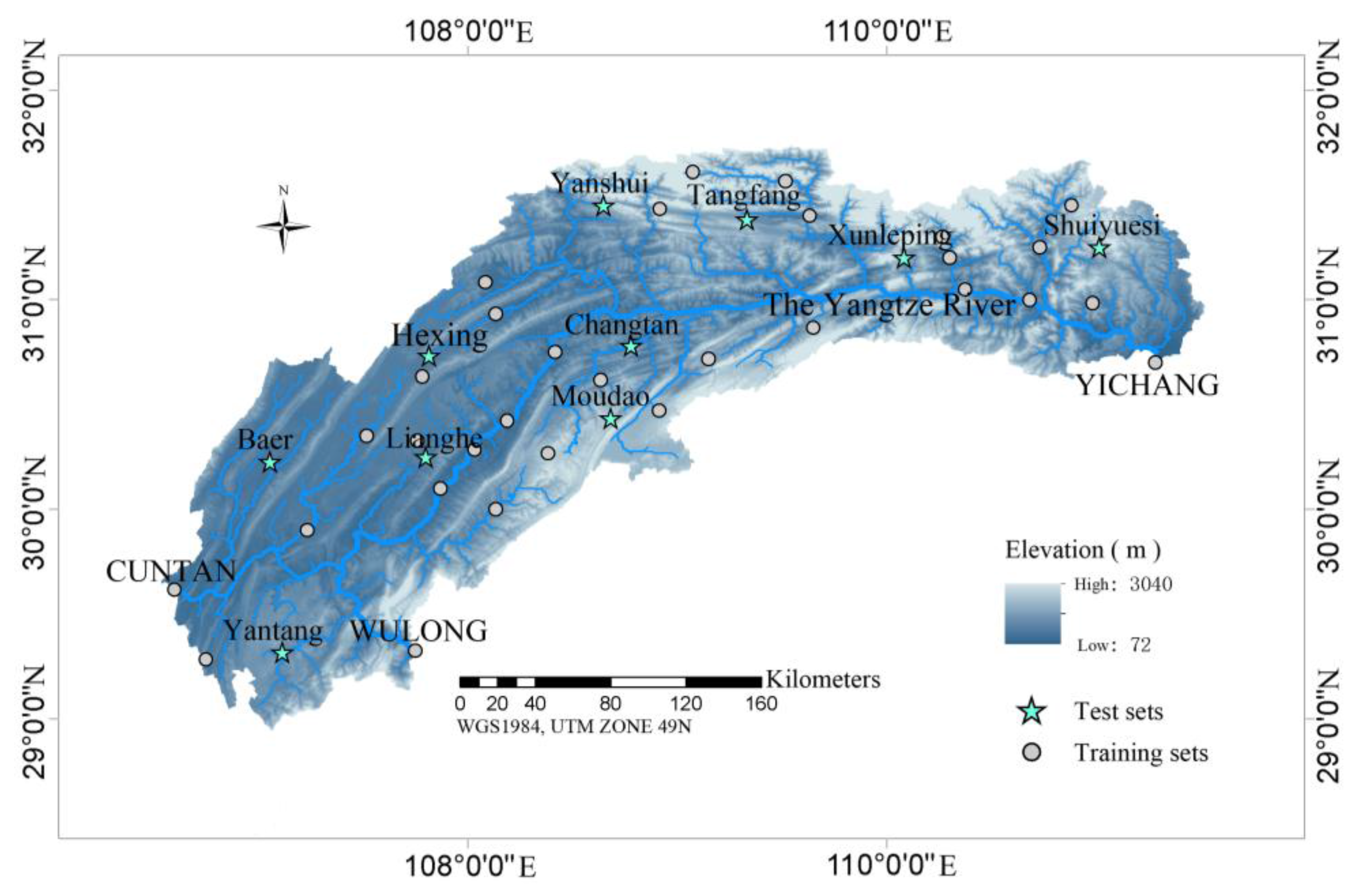
This study focused on the Three Gorges Region basin between the Cuntan hydrological station along the main stream of the Yangtze River and the Wulong hydrological station along the Yangtze River tributary, Wu Jiang River. The water area of the Three Gorges Region is approximately 60,000 km2. The total length of the main stream is 658 km. It is located at east longitude between 106°36′00″ and 110°44′00″ and north latitude between 28°56′00″ and 31°44′18″. The terrain and geomorphologic conditions in the area are complex, and the higher western section of Fengjie is the low elevation area of the Sichuan Basin. The lower eastern section of Fengjie is the canyon alpine area, and the tributaries are relatively short. The climate in the basin area is in a transition zone from north temperate to subtropical monsoon. Because of the canyon terrain, the eastern and western climates are quite different. The south and north shores are located in the heavy rainstorm range of the southwestern Hubei and the Daba Mountains in the Yangtze River basin [30]. Heavy, high-intensity rain occurs frequently, with heavy rainstorms mostly moving from the west to the east, downstream along the main stream.
2.2. Research Data
2.2.1. Ground Observation Data
The Three Gorges Project began construction in 1994, and the main dam was completed in 2006. This study collected the monthly precipitation data of 41 ground rainfall stations from 2006–2016 in the Three Gorges Region. The data were derived from the water-rain-situation telemetry system of China Three Gorges Corporation. We randomly selected 31 sites as interpolation training stations and 10 sites as test stations, using the site distribution shown in Figure 1, and took the multi-year average annual precipitation from 2006–2016 as the interpolation objects.
2.2.2. TRMM 3B43 V7 Satellite Precipitation Data
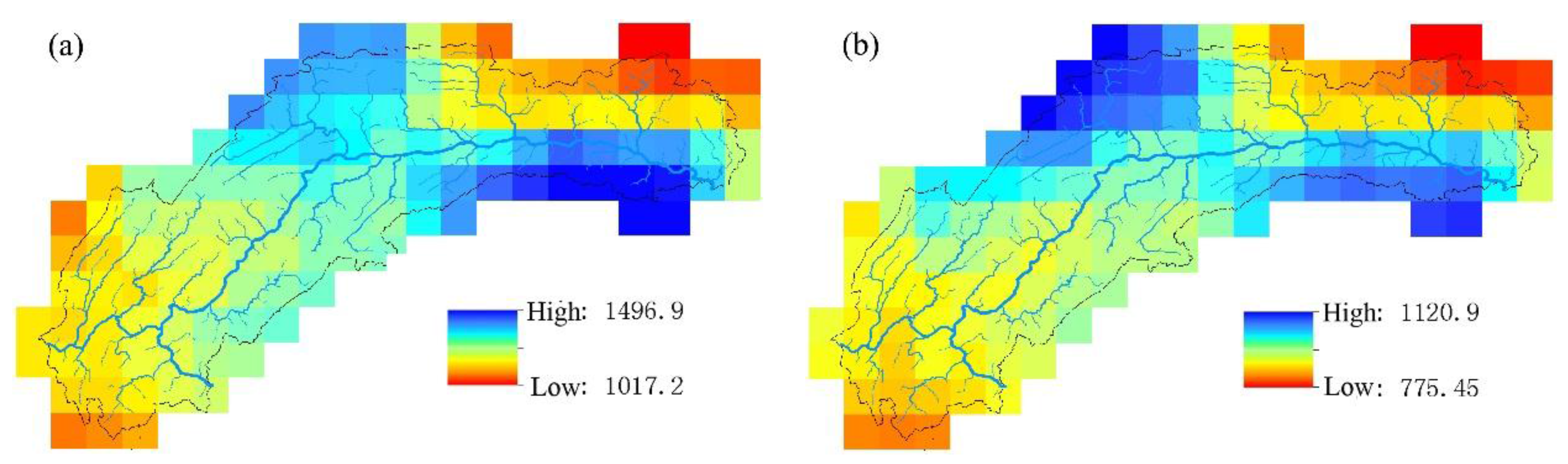
The study also collected TRMM 3B43 V7 global precipitation data. 3B43 V7 was improved compared to 3B43 V6 [31], covering a range of 50° N–50° S and 180° W–180° E with a spatial resolution of 0.25° × 0.25° and a time resolution of a month. The 3B43V7 data used in this study were downloaded from the Precipitation Measurement Missions (PMM) website (http://pmm.nasa.gov/data-access/downloads/trmm). The monthly TRMM data of the Three Gorges Region was extracted from 2006–2016, and the annual precipitation of the Three Gorges Region and the precipitation in the flood season (May–October) were calculated and averaged over these years (Figure 2).
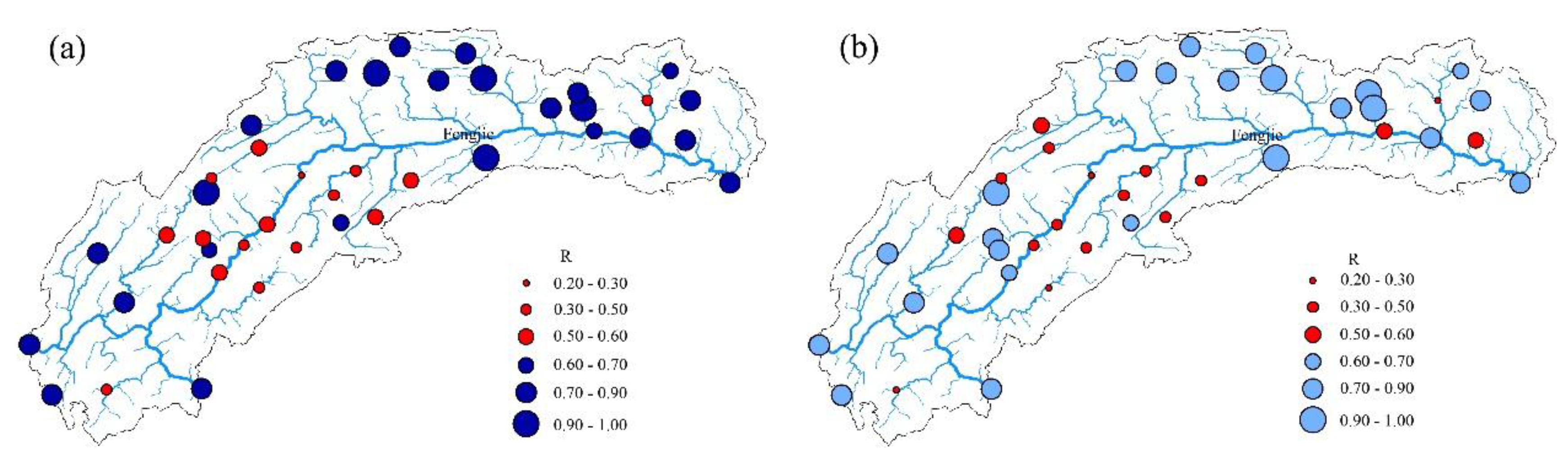
We carried out the correlation analysis between the observation sequence of precipitation in the year, as well as the flood season of the study area and the corresponding grid of TRMM data sequences, verifying the correlation degree of satellite data and ground observation data. The spatial distribution of the correlation coefficient between the year and flood season is shown in Figure 3, with the red site correlation coefficient not passing the significance test. The figure shows that the terrain of the Three Gorges Region above Fengjie is relatively flat, showing a small correlation coefficient, while the terrain of the basin below Fengjie is alpine canyon, and the correlation coefficient is big.
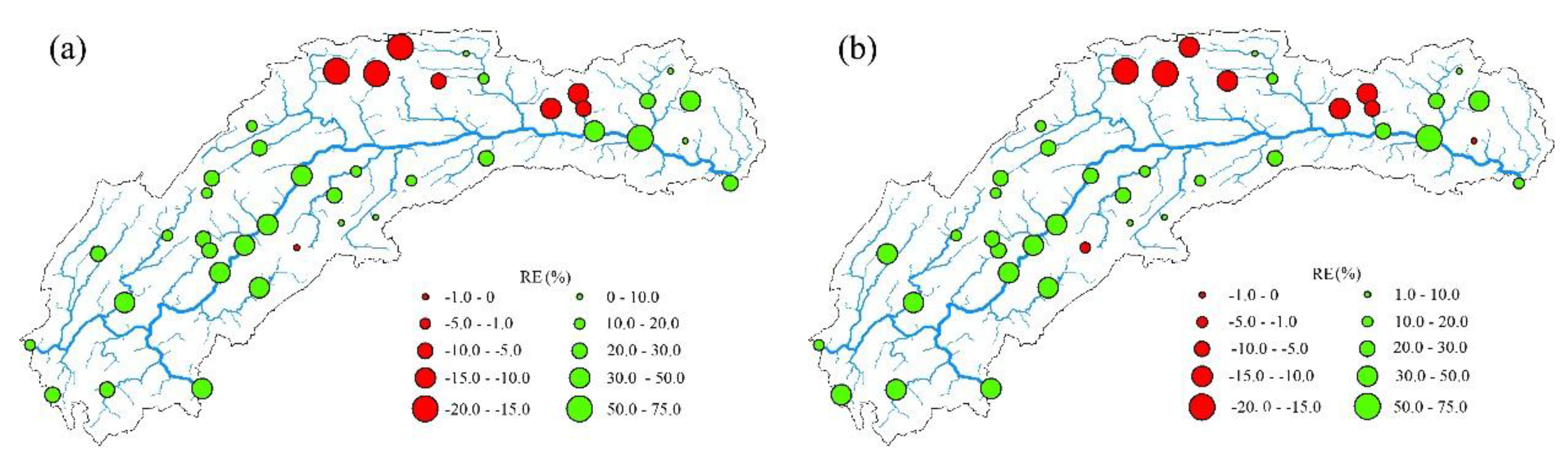
The multi-year average annual precipitation of 41 sites is 1110.54 mm, and the corresponding TRMM multi-year average annual precipitation is 1270.54 mm, the overall value being 14.40% higher than the measured value. The multi-year average annual precipitation of 41 sites is 851.88 mm in the flood season, and the corresponding TRMM multi-year average annual precipitation is 963.60 mm, the overall value being 13.11% higher than the measured value. The relative error (RE) of each site is shown in Figure 4.
Overall, the TRMM 3B43 V7 satellite data and the ground observation data of the Three Gorges Region have significant time correlation in most of the stations on the scale of year and flood season, although for some sites, the time correlations are not significant, these being concentrated in the flat terrain above the Fengjie area. The TRMM data deviate from ground site precipitation: the overall value is too large, and the values of precipitation-rich centers are too small. TRMM data detect the basin precipitation-rich center locations relatively accurately, showing good spatial distribution continuity, making up for the shortcoming that the number of local ground sites is insufficient or the distribution is unreasonable.
2.3. Interpolation Auxiliary Variable Selection
Geographic location and topographic features are important factors influencing the spatial distribution of precipitation. In this paper, the site longitude (X), latitude (Y), slope (S), aspect (A), elevation (E) and the maximum elevation within a 10-km range (E10) were taken as interpolation auxiliary variables. Compared with the measured precipitation data, the TRMM satellite precipitation data better reflect the spatial distribution characteristics of the precipitation, although there is a certain degree of deviation in its accuracy. We also included the TRMM satellite precipitation data in the auxiliary variables, including the TRMM multi-year average annual precipitation (T) and multi-year average flood season precipitation (Tfs), in order to improve the accuracy of site precipitation.
The correlation between the auxiliary variables and multi-year average annual precipitation from 2006–2016 is shown in Table 1. After comprehensively considering the Pearson correlation coefficient and Spearman correlation coefficient, we chose Y, E, E10, T and Tfs as interpolation auxiliary variables, but E and E10, T and Tfs were not used as auxiliary variables at the same time.
3. Research Methods
3.1. Commonly-Used Interpolation Methods
The inverse distance weighting method and ordinary kriging method are the most commonly-used interpolation methods [32,33]. The inverse distance weighting method is based on the similarity of the region and predicts the precipitation of unknown samples by weighting the adjacent stations. The ordinary kriging method is the unbiased optimal estimation of the spatial distribution of precipitation in the study area based on the statistical characteristics of known site precipitation. The inverse distance weighting method and the kriging interpolation method belong to the local weighted average interpolation methods, but the weight determination method is different: the inverse distance weighting method determines the weight by the distance between the unknown point and the measured site, while the kriging interpolation method, to satisfy the unbiased optimal condition, uses the Lagrangian multiplier to find the minimum and solves the weight value of each measured station using the semi-variance value.
3.2. Linear Regression Hybrid Interpolation Method
Vicente-Serrano et al. (2003) proposed for the first time to combine the regression model with deterministic methods or geostatistical interpolation to form a hybrid interpolation method [34]. This method first establishes the regression equation between the auxiliary variable and target variable, then predicts the target variable using the regression equation. It calculates the residuals of the target variable and after interpolating the residual, superimposes the residual interpolation data on the regression value of the target variable to obtain a new prediction value. The method assumes that the regression residual preserves the spatial structure inherent in the target variable, which is only valid when the spatial correlation of the residual is obvious.
In this study, we selected auxiliary variables such as latitude, elevation and TRMM satellite precipitation data and established the regression equation with the average annual precipitation of 2006–2016, as shown in Table 2.
The spatial autocorrelation analysis of the regression residuals shows that the four sets of regression residuals have strong spatial autocorrelation. The inverse distance weighting method and ordinary kriging method are used to interpolate the residuals, respectively.
3.3. Support Vector Machine Interpolation Model
3.3.1. Methodology
The SVM is based on the principle of Vapnik-Chervonenkis dimension (VC dimension) and the minimum structure risk in statistical learning theory, seeking the best compromise between complexity and learning ability according to the limited sample information in order to obtain the best predication performance. The SVM is developed from the optimal classification faces in a linear separable situation. The optimal classification face not only separates the two types of samples correctly, but also makes the classification interval the largest. There is only one type of support vector regression machine sample point. The optimal hyperplane is not the one that puts two types of sample points the farthest from each other, but the one with the minimum “total deviation” of all the sample points from the hyperplane. Finding the optimal regression hyperplane is equivalent to finding the maximum interval.
Support vector regression machine not only solves the linear regression problem, but more importantly, can solve the problem of nonlinear regression. The key is to map the original dataset, as the training set data, into a high-dimensional linear feature space through the nonlinear function and construct the regression estimation function in the linear space where the dimension may be infinite, as shown in Equation (1):
where the training sample set is , l is the training sample length, is the input vector and is the output vector; the dimension of is the feature space dimension.
The optimization problem is:
where is the specified insensitive loss parameter and ; and are the relaxation variables; c is the penalty parameter.
Following the standard derivation, the duality optimization problem is obtained:
where are the Lagrange multipliers.
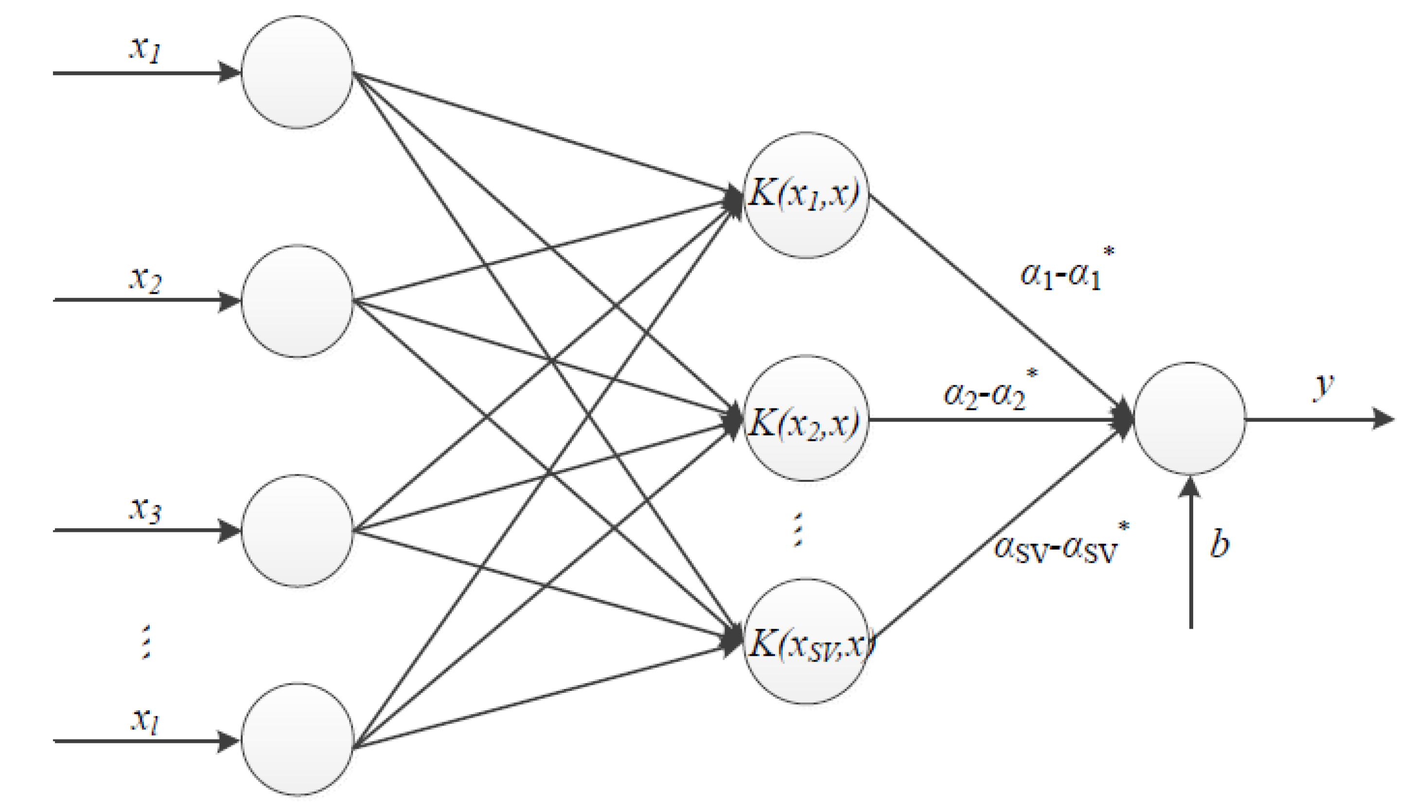
is called the kernel function, and the regression estimation function is:
where the corresponding sample data of comprise the unsupported vector. The corresponding sample data of is the support vector; is called the support value; SV is the number of support vectors; and only the support vector contributes to the estimation function . The structure of the nonlinear SVM is shown in Figure 5.
Although the sample data are mapped to a feature space with a high dimension or even an infinite dimension through a nonlinear function, it does not need to explicitly compute the nonlinear function when calculating the regression estimation function. Only the kernel function is calculated, to avoid the high dimensional disaster problem. The choice of kernel functions must satisfy the Mercer condition. Common kernel functions use linear functions, polynomial functions, radial basis functions and multi-layer perceptron functions. The radial basis function is more versatile, the effect more stable, and it is the most commonly used. It is shown in Equation (5):
where g is a kernel function parameter.
SVM aims at dealing with convex quadratic programming, obtaining globally-optimal solutions and avoiding a local optimum during training. Taking empirical risk minimization as the constraint condition and confidence risk minimization as the optimization objective, SVM reflects good generalization. However, it is difficult to use SVM in large samples, where data storage and calculation will cost much time and memory. On the whole, with a solid theory foundation, SVM is suitable for solving small-sample nonlinear complex problems. Precipitation measurement on ground sites is limited by topography and site distribution; moreover, supplementary information and precipitation show a nonlinear relation. For all the above, SVM is appropriate for solving spatial interpolation of precipitation.
3.3.2. Modeling Steps
Input and Output Selection
According to the screening results of auxiliary variables, we constructed nonlinear regression SVM using the latitude, elevation and satellite precipitation as the input vector and multi-year average annual precipitation of the training station from 2006–2016 as the output target value, and we considered the following six combinations of input vectors: ① Y-E; ② Y-E-T; ③ Y-E-Tfs; ④ Y-E10; ⑤ Y-E10-T; ⑥ Y-E10-Tfs.
Data Normalization
In order to eliminate the dimensional or magnitude differences in dimension data, we must first normalize the data to improve the simulation and prediction accuracy. Different normative ranges have a certain degree of influence on the prediction accuracy of the model [35]. A total of 7 normative ranges of (0, 50), (0, 20), (0, 10), (0, 7), (0, 4), (0, 1), (0.1, 0.9) was selected to process the training and forecast data.
Parameter Initialization
The smaller the insensitive loss parameter , the higher the accuracy of the regression estimation is, but the increase of the number of support vectors may lead to the model being too complicated and without good extrapolation ability. When is bigger, the number of support vectors is small, but the accuracy of the regression estimation is reduced. Based on prior experience, the insensitive loss parameter is set as 0.1.
The penalty parameter c determines the degree of emphasis on the loss of samples other than the insensitive region , which affects the complexity and stability of the model. The form and parameters of the kernel function determine the type and complexity of the regression device, which is an important means to control the performance of the regression device. This study chooses the radial basis kernel function. The parameter in the kernel function controls the radial extent of the function, reflecting the degree of correlation between the support vectors. The penalty parameter c and the kernel function parameter g are usually either given or taken from experience, resulting in great randomness and uncertainty, which will affect the prediction accuracy to a certain extent.
Through the cross-validation (CV) method, we can find the relative best parameters c and g, so that the training set can achieve the highest prediction accuracy under the CV idea. This is calculated by using the K-fold CV method, with K set to 10. The training samples were divided into 10 sets, with the first of each set of data made a test subset and the remaining nine sets accordingly made training subsets. The average over 10 sets of the test subset errors serves as a performance indicator of the model.
In the actual calculation process, the situation of different parameters with the same effect may occur, that is there may be multiple sets of parameters c and g corresponding to the highest prediction accuracy. In this case, we select the parameter set with the smallest c as the best parameter. If there are multiple values of g corresponding to the smallest c, the first sets of c and g identified are selected as the best parameters (a c that is too high will cause the overfitting state to occur). Usually, c and g are in the exponential range of 2 within the grid to discretize the search. The cstep and gstep parameters, the step sizes for the optimization of the c and g cross-validation method, were set to 0.2 in this study.
Construct a Nonlinear Decision Function
Using the training set to solve the optimization problem (Equation (2)), the nonlinear regression estimation function (Equation (4)) is calculated.
Forecast Based on Nonlinear Decision Function
Using the latitude, elevation and satellite precipitation of the test station as the input vector, the precipitation of the test station is predicted by the obtained nonlinear decision function and compared with the measured precipitation.
3.4. Support Vector Machine Hybrid Interpolation Method
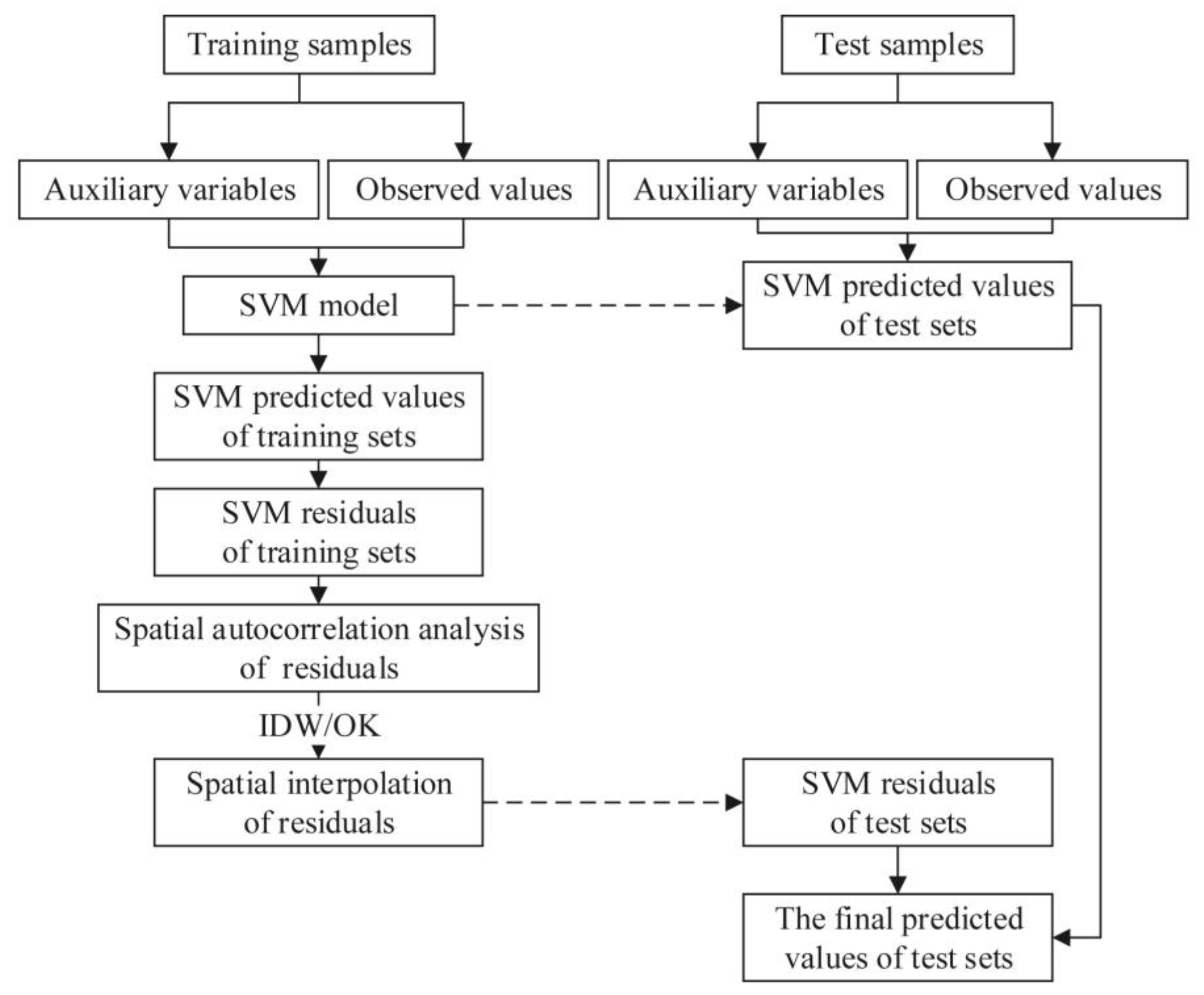
The construction of the SVM model is based on the training station site information and site measured precipitation, which can predict the precipitation of the test station and determine the spatial interpolation of precipitation. At the same time, we conducted the residual calculation and spatial autocorrelation analysis on the training station measured precipitation value and SVM model predictive value. The results suggest that the SVM residuals also show obvious spatial autocorrelation. Therefore, in this study, we further used the inverse distance weighting method and the ordinary kriging method to interpolate the SVM residuals, superimposed the residual interpolation results and SVM predictive results and obtained the final precipitation spatial interpolation results. The SVM residual hybrid interpolation method is shown in Figure 6.
3.5. Error Evaluation Index
Three indexes were used in this study to assess the simulation accuracy of rainfall in test stations.
3.5.1. Root Mean Square Error
The smaller the RMSE, the closer the predicted value to the measured value, and thus, the higher the prediction accuracy.
where is the predicted value, is the measured value and N is the number of stations.
3.5.2. Mean Relative Error
The smaller the MRE, the smaller the predicted error and the higher the prediction accuracy.
3.5.3. Coefficient of Determination (R2)
The closer the R2 is to 1, the better the model fits the data.
where is the mean value of the observed values of the test sample and is the mean value of the test sample.
4. Analysis and Discussion of Results
4.1. Results Analysis
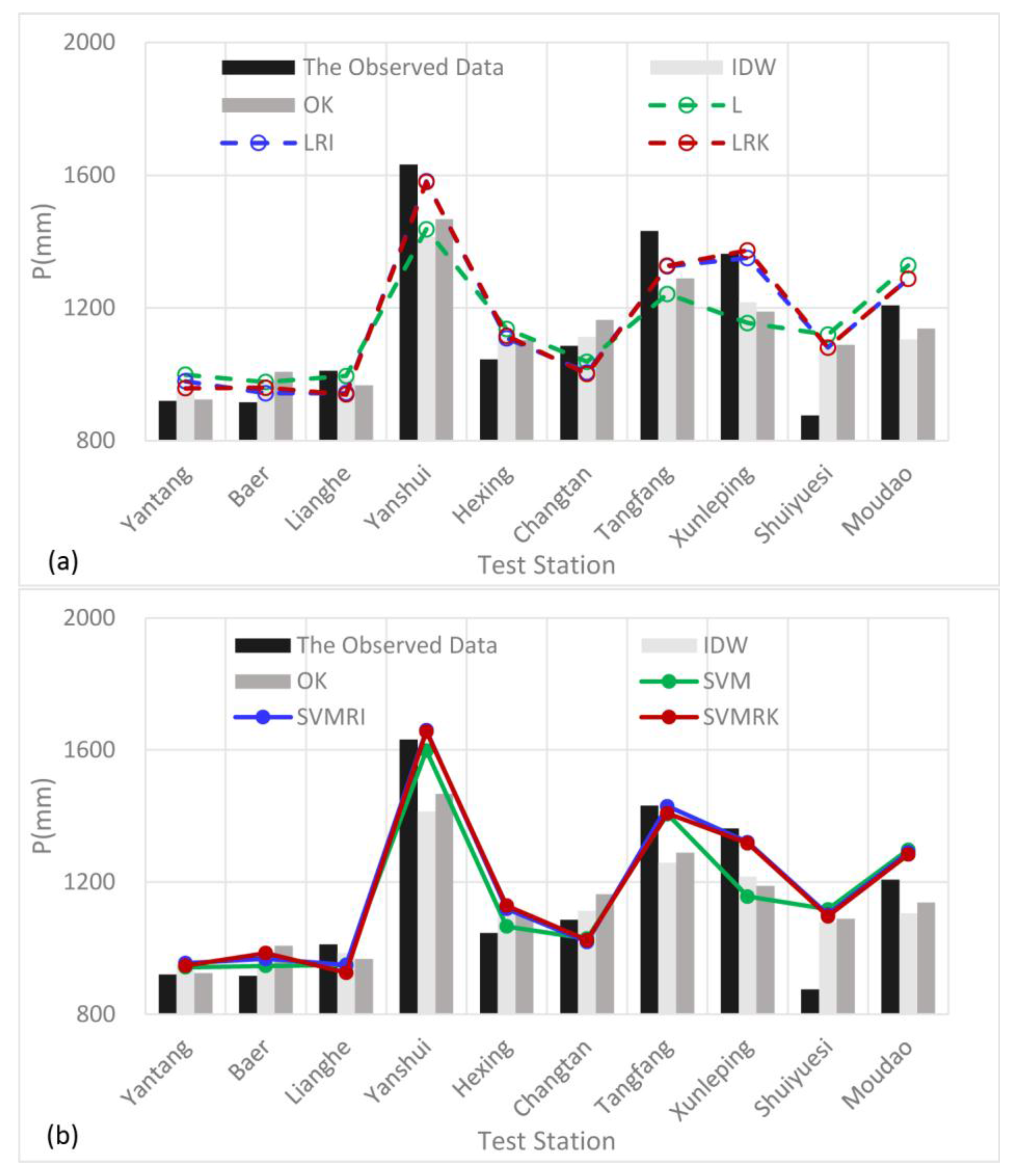
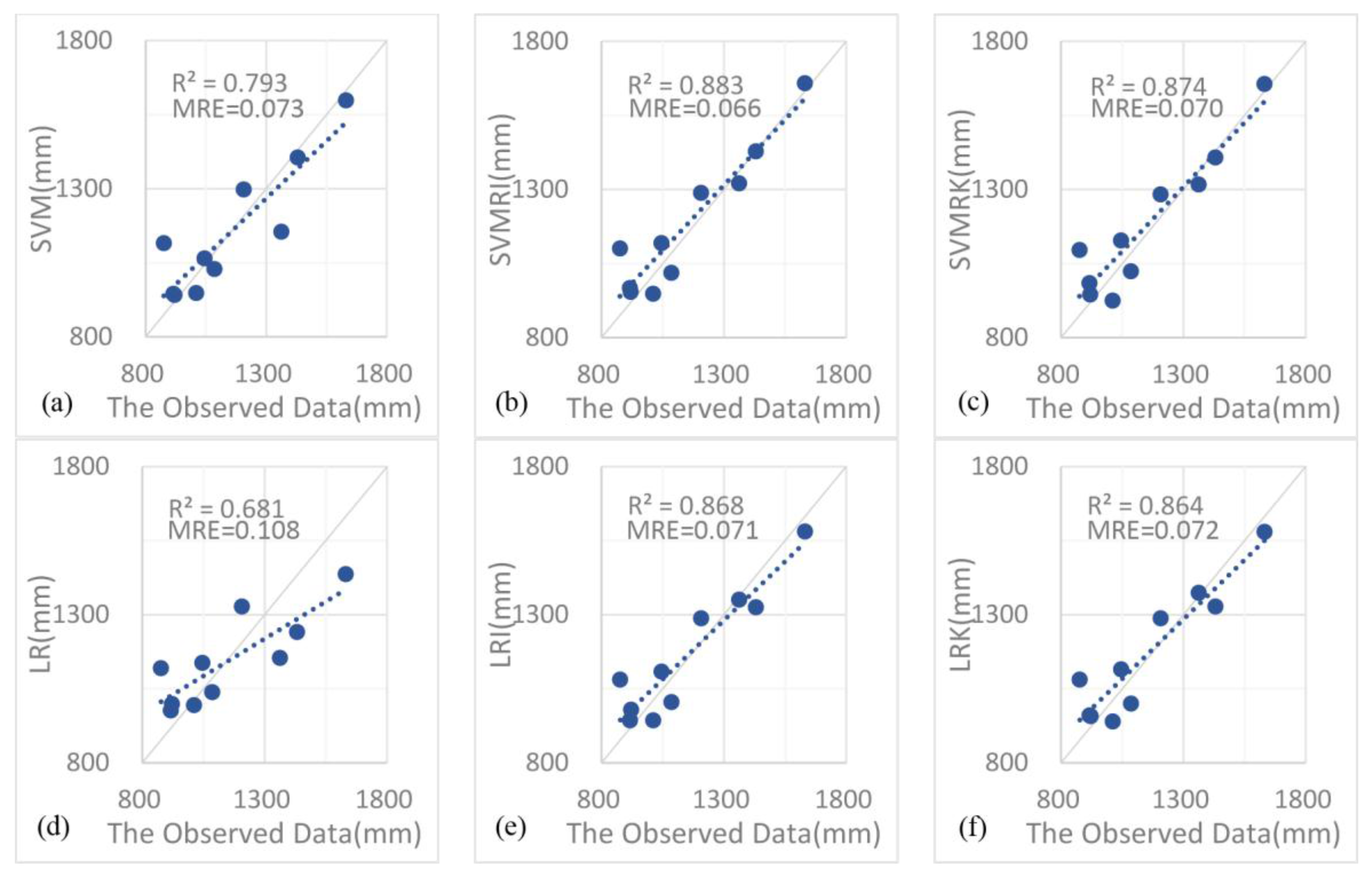
In this study, 31 ground stations were selected as the training stations for the spatial interpolation of precipitation, and the precipitation of 10 stations was predicted and compared with the measured precipitation. The calculation results of the test station error index are shown in Table 3. The precipitation of the test station is shown in Figure 7 and Figure 8. The support vector hybrid interpolation method and linear regression hybrid interpolation method in Figure 7 and Figure 8 are the smallest set of parameter interpolation results from the test set RMSE. The SVM and the linear regression equation correspond to their respective hybrid interpolation methods. At the same time, the spatial distribution of multi-year average annual precipitation with a spatial resolution of 0.25° × 0.25° is obtained through interpolation in the Three Gorges Region (Figure 9).
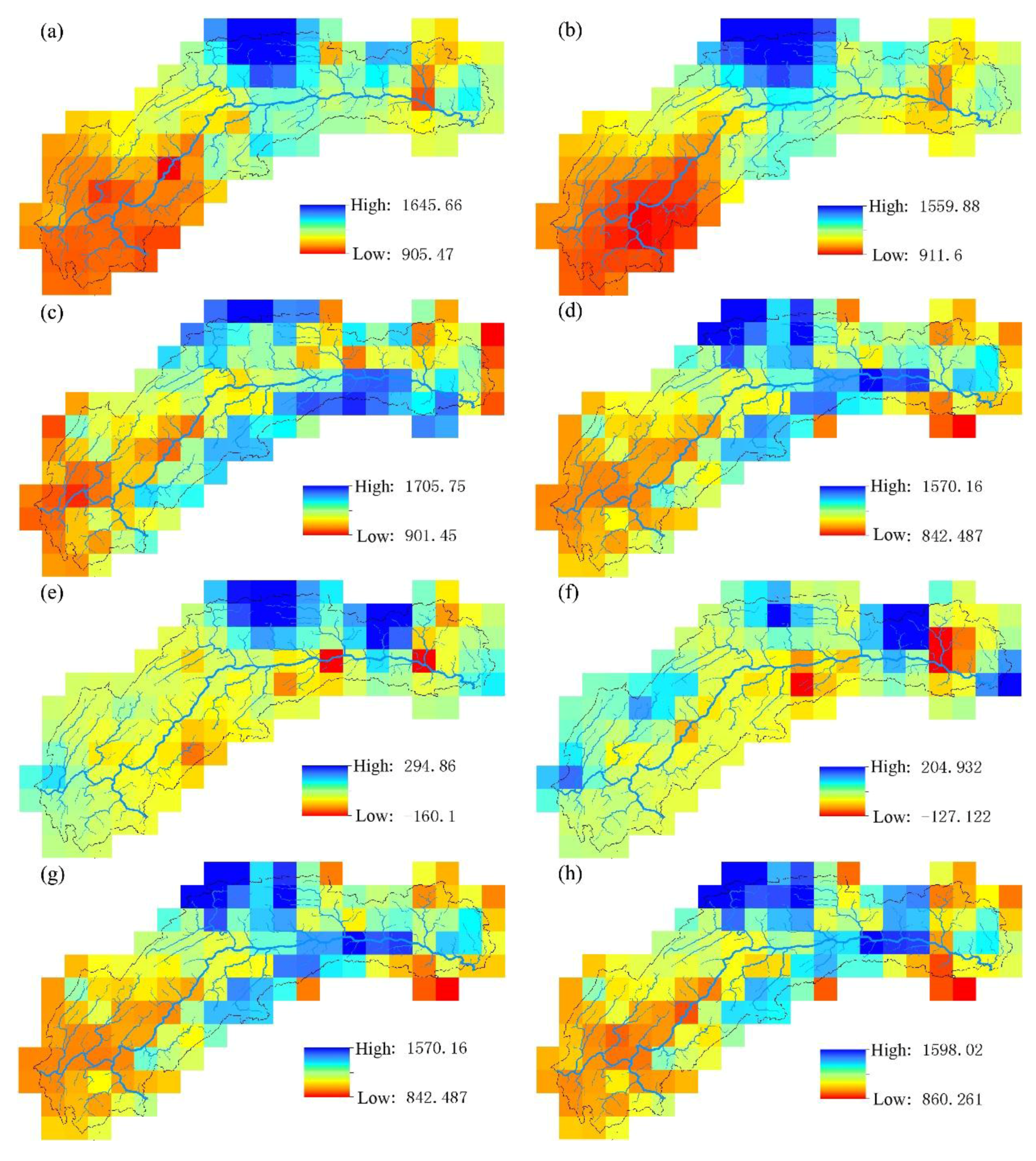
Overall, the distribution of multi-year average annual precipitation in the Three Gorges Region varied greatly, and the low elevation area above the west section of Fengjie has less precipitation; while the canyon alpine area below the eastern section of Fengjie has more precipitation; and the rainy center is located in the Yanshui area.
Comparison of auxiliary variables: Taking the influence factors of precipitation such as longitude, latitude, slope, exposure and elevation of sites into account, this study chose latitude and elevation as auxiliary variables of precipitation interpolation in accordance with related analysis results shown in Table 1. Precipitation data offered by the TRMM satellite could reflect characteristics of the spatial distribution of precipitation, so they were also included as auxiliary variables. We selected four combinations of auxiliary variables and multi-year average annual precipitation of ground stations to establish a linear regression equation and six combinations to establish an SVM model. Due to the representativeness and independence of characteristic information, each combination should have no more than three auxiliary variables of different types. The predictive results of the linear regression equation (from the fifteenth to the eighteenth line in Table 3) show that the E-Tfs and E10-Tfs combined interpolation accuracy with satellite precipitation data is significantly higher than that of the Y-E and E10 without satellite precipitation data. The predictive results of the SVM model (from the first to the sixth line in Table 3) show that the SVM model based on latitude and elevation information only (Y-E, Y-E10) has poor interpolation accuracy, while adding the satellite precipitation data as the auxiliary variable greatly improves the interpolation accuracy, and the three combinations of Y-E-T, Y-E-Tfs and Y-E10-T obtain better interpolation results than the inverse distance weighting and ordinary kriging method. The terrain of the Three Gorges Region is complex and varied, and the precipitation is obviously affected by latitude and elevation. However, using only the latitude, elevation information and precipitation to establish a linear regression equation or SVM model cannot provide high interpolation accuracy. The TRMM satellite precipitation data, despite a certain deviation, has good spatial distribution continuity and better reflects the basin precipitation trend. It provides an effective supplement to the latitude and elevation information, so adding the satellite precipitation data as auxiliary information makes the interpolation effect better.
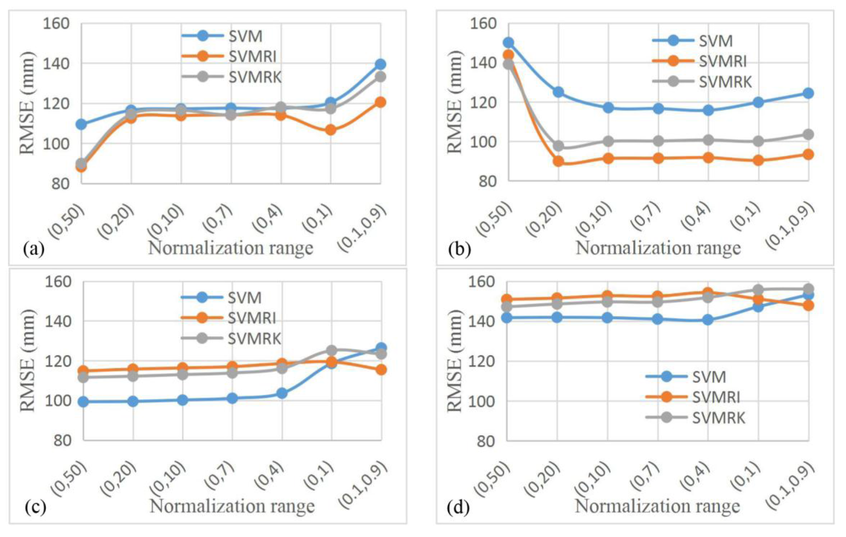
Comparison of the normalized range of the SVM model: Each input variable has a different dimension and range from the target value. For example, the site latitude only changes by 2.3°, and the maximum elevation range within 10 km of the station changes 2259 m. Normalization of input variables and target data can prevent the variables of a large dynamic range from drowning the variables of a small dynamic range, making them have the same effect. The data normalization range has a great influence on the prediction accuracy of the SVM model. In this study, we selected seven normalization ranges of (0, 50), (0, 20), (0, 10), (0, 7), (0, 4), (0, 1), (0.1, 0.9) for comparison. The best and worst normalization ranges of the RMSE value in the SVM model are shown in Table 4. It can be seen from Figure 10 that the SVM model is more stable when the normalization range is (0, 10), (0, 7) and (0, 4). When the normalization range is (0, 50), (0, 20), (0, 1) and (0.1, 0.9), the SVM model is more sensitive, and the probability of extreme values increases. Based on the results of 14 sets, the best RMSE has the highest probability to appear at (0, 50), reaching 50%; the worst RMSE has the highest probability to appear at (0.1, 0.9), reaching 42.86%. Therefore, using the experiment to select a suitable normalization range helps the model achieve better predictive results.
Comparison of the linear regression hybrid interpolation method and the SVM hybrid interpolation method: As shown in Table 3, hybrid interpolation methods show the highest precision where their precipitation estimations are close to the actual results. This is mainly because, by hybrid interpolation methods, the supplementary information of precipitation, including geographical positions, topographic features and satellite precipitation data of a spatially-continuous distribution, was considered comprehensively. In addition, linear regression equation and SVM residuals were further modified through inverse distance weighting and ordinary kriging interpolation methods, improving the interpolation accuracy of the linear regression equation and SVM. Table 5 shows that, after the regression residuals and the SVM residuals are respectively interpolated, the reduction degree of linear regression interpolation RMSE is significantly higher than that of SVM RMSE. To explain this, first, the SVM model overall has better direct predictive results than the linear regression equation; thus, it has less room for improvement. Second, the linear regression equation is simpler and more stable than the SVM. The regression residuals retain more precipitation feature information than the SVM residuals. Although the linear regression hybrid interpolation method has a stronger residual correcting effect than the SVM hybrid interpolation method, the SVM hybrid interpolation method obtains better interpolation results than the linear regression hybrid interpolation method, because the linear regression equation posits a linear relationship between the interpolated object and auxiliary variable, while the SVM model better fits the complex nonlinear relationship between the interpolated object and auxiliary variable.
The SVM model Y-E-T and Y-E-Tfs combined RMSE value is about 120 mm (from the second to the third line in Table 3), and as shown in Figure 10a,b, after correcting the residuals, the interpolation accuracy improves to a certain degree. The SVM model Y-E10-T combined RMSE value is about 100 mm (from the fifth line in Table 3); the Y-E-Tfs combined RMSE value is about 140 mm (from the sixth line in Table 3); as shown in Figure 10c,d, the interpolation precision is reduced to a certain degree after the residuals are corrected. However, when the normalization range is (0.1, 0.9), while there is a decrease of the SVM model fitting accuracy, the SVM hybrid interpolation method has a certain degree of improvement in interpolation accuracy. In this study, we believe that, whether the SVM hybrid interpolation method can further improve the SVM model interpolation accuracy to a certain extent depends on the SVM model fitting accuracy. Choosing a suitable fitting accuracy, though difficult, is the key to ensuring the prediction accuracy of the SVM hybrid interpolation method.
Comparison of single station prediction results (Figure 7 and Figure 8) showed that the regression hybrid interpolation method better predicted the precipitation of the Yanshui, Hexing, Tangfang and Xunleping stations than the multi-element linear regression method. The support vector machine hybrid interpolation method better predicted the precipitation of the Xunleping station than the SVM. However, the regression hybrid interpolation method and the SVM hybrid interpolation method failed to successfully predict the precipitation of Shuiyuesi station, for two reasons. First, the Shuiyuesi station is located in the area where there are too few rainfall stations. Second, the TRMM data have a certain degree of deviation, whose overall effect makes the station precipitation forecast results significantly larger. He et al. (2005) pointed out that the most significant variation of the regional precipitation interpolation comes from the number of meteorological stations and the spatial interpolation method [1]. The establishment of the regional precipitation and auxiliary variables’ linear regression equation and the SVM can minimize the dependence of the interpolation method on the density of meteorological stations, but it still requires a basic number of stations.
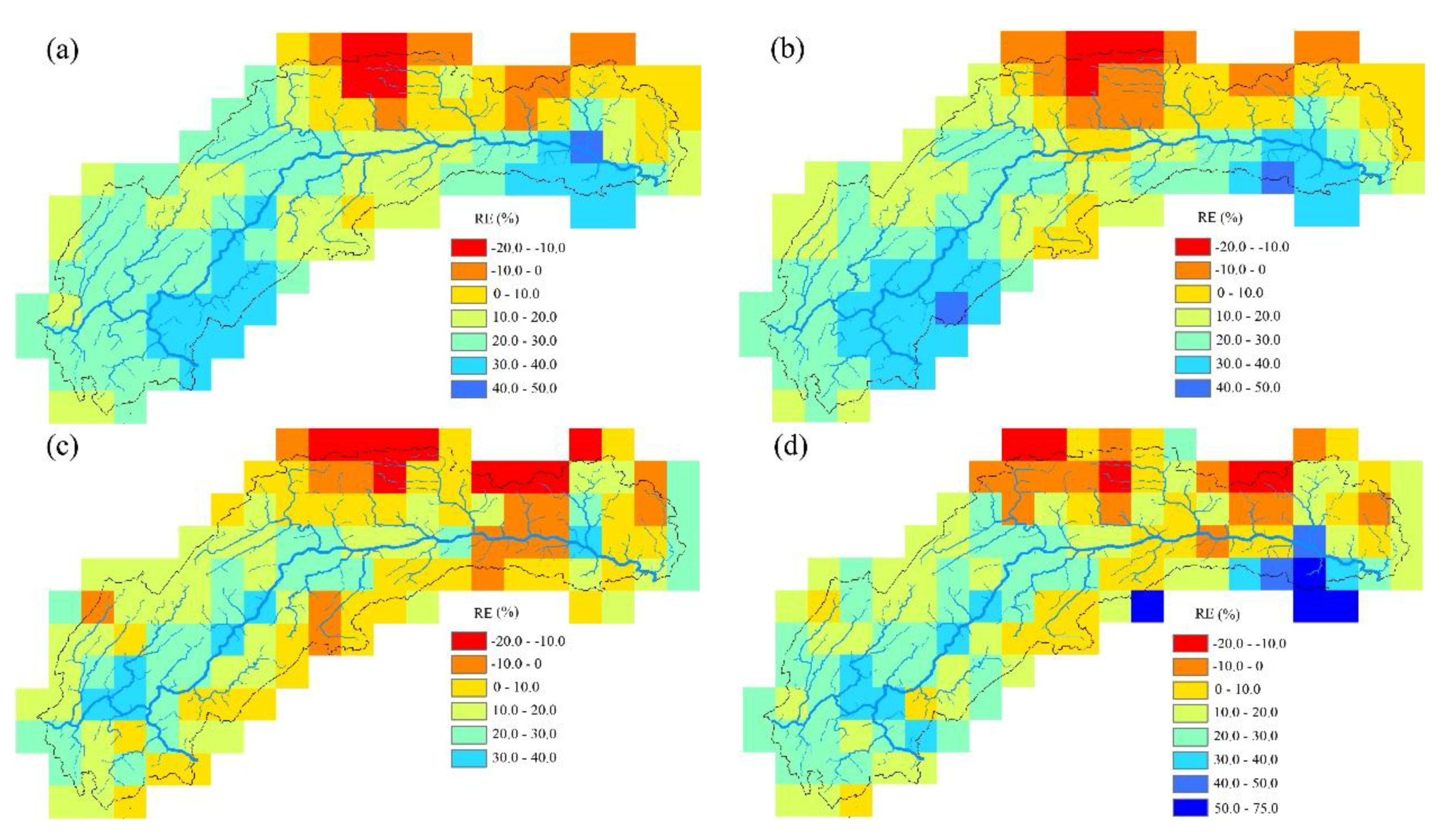
The interpolation results of ground site precipitation and TRMM satellite data were compared: the average precipitation (127 grids, 0.25° × 0.25°) of the Three Gorges Region was calculated by using the four interpolation methods of IDW, OK, LRI and SVMRI. Using the interpolated precipitation, we calculated the relative error of the corresponding TRMM data (Table 6). The distribution of grid relative error is shown in Figure 11.
Figure 11 shows that the TRMM data relative error is negative at the rainy center of the basin, while other areas are basically positive. Table 6 shows that the basin multi-year average annual precipitation calculated by the TRMM data and LRI interpolation has the least relative error, and the SVMRI relative error is slightly smaller than the IDW and OK. This is because the LRI and SVMRI use the TRMM data as the auxiliary variable in the interpolation process, such that the TRMM data have a certain degree of contribution to the final interpolation results. However, the linear regression equation has a greater degree of dependency on the TRMM data than the SVM. The SVM accepts the TRMM data information while maintaining its independence, taking into account that the TRMM data linear regression and the linear regression hybrid interpolation method are not suitable for evaluating TRMM data.
4.2. Discussion
On the whole, using the SVM model and the hybrid interpolation method based on the SVM can produce better precipitation simulation and predictive results, but one needs to solve the following problems in the application of the model:
- The insensitive loss parameter , normalization range and other parameters of the SVM model have an impact on the final interpolation results. Rainfall has strong spatiotemporal distribution characteristics, and the rainfall in each region and at each time is not exactly the same, so it is necessary to adjust the parameters according to each set of data. The workload is large and restricted by personal experience and judgment, and the universality of the SVM model needs to be further strengthened.
- The SVM model can well fit the complex nonlinear relationship between the interpolation object and auxiliary variable. After the residual interpolation is superimposed, the prediction accuracy may be improved, or may be reduced, depending on the fitting degree of the SVM model. Choosing a suitable fitting accuracy so that the residuals retain enough precipitation feature information is the key to improving the prediction accuracy of the SVM hybrid interpolation method, but also its chief difficulty.
- Research data were divided into training samples and test samples randomly. During the training phase, SVM could reach the highest forecast accuracy by cross-validation; and in the test phase, the overall error indicator of test samples was used to verify models. Although test samples are random, the verification needs to be richer and more representative. Spatial interpolation calculation of precipitation with multiple time scales and different spatial scopes will result in more scientific and rational conclusions.
In addition, the satellite precipitation data are evenly distributed in the basin and, thus, can effectively characterize the spatial distribution of precipitation in the basin. The study results show that taking satellite precipitation data as auxiliary variables can greatly enhance the interpolation precision of measured precipitation on sites, which is inconsistent with research findings by Oke et al. (2009), Álvarez-Villa et al. (2011), Wagner et al. (2012) and Teng et al. (2014) [26,27,28,29]. However, the satellite precipitation data already have some deviation. Li and Shao (2010), Sun et al. (2014) and Pan et al. (2015) calibrated the precision of satellite precipitation data by multiple methods [36,37,38]. If calibrated satellite precipitation data are used as auxiliary variables, the interpolation precision of measured precipitation on sites will be further improved.
5. Conclusions
We selected a total of three categories and five types of auxiliary variables including the site latitude, elevation, maximum elevation within 10 km of the site, TRMM multi-year average annual precipitation and flood season precipitation; conducted spatial interpolation of the multi-year average annual precipitation of the ground stations in the Three Gorges Region; established the SVM, the SVM residual inverse distance weighting and the SVM residual kriging precipitation spatial interpolation model; and compared with linear regression and the linear regression hybrid interpolation method, the inverse distance weighting method and the ordinary kriging method. Our results are as follows.
- TRMM 3B43 V7 data deviate from ground site precipitation. Overall, the value is too large, and the rainy center is too small. TRMM data detect the basin precipitation-rich center locations relatively accurately, showing a good spatial distribution continuity, to make up for the shortcomings that the number of local ground sites is insufficient or the distribution is unfavorable. When only the latitude, elevation information and precipitation are used to establish the linear regression equation, the SVM model has poor interpolation precision. Adding the satellite precipitation data as an auxiliary variable significantly improves the interpolation accuracy.
- The support vector machine and SVM hybrid interpolation method obtain better interpolation results than the inverse weight method and ordinary kriging method. The direct predictive result of the SVM model is overall better than that of the linear regression equation. The SVM hybrid interpolation method also obtains better interpolation results than the linear regression hybrid interpolation method.
- The SVM hybrid interpolation method depends on the SVM fitting degree, but it is not the case that the better SVM fits, the higher accuracy the SVM hybrid interpolation method has. The difficult task of choosing a suitable accuracy is the key to improving the prediction accuracy of the SVM.
- The linear regression equation has a greater degree of dependence on the TRMM data than the SVM. The SVM accepts the TRMM data information while maintaining its independence, taking into account that TRMM data linear regression and linear regression hybrid interpolation methods are not suitable for TRMM data evaluation.
Targeting different regions or different time scales of rainfall, the interpolation methods based on different principles also show different interpolation accuracies. For a large number of spatial interpolation methods, there is no absolute optimal method, only the optimal method under specific conditions [39]. In addition to the current widely-used IDW, OK and other methods, SVMs can also be used as an interpolation option. The SVM model can describe the complex nonlinear relationship between the auxiliary variables such as geometric location, terrain feature, satellite precipitation and ground station precipitation and has a good predictive effect. The hybrid interpolation method based on the SVM can further improve the interpolation accuracy and can be studied and applied in the field of rainfall spatial interpolation.
Acknowledgments
Research leading to this paper was supported by Sichuan Science and Technology Support Program, Project 2015SZ0212. Thanks go to the Three Gorges Water Conservancy Complex Cascade Dispatch & Communication Center for providing the research data.
Author Contributions
Xiaoxiao Zhang and Guodong Liu came up with the idea and study; Xiaoxiao Zhang performed the analyses and wrote the paper; Guodong Liu modified the manuscript; Hantao Wang and Xiaodong Li helped in collecting the data.
Conflicts of Interest
The authors declare no conflict of interest.
References
- Zhang, J.G.; Xie, P.; Gong, Y.B.; Liu, G.F. Review and perspectives of the research on spatial interpolation of rainfall information. J. Water Res. Water Eng. 2012, 23, 6–9. (In Chinese) [Google Scholar]
- He, H.Y.; Guo, Z.H.; Xiao, W.F. Review on spatial interpolation techniques of rainfall. Chin. J. Ecol. 2005, 24, 1187–1191. (In Chinese) [Google Scholar]
- Li, J.; Heap, A.D. Spatial interpolation methods applied in the environmental sciences: A review. Environ. Model. Softw. 2014, 53, 173–189. [Google Scholar] [CrossRef]
- Lin, J.Y.; Cheng, C.T.; Chau, K.W. Using support vector machines for long-term discharge prediction. Hydrol. Sci. J. 2006, 51, 599–612. [Google Scholar] [CrossRef]
- Asefa, T.; Kemblowski, M.; Mckee, M.; Khalil, A. Multi-time scale stream flow predictions: The support vector machines approach. J. Hydrol. 2006, 318, 7–16. [Google Scholar] [CrossRef]
- Granata, F.; Gargano, R.; de Marinis, G. Support vector regression for rainfall-runoff modeling in urban drainage: A comparison with the EPA’s storm water management model. Water 2016, 8, 69. [Google Scholar] [CrossRef]
- Langhammer, J.; Česák, J. Applicability of a nu-support vector regression model for the completion of missing data in hydrological time series. Water 2016, 8, 560. [Google Scholar] [CrossRef]
- Tripathi, S.; Srinivas, V.V.; Nanjundiah, R.S. Downscaling of precipitation for climate change scenarios: A support vector machine approach. J. Hydrol. 2006, 330, 621–640. [Google Scholar] [CrossRef]
- Chen, S.T.; Yu, P.S.; Tang, Y.H. Statistical downscaling of daily precipitation using support vector machines and multivariate analysis. J. Hydrol. 2010, 385, 13–22. [Google Scholar] [CrossRef]
- Granata, F.; Papirio, S.; Esposito, G.; Gargano, R.; de Marinis, G. Machine learning algorithms for the forecasting of wastewater quality indicators. Water 2017, 9, 105. [Google Scholar] [CrossRef]
- Huang, Z.S.; Wang, H.Z.; Zhang, R. An improved kriging interpolation technique based on SVM and its recovery experiment in oceanic missing data. Am. J. Comput. Math. 2012, 2, 56–60. [Google Scholar] [CrossRef]
- Gilardi, N.; Bengio, S. Comparison of four machine learning algorithms for spatial data analysis. Conf. Signals Syst. Comput. 2009, 17, 160–167. [Google Scholar]
- Li, C.P.; Zheng, Y.X.; Li, Z.X.; Zhao, Y.Q. Modeling and Application of Ore Grade Interpolation Based on SVM. In Proceedings of the 2011 Eighth International Conference on Fuzzy Systems and Knowledge Discovery (FSKD), Shanghai, China, 26–28 July 2011; Volume 3, pp. 1522–1525. [Google Scholar]
- Liu, Y.F.; Li, R.X.; Li, C.B.; Liu, X.N. Application of BP neural network and support vector machine to the accumulated temperature interpolation. J. Arid Land Resour. Environ. 2014, 28, 158–165. (In Chinese) [Google Scholar]
- Feng, Y.M.; Liang, J. Space data fitting based on the support vector machine-SVM. Hydrogr. Surv. Chart. 2009, 29, 31–33. (In Chinese) [Google Scholar]
- Li, J.; Heap, A.D.; Potter, A.; Daniell, J.J. Application of machine learning methods to spatial interpolation of environmental variables. Environ. Model. Softw. 2011, 26, 1647–1659. [Google Scholar] [CrossRef]
- Zhu, L.; Huang, J.F. Comparison of spatial interpolation method for precipitation of mountain areas in county scale. Trans. Chin. Soc. Agric. Eng. 2007, 23, 80–85. (In Chinese) [Google Scholar]
- Sun, W.; Zhu, Y.Q.; Huang, S.L.; Guo, C.X. Mapping the mean annual precipitation of China using local interpolation techniques. Theor. Appl. Climatol. 2015, 119, 171–180. [Google Scholar] [CrossRef]
- Bostan, P.A.; Heuvelink, G.B.M.; Akyurek, S.Z. Comparison of regression and kriging techniques for mapping the average annual precipitation of Turkey. Int. J. Appl. Earth. Obs. 2012, 19, 115–126. [Google Scholar] [CrossRef]
- Seo, Y.; Kim, S.; Singh, V.P. Estimating spatial precipitation using regression kriging and artificial neural network residual kriging (RKNNRK) hybrid approach. Water Resour. Manag. 2015, 29, 2189–2204. [Google Scholar] [CrossRef]
- Kizza, M.; Westerberg, I.; Rodhe, A.; Ntale, H.K. Estimating areal rainfall over Lake Victoria and its basin using ground-based and satellite data. J. Hydrol. 2012, 464, 401–411. [Google Scholar] [CrossRef]
- Tang, G.Q.; Li, Z.; Xue, X.W.; Hu, Q.F.; Yong, B.; Hong, Y. A study of substitutability of TRMM remote sensing precipitation for gauge-based observation in Ganjiang River basin. Adv. Water Sci. 2015, 26, 340–346. (In Chinese) [Google Scholar]
- Tekeli, A.E.; Fouli, H. Evaluation of TRMM satellite-based precipitation indexes for flood forecasting over Riyadh City, Saudi Arabia. J. Hydrol. 2016, 541, 471–479. [Google Scholar] [CrossRef]
- Jiang, S.H.; Zhou, M.; Ren, L.L.; Cheng, X.R.; Zhang, P.J. Evaluation of latest TMPA and CMORPH satellite precipitation products over Yellow River Basin. Water Sci. Eng. 2016, 9, 87–96. [Google Scholar] [CrossRef]
- Yang, Y.C.; Cheng, G.W.; Fan, J.H.; Sun, J.; Li, W.P. Representativeness and reliability of satellite rainfall dataset in alpine and gorge region. Adv. Water Sci. 2013, 24, 24–33. (In Chinese) [Google Scholar]
- Oke, A.M.C.; Frost, A.J.; Beesley, C.A. The use of TRMM satellite data as a predictor in the spatial interpolation of daily precipitation over Australia. In Proceedings of the 18th World IMACS/MODSIM Congress on Modelling and Simulation, Cairns, Australia, 13–17 July 2009; Volume 1, pp. 3726–3732. [Google Scholar]
- Álvarez-Villa, O.D.; Vélez, J.I.; Poveda, G. Improved long-term mean annual rainfall fields for Colombia. Int. J. Climatol. 2011, 31, 2194–2212. [Google Scholar] [CrossRef]
- Wagner, P.D.; Fiener, P.; Wilken, F.; Kumar, S.; Schneider, K. Comparison and evaluation of spatial interpolation schemes for daily rainfall in data scarce regions. J. Hydrol. 2012, 464, 388–400. [Google Scholar] [CrossRef]
- Teng, H.F.; Shi, Z.; Ma, Z.Q.; Li, Y. Estimating spatially downscaled rainfall by regression kriging using TRMM precipitation and elevation in Zhejiang Province, southeast China. Int. J. Remote Sens. 2014, 35, 7775–7794. [Google Scholar] [CrossRef]
- Li, Z. Multi-source Precipitation Observations and Fusion for Hydrological Applications in the Yangtze River Basin. Ph.D. Thesis, Tsinghua University, Beijing, China, 2015. (In Chinese). [Google Scholar]
- Hu, Q.F.; Yang, D.W.; Wang, Y.T.; Yang, H.B. Monthly runoff simulation in Gan river basin using rainfall TRMM 3B43V7. J. Hydroelectr. Eng. 2014, 33, 6–12. (In Chinese) [Google Scholar]
- Tang, G.A.; Yang, X. ArcGIS Geographic Information System Spatial Analysis the Experimental Tutorial (2); Science Press: Beijing, China, 2012. (In Chinese) [Google Scholar]
- Ly, S.; Charles, C.; Degré, A. Different methods for spatial interpolation of rainfall data for operational hydrology and hydrological modeling at watershed scale: A review. Biotechnol. Agron. Soc. Environ. 2013, 17, 392–406. [Google Scholar]
- Vicente-Serrano, S.M.; Saz-Sánchez, M.A.; Cuadrat, J.M. Comparative analysis of interpolation methods in the middle Ebro Valley (Spain): Application to annual precipitation and temperature. Clim. Res. 2003, 24, 161–180. [Google Scholar] [CrossRef]
- Wang, X.C.; Shi, F.; Yu, L.; Li, Y. MATLAB Neural Network Analysis of 43 Cases; Beihang University Press: Beijing, China, 2016. (In Chinese) [Google Scholar]
- Li, M.; Shao, Q.X. An improved statistical approach to merge satellite rainfall estimates and raingauge data. J. Hydrol. 2010, 385, 51–64. [Google Scholar] [CrossRef]
- Sun, L.Q.; Hao, Z.C.; Wang, J.H.; Nistor, I.; Seidou, O. Assessment and correction of TMPA products 3B42RT and 3B42V6. J. Hydraul. Eng. 2014, 46, 1135–1146. (In Chinese) [Google Scholar]
- Pan, Y.; Shen, Y.; Yu, J.J.; Xiong, A.Y. An experiment of high-resolution gauge-radar-satellite combined precipitation retrieval based on the Bayesian merging method. Acta Meteorol. Sin. 2015, 73, 177–186. (In Chinese) [Google Scholar]
- Li, X.; Cheng, G.D.; Lu, L. Comparison of spatial interpolation methods. Adv. Earth Sci. 2000, 15, 260–265. (In Chinese) [Google Scholar]
Figure 1.
Spatial distribution of rainfall sites in study area.

Figure 2.
TRMM satellite data in the study area ((a) TRMM multi-year average annual precipitation; (b) TRMM multi-year average flood season precipitation).
Figure 2.
TRMM satellite data in the study area ((a) TRMM multi-year average annual precipitation; (b) TRMM multi-year average flood season precipitation).

Figure 3.
Time series correlation coefficient ((a) annual precipitation; (b) flood season precipitation).
Figure 3.
Time series correlation coefficient ((a) annual precipitation; (b) flood season precipitation).

Figure 4.
Precipitation relative errors ((a) multi-year average annual precipitation; (b) multi-year average flood season precipitation).
Figure 4.
Precipitation relative errors ((a) multi-year average annual precipitation; (b) multi-year average flood season precipitation).

Figure 5.
Structure of the nonlinear support vector machine.

Figure 6.
Flowchart of the support vector machine residual hybrid interpolation method.

Figure 7.
Test station multi-year average annual precipitation ((a) linear regression and its hybrid interpolation method; (b) support vector machine and its hybrid interpolation method).
Figure 7.
Test station multi-year average annual precipitation ((a) linear regression and its hybrid interpolation method; (b) support vector machine and its hybrid interpolation method).

Figure 8.
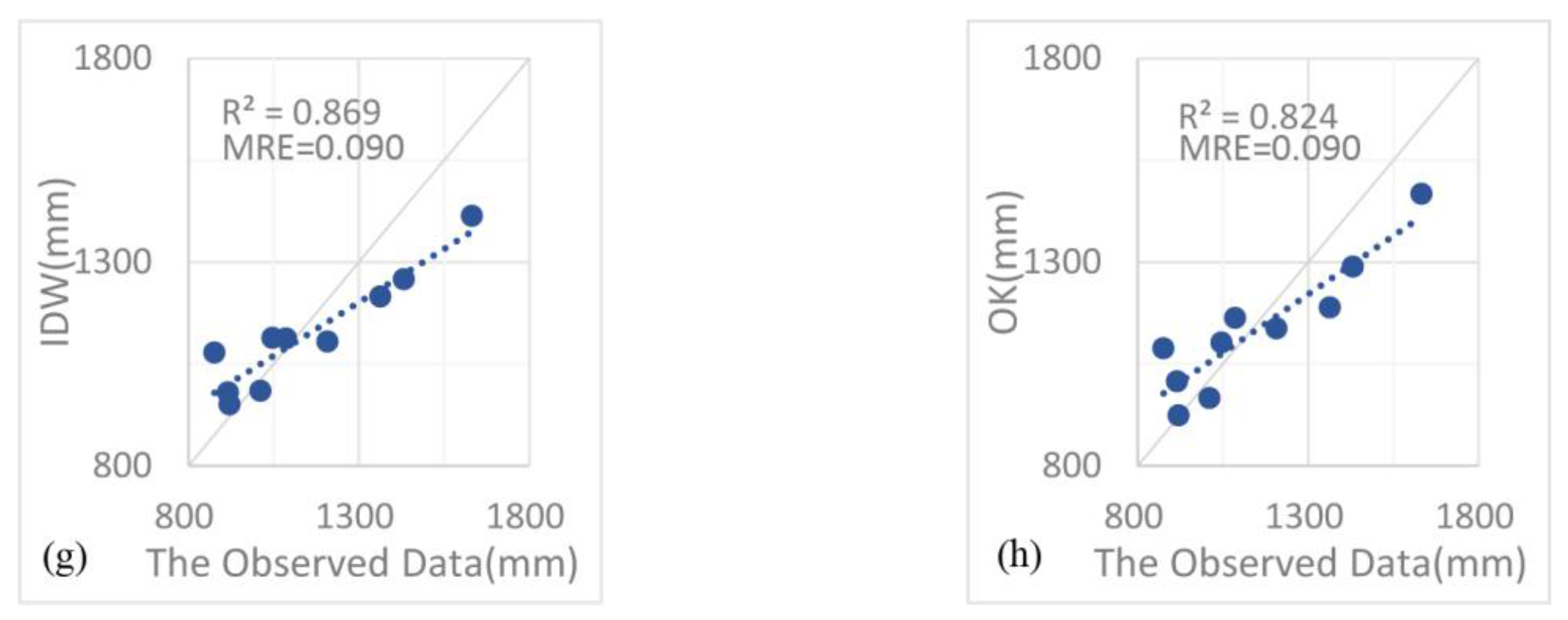
Scatter diagrams of test station multi-year average annual precipitation ((a) SVM; (b) SVMRI; (c) SVMRK; (d) LR; (e) LRI; (f) LRK; (g) IDW; (h) OK).
Figure 8.
Scatter diagrams of test station multi-year average annual precipitation ((a) SVM; (b) SVMRI; (c) SVMRK; (d) LR; (e) LRI; (f) LRK; (g) IDW; (h) OK).


Figure 9.
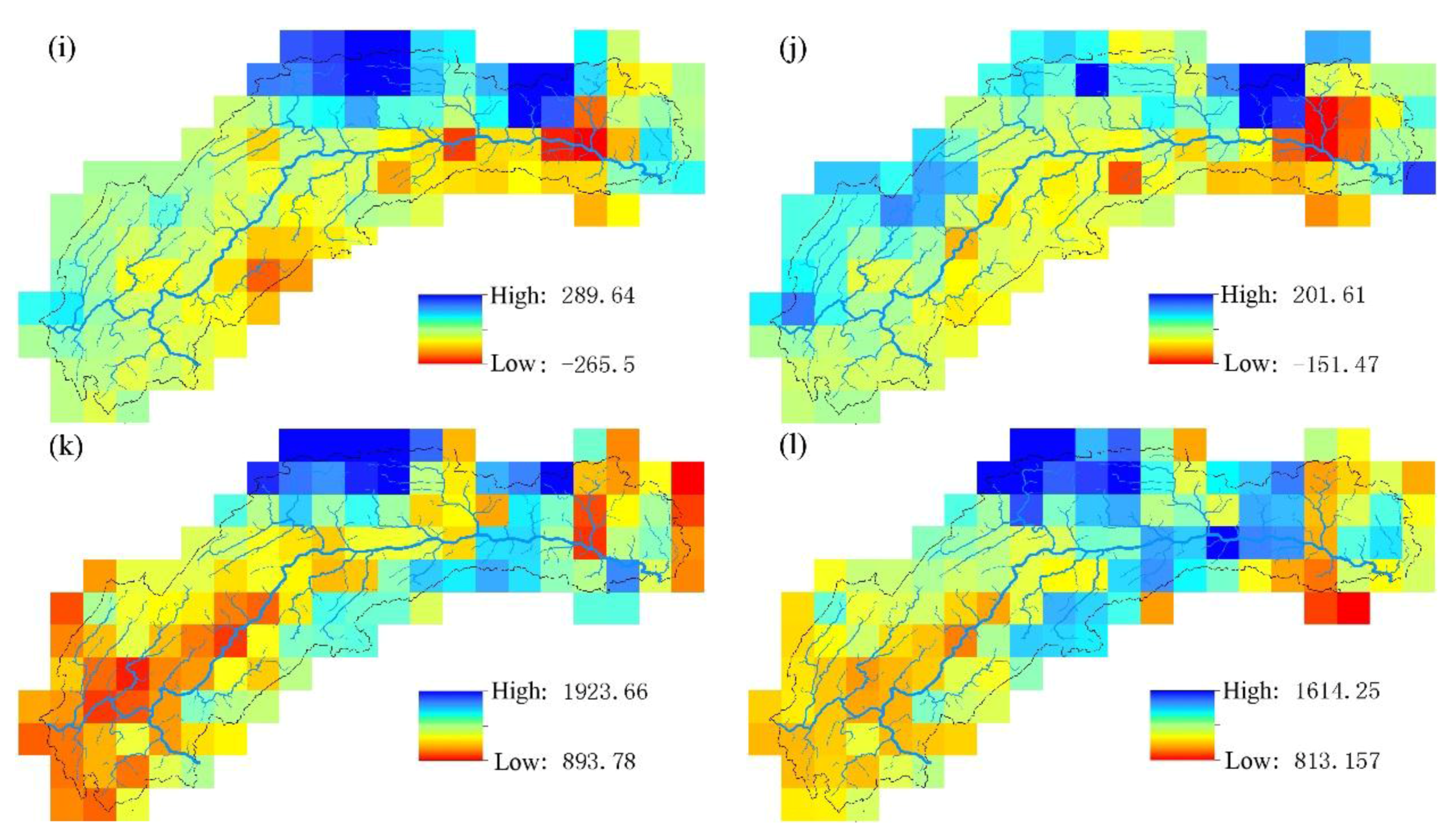
Multi-year average annual precipitation interpolation results in the Three Gorges Region ((a) IDW; (b) OK; (c) LR; (d) SVM; (e) LRRE-IDW; (f) SVMRE-IDW; (g) LRI; (h) SVMRI; (i) LRRE-OK; (j) SVMRE-OK; (k) LRK; (l) SVMRK).
Figure 9.
Multi-year average annual precipitation interpolation results in the Three Gorges Region ((a) IDW; (b) OK; (c) LR; (d) SVM; (e) LRRE-IDW; (f) SVMRE-IDW; (g) LRI; (h) SVMRI; (i) LRRE-OK; (j) SVMRE-OK; (k) LRK; (l) SVMRK).


Figure 10.
Comparison of normalization ranges ((a) Y-E-T; (b) Y-E-Tfs; (c) Y-E10-T; (d) Y-E10-Tfs).

Figure 11.
Grid relative errors ((a) IDW; (b) OK; (c) LRI; (d) SVMRI).


Table 1.
Correlation coefficient between the precipitation of 41 stations and each auxiliary variable.
Table 1.
Correlation coefficient between the precipitation of 41 stations and each auxiliary variable.
| Correlation Coefficient | Geographic Location | Terrain Characteristics | Satellite Precipitation | |||||
|---|---|---|---|---|---|---|---|---|
| X | Y | S | A | E | E10 | T | Tfs | |
| Pearson | 0.226 | 0.540 ** | 0.275 | 0.198 | 0.567 ** | 0.610 ** | 0.387 * | 0.528 ** |
| Spearman | 0.338 * | 0.536 ** | 0.271 | 0.383 * | 0.524 ** | 0.552 ** | 0.453 ** | 0.497 ** |
Note: * Significant correlation at the 0.05 level (bilateral); ** significant correlation at the 0.01 level (bilateral).
Table 2.
Regression equations at a glance.
| Dependent Variable | Initial Independent Variable | Independent Variable Removed (Not Significant) | Final Independent Variable (Significant) | Regression Equation (Significant) | |
|---|---|---|---|---|---|
| P | 1 | Y-E-T | T | Y-E | P = −2819.38 + 123.69 × Y + 0.24 × E |
| 2 | Y-E-Tfs | Y | E-Tfs | P = −288.08 + 0.27 × E + 1.39 × Tfs | |
| 3 | Y-E10-T | Y, T | E10 | P = 791.61 + 0.20 × Z10 | |
| 4 | Y-E10-Tfs | Y | E10-Tfs | P = −539.24 + 0.19 × Z10 + 1.40 × Tfs | |
Table 3.
Test station error indicators. SVMRI, SVM residual inverse distance weighting; SVMRK, SVM residual kriging; LRI, linear regression residual inverse distance weighting; LRK, linear regression residual kriging.
Table 3.
Test station error indicators. SVMRI, SVM residual inverse distance weighting; SVMRK, SVM residual kriging; LRI, linear regression residual inverse distance weighting; LRK, linear regression residual kriging.
| Method | Test Set RMSE (mm) | Test Set MRE | Test Set R2 | |||||||
|---|---|---|---|---|---|---|---|---|---|---|
| Worst | Mean | Best | Worst | Mean | Best | Worst | Mean | Best | ||
| SVM | Y-E | 262.596 | 252.111 | 231.954 | 0.158 | 0.155 | 0.152 | 0.236 | 0.238 | 0.226 |
| Y-E-T | 139.397 | 119.676 | 109.445 | 0.097 | 0.078 | 0.073 | 0.735 | 0.767 | 0.793 | |
| Y-E-Tfs | 150.120 | 124.128 | 115.792 | 0.110 | 0.086 | 0.079 | 0.633 | 0.746 | 0.770 | |
| Y-E10 | 230.890 | 222.975 | 203.216 | 0.127 | 0.127 | 0.125 | 0.427 | 0.439 | 0.459 | |
| Y-E10-T | 126.379 | 106.926 | 99.289 | 0.089 | 0.072 | 0.068 | 0.757 | 0.811 | 0.831 | |
| Y-E10-Tfs | 153.183 | 143.917 | 140.692 | 0.109 | 0.088 | 0.085 | 0.613 | 0.674 | 0.693 | |
| SVMRI | Y-E-T | 120.502 | 109.988 | 88.255 | 0.092 | 0.079 | 0.066 | 0.801 | 0.830 | 0.883 |
| Y-E-Tfs | 143.777 | 98.873 | 89.958 | 0.106 | 0.076 | 0.071 | 0.673 | 0.835 | 0.865 | |
| Y-E10-T | 119.379 | 116.727 | 114.794 | 0.085 | 0.082 | 0.081 | 0.761 | 0.769 | 0.773 | |
| Y-E10-Tfs | 154.225 | 151.522 | 147.850 | 0.098 | 0.096 | 0.099 | 0.610 | 0.623 | 0.656 | |
| SVMRK | Y-E-T | 133.255 | 114.803 | 89.902 | 0.108 | 0.086 | 0.070 | 0.766 | 0.809 | 0.874 |
| Y-E-Tfs | 139.153 | 105.924 | 97.733 | 0.103 | 0.082 | 0.077 | 0.704 | 0.811 | 0.838 | |
| Y-E10-T | 125.083 | 116.418 | 111.540 | 0.089 | 0.083 | 0.081 | 0.739 | 0.769 | 0.785 | |
| Y-E10-Tfs | 156.121 | 151.206 | 147.150 | 0.105 | 0.095 | 0.088 | 0.626 | 0.631 | 0.645 | |
| L | Y-E | 170.976 | 0.106 | 0.504 | ||||||
| E-Tfs | 145.495 | 0.108 | 0.681 | |||||||
| E10 | 191.842 | 0.116 | 0.488 | |||||||
| E10-Tfs | 145.771 | 0.092 | 0.775 | |||||||
| LRI | Y-E | 108.666 | 0.081 | 0.816 | ||||||
| E-Tfs | 90.303 | 0.071 | 0.868 | |||||||
| E10 | 144.099 | 0.098 | 0.719 | |||||||
| E10-Tfs | 128.143 | 0.085 | 0.768 | |||||||
| LRK | Y-E | 111.001 | 0.087 | 0.796 | ||||||
| E-Tfs | 90.987 | 0.072 | 0.864 | |||||||
| E10 | 147.082 | 0.097 | 0.661 | |||||||
| E10-Tfs | 138.954 | 0.098 | 0.729 | |||||||
| IDW | 127.092 | 0.090 | 0.869 | |||||||
| OK | 121.424 | 0.090 | 0.824 | |||||||
Table 4.
Support vector machine normalization range.
| Input Vector | SVM Normalization Range | SVMRI Normalization Range | SVMRK Normalization Range | |||
|---|---|---|---|---|---|---|
| The Worst RMSE | The Best RMSE | The Worst RMSE | The Best RMSE | The Worst RMSE | The Best RMSE | |
| Y-E | (0, 50) | (0.1, 0.9) | / | / | / | / |
| Y-E-T | (0.1, 0.9) | (0, 50) | (0.1, 0.9) | (0, 50) | (0.1, 0.9) | (0, 50) |
| Y-E-Tfs | (0, 50) | (0, 4) | (0, 50) | (0, 20) | (0, 50) | (0, 20) |
| Y-E10 | (0, 10) | (0.1, 0.9) | / | / | / | / |
| Y-E10-T | (0.1, 0.9) | (0, 50) | (0, 1) | (0, 50) | (0, 1) | (0, 50) |
| Y-E10-Tfs | (0.1, 0.9) | (0, 4) | (0, 4) | (0.1, 0.9) | (0.1, 0.9) | (0, 50) |
Table 5.
RMSE reduction degree of the hybrid interpolation method.
| Support Vector Machine Hybrid Interpolation | Linear Regression Hybrid Interpolation | ||||
|---|---|---|---|---|---|
| Auxiliary Variable | SVMRI | SVMRK | Auxiliary Variable | LRI | LRK |
| Y-E-T | −19.36% | −17.86% | Y-E | −36.44% | −35.08% |
| Y-E-Tfs | −22.31% | −15.60% | E-Tfs | −35.11% | −37.46% |
| Y-E10-T | 15.62% | 12.34% | E10 | −24.89% | −23.33% |
| Y-E10-Tfs | 5.09% | 4.59% | E10-Tfs | −17.92% | −4.68% |
Table 6.
Basin average precipitation relative error.
| Index | IDW | OK | LRI | SVMRI |
|---|---|---|---|---|
| Gauge precipitation (mm) | 1085.811 | 1094.046 | 1165.304 | 1109.604 |
| TRMM (mm) | 1267.984 | 1267.984 | 1267.984 | 1267.984 |
| Relative error | 16.78% | 15.90% | 8.81% | 14.27% |
© 2017 by the authors. Licensee MDPI, Basel, Switzerland. This article is an open access article distributed under the terms and conditions of the Creative Commons Attribution (CC BY) license (http://creativecommons.org/licenses/by/4.0/).
Share and Cite
MDPI and ACS Style
Zhang, X.; Liu, G.; Wang, H.; Li, X. Application of a Hybrid Interpolation Method Based on Support Vector Machine in the Precipitation Spatial Interpolation of Basins. Water 2017, 9, 760. https://doi.org/10.3390/w9100760
AMA Style
Zhang X, Liu G, Wang H, Li X. Application of a Hybrid Interpolation Method Based on Support Vector Machine in the Precipitation Spatial Interpolation of Basins. Water. 2017; 9(10):760. https://doi.org/10.3390/w9100760
Chicago/Turabian StyleZhang, Xiaoxiao, Guodong Liu, Hantao Wang, and Xiaodong Li. 2017. "Application of a Hybrid Interpolation Method Based on Support Vector Machine in the Precipitation Spatial Interpolation of Basins" Water 9, no. 10: 760. https://doi.org/10.3390/w9100760
Note that from the first issue of 2016, this journal uses article numbers instead of page numbers. See further details here.