Comparative Analysis of ANN and SVM Models Combined with Wavelet Preprocess for Groundwater Depth Prediction

1
School of Engineering, Anhui Agricultural University, Hefei 230036, China
2
Anhui & Huaihe River Institute of Hydraulic Research; Hefei 230088, China
3
Institute of Huai River Water Resources Protection, Bengbu 233001, China
*
Author to whom correspondence should be addressed.
Water 2017, 9(10), 781; https://doi.org/10.3390/w9100781
Submission received: 25 August 2017
/
Revised: 20 September 2017
/
Accepted: 29 September 2017
/
Published: 12 October 2017
(This article belongs to the Special Issue Groundwater Monitoring and Remediation)
Abstract
:Reliable prediction of groundwater depth fluctuations has been an important component in sustainable water resources management. In this study, a data-driven prediction model combining discrete wavelet transform (DWT) preprocess and support vector machine (SVM) was proposed for groundwater depth forecasting. Regular artificial neural networks (ANN), regular SVM, and wavelet preprocessed artificial neural networks (WANN) models were also developed for comparison. These methods were applied to the monthly groundwater depth records over a period of 37 years from ten wells in the Mengcheng County, China. Relative absolute error (RAE), Pearson correlation coefficient (r), root mean square error (RMSE), and Nash-Sutcliffe efficiency (NSE) were adopted for model evaluation. The results indicate that wavelet preprocess extremely improved the training and test performance of ANN and SVM models. The WSVM model provided the most precise and reliable groundwater depth prediction compared with ANN, SVM, and WSVM models. The criterion of RAE, r, RMSE, and NSE values for proposed WSVM model are 0.20, 0.97, 0.18 and 0.94, respectively. Comprehensive comparisons and discussion revealed that wavelet preprocess extremely improves the prediction precision and reliability for both SVM and ANN models. The prediction result of SVM model is superior to ANN model in generalization ability and precision. Nevertheless, the performance of WANN is superior to SVM model, which further validates the power of data preprocess in data-driven prediction models. Finally, the optimal model, WSVM, is discussed by comparing its subseries performances as well as model performance stability, revealing the efficiency and universality of WSVM model in data driven prediction field.
1. Introduction
Groundwater is an important water source in much of the world, especially in arid and semi-arid regions [1,2]. In recent decades, groundwater often has been overexploited, particularly in developing countries. Groundwater depth, the distance from ground surface to water table, can be measured by monitor wells, thus can be directly observed. Groundwater depth fluctuations are influenced by natural and anthropic stresses, which can be an indicator for the integrated water resources management. When groundwater exploitation exceeds recharge, groundwater depth increases as the water table falls; in contrast, groundwater depth decreases when recharge exceeds exploitation and can lead to water-logging. Accurate prediction of groundwater depth fluctuation has been crucial for regional sustainable water resources management.
Physical and data-driven statistical models are two main tools for groundwater depth prediction [3]. The need of large amounts of data on precipitation, groundwater exploitation, soil nature, and human activities such as operation of channels and dams projects is a significant barrier for physical modeling [1,4]. To achieve reliable groundwater depth prediction, data-driven statistical modeling is a useful alternative approach.
Statistical models are mainly developed to explore the “input-output” pattern of long term groundwater depth data series for make future estimates. Input data can be single groundwater historic series or exogenous with broader types of available data [5]. Multi-variable linear regression model (MLR) has been applied in several groundwater level prediction cases [6,7,8]. Since long term historical groundwater depth records can be considered as correlated time series, autoregressive integrated moving average model (ARIMA) has also been used for groundwater fluctuation forecasting [9,10,11]. The advantage of ARIMA is that it can filter extreme values and decrease their interference in prediction accuracy. Linear regression methods are practical and cost-effective. However, linear fitting is not capable to describe many complex groundwater fluctuation problems. Thus, in recent research, linear regression models were usually carried out as a comparative method to highlight better models.
Artificial neural networks (ANNs) are a promising intelligent method that can efficiently capture internal non-linear characteristics of groundwater fluctuations. Over the last decades, ANN has become one of the most widely used algorithms in groundwater level forecasting [12,13,14,15,16,17] and is frequently compared with linear regression. ANNs are more competitive in prediction accuracy for its high efficiency in abstracting non-linear complicated input-output rules [1,6,8]. However, ANN also has limitations. It is quite sensitive to internal parameters, which brings difficulties in model calibration. Although many other intelligent algorithms such as genetic algorithms, particle swarm algorithms and ant colony optimization were integrated into ANN for parameter calibration [18,19,20,21], underfitting and overfitting are difficult to avoid due to improper model structures and parameters.
Support Vector Machine (SVM) is a modern statistical learning theory in data-driven modeling. The uniqueness of SVM is its structural risk minimization (SRM) objective that balancing model’s complexity against its fitting precision, instead of an empirical risk minimum (ERM) used by most intelligent algorithms that focus mostly on fitting accuracy [22]. This model architecture greatly improves model generalization ability compared with ERM based algorithms such as ANN. In recent years, SVM is used for hydrologic predictions such as stream flows [23,24], precipitation [25,26], sediments [27], and groundwater fluctuations. Most researches found that SVM performs more reliable than ANN. Usually, ANN models have lower mean error than SVM in model calibration, but in model test stage, the mean error of SVM is much lower than ANN, indicating SVM models are often superior in generalization ability [28,29].
A problem for intelligent algorithms in hydrology is that most time series are non-stationary, which may lead to poor forecasting ability. For instance, long term groundwater depth process may be influenced by precipitation, evapotranspiration, seasonal cycle, crop yield, and other random issues. Even non-linear intelligent models cannot guarantee precise description of all these features, or such models may become very complicated for it confounds real features and stochastic noise. Therefore, data preprocessing is another important aspect. Preprocessing can be accomplished in various ways. Deleting abnormal points from observed time series can be regarded as preprocess, but it is usually controversial because simply deleting outliers may disrupt randomness in the sample. In ARIMA models, the moving average (MA) is a preprocess method to smoothen time series data [9,10,11]. Fuzzification, the first step in ANFIS model, which disperses determined data to discrete fuzzy scenarios is also a preprocess method [30,31]. In time series analysis, preprocess is accomplished by separating trend components, cyclical components, seasonal components and random components from original time series. Wavelet analysis decomposes the initial process into several sub-series for regulation. It has been used in hydrologic prediction modeling as a preprocess method coupled with other prediction models. Adamowski et al. [6] proposed an ANN prediction model combined with wavelet transform on input data for daily water demands in Montreal, Canada. The hybrid model showed best fitting precision compared with multiple linear regression (MLR), multiple nonlinear regression (MNLR), ARIMA and traditional ANN model. Suryanarayana et al. [32] proposed a wavelet analysis based SVM model for groundwater level prediction, and the result was also better than SVM, ANN and ARIMA models. However, other models combined with wavelet analysis were not discussed in this paper. Rathinasamy et al. [33] compared three hybrid wavelet models: WVC (Wavelet Volterra Coupled model, proposed by Maheswaran R. et al. [34]), WANN WLR, and two regular models: AR and ANN, which was in agreement that hybrid models performed better than regular models. Furthermore, the wavelet based models outperformed significantly with the increase of lead time. Similar results were also indicated by Moosavi et al. in groundwater level prediction using ANN, ANFIS, WANN and WANFIS models [35].
Nourani et al. [36] gave a state-of-the-art review of hybrid wavelet and artificial intelligence (AI) models development in hydrology. 105 papers were summarized, concluding that the dominant application of wavelet based AI models is stream flow forecasting, and the dominant AI method is ANN with a proportion of 90%. Due to the low number of research papers in groundwater and water quality subject, the authors recommended conducting additional research in these fields.
This study explores and compares data-driven prediction models for monthly groundwater depth. Discrete wavelet transforms are used to preprocess original groundwater depth time series. Four models: regular ANN, regular SVM, wavelet preprocessed ANN (WANN) and wavelet preprocessed SVM (WSVM) were developed and applied in parallel under the same time horizon. The ANN based models represent classic intelligent algorithm, while the SVM models are proposed in this paper to explore more efficient prediction for non-stationary data process. Specifically, the performances of ANN based model and SVM based model were comprehensively compared, drawing a conclusion that SVM based model is superior to ANN based model from both theoretical and practical point of view. Thereafter, the effect of wavelet preprocess was analyzed by comparisons between regular models and wavelet preprocessed models, which demonstrated the role of data preprocessing in non-stationary time series prediction. Finally, the best model, WSVM, was discussed with stability analysis.
2. Study Area and Data
Mengcheng County is in the Huai river basin of Anhui province, China (Figure 1). Mengcheng County is home to 1.40 million people, of which 22.5% are urban and 77.5% are rural. The total area of Mengcheng County is 2091 km2, comprising 318 km2 (15%) urban land and 1773 km2 (85%) of agriculture land, so water is of vital importance for this agrarian county.
The Mengcheng County lies in the north-south climate boundary of China. Annual average precipitation is 873 mm. Mengcheng County relies on groundwater. Precipitation can guarantee groundwater recharge in most years, but there remains great gap between precipitation and water use demands in many years. Therefore, groundwater pumping has long been important supplement in Mengcheng County for it is convenient and cheap, meanwhile the supply is reliable and sustainable.
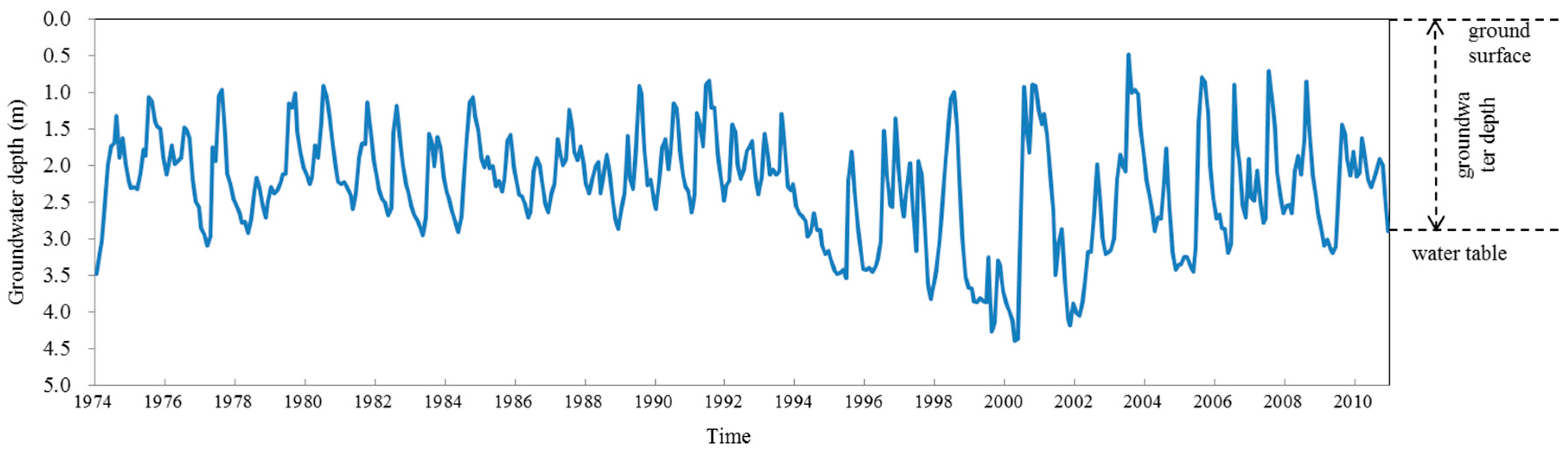
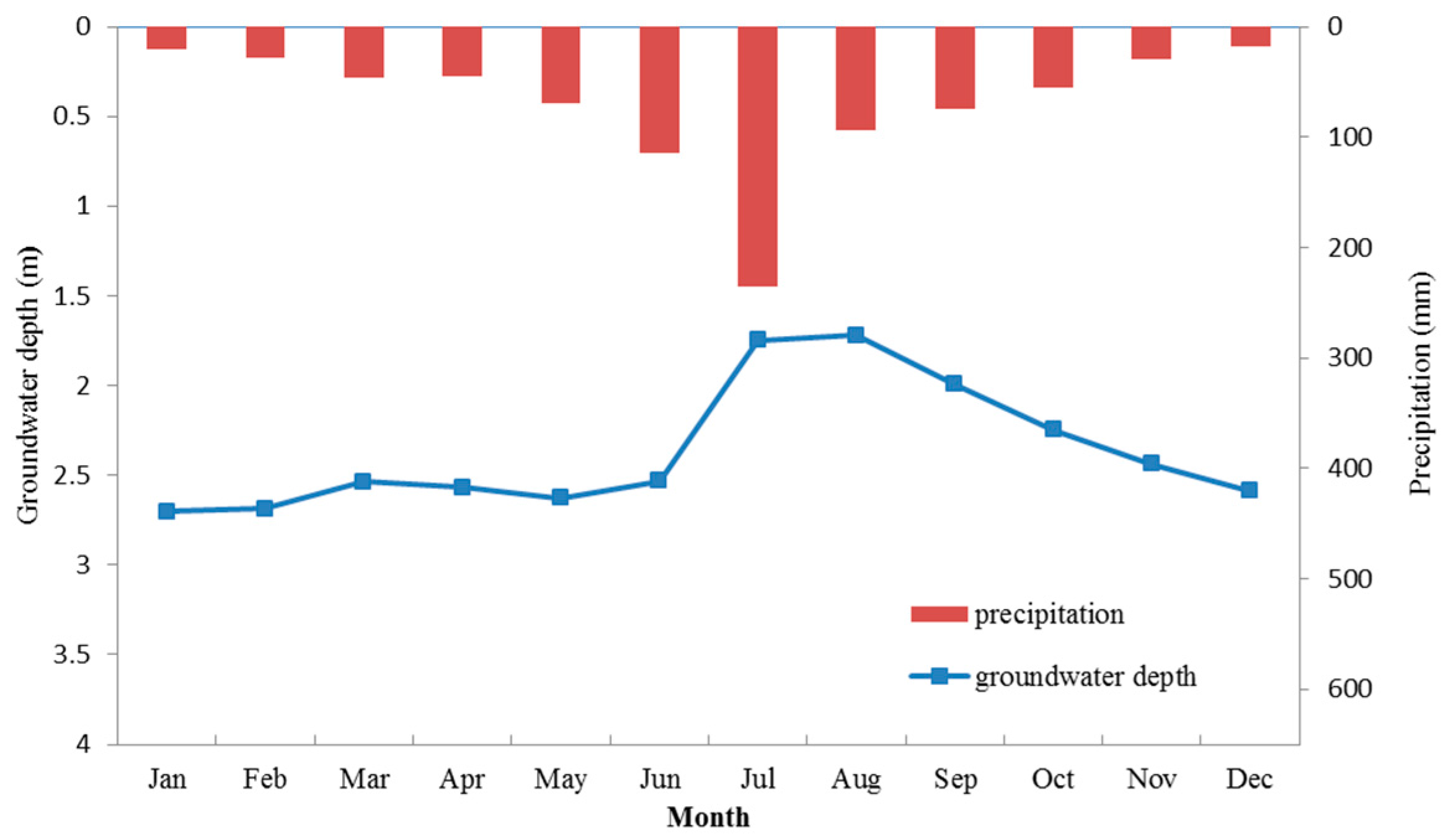
Mengcheng County has been facing severe groundwater depletion, mainly for agriculture. In the 1970s, ten observation wells were set in Mengcheng County to monitor groundwater fluctuations. A total of 444 months were observed with records from January 1974 to December 2010. The well specifications are shown in Table 1. Here we use the average data of the ten wells to represent the groundwater depth fluctuation. Moreover, the averaged monthly groundwater depth series, average groundwater depth and precipitation by month, as well as annual average groundwater depth are shown in Figure 2, Figure 3 and Figure 4, respectively. Several temporal characteristics can be found as follows:
First, the groundwater depth shows seasonal periodicity. Precipitation in Mengcheng County concentrates in June, July and August (Figure 3). Correspondingly, groundwater depth decreases during the three months as the water table rises. In contrast, groundwater depth increases with the decrease of precipitation after September. May and June are exceptions where precipitation increases but groundwater depth does not significantly decrease, probably due to intensive groundwater pumping for irrigation in May and June.
Second, annual average groudwater depth varies greatly from year to year and even from period to period, as shown in Figure 4. The maximum annual average groundwater depth of 3.75 m occurred in the drought year 1999; while the minimum is 1.68 m occurred in 1991, when the Huai river flooded. These characteristics indicates groundwater depth is strongly influenced by the north-south boundary climate conditions.
By dividing 37 years into four periods: 1974–1983, 1984–1993, 1994–2003 and 2004–2010, the groudwater depth was relatively even during the first two periods, and then encountered a sharp drawdown in the third period, finally restored after 2004. This trend is driven by the groudwater exploitation history of Mengcheng County. Before 1990, agriculture was not very advanced and precipitation can satisfy most demand, so groudwater depth was in a natural even status; during 1990 to 2000, irrigation economies flourished with population growth and commercial expansion. Groudwater abstraction was becoming more severe for agricultural and domestic use. Many wells in the countryside were illegal and pumping was irregular, which caused sudden declines of groundwater level. As a result, groundwater depth sharply increased by 38.8%, to an anverage of 2.79 m. After 2000, since the rise of environment protection and water saving irrigation in China, groudwater overexploitation drawn more attention. Mengcheng County carried out many water resources conservancy projects to decrease and regularize groundwater pumping. As a result, the groundwater rose slowly to a depth of 2.33 m.
The groundwater depth process of Mengcheng County is complicated in statistical features and influenced by both natural environment and human activities. Physical models alone are not realistic in this case to predict groundwater depth, and linear methods are not able to describe the comprehensive characteristics. Therefore, non-linear intelligent algorithm with data preprocess would be a suitable method to establish the groundwater depth prediction model.
3. Model Development
3.1. Model Configuration
In this study, a hybrid machine learning method combining wavelet analysis is proposed to predict monthly groundwater depth. The core idea is to form a set of subseries of groudwater depth time series by wavelet analysis and then calibrate prediction model for each subseries. The overall method consists of six major schemes (Figure 5), summarised below:
- (1)
- Divide overall groundwater depth into two sets: training set and test set. Sample sizes of both sets should be adjusted. Usually the training set size should be larger than test set size to guarantee the objectivity of model.
- (2)
- Build an ANN/SVM training model with parameter calibration using training set data, and apply the model to test set, which generates prediction results of ANN/SVM model.
- (3)
- In parallel with step (2), construct a multi-level wavelet transform model to decompose original groundwater depth time series to several subseries.
- (4)
- Build ANN/SVM training model with parameter calibration for each subseries, and apply each model to corresponding subseries of test set.
- (5)
- Integrate the results of each subseries in chronological order to generate prediction results of WANN/WSVM model.
- (6)
- Compare four models results in step (2) and (5), and analyze the effect of each module in the hybrid model.
The key modules of the hybrid models are introduced below.
3.2. Determination of Lag Time
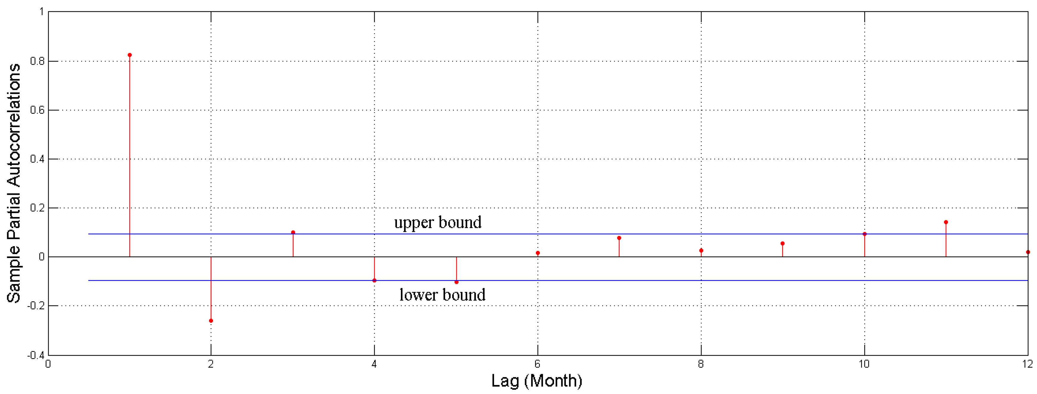
In this study, the prediction model has a “input-output” time-lag structure, where output is groudwater depth for t time step and inputs are goundwater depth in t-n previous months. Here, in order to determin the lag time n, a partial autocorrelation function (PACF) was carried out to test the correlation of the examined time series [37]. Figure 6 plots the PACF of groundwater process with 95% confidence bounds (blue solid line). The correlation pattern indicated that a strong correlation exists among groundwater depths in consecutive months, which proves the feasibility of forecasting groundwater depth using groundwater depth in previous months. Further, an autoregressive model with lag time 5 may be warranted for this time series, since there are notable partial autocorrelation for the lag 1 to 5.
3.3. ANN Training Model
ANN is a classic learning system inspired by biological neural networks. An ANN model has a multi-layer feedward structure connected by several nodes in each layer. Each node is a processer for “input-output” calculation. By parallel and massive iteration in the network, a convergent stable “input-output” structure may be achieved through a procedure known as model training. The goal of ANN is to find a function that fits given datasets best.
ANN is more effective in extracting and expressing hidden non-linear input-output relationships than traditional algorithms. Nevertheless, the flexibility of ANN structure also brings difficulties in model tuning. Improper settings of network structure or nodes may lead to deterioration in fitting performance, such as overfitting or underfitting. Evolutionary algorithms such as genetic algorithm (GA) particle swarm algorithm (PSO) and ant colony algorithm (ACA) have been emploryed in ANN model for parameter optimization and achieve improvement in model efficiency. As discussed above, the lag time of model structure is five, denoting the input variables (which is represented by input node in ANN) are previous five months data of each target output. Therefore, the input and output node numbers are 5 and 1 in ANN model structure. Node numbers of hidden layer is dependent on input and output node numbers as well as data feature. With the increase of node numbers, the model will be trained to fit more details but the generalization ability might decrease accordingly. Here the initial node number was set to be 25. Therefore, a (5:25:1) ANN model with 5 nodes of input layer, 25 nodes in hidden layer and 1 node of output layer was established as initial model structure. The node number of hidden layer is optimized by numeration from 25 to 5 with decremental step of 1. A genetic algorithm was combined in the node weight values of hidden layer in model calibration.
The data used to construct or discover a predictive model is called a training set, while data used to assess the model is called a test set. The quantity of training set and test set samples should be reasonably divided to assure the objectivity of both training and test procedures. Since we have 444 months of groundwater data sets, we defined a 3:1 ratio for training and test set samples. Specifically, groundwater depth data from 1974 to 2001 is training set, while data from 2002 to 2010 is test set.
3.4. SVM Training Model
3.4.1. SVM Algorithm
SVM is a machine learning theory based algorithm. SVM does not have a pre-determined structure, while the training samples are judged by their contributions. Only selected samples are contributed to the final model, which are the socalled “support vectors”. The SVM objective function can be expressed as:
where denotes direction vector, C denotes adjustment factor, and are slack variables, represents mapping input vector to high dimensional hyperspace, is intercept of regression function and is non-sensitivity coefficient. The former part of objective function represents the model complexity, while the latter part represents fitting error. In SVM theory, the model reaches best performance when the sum is minimized. SVM models seek the simultaneous optimum of model generalization performance and fitting performance.
The SVM model is a high dimensional quadratic programming problem. To avoid “dimensional disaster”, a kernel function is introduced to convert high dimensional computing into low dimensional computing. Generic kernel functions include linear, radial basis function (RBF), Gaussian, polynomial, and other kernel functions. Among them, the RBF kernel is superior to the linear kernel when dealing with high dimensional complex samples; compared with Gaussian and polynomial kernel functions, the parameter of RBF kernel function is simple. Thus, the RBF kernel is often chosen to solve the SVM model, expressed as:
where parameter g is used to fit different samples distributions.
3.4.2. PSO Parameter Calibration Method
The effectiveness of SVM depends on the selection of objective function parameter C, kernel parameter and non-sensitivity coefficient . There is currently no widely accepted best way to optimize SVM parameters. Grid search (GS) with exponentially growing sequences of combination {C, g} is often applied [38]. Grid search is easy to implement but has low computing efficiency. Moreover, optimal result of grid search can only generate from existing grid combinations, while unknown possible better parameters can not be explored and discovered.
In this study, a PSO based parameter optimization method is adopted to search for best parameter combination. The performance of SVM is more sensitive to the value C and g than , for the range of is quite small that generally within interval [10−4, 10−1].
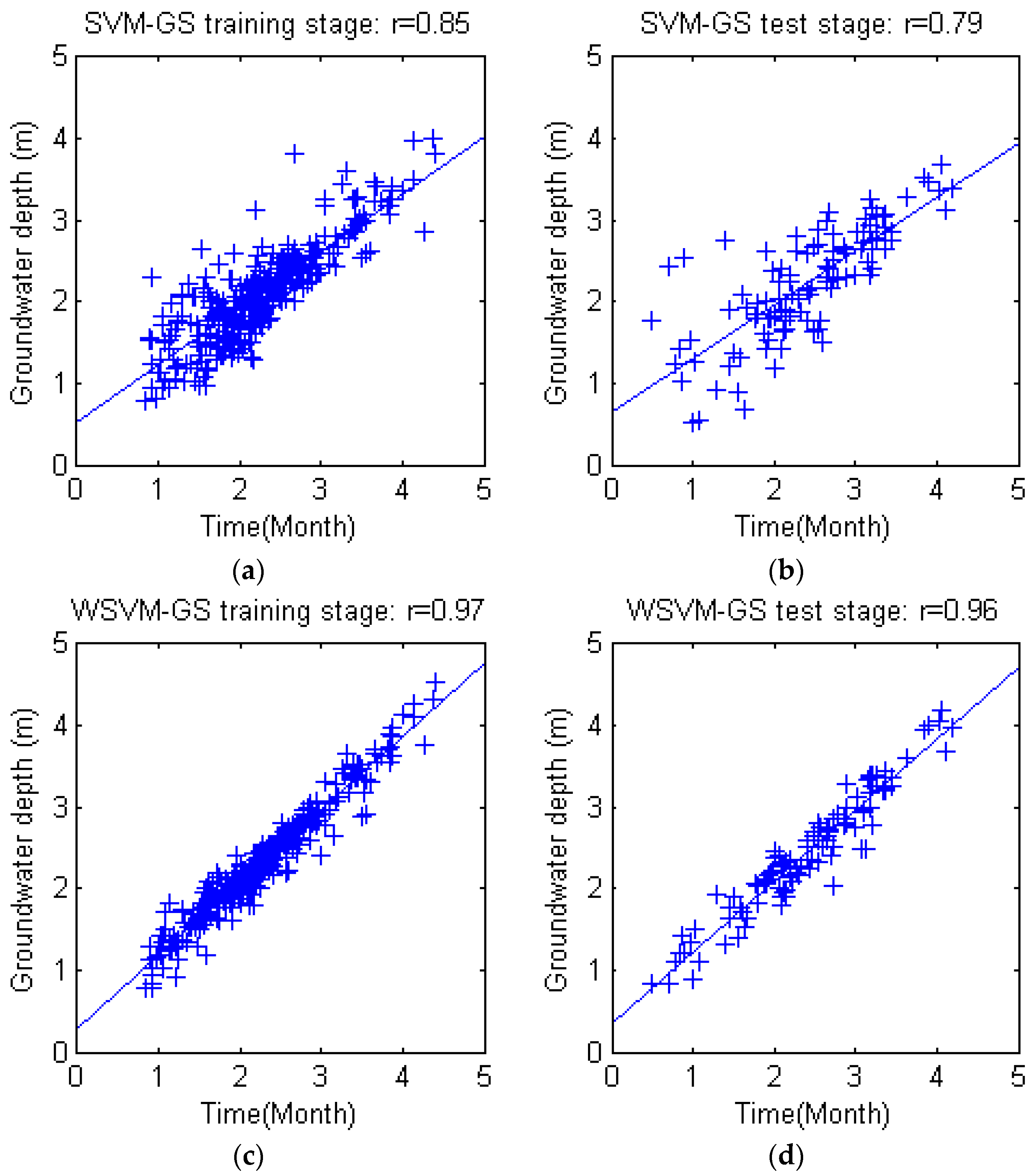
The PSO algorithm is derived from the migration mechanism of birds during foraging, which has advantages of fast convergence, efficient parallel computing and strong universality which is able to efficiently avoid local optimum [23,24]. Moreover, the iteration velocity of particle is influenced by the sum of current velocity, historical particle value, current global optimal value and random interferences, which avoids local optima to a large extent and improves search coverage and effectiveness. In this study, grid search also has been tried for comparison in this study—the PSO method is shown to be much more efficient. Parameter C was enumerated within set {2−5, 2−4, 2−3,… 25} and g in set {2−7, 2−6, 2−5,… 2}. Each combination was enumerated to determine the best parameter set. The training and test results of grid search based SVM and WSVM are shown in Figure 7. It is obvious that the PSO based SVM/WSVM simulation accuracy (shown in Section 4.1) bested the grid search based SVM/WSVM model.
3.4.3. Cross Validation
In machine learning algorithms, the basic purpose is fitting the model to training data, with the ultimate goal of making reliable prediction on unknown test data. However, favorable training performance does not always lead to reliable test performance. Overfitting is an example of this case. An overfitted model usually has minor training error but large test error, as the model learned too much unnecessary details from training data but fails to fit unknown test data. Overfitting may occur due to improper training mechanisms and internal parameters, which would lead to the more complicated and sensitive model. Although the proposed SVM model takes generalization performance and parameter calibration into account, overfitting may still occur caused by data bias in training, especially when the training set is small.
K fold cross validation mechanism was adopted to further avoid overfitting. The original training set was partitioned into k equally sized subsets. From the k subsets, a single subset was retained as a validation set, and the remaining k − 1 subsets were used as training set. The cross-validation process was then repeated k times (the folds), with each of the k subsets used as the validation data, alternatively. The final performance of a k fold model training was the average of validation performances in k subsets. Usually the value of k is determined by samples availability, generally from 2 to 10. Considering the overall training sample size is moderate, k is set to be 4 in this study.
The advantage of k fold cross validation mechanism is that in each round, the training sets and validation set are independent. Therefore, the performance is objective, creating a solid foundation for model optimization. Besides, the implementation of cross validation can improve efficiency of data utilization. In model configuration, the overall data set should be commonly divided into three independent sets: model calibration set, validation set, and test set. Sample sizes in each set might be small and lack of representative. By involving cross validation, the calibration set and validation set are combined as a whole, so the overall data would be divided into two sets. By the k fold of randomly dynamic division of training samples, the model can be more stable and objective.
In this study, the ratio of training samples and test samples is 3:1, indicating 75% training samples and 25% test samples. Considering 4 fold cross validation is applied on training set to train and calibrate the model, the calibration samples account for 75% of the overall training samples, and the rest 25% are validation samples. In summary, the ratio of calibration samples, validation samples, and test samples are 56.25%, 18.75%, and 25%.
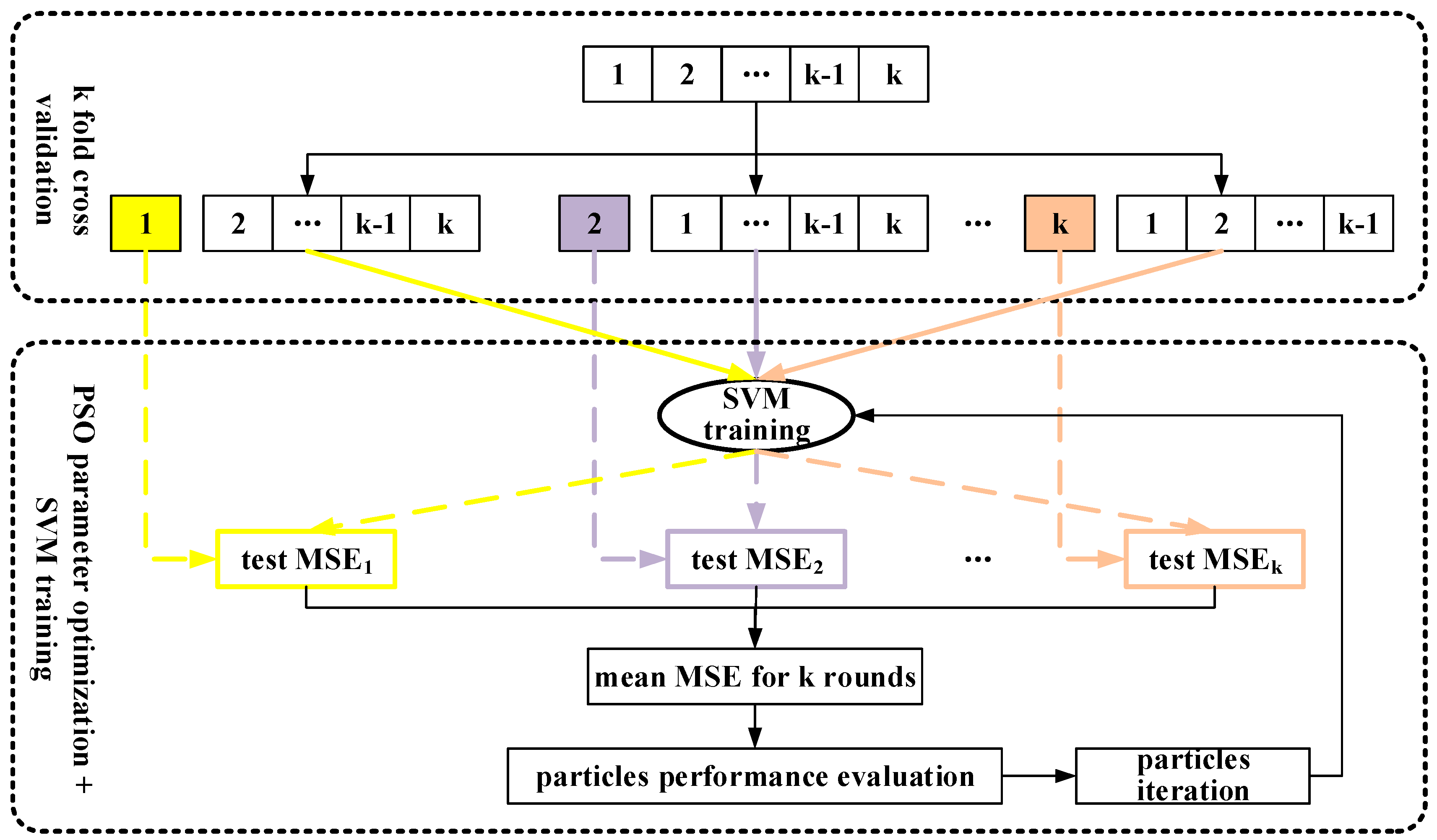
The final hybrid SVM model, which integrates SVM theory, PSO parameter optimization method and k fold cross validation was trained on the whole training set, as shown in Figure 8.
3.5. Wavelet Based Preprocess Analysis
Wavelet transform is used for de-noising, compression, and decomposition of data series. In wavelet transform analysis, a time series process is considered consisting of low frequency components and high frequency components. Low frequency component represents general and regulated features of time series, such as cyclical and seasonal trends, while the details and chaotic element is preserved in high frequency component. Similar with components seperation in time series analysis, the seperation of these features may be helpful to extract the inherent patterns of original time series.
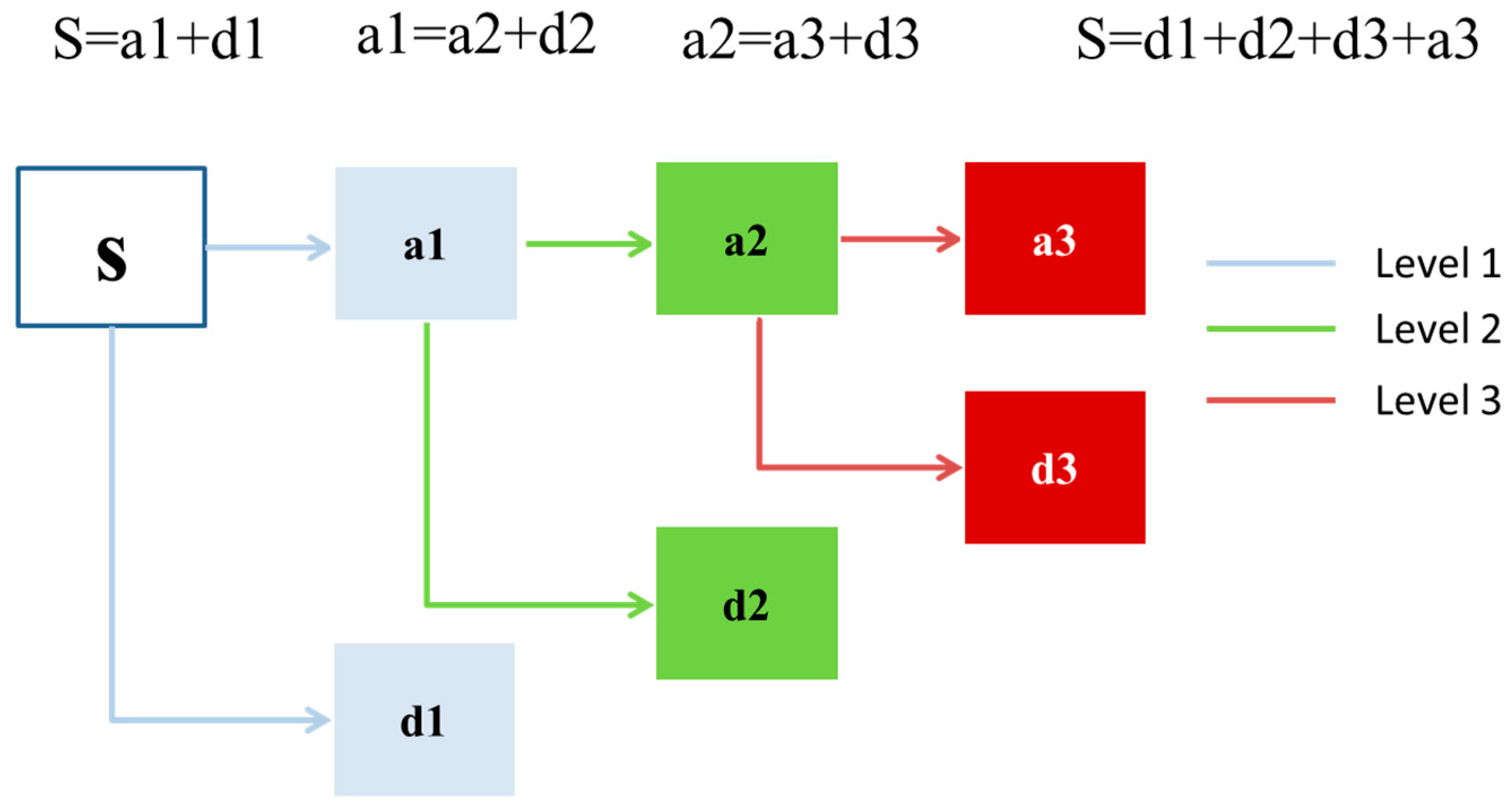
Discrete wavelet transform (DWT) is a method for seprating the low frequency and high frequency components into given layers. Mallat transform, proposed by Stephane Mallat in 1989 [39] has been the most practical and efficient method for DWT implementation. Figure 9 illustrated the framework of Mallat DWT theory. The original groundwater depth S passes through level one filter and emerges as two signals: low frequency component a1 and high frequency components d1, and this is called one level wavelet. Similarly, the decomposition process can be operated for n times, with low frequency components successively broken down into lower components, which is called n level DWT. Therefore, a DWT with n levels will generate n + 1 subseries, which consists of n high frequency and 1 low frequency subseries. The proper level n is determined by data series feature. If the data is chaotic which need intensive refining, the level is better to be larger. However, it is noted that increasing DWT level does not necessarily mean model performance improvement, for the error layers will also increase with level increase. In this study, several rounds of test were carried out that enumerating level from three to six, a three level DWT is shown to be best. Several types of wavelet functions can be used in DWT, including Meyer wavelet, Haar wavelet, Daubechies wavelet, ReverseBior wavelet, etc. In this paper, the Daubechies wavelet was chosen for its compact support and orthogonality, which has enormous potential in describing details of groundwater depth fluctuations accurately.
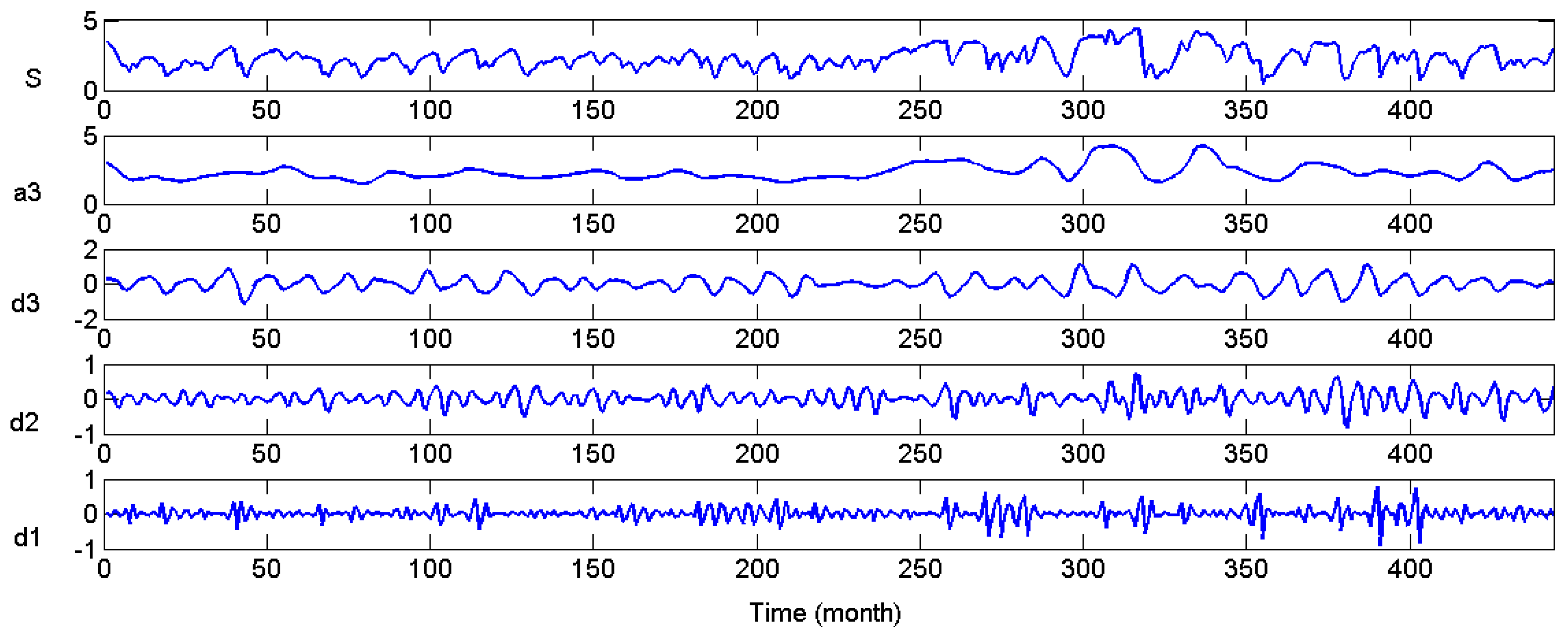
The three level DWT result is shown in Figure 10. The three level DWT decomposed groundwater depth (S) into low frequency subset (a3) and three high frequency subsets (d1), (d2) and (d3). Obviously, S = a3 + d1 + d2 + d3. The subseries show apparent differences from each other, but the feature of each subseries are much more orderly and consistent, which will facilitate the rules derivation for each subseries.
3.6. Model Verification
Relative absolute error (RAE), Pearson’s correlation coefficient (r), root mean square error (RMSE), and Nash-Sutcliffe efficiency (NSE) coefficient are employed as the performance evaluation criterion for comparison of ANN, SVM, WANN and WSVM models, as follows:
where and denote actual and estimated value of groundwater depth in time step i, respectively; and denote mean value of the actual and estimated value of groundwater depth in time step i, respectively; n is the number of samples.
RAE takes the total absolute error and normalizes it by dividing by the total absolute error of the predictor. RAE ranges from 0 to ∞. In a perfect prediction, RAE is equal to 0; the numerator value increases with the increase of model prediction error.
The coefficient r measures the linear relationship between observation and estimation values. The coefficient r ranges from −1 to 1. A value of 1 or −1 implies that a linear equation describes the relationship between and perfectly. A value of 0 implies that there is no linear correlation between and .
RMSE is frequently used in measuring standard deviation of differences between estimated values and observed values. The closer the RMSE is to 0, the less deviation there is between estimations and observations.
NSE is a coefficient particularly used to assess the predictive power of hydrologic models. NSE values ranges from −∞ to 1. An efficiency of 1 is a perfect match of model predictions to the observations. An efficiency of 0 indicates that model predictions are as accurate as the mean of the observed data, whereas efficiency less than 0 means the residual variance exceeds the data variance. Essentially, models with NSE in the (0, 1) range are feasible, otherwise the model is usually considered infeasible for application.
The criterion RAE and r can describe the aggregated fitting performance for all samples; while RMSE and NSE reflect the fluctuation of time series trend which focus more on the track of extreme values. By the criterions above, model performance can be characterized from different point view. However the premise of evaluation is that the training set and test set are assured to be representative [40,41]. In order to test the objectivity and stability of proposed model, more rounds of model procedures were carried out by exchanging and deleting the training and test samples. The stability test is applied on the best model, as discussed in Section 4.3.2.
4. Results and Discussion
4.1. Model Fitting and Test Results
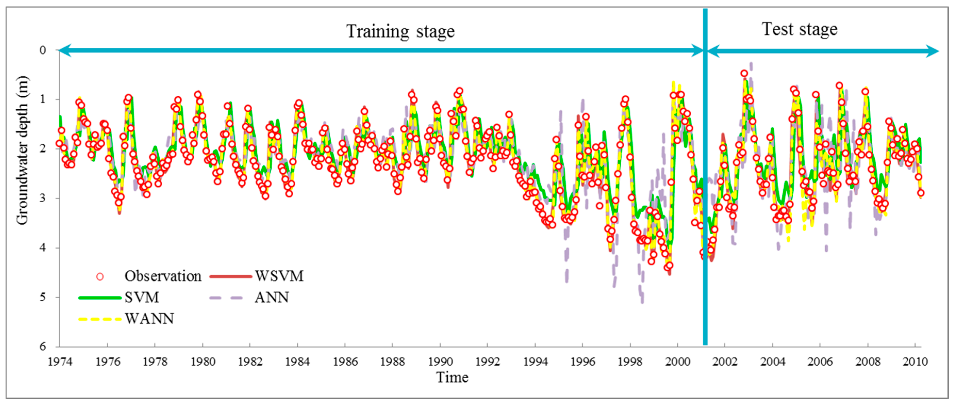
The fitting and test results of four models and actual groundwater depth series are shown in Figure 11. Scattered distribution of predicted values and observed values with linear regression trends are plotted in Figure 12. The figures show clearly that the overall performance of WANN and WSVM are superior to ANN and SVM models. The trends of WANN and WSVM have better agreement with observations than ANN and SVM models in Figure 11; scatter plots show that the estimation of WANN and WSVM are closely around 1:1 curve with few outliers in Figure 12. Moreover, Figure 11 indicates that ANN model performs less well than the SVM model, particularly in the sudden rises and declines during 1995 to 2008. Further indication is needed to distinguish differences between WANN and WSVM, for they have the same r coefficient in both training and test stages according to Figure 12e–h.
4.2. Comparative Discussion of Model Results
Table 2 gives the evaluation coefficients of each model in training and test stages. It can be inferred from the criterions in Table 2 that the WSVM model improves over the WANN model, for its RMSE is smaller and NSE is larger than WANN model. Therefore, model performance can be preliminarily ranked from high to low as: WSVM > WANN > SVM > ANN.
Moreover, we listed the gaps of each criterion between training stage and test stage to measure the generalization ability for each model. Model performance gap and generalization ability have an inverse relationship. Therefore, according to Table 2, the generalization ability of the four models is ranked as: WSVM > WANN > SVM > ANN, consistent with their prediction performance rank.
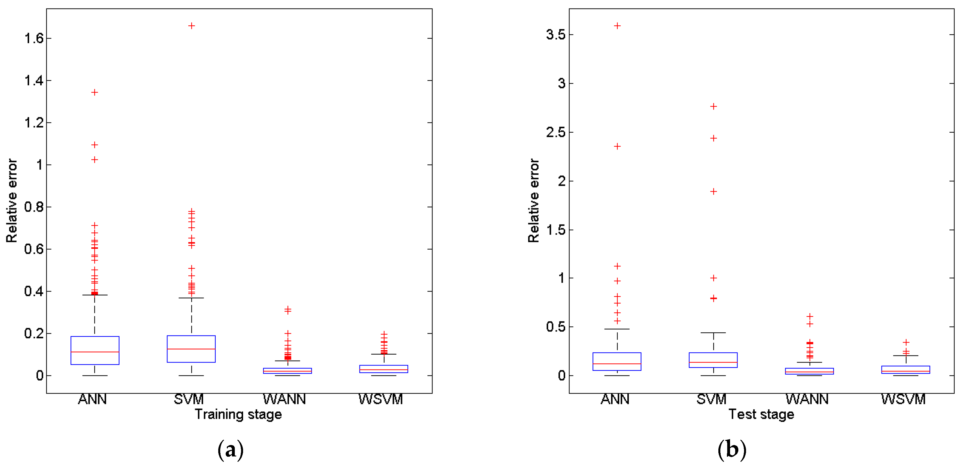
For prediction models, system stability is a crucial criterion. If prediction error fluctuates wildly when applied to different unknown scenarios, the model is usually considered impracticable even if the average error is quite low, because we cannot control the risk in real time operation. Here to avoid the limitation of single evaluation criterion, we further calculated relative error for each test data to examine the models stability using formula (7):
The relative errors of the four models are plotted in Figure 13. Upper bounds of relative error vary greatly among the four models. The relative error of WSVM is closely arranged with fewer outliers comparing with the other three models, which shows the WSVM model is more reliable in both precision and stability. The WSVM model has significant advantages over the other three models.
The comprehensive comparative analysis has two implications:
- From theoretical point of view, the SVM model has better performance than the ANN model in this case. Models with SVM theory, for both raw data and wavelet preprocessed data, have more accurate precision than that with ANN theory. The focus on generalization ability of SVM model, as explained in 3.5, is a critical issue for overcoming the ANN model. The PSO parameter calibration and cross validation mechanism further guaranteed its prediction performance.
- From model architecture point of view, the wavelet based preprocess profoundly improves model performance. The essential improvement of WANN and WSVM is attributed to the wavelet based preprocess of raw groundwater depth data. The wavelet based preprocess filters the original groundwater depth series into regulated subseries (Figure 10). The partition of raw data makes hybrid models (both WSVM and WANN) more capable of extracting those unknown patterns hidden in the groundwater fluctuations, which leads to more accurate prediction results. This is the reason for the substantial improvement of WANN and WSVM models. Although SVM theory is more efficient than ANN theory, the WANN model performs much better than SVM model. This illustrates that data preprocessing may be more important than the model itself in this case.
4.3. Discussion of WSVM Model
4.3.1. WSVM Model Performance
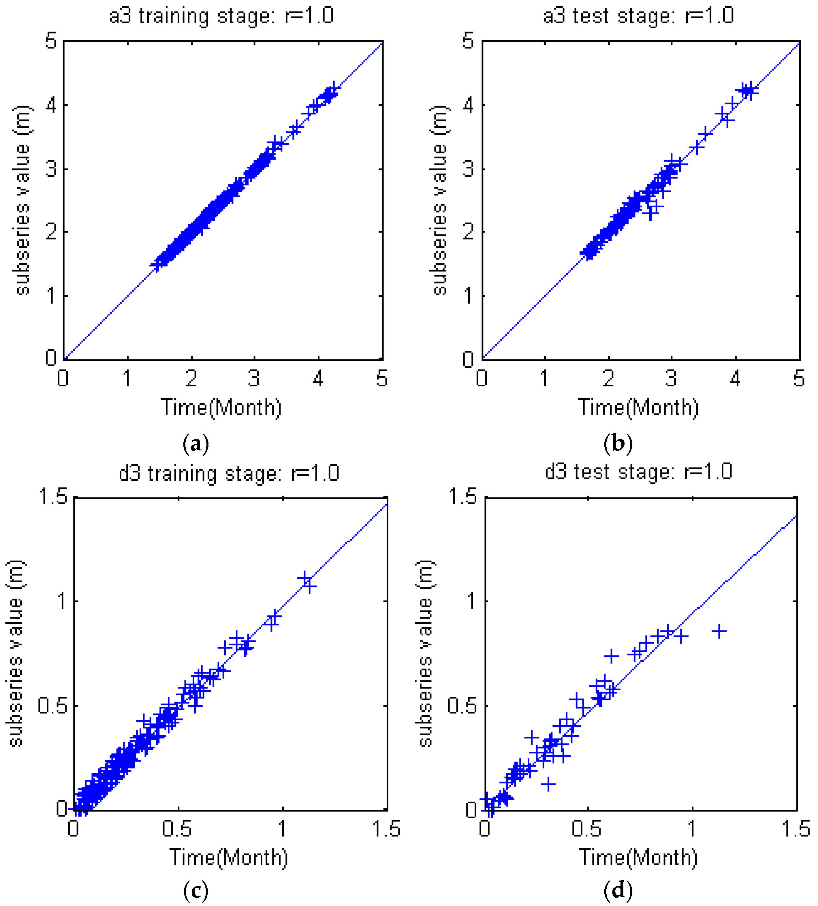
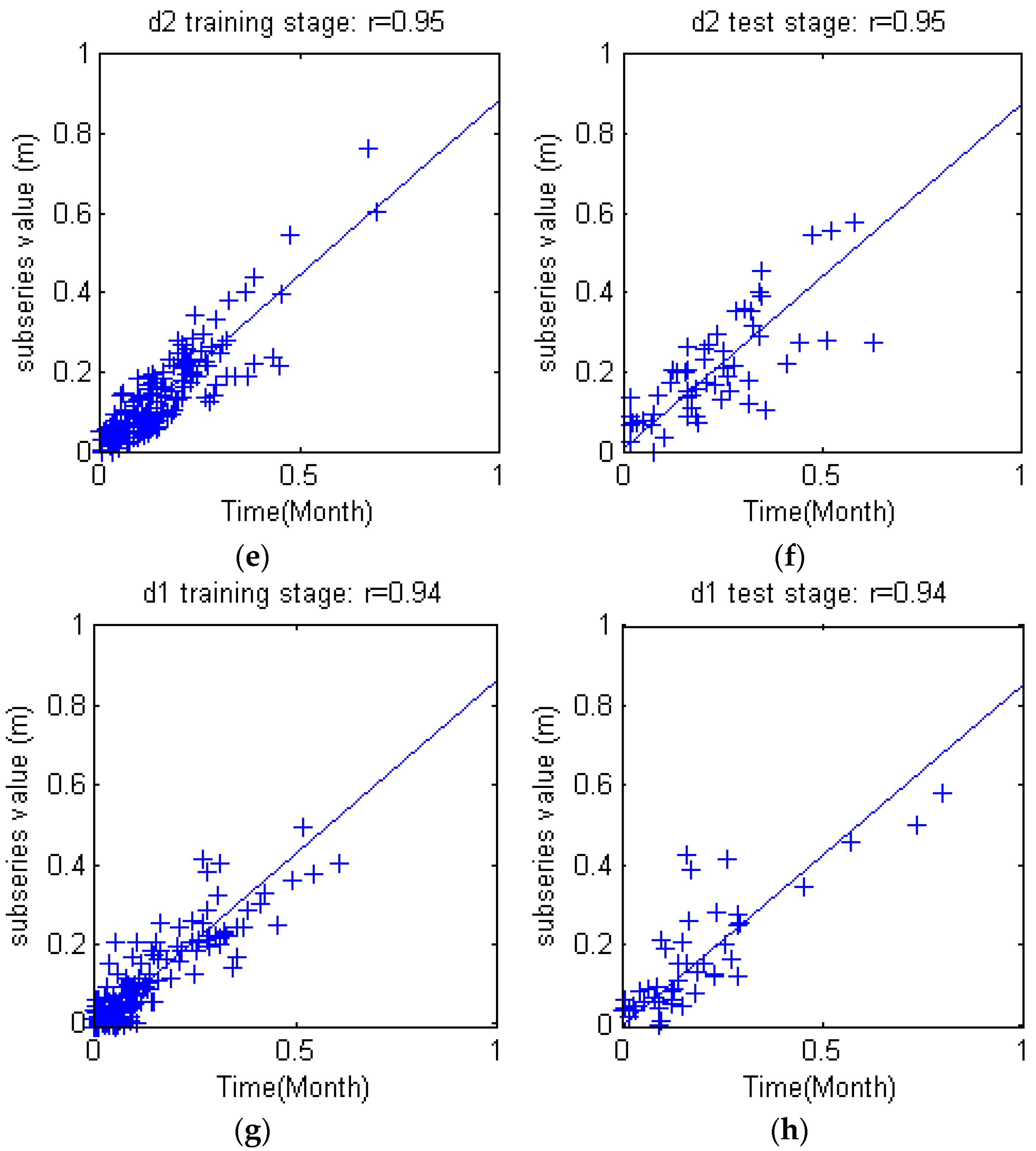
Since former analysis showed that WSVM is the best model among the four models compared, more detailed specifications WSVM are given and discussed. In WSVM, four subseries generated by the three level DWT are independently trained in SVM model. Table 3 gives the detailed model verification coefficients for each subseries. All subseries are quite consistent with original series, with r value and NSE value approaching 1 and RMSE value approaching 0. The gaps between training stage and test stage are close to 0 in each subseries, indicating little overfitting. Subseries performance is even better than the reconstructed result shown as WSVM in Table 2.
Figure 14 shows scattered plots for simulated data and original subseries data of each subseries. With the increase of subseries frequency, the fitting and test performances tend to decrease slightly. For low frequency subseries a3, simulated results fit raw subseries data precisely; when it comes to d2 and d3 subseries, the fitting curve gradually deviated from 1:1 line, and the samples are getting diverse. Subseries d4 indicates an increasing simulating error. The differences can be explained by the wavelet analysis theory: stable characteristics of original time series were preserved in low frequency subseries a3; high frequency subseries comprise complicate information and noises, which are therefore difficult for characteristics extraction. The importance of data preprocessing is also shown here: even for the carefully calibrated WSVM model, data “quality” still profoundly affects model performance.
4.3.2. Stability Test of WSVM Model
The stability test of WSVM model is carried out based on two schemes by samples processing:
Scheme 1: Change the samples order by reversing the two halves of original time series data, and then still use the 3:1 ratio to divide training and test samples. In this way, the training samples include groundwater depth from 1974 to 1983, and 1994 to 2010; test samples are groundwater depth from 1984 to 1993.
Scheme 2: delete the last 25% of original training samples (84 samples from 1995 to 2001) from training set, and take them as test samples. Therefore, the ratio between training set and test set is changed from 3:1 to approximately 1.29:1.
WSVM model is trained and tested independently on the two schemes. The fitting and test results of the two schemes are shown in Figure 15.
It is intuitively indicated that WSVM model performs still satisfying in the two schemes. The trend of WSVM prediction result is closely accordant with observed data in both schemes. To quantify the training and prediction performance, Table 4 is given with evaluation coefficients in training and test stages.
Comparison between values in Table 4 and Table 2 illustrates that both scheme 1 and scheme 2 achieved equally favorable performance as previous model. This experiment proves that the proposed WSVM model can maintain its high efficiency when substituting training samples, or decreasing training samples (to a moderate extent that would not affect the representative of training set). It is probably attributed to the solid mathematical processes in the hybrid model: data preprocess, parameter optimization, cross validation mechanism and SVM generalization. These elements provide strong guarantee for the flexibility and adaptability in capturing inherit features of non-stationary time series.
5. Conclusions
The potential of wavelet preprocessed Support Vector Machine (WSVM) model for monthly groundwater depth prediction during 1974 to 2010 in Mengcheng County were investigated in this study. The coupled WSVM model was developed by combining DWT and Support Vector Machine. The input variables lag times were derived from partial autocorrelation function of groundwater depth time series. A three level DWT is taken to preprocess and decompose the original groundwater level time series into four subseries with different frequencies. PSO based parameter calibration and 4 fold cross validation mechanisms were adopted into the hybrid WSVM model. The WSVM model was compared with ANN, SVM and WANN models using the same historic data. The WSVM model provided more accurate results. The RAE, r coefficient, RMSE and NSE were 0.10, 0.99, 0.095 and 0.98 in training stage and 0.20, 0.97, 0.18 and 0.94 in test stage, which largely bested the other models. WANN was close to WSVM models in some single coefficients but the relative error distribution demonstrated that the WSVM model has more stable performance. Through the use of three level DWT, the groundwater depth series was decomposed into four subseries with better stationary for model training. This facilitated the extraction of mainstream components thus significantly improved prediction performance.
By comprehensive comparisons of the four models and subseries of WSVM model, wavelet preprocessing helps provide quite good forecasts of monthly groundwater depth. The proposed hybrid model WSVM is a promising and practical method for monthly groundwater prediction. One possible future research from this study is developing multi lead time prediction models. Different from the one lead time prediction proposed in this study, the dilemma for multi lead time prediction might be how to deal with and avoid error accumulation of each time step. For rolling predictions, further lead time prediction is established on previous prediction; however, the previous prediction may probably have error which will mislead future prediction. Thus, the trade-off between information value and risk should be analyzed carefully.
Acknowledgments
This research was supported by National Science Fund of China (No. 51509001), Natural Science Fund of Anhui Province (No. 1608085QE112) and Talent Training Program for Universities of Anhui Province (No. gxyqZD2017019).
Author Contributions
Ting Zhou designed and implemented the model frameworks, and wrote the paper; Faxin Wang provided and analyzed the groundwater historic data and background of study area; Zhi Yang analyzed the data and revised the paper.
Conflicts of Interest
The authors declare no conflicts of interest.
References
- Ebrahimi, H.; Rajaee, T. Simulation of groundwater level variations using wavelet combined with neural network, linear regression and support vector machine. Glob. Planet. Chang. 2017, 148, 181–191. [Google Scholar] [CrossRef]
- Chitsazan, N.; Tsai, F.T.C. A Hierarchical Bayesian Model Averaging Framework for Groundwater Prediction under Uncertainty. Groundwater 2015, 53, 305–316. [Google Scholar] [CrossRef] [PubMed]
- Lo, M.-H.; Famiglietti, J.S.; Yeh, P.J.F.; Syed, T.H. Improving parameter estimation and water table depth simulation in a land surface model using GRACE water storage and estimated base flow data. Water Resour. Res. 2010, 46, 1–15. [Google Scholar] [CrossRef]
- Chang, F.J.; Chang, L.C.; Huang, C.W.; Kao, I.F. Prediction of monthly regional groundwater levels through hybrid soft-computing techniques. J. Hydrol. 2016, 541, 965–976. [Google Scholar] [CrossRef]
- Yan, Q.; Ma, C. Application of integrated ARIMA and RBF network for groundwater level forecasting. Environ. Earth Sci. 2016, 75, 1–13. [Google Scholar] [CrossRef]
- Adamowski, J.; Chan, H.F.; Prasher, S.O.; Ozga-Zielinski, B.; Sliusarieva, A. Comparison of multiple linear and nonlinear regression, autoregressive integrated moving average, artificial neural network, and wavelet artificial neural network methods for urban water demand forecasting in Montreal, Canada. Water Resour. Res. 2012, 48, 273–279. [Google Scholar] [CrossRef]
- Bourennane, H.; King, D.; Couturier, A. Comparison of kriging with external drift and simple linear regression for predicting soil horizon thickness with different sample densities. Geoderma 2000, 97, 255–271. [Google Scholar] [CrossRef]
- Sahoo, S.; Jha, M.K. Groundwater-level prediction using multiple linear regression and artificial neural network techniques, a comparative assessment. Hydrogeol. J. 2013, 21, 1865–1887. [Google Scholar] [CrossRef]
- Mirzavand, M.; Ghazavi, R. A Stochastic Modelling Technique for Groundwater Level Forecasting in an Arid Environment Using Time Series Methods. Water Resour. Manag. 2015, 29, 1315–1328. [Google Scholar] [CrossRef]
- Mogaji, K.A.; Lim, H.S.; Abdullah, K. Modeling of groundwater recharge using a multiple linear regression (MLR) recharge model developed from geophysical parameters, a case of groundwater resources management. Environ. Earth Sci. 2015, 73, 1217–1230. [Google Scholar] [CrossRef]
- Patle, G.T.; Singh, D.K.; Sarangi, A.; Rai, A.; Khanna, M.; Sahoo, R.N. Time series analysis of groundwater levels and projection of future trend. J. Geol. Soc. India 2015, 85, 232–242. [Google Scholar] [CrossRef]
- Kumar, A.R.S.; Sudheer, K.P.; Jain, S.K.; Agarwal, P.K. Rainfall-runoff modelling using artificial neural networks comparison of network types. Hydrol. Process. 2005, 19, 1277–1291. [Google Scholar] [CrossRef]
- Emamgholizadeh, S.; Moslemi, K.; Karami, G. Prediction the Groundwater Level of Bastam Plain (Iran) by Artificial Neural Network (ANN) and Adaptive Neuro-Fuzzy Inference System (ANFIS). Water Resour. Manag. 2014, 15, 5433–5446. [Google Scholar] [CrossRef]
- Dogan, A.; Demirpence, H.; Cobaner, M. Prediction of groundwater levels from lake levels and climate data using ANN approach. Water SA. 2008, 34, 199–208. [Google Scholar]
- Reuter, U.; Möller, B. Artificial Neural Networks for Forecasting of Fuzzy Time Series. Comput.-Aided Civ. Infrastruct. Eng. 2010, 25, 363–374. [Google Scholar] [CrossRef]
- Wood, D.; Dasgupta, B. An Innovative Tool for Financial Decision Making the Case of Artificial Neural Networks. Creat. Innov. Manag. 1995, 4, 172–183. [Google Scholar] [CrossRef]
- Krishna, B.; Rao, Y.R.S.; Vijaya, T. Modelling groundwater levels in an urban coastal aquifer using artificial neural networks. Hydrol. Process. 2008, 22, 1180–1188. [Google Scholar] [CrossRef]
- Katherasan, D.; Elias, J.V.; Sathiya, P.; Haq, A.N. Simulation and parameter optimization of flux cored arc welding using artificial neural network and particle swarm optimization algorithm. J. Intell. Manuf. 2014, 25, 67–76. [Google Scholar] [CrossRef]
- Mehdi, K.; Mehdi, B. A novel hybridization of artificial neural networks and ARIMA models for time series forecasting. Appl. Soft Comput. 2011, 11, 2664–2675. [Google Scholar]
- Sonmez, M.; Akgüngör, A.P.; Bektaş, S. Estimating transportation energy demand in Turkey using the artificial bee colony algorithm. Energy 2017, 122, 301–310. [Google Scholar] [CrossRef]
- Leung, F.; Lam, H.; Ling, S.; Tam, P.K.S. Tuning of the structure and parameters of a neural network using an improved genetic algorithm. IEEE Trans. Neural Netw. 2003, 14, 79–88. [Google Scholar] [CrossRef] [PubMed]
- Vapnik, V.N. Statistical Learning Theory; John Wiley & Sons: New York, NY, USA, 1998. [Google Scholar]
- Sudheer, C.; Maheswaran, R.; Panigrahi, B.K.; Mathur, S. A hybrid SVM-PSO model for forecasting monthly streamflow. Neural Comput. Appl. 2014, 24, 1381–1389. [Google Scholar] [CrossRef]
- Wang, W.C.; Xu, D.M.; Chau, K.W.; Chen, S. Improved annual rainfall-runoff forecasting using PSO–SVM model based on EEMD. J. Hydroinform. 2013, 15, 1377–1390. [Google Scholar] [CrossRef]
- Kisi, O.; Cimen, M. Precipitation forecasting by using wavelet-support vector machine conjunction model. Eng. Appl. Artif. Intell. 2012, 25, 783–792. [Google Scholar] [CrossRef]
- Hou, Y.K.; Chen, H.; Xu, C.Y.; Chen, J.; Guo, S.L. Coupling a Markov Chain and Support Vector Machine for at-site downscaling of daily precipitation. J. Hydrometeorol. 2017, 18, 2385–2406. [Google Scholar] [CrossRef]
- Misra, D.; Oommen, T.; Agarwal, A.; Mishra, S.K.; Thompson, A.M. Application and analysis of support vector machine based simulation for runoff and sediment yield. Biol. Syst. Eng. 2009, 103, 527–535. [Google Scholar] [CrossRef]
- Yoon, H.; Jun, S.-C.; Hyun, Y.; Bae, G.-O.; Lee, K.-K. A comparative study of artificial neural networks and support vector machines for predicting groundwater levels in a coastal aquifer. J. Hydrol. 2011, 396, 128–138. [Google Scholar] [CrossRef]
- Shiri, J.; Kisi, O.; Yoon, H.; Lee, K.-K.; Hossein Nazemi, A. Predicting groundwater level fluctuations with meteorological effect implications—A comparative study among soft computing techniques. Comput. Geosci. 2013, 56, 32–44. [Google Scholar] [CrossRef]
- Amid, S.; Gundoshmian, T.M. Prediction of output energies for broiler production using linear regression, ANN (MLP, RBF), and ANFIS models. Environ. Prog. Sustain. Energy 2017, 36, 577–585. [Google Scholar] [CrossRef]
- Asnaashari, M.; Farhoosh, R.; Farahmandfar, R. Prediction of oxidation parameters of purified Kilka fish oil including gallic acid and methyl gallate by adaptive neuro-fuzzy inference system (ANFIS) and artificial neural network. J. Sci. Food Agric. 2016, 96, 4594–4602. [Google Scholar] [CrossRef] [PubMed]
- Suryanarayana, C.; Sudheer, C.; Mahammood, V.; Panigrahi, B.K. An integrated wavelet-support vector machine for groundwater level prediction in Visakhapatnam, India. Neurocomputing 2014, 145, 324–335. [Google Scholar] [CrossRef]
- Rathinasamy, M.; Rakesh, K.; Jan, A.; Sudheer, C.; Partheepan, G.; Jatin, A.; Boini, N. Wavelet-based multiscale performance analysis: An approach to assess and improve hydrological models. Water Resour. Res. 2014, 50, 9721–9737. [Google Scholar] [CrossRef]
- Maheswaran, R.; Khosa, R. Wavelet-Volterra coupled model for monthly streamflow forecasting. J. Hydrol. 2012, 450–451, 320–335. [Google Scholar] [CrossRef]
- Moosavi, V.; Vafakhah, M.; Shirmohammadi, B.; Behnia, N. A Wavelet-ANFIS Hybrid Model for Groundwater Level Forecasting for Different Prediction Periods. Water Resour. Manag. 2013, 27, 1301–1321. [Google Scholar] [CrossRef]
- Nourani, V.; Hosseini Baghanam, A.; Adamowski, J.; Kisi, O. Applications of hybrid wavelet–Artificial Intelligence models in hydrology, A review. J. Hydrol. 2014, 514, 358–377. [Google Scholar] [CrossRef]
- Janacek, G. Time series analysis forecasting and control. J. Time Ser. Anal. 2010, 31, 303. [Google Scholar] [CrossRef]
- Yao, C.; Wu, F.; Chen, H.J.; Hao, X.L.; Shen, Y. Traffic sign recognition using HOG-SVM and grid search. In Proceedings of the 12th International Conference on Signal Processing (ICSP), Hangzhou, China, 19–23 October 2014; pp. 962–965. [Google Scholar]
- Mallat, S. A theory for multiresolution signal decomposition: The Wavelet representation. IEEE Trans. Pattern Anal. Mach. Intell. 1989, 11, 674–693. [Google Scholar] [CrossRef]
- Panagoulia, D.; Tsekouras, G.J.; Kousiouris, G. A multi-stage methodology for selecting input variables in ANN forecasting of river flows. Glob. NEST J. 2017, 19, 49–57. [Google Scholar]
- Panagoulia, D. Artificial neural networks and high and low flows in various climate regimes. Hydrol. Sci. J. 2006, 4, 563–587. [Google Scholar] [CrossRef]
Figure 1.
Location of the study site and groundwater monitoring wells.

Figure 2.
Groundwater depth flucutuation in Mengcheng County, 1974–2010.

Figure 3.
Monthly precipitation and groundwater depth.

Figure 4.
Annual average groundwater depth.

Figure 5.
Flowchart of the modelling process for groundwater depth prediction.

Figure 6.
PACF of groundwater series with 95% confidence bounds.

Figure 7.
Scatter plot of simulated data and observed data for each model (a) SVM-GS training stage; (b) SVM-GS test stage; (c) WSVM-GS training stage; (d) WSVM-GS test stage.
Figure 7.
Scatter plot of simulated data and observed data for each model (a) SVM-GS training stage; (b) SVM-GS test stage; (c) WSVM-GS training stage; (d) WSVM-GS test stage.

Figure 8.
SVM training principle combined with PSO parameter optimization and k-fold cross validation.
Figure 8.
SVM training principle combined with PSO parameter optimization and k-fold cross validation.

Figure 9.
Architecture of three level discrete wavelet transform.

Figure 10.
Three level DWT of groundwater depth series of Mengcheng County.

Figure 11.
Prediction results for groundwater depth using four models.

Figure 12.
Scatter plot of simulated data and observed data for each model (a) ANN training stage; (b) ANN test stage; (c) SVM training stage; (d) SVM test stage; (e) WANN training stage; (f) WANN test stage; (g) WSVM training stage; (h) WSVM test stage.
Figure 12.
Scatter plot of simulated data and observed data for each model (a) ANN training stage; (b) ANN test stage; (c) SVM training stage; (d) SVM test stage; (e) WANN training stage; (f) WANN test stage; (g) WSVM training stage; (h) WSVM test stage.


Figure 13.
Relative error box plot of four models (a) training stage (b) test stage.

Figure 14.
Scatter plot of simulated data and observed data for each subseries in WSVM model (a) low frequency subseries a3 training stage; (b) low frequency subseries a3 test stage; (c) high frequency subseries d3 training stage; (d) high frequency subseries d3 test stage; (e) high frequency subseries d2 training stage; (f) high frequency subseries d2 test stage; (g) high frequency subseries d1 training stage; (h) high frequency subseries d1 test stage.


Figure 15.
Prediction results for groundwater depth (a) scheme 1 result; (b) scheme 2 result.


Table 1.
Specifications of observation wells.
| No. | Name | East Longitude | North Latitude | Start Time | End Time | Maximum Depth (m) | Minimum Depth (m) | Mean Depth (m) | Standard Deviation |
|---|---|---|---|---|---|---|---|---|---|
| 1 | Banqiaoji | 116.6944444 | 33.3272222 | 1974/8 | 2010/12 | 4.99 | 0.27 | 2.56 | 0.97 |
| 2 | Mengcheng south | 116.5736111 | 33.2469444 | 1974/8 | 2010/12 | 10.29 | 0.37 | 2.68 | 1.92 |
| 3 | Guoji | 116.4722222 | 33.0430556 | 1974/8 | 2010/12 | 5.64 | 0.06 | 2.14 | 0.90 |
| 4 | Lvwangji | 116.4850000 | 33.1658333 | 1974/8 | 2010/12 | 4.12 | 0.43 | 2.68 | 0.79 |
| 5 | Shunheji | 116.6433333 | 33.0191667 | 1974/1 | 2010/12 | 7.15 | 0.06 | 2.13 | 0.77 |
| 6 | Maji | 116.3252778 | 33.3269444 | 1979/3 | 2010/12 | 4.53 | 0.37 | 2.09 | 0.78 |
| 7 | Sanyiji | 116.4855556 | 33.0958333 | 1974/8 | 2010/12 | 5.64 | 0.06 | 2.14 | 0.90 |
| 8 | Tancheng | 116.5600000 | 33.4444444 | 1974/1 | 2010/12 | 5.27 | 0.38 | 2.30 | 1.10 |
| 9 | Wangji | 116.7266667 | 33.2477778 | 1974/1 | 2010/12 | 6.16 | 0.24 | 2.23 | 0.70 |
| 10 | Yuefang | 116.4177778 | 33.3477778 | 1979/3 | 2010/12 | 3.88 | 0.61 | 1.96 | 0.61 |
Table 2.
Evaluation coefficients for ANN, SVM, WANN and WSVM models.
| Model | Training Stage | Test Stage | Gap | |||||||||
|---|---|---|---|---|---|---|---|---|---|---|---|---|
| RAE | r | RMSE | NSE | RAE | r | RMSE | NSE | RAE | r | RMSE | NSE | |
| ANN | 0.55 | 0.82 | 0.43 | 0.64 | 0.64 | 0.72 | 0.60 | 0.44 | 0.09 | 0.10 | 0.17 | 0.20 |
| SVM | 0.58 | 0.85 | 0.41 | 0.68 | 0.64 | 0.78 | 0.53 | 0.56 | 0.06 | 0.07 | 0.12 | 0.12 |
| WANN | 0.13 | 0.99 | 0.080 | 0.99 | 0.21 | 0.97 | 0.20 | 0.93 | 0.09 | 0.02 | 0.12 | 0.06 |
| WSVM | 0.10 | 0.99 | 0.095 | 0.98 | 0.20 | 0.97 | 0.18 | 0.94 | 0.10 | 0.02 | 0.085 | 0.04 |
Table 3.
Evaluation coefficients for four subseries of WSVM model.
| Subseries | Training Stage | Test Stage | Gap | |||||||||
|---|---|---|---|---|---|---|---|---|---|---|---|---|
| RAE | r | RMSE | NSE | RAE | r | RMSE | NSE | RAE | r | RMSE | NSE | |
| a3 | 0.04 | 1.00 | 0.021 | 0.99 | 0.11 | 1.00 | 0.078 | 0.99 | 0.07 | 0.00 | 0.057 | 0.00 |
| d3 | 0.14 | 1.00 | 0.037 | 0.99 | 0.24 | 1.00 | 0.081 | 0.98 | 0.10 | 0.00 | 0.044 | 0.01 |
| d2 | 0.02 | 0.95 | 0.060 | 0.99 | 0.03 | 0.95 | 0.099 | 0.98 | 0.01 | 0.00 | 0.039 | 0.01 |
| d1 | 0.02 | 0.94 | 0.059 | 0.99 | 0.03 | 0.94 | 0.083 | 0.98 | 0.01 | 0.00 | 0.024 | 0.01 |
Table 4.
Evaluation coefficients for four subseries of WSVM model.
| Scheme | Training Stage | Test Stage | Gap | |||||||||
|---|---|---|---|---|---|---|---|---|---|---|---|---|
| RAE | r | RMSE | NSE | RAE | r | RMSE | NSE | RAE | r | RMSE | NSE | |
| 1 | 0.13 | 0.99 | 0.11 | 0.98 | 0.16 | 0.99 | 0.10 | 0.95 | 0.03 | 0.00 | 0.01 | 0.03 |
| 2 | 0.13 | 0.98 | 0.07 | 0.98 | 0.16 | 0.98 | 0.16 | 0.96 | 0.03 | 0.00 | 0.09 | 0.02 |
© 2017 by the authors. Licensee MDPI, Basel, Switzerland. This article is an open access article distributed under the terms and conditions of the Creative Commons Attribution (CC BY) license (http://creativecommons.org/licenses/by/4.0/).
Share and Cite
MDPI and ACS Style
Zhou, T.; Wang, F.; Yang, Z. Comparative Analysis of ANN and SVM Models Combined with Wavelet Preprocess for Groundwater Depth Prediction. Water 2017, 9, 781. https://doi.org/10.3390/w9100781
AMA Style
Zhou T, Wang F, Yang Z. Comparative Analysis of ANN and SVM Models Combined with Wavelet Preprocess for Groundwater Depth Prediction. Water. 2017; 9(10):781. https://doi.org/10.3390/w9100781
Chicago/Turabian StyleZhou, Ting, Faxin Wang, and Zhi Yang. 2017. "Comparative Analysis of ANN and SVM Models Combined with Wavelet Preprocess for Groundwater Depth Prediction" Water 9, no. 10: 781. https://doi.org/10.3390/w9100781
Note that from the first issue of 2016, this journal uses article numbers instead of page numbers. See further details here.