Parametric Modelling of Potential Evapotranspiration: A Global Survey

Abstract

We present and validate a global parametric model of potential evapotranspiration (PET) with two parameters that are estimated through calibration, using as explanatory variables temperature and extraterrestrial radiation. The model is tested over the globe, taking advantage of the Food and Agriculture Organization (FAO CLIMWAT) database that provides monthly averaged values of meteorological inputs at 4300 locations worldwide. A preliminary analysis of these data allows for explaining the major drivers of PET over the globe and across seasons. The model calibration against the given Penman-Monteith values was carried out through an automatic optimization procedure. For the evaluation of the model, we present global maps of optimized model parameters and associated performance metrics, and also contrast its performance against the well-known Hargreaves-Samani method. Also, we use interpolated values of the optimized parameters to validate the predictive capacity of our model against monthly meteorological time series, at several stations worldwide. The results are very encouraging, since even with the use of abstract climatic information for model calibration and the use of interpolated parameters as local predictors, the model generally ensures reliable PET estimations. Exceptions are mainly attributed to irregular interactions between temperature and extraterrestrial radiation, as well as because the associated processes are influenced by additional drivers, e.g., relative humidity and wind speed. However, the analysis of the residuals shows that the model is consistent in terms of parameters estimation and model validation. The parameter maps allow for the direct use of the model wherever in the world, providing PET estimates in case of missing data, that can be further improved even with a short term acquisition of meteorological data.

1. Introduction

Evaporation, which is an overall term covering all processes in which liquid water is transferred as water vapour to the atmosphere—definition already provided by ancient Greek philosophers [1]—is crucial element of multiple disciplines and an essential input of hydrological modelling, water resources management, irrigation planning, and climatological studies. Numerous efforts are reported in the literature, presenting different expressions of evaporation (including actual, potential, reference crop, and pan evaporation), based on different types of data. McMahon et al. [2,3] provide a major discussion of the background theory and definitions, as well as a critical assessment of the models developed so far.

Here, we emphasize the concept of potential evapotranspiration, PET, which is a theoretical quantity considered as “the rate at which evapotranspiration would occur from a large area completely and uniformly covered with growing vegetation, which has access to an unlimited supply of soil water, and without advection or heating effects” [4]. Since PET depends on soil properties, a better defined term is the so-called reference crop evapotranspiration, introduced by Doorenbos and Pruitt [5], and typically denoted as ET₀, which refers to the evapotranspiration from a standardized vegetated surface (i.e., actively growing and completely shading grass of 0.12 m height, surface resistance 70 s · m⁻¹, and albedo = 0.23). The globally accepted method for consistent estimation of PET is the Penman-Monteith (herein referred to as PM) equation, as formalized by the Food and Agriculture Organization (FAO), which is physically-based, and is therefore used as standard for comparisons with other, more simple approaches [6]. The major drawback for the generalized application of the PM method worldwide is the need of simultaneous measurements of four meteorological variables (air temperature, wind speed, relative humidity, and net radiation or, alternatively, sunshine duration), at the desirable spatial and temporal resolution.

To overcome the data requirements of the PM formula, a number of alternative approaches have been developed, which are typically classified into temperature-based and radiation-based; the former use only temperature observations, which are dense and easily accessible, while the latter also use values of extraterrestrial radiation (which is, in fact, periodic function of latitude and time). For many decades, such approaches have been widely applied for PET modelling worldwide using the standard “literature” values of the parameters involved in their governing equations. However, since these have been developed for specific studies, locations, and climatic conditions [7], their applicability outside of these distinct conditions usually result in unreliable predictions, introducing significant bias in PET estimations. For this reason, and particularly in the last years, significant attention is payed to local calibrations of empirical PET models, either by using direct PET observations at the field scale (e.g., lysimeter measurements) and/or against simulated PET data, provided by the PM formula. One of the first attempts is reported by Allen and Pruit [8], who calibrated and validated the Blaney-Criddle model against PM data, using local wind function and taking advantage of daily lysimeter measurements of alfalfa evapotranspiration. Similar calibration approaches were employed for all of the widespread PET formulas, such as the Thornthwaite, Blaney-Criddle and Priestley-Taylor (e.g., [9,10,11]), and other empirical expressions as well (e.g., [12]). Many recent publications also focus on the re-evaluation of the sole parameter of the Hargreaves equation against regional data, for a range of climatic regimes [13,14,15,16,17].

Although the spatial resolution and accuracy of meteorological data over the extended areas of the globe is not sufficient, current advances in remote sensing technologies allowed quite reliable estimations of PET by combining satellite and ground information [18]. Since gridded data of meteorological inputs and canopy characteristics is now easily accessible, several researchers employed PET estimations at large spatial scales, up to global [19,20,21,22], by employing scaling and interpolation techniques of varying physical complexity [23].

In two recent studies, Tegos et al. [24,25] calibrated a simplified radiation-based expression of the PM formula, using monthly meteorological data from a large number of stations over Greece and California, respectively. In both areas, the proposed formula, which contains either three or two free parameters, clearly outperformed other widely used methods, such as Hargreaves and Samani [26], Oudin et al. [12], and Jensen and Haise [27], as modified by McGuinness and Bordne [28]. Malamos et al. [29] also employed the parametric model at the daily scale, in the context of PET mapping over the irrigated plain of Arta, Western Greece.

In the present study, we employ the simplified (i.e., with two parameters) expression of the aforementioned model over the globe, by inferring its parameters through calibration against given Penman-Monteith values (next referred to as reference PET or ET₀). The meteorological inputs and ET₀ data are retrieved by the FAO CLIMWAT database that provides monthly climatic information at 4300 locations worldwide. A preliminary analysis of these data allowed explaining the major drivers of PET over the globe and across seasons. We perform extended analysis of the model inputs and outputs, including the production of global maps of optimized model parameters and associated performance metrics, as well as comparisons with a widely known formula by Hargreaves and Samani [26]. Finally, we use the interpolated values of the optimized parameter values to validate the predictive capacity of the model against detailed meteorological data, in terms of monthly time series, at several stations worldwide. The results are very encouraging, since even with the use of abstract climatic information for its calibration, the model generally ensures very reliable PET estimations. However, we have detected few cases where the model systematically fails to reproduce the reference PET, particularly across tropical areas. Except for these specific areas, the parameter estimations through the derived maps can be directly employed within the proposed formula, at both point and regional scales.

2. Theoretical Background

2.1. The Penman-Monteith Equation

The Penman-Monteith equation for estimating potential evapotranspiration from a vegetated surface, as formalized by Allen et al. [30], is:

$$\mathrm{PET}=\frac{1}{\lambda } \frac{\Delta \left(R_n-G\right)+{\rho }_{\alpha }{c}_{\alpha }\left(v_a^{*}-v_a\right)/r_a}{\Delta +\gamma \left(1+\raisebox{1ex}{$r_s$}\!\left/ \!\raisebox{-1ex}{$r_a$}\right.\right)}$$

(1)

where PET is the daily potential evapotranspiration (mm · d⁻¹); R_n is the net incoming daily radiation at the vegetated surface (MJ · m⁻² · d⁻¹); G is the soil heat flux (MJ · m⁻² · d⁻¹); ρ_a is the mean air density at constant pressure (kg · m⁻³); c_a is the specific heat of the air (MJ · kg⁻¹ · °C⁻¹); r_a is an aerodynamic or atmospheric resistance to water vapour transport for neutral conditions of stability (s · m⁻¹); r_s is a surface resistance term (s · m⁻¹); v_a* − v_a is the vapour pressure deficit of the air (kPa), defined as the difference between the saturation vapour pressure v_a* and the actual vapour pressure v_a; λ is the latent heat of vaporization (MJ · kg⁻¹); Δ is the slope of the saturation vapour pressure curve at specific air temperature (kPa · °C⁻¹); and, γ is the psychrometric constant (kPa · °C⁻¹). Given that the typical time scale of the PM equation is daily, all of the associated fluxes are expressed in daily or mean daily units.

We remark that the original Penman equation does not include the soil heat flux term, G, since Penman noted that, in his experiments, its impact in the energy balance was less than 2% [31]. Nevertheless, evaporation estimations are sensitive to G only when there is a large difference between successive daily temperatures [2]. In this respect, in most of practical applications this flux is not accounted for, thus leaving the net incoming daily radiation, R_n, as the sole energy term to be assessed; the latter is defined as the difference between incoming and outgoing radiation of short and long wavelengths.

Apart from the site location, expressed in terms of latitude, φ, the PM equation requires air temperature, relative humidity, solar radiation, and wind speed data for calculating the model’s variables. FAO provides detailed guidelines for the cases of proxy or missing meteorological information. A typical example is the determination of solar radiation from measured duration of sunshine or cloud cover. Moreover, FAO suggests using average daily maximum and minimum air temperatures, instead of mean daily temperature, to represent more accurately the non-linearity of the saturation vapour pressure—temperature relationship. If fact, the use of mean air temperature yields a lower saturation vapour pressure v_a*, and hence a lower vapour pressure difference v_a* – v_a, and lower reference evapotranspiration estimates [30].

2.2. The Parametric Formula

The parametric model, initially proposed by Koutsoyiannis and Xanthopoulos [32], and then formalized and implemented by Tegos et al. [24,25,33,34], provides PET estimates through calibration based on given (“reference”) PET data. The model performance was satisfying as the proposed framework provides consistent monthly PET estimates at point and especially at the regional scale. The most recent application was the daily and monthly implementation of the model for the PET mapping in an irrigated plain of Greece [29] and the investigation of trend analysis in Greece through the development of an R-script tool [35].

The mathematical expression of the parametric model, which is applicable to temporal scales from daily to monthly, is the following:

$$\mathrm{PET}=\frac{a{R}_a+ b}{1-cT}$$

(2)

where PET is the potential evapotranspiration in mm, R_a (kJ · m⁻²) is the extraterrestrial radiation, T (°C) is the mean air temperature, and a (kg · kJ⁻¹), b (kg · m⁻²), and c (°C⁻¹) are model parameters that should be inferred through calibration, against “reference” PET data, either modelled or measured. We remark that from a macroscopic point-of-view, the above parameterization has some physical correspondence to the PM equation, since the product a R_a represents the overall energy term (i.e., incoming minus outgoing solar radiation), parameter b represents the missing aerodynamic term, while quantity (1 − c T) is an approximation of the denominator term of the PM formula [24].

Equation (2) uses two explanatory variables, namely extraterrestrial radiation, R_a, and temperature, T, and thus it belongs to the so-called radiation-based approaches. The extraterrestrial radiation, defined as the solar radiation received at the top of the Earth’s atmosphere on a horizontal surface, is an astronomic variable, given by:

$$R_a=\frac{24\left(60\right)}{\mathsf{\pi }}{G}_{\mathrm{sc}}{d}_{\mathrm{r}}\left[{\omega }_{\mathrm{s}}\sin \left(\phi \right)\sin \left(\delta \right)+\cos \left(\phi \right)\cos \left(d\right)\sin \left({\omega }_s\right)\right]$$

(3)

where G_sc is the solar constant, with typical value 82 kJ · m⁻² · min⁻¹, d_r is the inverse relative distance of the Earth from the Sun, ω_s (rad) is the sunset hour angle, φ is the latitude (rad), and δ is the solar declination (rad). Variables d_r and δ are periodic functions of time, while ω_s is function of latitude and time. For details on computing the above astronomic variables, the reader may refer to the literature (e.g., [3]).

While for a given location the extraterrestrial radiation is a highly regular and fully predictable variable, thus only explaining the periodicity of PET, temperature exhibits quite irregular variability, thus explaining the fluctuations of PET, which is key component of the changing hydrological cycle, at all temporal scales, from daily to annual and even larger ones, i.e., overannual [36]. Following FAO recommendations, we can also take advantage from minimum and maximum daily temperature data, thus estimating the temperature term by the average:

$$T=\left(T_{\min }+T_{\max }\right)/2$$

(4)

This expression may be particularly useful in cases when records of mean daily temperature are missing, while average minimum (T_min) and maximum temperature (T_max) values are available.

2.3. Modified Parametric Model

It is well-known that the variability of daily and, even more, monthly PET is relatively small, if compared to other hydrometeorological variables, such as precipitation and runoff. For this reason, when attempting to estimate the model parameters a, b, and c through calibration, it is quite easy to achieve very high values of goodness-of-fitting criteria (e.g., efficiency), through combinations of parameter values that do not have physical sense. Additional uncertainty arises when the actual PET data is little informative to support the inference of the three parameters, e.g., due to limited length of associated meteorological data. In this respect, to avoid uncertainties due to “blind” calibration approaches or overfitting [37], we propose using the more parsimonious expression (also considering the minimum and maximum temperature, instead of the mean daily one):

$$\mathrm{PET}= \frac{a\prime R_a}{1- c\prime \left(T_{\min }+T_{\max }\right)/2}$$

(5)

which contains two instead of three parameters (parameter a′ in the numerator and parameter c′ in the denominator). Apparently, in the context of a calibration exercise using alternative expressions (2) and (5), the optimized values of c and c′ should be different.

The modified parameterization (Equation (5)) resembles the well-known approach by Priestley and Taylor [38], who developed a PET formula based on the original PM equation, but without the aerodynamic component; the latter was indirectly accounted by increasing the energy term by a factor of 1.26. For simplicity, this factor is generally considered as constant; however, several researchers have demonstrated that this exhibits quite significant seasonal and spatial variability (2).

3. The CLIMWAT Database: Preliminary Analysis

3.1. Database Overview

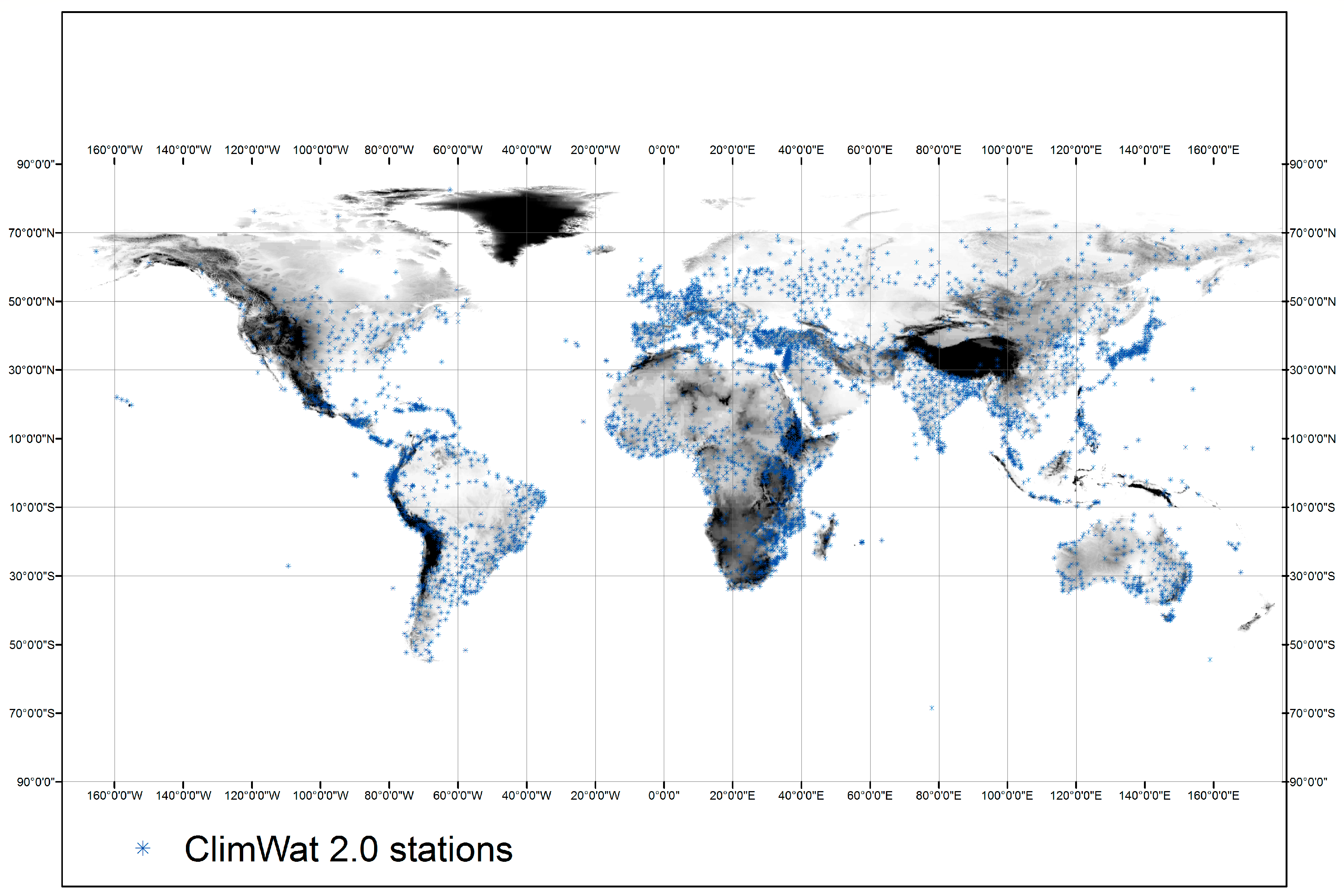
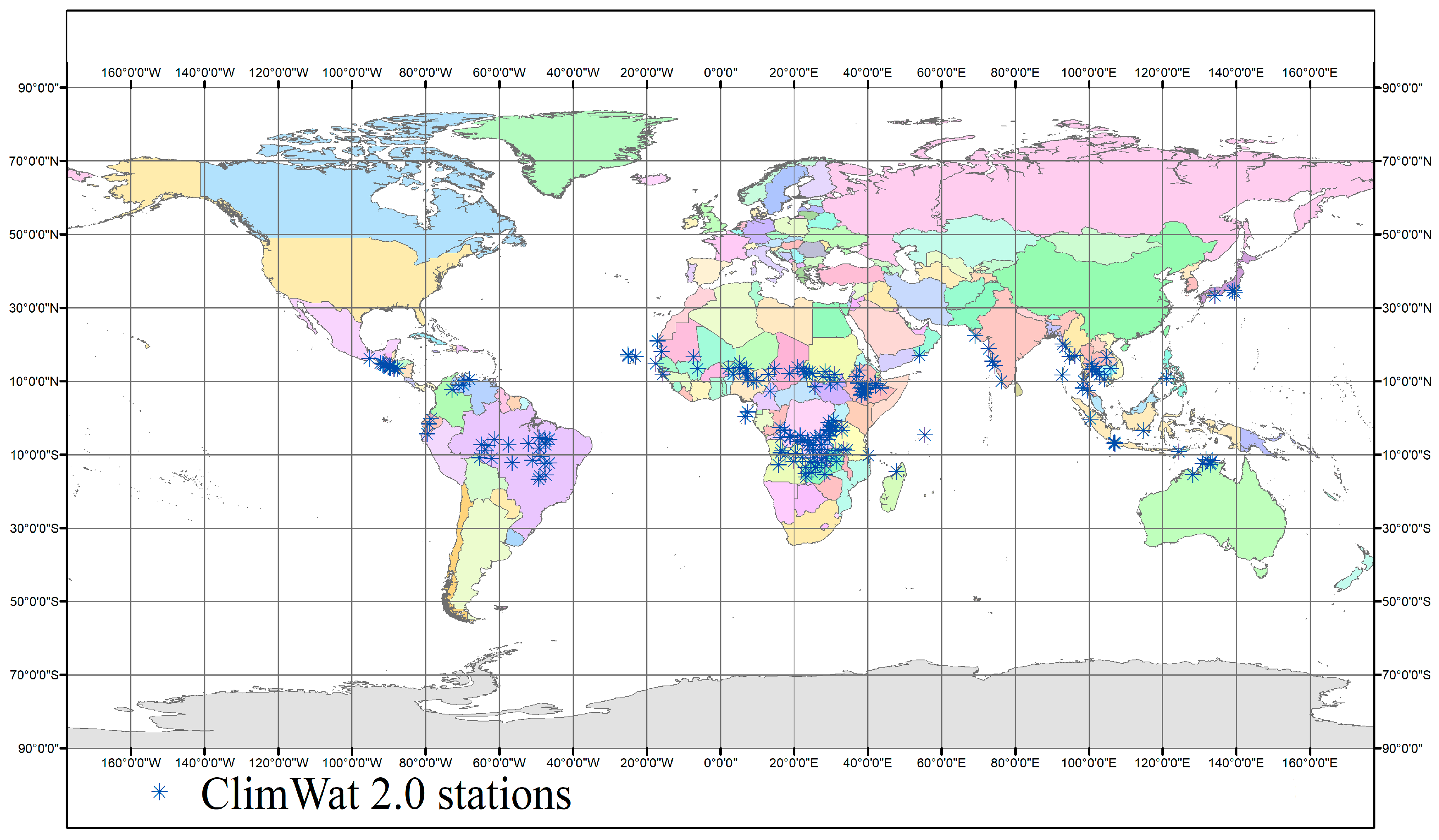
The CLIMWAT 2.0 database is a joint initiative by the Water Development and Management Unit and the Climate Change and Bioenergy Unit of FAO [39], which provides average monthly climatic data at 4300 stations (Figure 1, blue points), well-distributed worldwide. These data include monthly mean values of mean daily maximum and minimum temperature (°C), daily relative humidity (%), wind speed (km · day⁻¹), daily sunshine duration (h), daily solar radiation (MJ · m^-2), monthly rainfall, gross and effective (mm), as well as mean monthly ET₀ estimations through the Penman-Monteith formula.

The exceptionally large sample of climatic data allows for extracting useful conclusions about the major drivers of PET over the globe. In this context, we employed a comprehensive statistical analysis of reference PET data against the available meteorological variables, at both the annual and monthly scales. The outcomes of this analysis are summarized in Section 3.2 and Section 3.3, respectively.

3.2. Which Meteorological Drivers Explain Mean Annual PET over the Globe?

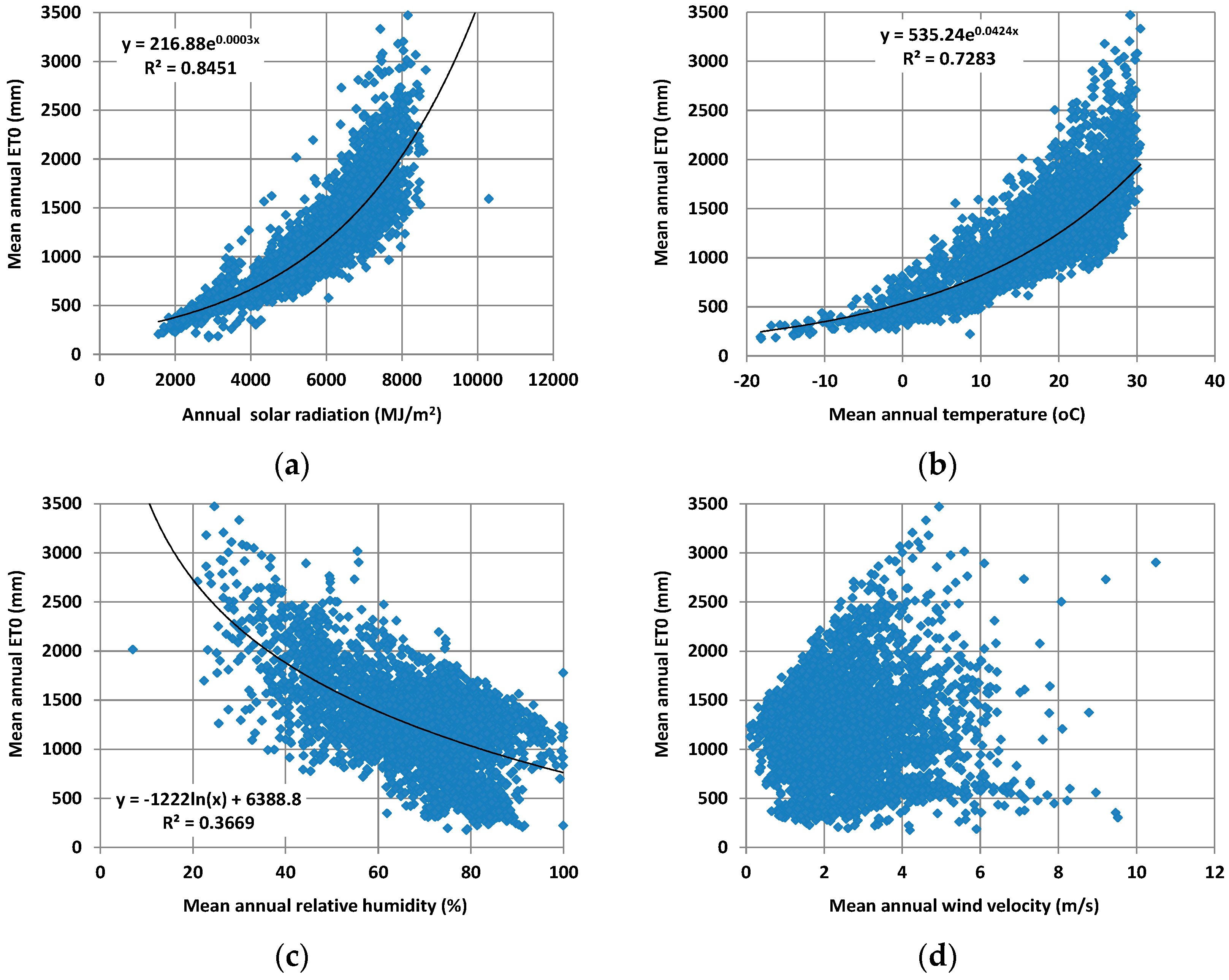
In order to answer this question, we plotted reference PET (i.e., ET₀) data against the four meteorological variables that are embedded in the Penman-Monteith equation, i.e., solar radiation, mean temperature estimated from Equation (4), relative humidity and wind speed, at the annual scale, and fitted the most suitable regression model.

Figure 2 illustrates that mean annual ET₀ over the globe is highly correlated with mean annual solar radiation and temperature, particularly when considering power-type or exponential regression functions. As expected, mean annual ET₀ is negatively correlated with mean relative humidity, while it seems uncorrelated to wind speed. It is worth mentioning that as the solar radiation and temperature increase, the variance of ET₀ increases significantly. Therefore, in order to reduce heteroscedasticity effects, it is essential considering at least two explanatory variables in the context of empirical PET modelling.

Figure 2 also demonstrates the variability of mean annual ET₀ against mean annual sunshine duration and annual extraterrestrial radiation, which are typically used instead of solar radiation, in PET estimations (given that solar radiation observations are generally sparse, due to the cost of associated equipment, i.e., pyranometers, radiometers or solarimeters). Surprisingly, the mean annual sunshine duration is slightly less correlated with mean annual ET₀ than extraterrestrial radiation, although the former is expected to be better estimator of the actual solar energy received in the Earth’s surface. This is a very important conclusion that confirms the suitability of radiation-based approaches, using both temperature and extraterrestrial radiation as explanatory variables of PET. However, it is essential remarking that the overall driver of PET and temperature as well is net solar radiation, which is a portion of the extraterrestrial one. Furthermore, the correlation between PET and temperature is so much significant only at coarse time scales, such as the annual one, while its correlation with the solar radiation remains significant, at all temporal scales [40].

3.3. How Well Do Extraterrestrial Radiation and Temperature Explain the Seasonal Patterns of PET?

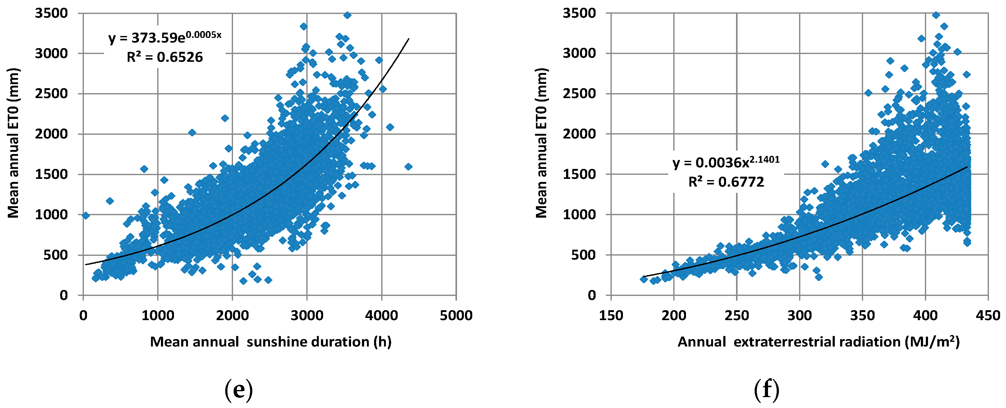
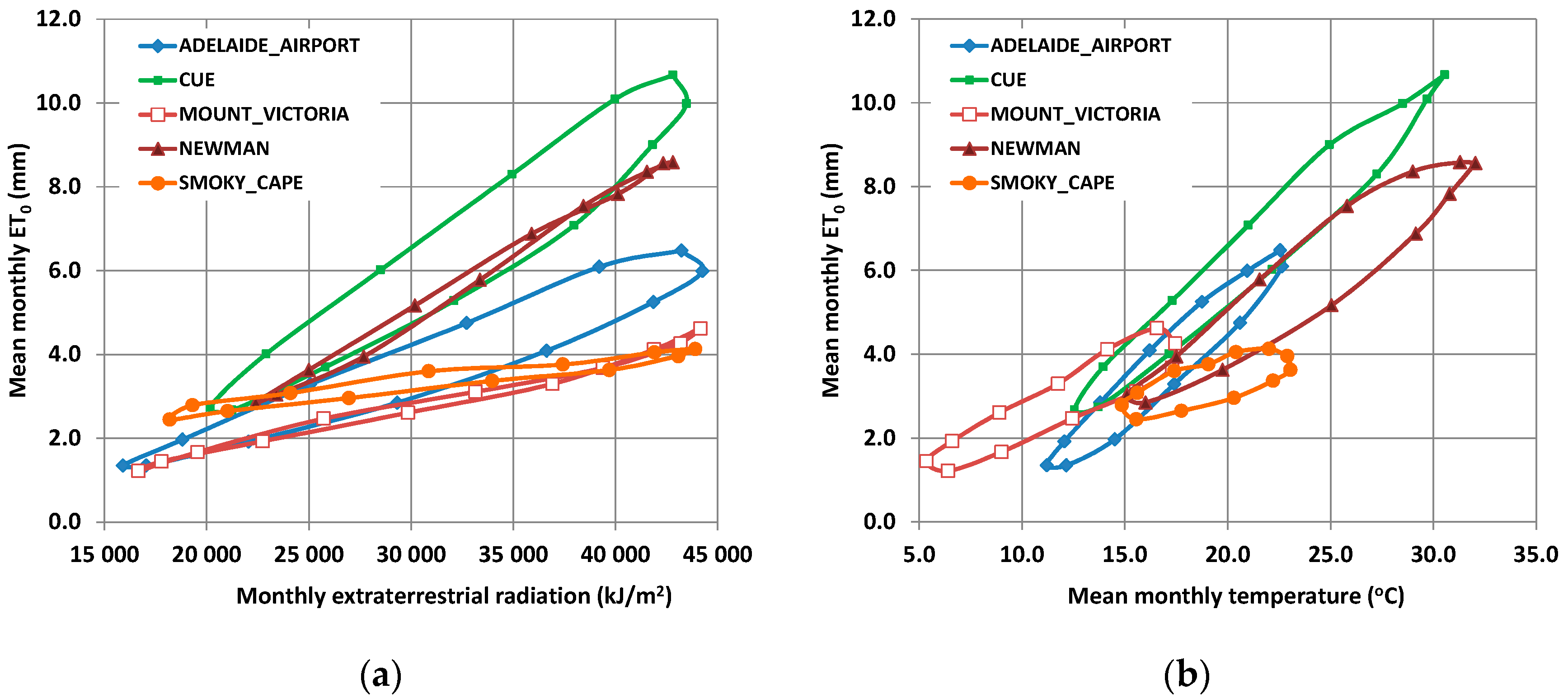
The key assumption of radiation-based models is that PET follows the seasonal patterns of extraterrestrial radiation, R_a, and temperature, T. In general, a loop-type shape exists between the mean monthly PET and the two aforementioned variables, due to the influence of thermal inertia, causing a delay in temperature changes against solar radiation changes across seasons. Apparently, due to the loop-shape relationship, the two pairs of variables are expected to be linearly correlated; actually, the more elongate the loop, the higher should be the correlation. In Figure 3, we plotted the relationships between monthly extraterrestrial radiation vs. mean monthly ET₀ and mean monthly temperature vs. ET₀, at five characteristic stations in Australia, exhibiting different hydroclimatic conditions, which confirm the above hypothesis. However, there are also cases where the shapes of T − ET₀ and R_a − ET₀ loops are irregular (nonconvex), thus resulting in very low, even negative, correlations. Such examples are shown in Figure 4, involving another set of stations in Australia.

In order to investigate whether extraterrestrial radiation and temperature actually explain the seasonal patterns of ET₀ over the globe, we formulated the linear regression models of mean monthly ET₀ against the two variables and calculated the coefficient of determination, r² (i.e., square of Pearson correlation coefficient), at the full sample of 4300 CLIMWAT stations.

Table 1. Ranges of coefficient of determination, r², between monthly ET₀ and the two explanatory variables, R_a and T, across the full sample of 4300 CLIMWAT stations.

T vs. ET0	Ra vs. ET0
	0–10%	10–20%	20–30%	30–40%	40–50%	50–60%	60–70%	70–80%	80–90%	90–100%	Total
0–10%	55	17	9	12	8	9	8	7	4	1	130
10–20%	38	11	7	4	11	8	3	3	5	3	93
20–30%	33	16	13	13	5	7	8	10	9	4	118
30–40%	36	14	24	10	7	5	12	12	8	15	143
40–50%	29	14	17	18	22	17	19	13	13	18	180
50–60%	34	10	17	16	17	28	26	21	26	31	226
60–70%	30	10	23	15	21	30	37	30	31	52	279
70–80%	45	11	15	19	28	20	44	48	77	135	442
80–90%	69	14	14	10	17	34	38	78	362	643	1279
90–100%	42	6	6	5	9	30	35	147	488	642	1410
Total	411	123	145	122	145	188	230	369	1023	1544	4300

summarizes the results, by means of number of stations corresponding to ranges of r², from 0–10% up to 90–100%. It is shown that ET₀ exhibits very high linear correlation, by means of r² values greater than 0.90 against both extraterrestrial radiation and temperature at only 642 out of 4300 stations (14.9%). This percentage rises up to 49.7% (2135 stations) is we consider a wider acceptable range for r², i.e., upper than 0.80.

On the other hand, at 443 stations over the globe (10.3%), the coefficient of determination is less than 0.50 against both explanatory variables. Apparently, the particular hydroclimatic regime at these areas does not allow representing PET through simplified radiation-based approaches, thus requiring either more complex parameterizations or additional variables to explain the seasonal patterns of PET due to energy or water limitations, i.e., relative humidity and/or wind speed [41,42]. PET has been proven sensitive to potential changes in climate in regions with a lower temperature, less solar radiation, and greater relative humidity, while the influence of the wind velocity and relative humidity in its estimation is supported by several studies [41,42,43,44,45,46,47].

An interesting remark is that in 42 stations (1% of the sample), a linear regression function of temperature against ET₀ ensures r² greater than 0.90, while at the same stations, the correlation between ET₀ and R_a is negligible (r² < 0.10). The opposite case, i.e., very high correlation of PET with R_a, while very low with T appears only once, thus it is statistically negligible. In this vein, we can consider a linear regression model between mean monthly T and ET₀ as benchmark to evaluate the performance of any other empirical model, which parameters are identified through calibration.

Nevertheless, although a number of studies present alternatives to the PM formula (e.g., [3,48]), based on the sensitivity of potential evapotranspiration to temperature and/or solar radiation, the major advantage of our approach is the ability of point calibration of the involved parameters [25].

4. Model Calibration

4.1. Evaluation Criteria

The large-scale PET information provided by FAO CLIMWAT database was used as reference data, for calibrating the parametric expression (Equation (5)), thus providing local estimations of parameters a′ and c′ at all station sites. For the evaluation of the model performance against reference PET (i.e., ET₀) we used the following statistical criteria:

• The coefficient of determination, most commonly referred to as efficiency or Nash-Sutcliffe efficiency:

  $$\mathrm{NSE}=1-\frac{{{\displaystyle \sum }}_{t=1}^T{\left({\mathrm{PET}}_{\mathrm{mod}}^t-{\mathrm{PET}}_{\mathrm{obs}}^t\right)}^2}{{{\displaystyle \sum }}_{t=1}^T{\left({\mathrm{PET}}_{\mathrm{obs}}^t-{\overline{\mathrm{PET}}}_{\mathrm{obs}}\right)}^2}$$

  (6)
• The mean absolute error:

  $$\mathrm{MAE}=\frac{{{\displaystyle \sum }}_{t=1}^T|{\mathrm{PET}}_{\mathrm{obs}}^t-{\mathrm{PET}}_{\mathrm{mod}}^t|}{T}$$

  (7)
• The relative bias:

  $$\mathrm{BIAS}=\frac{{{\displaystyle \sum }}_{t=1}^T({\mathrm{PET}}_{\mathrm{mod}}^t-{\mathrm{PET}}_{\mathrm{obs}}^t)}{{{\displaystyle \sum }}_{t=1}^T({\mathrm{PET}}_{\mathrm{obs}}^t)}$$

  (8)

where${\mathrm{PET}}_{\mathrm{obs}}^t$ is the ET₀ value, estimated by the PM formula at time step t, ${\mathrm{PET}}_{\mathrm{mod}}^t$ is the modeled value at time step t, ${\overline{\mathrm{PET}}}_{\mathrm{obs}}$ is the monthly average value of the reference PET, and T is total number of time steps (in the particular case, T equals the number of months, i.e., 12).

In calibrations, we used as performance measure the NSE, while the two other statistical metrics have been used for further evaluation. It is well-known that NSE ranges between −∞ and 1, with NSE = 1 indicating perfect fitting of the modelled against the given reference values. Due to the generally high linear correlations of R_a and T against ET₀, we only consider values greater than 0.70 as satisfying, whereas positive values less than 0.50 are only marginally accepted. On the other hand, negative NSE values are definitely unacceptable, since they indicate that the mean observed value is a better predictor than the simulated value. The mean absolute error and the bias are quite similar metrics, quantifying in absolute (i.e., mm/month) and relative (%) terms the deviation of the mean modelled ET₀ from the corresponding mean reference value, ${\overline{Q}}_{\mathrm{obs}}$.

4.2. Optimization Procedure

At each station, we formulated the associated global optimization problem, based on the given 12 monthly average values of ET₀, and using NSE as the objective function to maximize against parameters a′ and c′. Within calibration, we have considered a quite extended feasible space, by allowing a′ and c′ to vary within ranges [–0.02, 0.02] and [–5.0, 5.0], respectively. The global search was carried out with the evolutionary annealing-simplex algorithm, which is a heuristic technique that has been proved very effective on locating global optima in highly nonlinear spaces [49,50].

Due to the exceptionally large number of calibration problems to be solved at the full sample of 4300 stations, the computational procedure was automatized in a MATLAB environment.

4.3. Assessment against Linear Regression Estimations

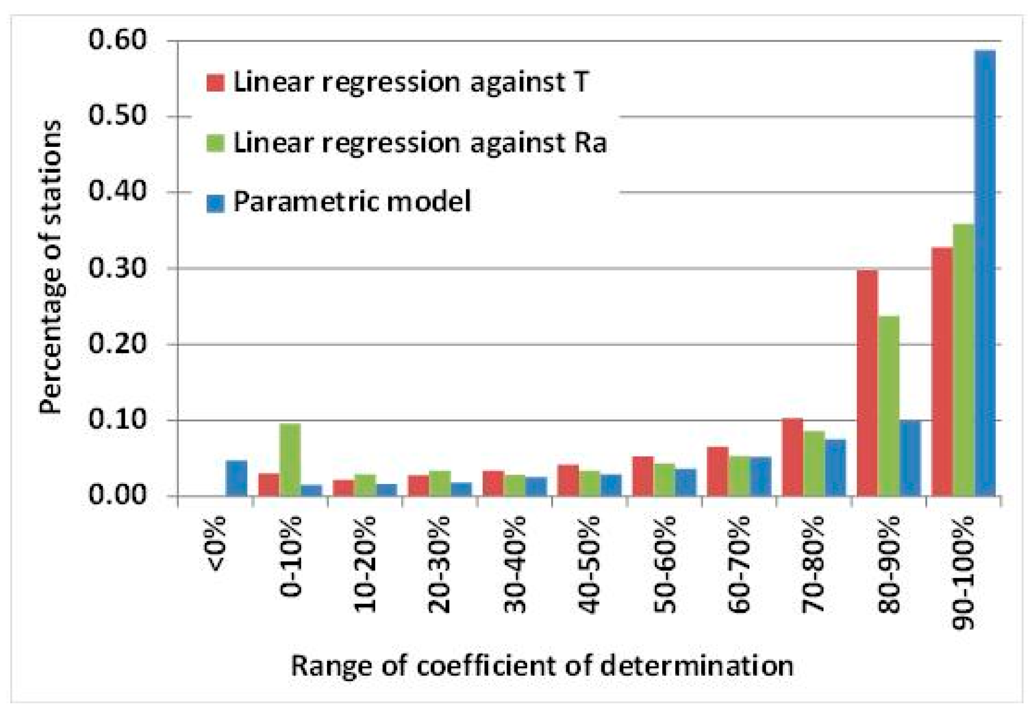
In order to assess the predictive capacity of the parametric model, we compare its performance against two benchmarks by means of linear regression models of reference PET against T and R_a. In Figure 5 we contrast the ranges of coefficients of determination, r², achieved by the two linear regression models and the nonlinear parametric model, for the entire sample of 4300 stations. The parametric model ensures very satisfying efficiency (NSE > 0.90) in 58.8% of stations, while only 32.8% and 35.9% of stations exhibit such good performance, considering the linear regression models against T and R_a, respectively. In 2562 stations (59.6%), the parametric approach outperforms both regression models, while in 1327 stations (30.9%) it outperforms at least one model. Only in 411 stations (9.6%) the two benchmarks achieve a higher r² than the parametric approach. We remark that in linear regression theory, r² is mathematically equivalent to efficiency, which is the most widely used goodness-of-fitting measure for evaluating nonlinear models. However, while the coefficient of determination of a nonlinear model can take any value from −∞ to unity, in linear regression this metric is by definition non-negative (r²). Moreover, linear regression models are by definition unbiased, given that the least-square line is forced to pass through the observed mean.

However, there are relatively few cases where the parametric model, even after calibration, does not ensure good predictive capacity. In particular, at 10.3% of stations, the model exhibits marginally accepted performance (0 < NSE < 0.50), while in 4.7% of stations the model predictions are definitely unacceptable (NSE < 0). In these cases, it is impossible to achieve acceptable predictions of mean monthly ET₀ through the parameterization implemented in Equation (5), because of the irregular relationship of ET₀ vs. the two explanatory variables, or due to the influence of additional meteorological drivers (relative humidity and wind speed) as rationalized in Section 3.3.

4.4. Assessment against Hargreaves-Samani Estimations

The substantial advantage of a parametric approach, allowing calibration, over an empirical formula with given numerical constants, is further highlighted by contrasting our predictions with the ones provided by the well-known Hargraves-Samani equation, given by:

$${\mathrm{ET}}_0=0.408\times \left[0.0023\times R_{\mathrm{a}}\left(\mathrm{T}+17.8\right)\right]{\left(T_{\min }-T_{\max }\right)}^2$$

(9)

where T is the mean monthly temperature.

As shown in

Table 2. NSE quartiles for the Hargraves-Samani against the parametric model.

Quartiles	Hargreaves-Samani	Parametric
Minimum value	−327.204	−5.997
1	−5.834	0.721
2	−0.971	0.947
3	0.245	0.984
4	0.980	0.999

, providing abstract information on model efficiency in terms of quartiles, in the majority of stations the predictive capacity of Equation (9) is absolutely disappointing, mainly due to the existence of substantial bias in ET₀ estimations across stations. This bias is actually embedded in the coefficients that are embedded in Equation (9), which have been estimated on the basis of specific climatic regime, which cannot be representative of any conditions worldwide. On the other hand, Equation (5) with calibrated parameters ensures very satisfactory performance in an extended part of the station sample, since the model is adapted to local climatic conditions.

5. Assessment of Model Performance across Geographical Zones

5.1. Final Data Sample

Based on point calibration results, we excluded from further analysis the 4.7% of stations exhibiting negative efficiency, thus the final sample was restricted to 4088 stations. For convenience, we grouped them in five geographical zones, namely 908 stations in Africa, 352 in the wider region of Oceania, 1854 in Eurasia, 369 in North America, and 605 in South America. As shown in

Table 3. Altitude distribution (%) of the calibration set of CLIMWAT stations (4088 stations, in total).

Region	Altitude
	<500 m	500–1000 m	1000–1500 m	>1500 m
Africa	53.6	14.5	16.2	15.7
Oceania	90.9	6.7	0.9	1.5
Eurasia	75.8	12.9	6.9	4.4
N. America	68.1	14	7.7	10.2
S. America	65.4	15.9	5.3	13.4
Total	69.9	13.3	8.3	8.5

, the majority of the stations (69.9%) are located in altitudes between 0 and 500 m, 21.6% of them are located between 500 and 1500 m, while only 8.5% of them are placed in altitudes greater than 1500 m. We also remark that the stations located in Eurasia and in America follow a quite similar distribution, while in the case of Africa there is a larger percentage located in higher altitudes. On the other hand, in Oceania, the majority of stations are placed in altitudes up to 500 m.

5.2. ResidualsAnalysis for Stations with Negative NSE

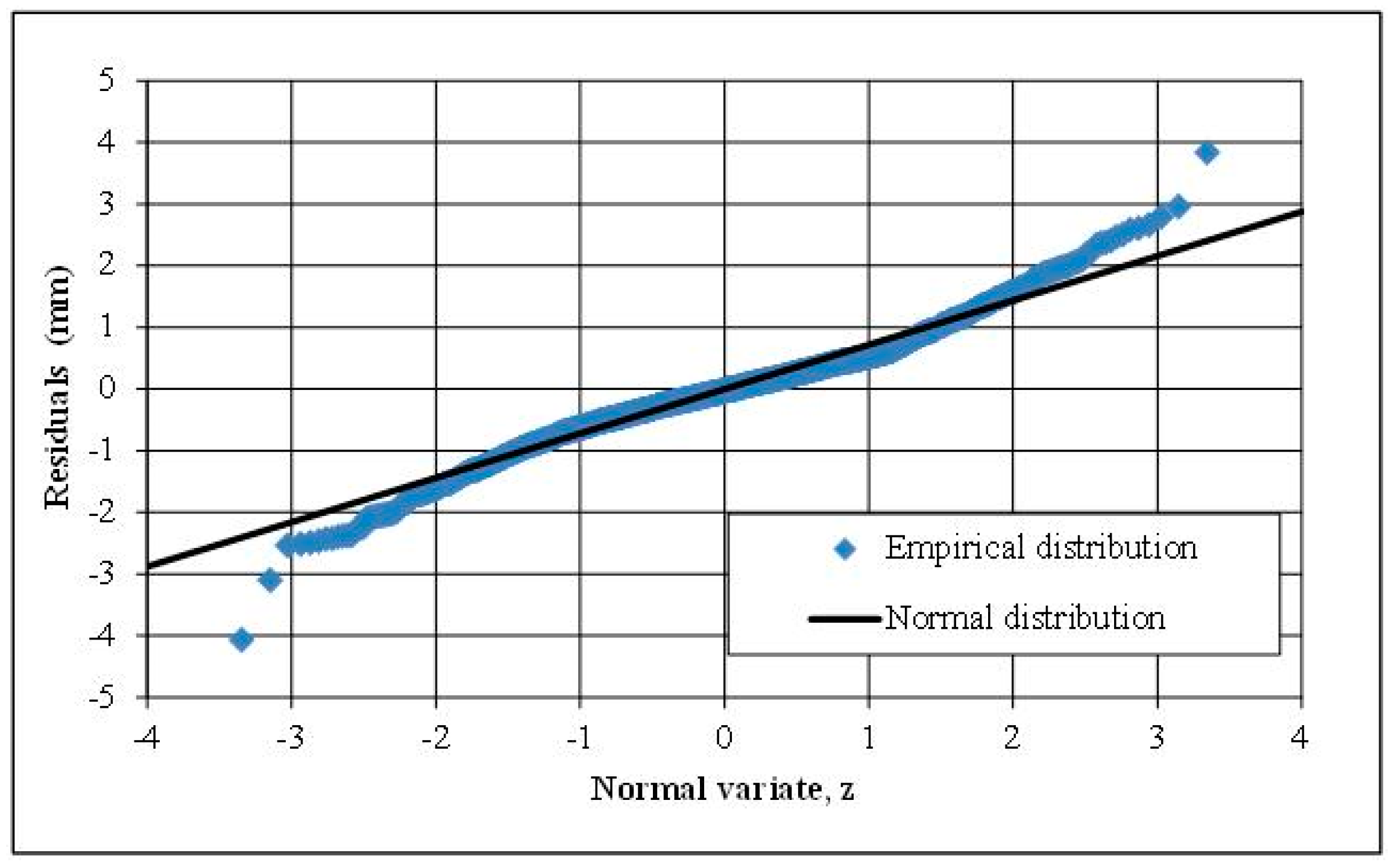
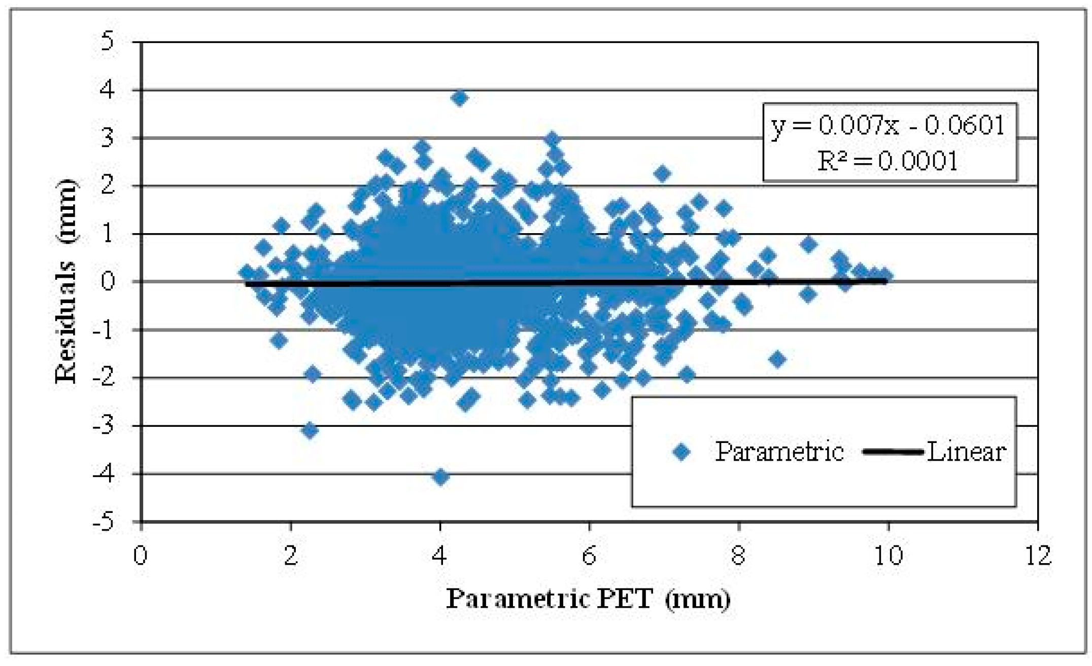
In order to explain the poor performance of the model at the problematic 212 stations shown in Figure 6 (highlighted with blue points), we investigated the model residuals, i.e., the differences between model predictions and PM estimations. As shown in Figure 7, the residuals are approximately normally distributed, while as shown in Figure 8, they are uncorrelated. Therefore, the statistical behavior of the residuals is close to the desirable one (i.e., white noise), indicating absence of systematic errors [51,52]. The negative NSE values are attributed to local overestimation during the warm months or underestimation during the cold months of the year, respectively, driven from the absence of relative humidity and wind speed from the parametric model formulation.

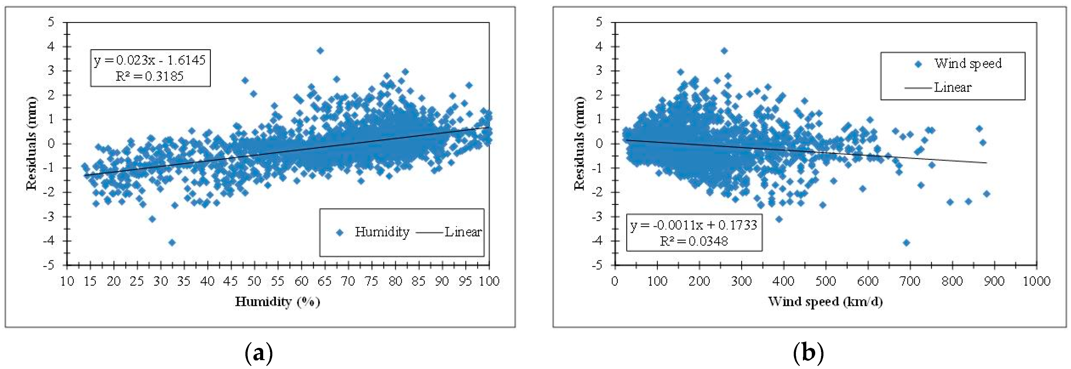
In order to further evaluate the effect of missing information of relative humidity and wind speed on the produced residuals, we plotted both of them along with the corresponding linear models, as presented in Figure 9. This illustrates that there is a significant linear correlation between the relative humidity and the estimation errors—residuals while the opposite seems to be the case for the wind speed. The absence of these two variables as explanatory input variables within the parametric model seem to be crucial in regions with seasonal variations of ET₀ due to energy or water limitations mainly in the tropical zone, as shown in Figure 6.

5.3. Evaluation of Model Performance across Geographical Zones

According to the acquired values of NSE (

Table 4. Number of stations and associated NSE intervals across geographical zones.

Region	1.0–0.9	0.9–0.8	0.8–0.7	0.7–0.6	0.6–0.5	<0.5
Africa	34	16	12	9	7	22
Oceania	67	10	7	4	1	11
Eurasia	68	12	7	4	3	6
N. America	65	15	5	3	2	10
S. America	54	12	10	7	6	11

, Figure 10), the parametric model performs well in Eurasia, North America, and the wider region of Oceania, where 80%, 80%, and 77% of stations, respectively, present efficiency values more than 0.80. In South America, 66% of stations achieve a score greater than 0.80, while in Africa, this percentage falls to 50%. In particular, 22% of stations in Africa achieved NSE values below 0.50, which indicates a poor predictive capacity.

The mean absolute error of the parametric model in every geographical unit is small (

Table 5. Number of stations and associated intervals of monthly MAE across geographical zones.

Region	0–2 mm	2–4 mm	4–6 mm	6–8 mm	8–10 mm	>10 mm
Africa	36	36	15	6	3	4
Oceania	52	36	9	3	0	0
Eurasia	39	37	17	5	1	1
N. America	40	39	17	3	1	0
S. America	69	26	4	1	0	0

). In South America, the MAE of the 95% of the stations is below 4 mm/month. This percentage is 88% for the wider region of Oceania, 79% for North America, 76% for Eurasia, and 72% for Africa.

Table 6. Number of stations and associated intervals of BIAS across geographical zones.

Region	−0.122–0.000	0.000–0.001	0.001–0.062
Africa	65	14	21
Oceania	38	12	50
Eurasia	72	5	23
N. America	68	13	19
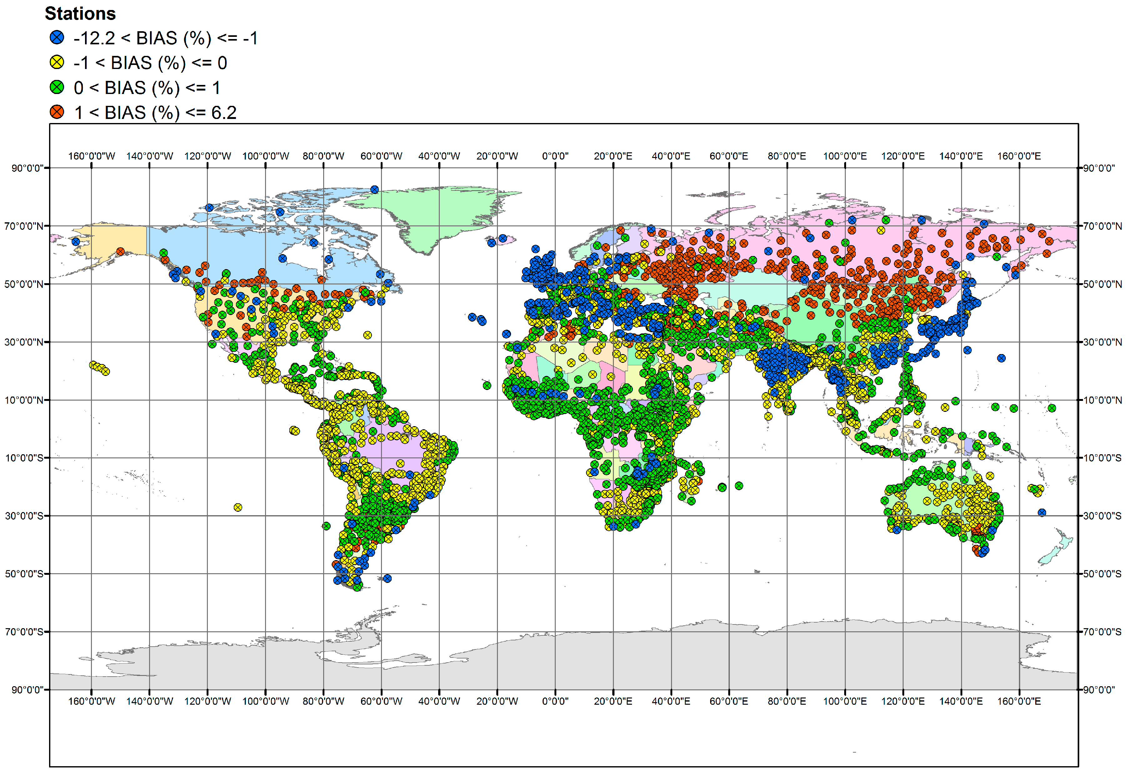
S. America	55	15	30

summarizes the values of the relative bias of the parametric model against the reference PET values, for all of the geographical units (Figure 11). It is obvious that the values are generally small, ranging from –0.122 to +0.062 proving that the results of the parametric model are almost unbiased for the majority of the stations. The differences between the biases across the geographical zones are not important, since the variation between the extreme values is similar.

The overall evaluation of the model across the different geographical areas is very satisfactory. All of the metrics prove that the predictive capacity of the model is very satisfying across Eurasia, North America, and the wider region of Oceania. On the other hand, in the equatorial regions of South America, Africa as well as the Indian and Indonesian Peninsula (Figure 6), the model performs poorly according to the NSE criterion, probably because it does not account for relative humidity and wind speed, which are key drivers of the evapotranspiration processes across these areas, influencing the net incoming solar radiation and the evaporation demand.

6. Spatial Analysis and Model Validation

6.1. Spatial Interpolation of Optimized Parameters

Even though point PET estimates can be used for small-scale studies, it is the regionalisation of PET that is of great significance in hydrological science [53]. A preliminary attempt in PET mapping was presented by Foyster [54], and followed by several publications where different spatial interpolation methods have been applied [55,56,57,58,59], with satisfying performance. In a recent study, Tegos et al. [25] illustrated that the inverse distance method (IDW) was the most efficient than other interpolation techniques, i.e., Kriging, Bilinear Surface Smoothing and Natural Neighbours. Furthermore, IDW is a straightforward and computationally non-intensive method, which is capable to address the huge spatial extent of the study area, i.e., the entire globe.

Formally, the IDW method is used to estimate the unknown value $\widehat{y}\left(S_0\right)$ in location S₀ given the observed y values at sampled locations S_i in the following manner:

$$\widehat{y}\left(S_0\right)={{\displaystyle \sum }}_{i=1}^n{\mathsf{\lambda }}_{i}y\left(S_i\right)$$

(10)

Essentially, the estimated value in S₀ is a linear combination of the weights (λ_i) and observed y values in S_i, where λ_i is defined as:

$${\lambda }_i=\frac{d_{0i}^{–a}}{{{\displaystyle \sum }}_{i=1}^n{d}_{0i}^{–a}}$$

(11)

with:

$${\displaystyle \sum }_{i=1}^n{\mathsf{\lambda }}_i=1$$

(12)

In Equation (10), the numerator is the inverse of distance d_0i between S₀ and S_i with a power α, and the denominator is the sum of all inverse-distance weights for all locations i (in the particular case, all stations exhibiting positive efficiency).

6.2. Spatial Distribution of Parameters

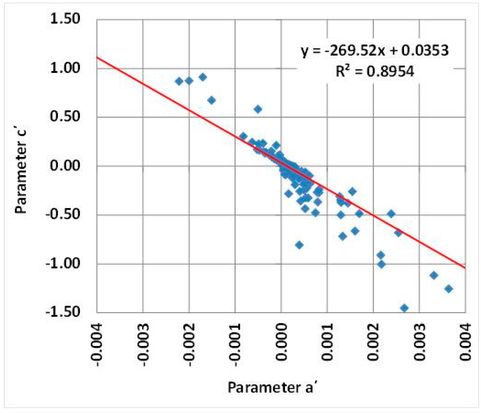
Our approach allows for mapping the spatial distribution of the optimized model parameters a′ and c′, instead of its response, i.e., PET. This is a major advantage, since it allows implementing Equation (5) wherever in the globe, using interpolated values of the point (i.e., locally calibrated) parameters. It is interesting to note that the two parameters are negatively correlated (Figure 12), thus reflecting the significant correlation of the associated meteorological variables of the parametric formula (extraterrestrial radiation, in the numerator, and temperature, in the denominator).

In this context, based on the optimized parameters from the final data set of 4088 stations (as already explained, the rest of stations are not acceptable, and hence the corresponding parameter values will be unreliable), we created maps of spatially-interpolated parameters over the globe. The IDW method was employed in a GIS environment, considering for practical reasons (i.e., in order to avoid extreme computational burden), a relatively large grid size of 0.1 decimal degrees in WGS84 coordinate system and a variable search radius including the 12 nearest stations, in order to tackle the measurement of large distances across the globe.

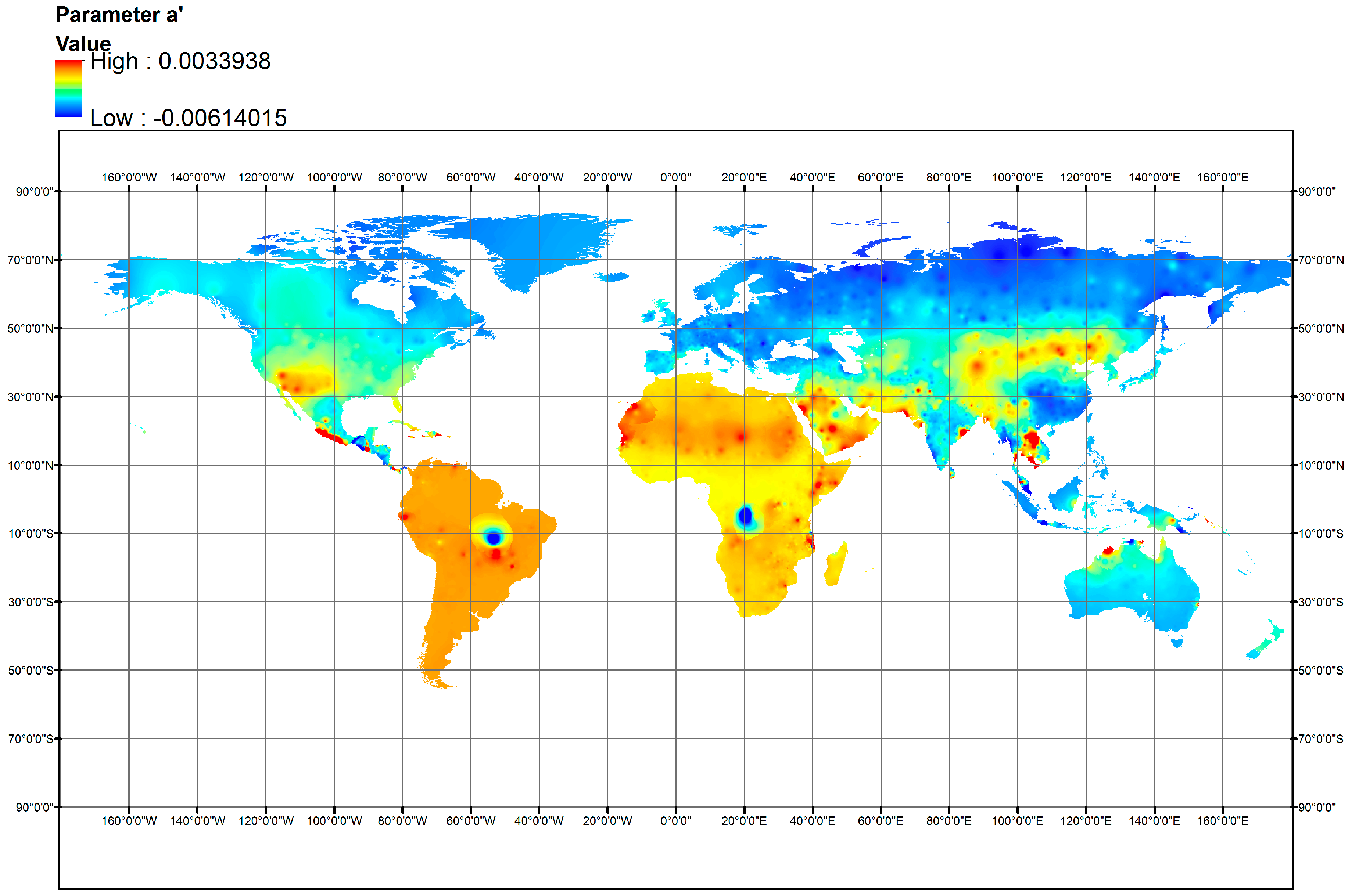
Figure 13 illustrates the spatial distribution of parameter a′. The highest values are generally observed around the equatorial zone, while they are getting lower as we move away from it. This is a reasonable outcome since this parameter is associated with solar radiation. This means that around the equatorial zone, where the incoming solar radiation is higher, the values of parameter a′ are to be higher while around the poles, where solar radiation is lower, the values of parameter a′ were expected to be lower. Another observation is that in the case of two stations, one located at Brazil and one at the Democratic Republic of Congo, the calculated values for parameter a′ were low, creating “sinkholes” in the corresponding maps. This is explained from the fact that at those areas, the hydro-meteorological network is not dense enough, thus the influence of the specific stations extends, as a direct effect of the IDW implementation. Apart from this, the spatial analysis of parameter a′ is normal and physically explained.

In contrast to parameter a′, the spatial distribution of parameter c′, depicted in Figure 14, the lowest values around the equatorial zone, while these are getting higher as we move away from the equator. Since c′ is inversely proportional to temperature, it was expected that its values get higher as temperature is getting lower and vice versa. In the case of the above stations, i.e., one at Brazil and one at the Democratic Republic of Congo, the values of parameter c′ were extremely high, contrariwise to parameter a′. The explanation for this phenomenon is the same as above, yet in this case the interpolation method resulted in a ridge-type distribution over the specific areas.

Conclusively, the model results can be considered reliable, since the spatial distribution of both parameters around the globe is physically explained, while minor irregularities are also attributed to physical reasons, i.e., inadequate representation of humidity and wind processes.

6.3. Model Validation

The validation of the model was performed by comparing monthly ET₀ predictions provided by the parametric formula (Equation (5)), using interpolated parameters against PM estimates in a number of independent stations. In particular, we considered two validations sets, a “local” and a “global” one. The former comprises 37 stations across California, for which monthly meteorological time series are available from the California Irrigation Management Information System [60]. The “global” set comprises 17 stations from countries with different hydroclimatic regimes (Spain, Germany, Ireland, Greece, Iran, and Australia), for which we obtained full time series of the required meteorological data, at the monthly scale, form various data sources.

For the local validation set (

Table 7. Statistical indices for the local validation dataset (CIMIS stations, California, USA).

a/a	Station	Validation Period	NSE	MAE (mm)	BIAS
1	Five Points	June 1982–June 2013	0.880	20.4	−0.09
2	Davis	October 1982–June 2013	0.857	13.8	−0.01
3	Firebaugh/Telles	October 1982–June 2013	0.897	16.8	−0.09
4	Gerber	October 1982–June 2013	0.896	17.9	−0.10
5	Durham	October 1982–June 2013	0.870	19.7	−0.14
6	Carmino	November 1982–June 2013	0.952	11.3	−0.01
7	Stratford	November 1982–June 2013	0.913	17.2	−0.06
8	Castroville	December 1982–June 2013	0.442	23.7	−0.23
9	Kettleman	December 1982–June 2013	0.903	18.8	−0.10
10	Bishop	March 1983–June 2013	0.475	16.5	0.03
11	Parlier	June 1983–June 2013	0.858	22.1	−0.16
12	McArthur	December 1983–June 2013	0.940	11.5	0.01
13	U.C. Riverside	June 1985–June 2013	0.858	13.2	0.08
14	Brentwood	May 1986–October 2006	0.930	13.2	−0.06
15	San Luis Obispo	May 1986–June 2013	0.856	12.0	−0.08
16	Blackwells corner	May 1987–June 2013	0.939	13.7	−0.05
17	Los Banos	June 1988–June 2013	0.926	14.0	−0.06
18	Buntingville	May 1986–June 2013	0.953	11.1	0.03
19	Temecula	December 1986–June 2013	0.769	12.9	0.02
20	Santa Ynez	December 1986–June 2013	0.842	13.6	−0.10
21	Seeley	June 1987–June 2013	0.845	18.4	0.03
22	Manteca	December 1987–June 2013	0.796	25.2	−0.10
23	Modesto	October 1987–June 2013	0.922	14.7	−0.06
24	Irvine	November 1987–June 2013	0.803	13.2	−0.10
25	Oakville	October 1989–June 2013	0.930	13.3	−0.10
26	Pomona	April 1989–June 2013	0.701	19.0	−0.15
27	Fresno State	November 1988–June 2013	0.906	18.4	−0.12
28	Santa Rosa	January 1990–June 2013	0.894	11.5	−0.09
29	Browns Valley	May 1989–June 2013	0.856	22.3	−0.16
30	Lindcove	June 1989–June 2013	0.782	31.0	−0.22
31	Alturas	May 1989–June 2013	0.916	10.4	−0.02
32	Cuyama	October 1989–June 2013	0.950	11.5	0.05
33	Tulelake FS	May 1989–June 2013	0.922	11.9	0.05
34	Windsor	January 1991–June 2013	0.905	11.4	−0.09
35	De Laveaga	October 1990–June 2013	0.676	21.8	−0.19
36	Westlands	May 1992–June 2013	0.932	15.0	−0.03
37	Sanel Valley	February 1991–June 2013	0.939	11.0	−0.02
Average			0.855	16.0	−0.07

), the model predicts monthly ET₀ with significant accuracy, thus exhibiting an average efficiency up to 0.855, and an average bias of only −0.07. Except for three stations (Bishop, Castroville, De Laveaga), the NSE exceeds 0.70, while in 17 out of 37 stations it exceeds 0.90. This indicates an almost perfect performance, particularly when taking into account that the model has been calibrated using abstract (i.e., mean monthly) meteorological information over the entire globe, while the validation set comprises detailed data, both in terms of spatial extent and temporal resolution. Similarly satisfying are the outcomes from the global validation set, which are summarized in

Table 8. Statistical indexes for the global validation dataset.

a/a	Station	Country	Validation Period	NSE	MAE (mm)	BIAS
1	Aachen	Germany	January 1951–May 2011	0.955	6.8	0.06
2	Bremen	Germany	January 1951–May 2011	0.954	5.5	0.03
3	Alicante	Spain	January 1980–September 2010	0.916	11.1	0.00
4	Badajoz	Spain	January 1961–May 2005	0.921	13.0	−0.09
5	Valencia	Spain	September 1954–August 1964	0.893	10.0	−0.06
6	Zaragoza	Spain	February 1974–January 1996	0.953	10.8	−0.01
7	Herakleion	Greece	January 1968–December 1989	0.947	10.2	−0.00
8	Kerkyra	Greece	January 1968–December 1989	0.936	9.8	−0.09
9	Kavala	Greece	January 1968–December 1989	0.835	13.5	0.04
10	Limnos	Greece	January 1968–December 1989	0.762	24.3	0.12
11	Athens	Greece	January 1968–December 1989	0.924	13.6	0.03
12	Melbourne	Australia	January 2009–January 2016	0.752	18.5	0.17
13	Dublin	Ireland	January 2013–June 2016	0.870	5.1	−0.09
14	Bandar-Anzali	Iran	January 1990–December 2005	0.875	13.9	−0.16
15	Ramsar	Iran	January 1990–December 2005	0.788	16.2	0.15
16	Khorram-Abad	Iran	January 1990–December 2005	0.400	38.3	0.37
17	Kashan	Iran	January 1990–December 2005	0.804	19.6	−0.13
Average				0.852	14.1	0.02

(average efficiency 0.852, average bias 0.02), thus confirming the model predictive capacity across different climates.

7. Conclusions

In the present study, the concept of parametric PET modelling was thoroughly analyzed, by performing a global survey of its applicability. The model has a very simple structure and uses easily retrieved information, by means of air temperature and extraterrestrial radiation. Therefore, the model is simultaneously simple and parsimonious, in terms of both parameterization and data requirements.

Preliminary analysis of the extended climatic data at 4300 stations worldwide, provided by the FAO CLIMWAT database, allowed for justifying the use of temperature and extraterrestrial radiation as key explanatory variables of reference PET over the globe. However, it also indicated that in few cases the two variables exhibit irregular seasonal patterns, which cannot be adequately represented through simple modelling structures. The statistical analysis of the residuals, in these cases, showed that the model is consistent in terms of parameters estimation and model validation.

At all CLIMWAT stations, we provided optimal estimations of model parameters c′ and a′, by calibrating them against given Penman-Monteith values at the mean monthly scale. Using typical goodness-of-fitting criteria (efficiency, mean absolute error, relative bias), we evaluated the model performance, which was generally very satisfying in a large portion of stations. However, in less than 10% of the data set the calibrated model exhibited negative efficiency. Further analysis across broader geographical regions showed that the model deviates from the Penman-Monteith PET estimates in some locations, which is rather expected due to the significant influence of relative humidity and wind speed, which are not accounted for in the parametric model.

An important outcome of this research was the generation of spatially distributed maps of model parameters, by employing the IDW interpolation technique against their optimized values at 4088 out of 4300 stations, exhibiting non-negative efficiency (the dataset of point parameter estimations is available at http://www.itia.ntua.gr/en/docinfo/1738/). The spatial pattern of both parameters over the globe is fully reasonable, which is a strong indicator of their physical consistency. These maps can be straightforwardly used to provide suitable parameter values at both the local and regional scale, thus allowing for the direct use of the parametric model wherever in the world.

The validation procedure against PM estimates from detailed meteorological information (i.e., monthly time series) from 37 stations across California, as well as 17 independent stations across Europe, Asia, and Australia, proved that the application of the parametric model using spatially interpolated parameters provides reliable estimates, thus being a promising alternative of the widely recognized yet data demanding Penman-Monteith approach, when there is lack of the full data set that the latter requires.

Future research steps include a detailed investigation of the factors affecting the model poor performance in specific areas over the globe, in order to recognize whether these can be handled through a slightly different model structure or they do require the use of additional explanatory variables or parameters. Apparently, this will require the use of full meteorological time series instead of climatic data, which is a very challenging task at global scale. A survey of the calibration results against different climatic zones is another challenging task that will further highlight the model advantages, as well as potential shortcomings.

References

- Koutsoyiannis, D.; Mamassis, N.; Tegos, A. Logical and illogical exegeses of hydrometeorological phenomena in ancient Greece. Water Sci. Technol. Water Supply 2007, 7, 13–22. [Google Scholar] [CrossRef]
- McMahon, T.A.; Peel, M.C.; Lowe, L.; Srikanthan, R.; McVicar, T.R. Estimating actual, potential, reference crop and pan evaporation using standard meteorological data: A pragmatic synthesis. Hydrol. Earth Syst. Sci. 2013, 17, 1331–1363. [Google Scholar] [CrossRef]
- McMahon, T.A.; Finlayson, B.L.; Peel, M.C. Historical developments of models for estimating evaporation using standard meteorological data. Wiley Interdiscip. Rev. Water 2016, 3, 788–818. [Google Scholar] [CrossRef]
- Dingman, S.L. Physical Hydrology; MacMillan Publishing Company: New York, NY, USA, 1994. [Google Scholar]
- Doorenbos, J.; Pruitt, W.O. Guidelines for Predicting Crop Water Requirements: Rome, Italy, Food and Agricultural Organization of the United Nations. FAO Irrigation and Drainage Paper 24. 1977. Available online: http://www.fao.org/3/a-f2430e.pdf (accessed on 13 October 2017).
- Allen, R.G.; Jensen, M.E.; Wright, J.L.; Burman, R.D. Operational estimates of reference evapotranspiration. Agron. J. 1989, 81, 650. [Google Scholar] [CrossRef]
- Xu, C.-Y.; Singh, V.P. Evaluation and generalization of temperature-based methods for calculating evaporation. Hydrol. Process. 2001, 15, 305–319. [Google Scholar] [CrossRef]
- Allen, R.G.; Pruitt, W.O. Rational use of the FAO Blaney-Criddle formula. J. Irrig. Drain. Eng. 1986, 112, 139–155. [Google Scholar] [CrossRef]
- Amatya, D.M.; Skaggs, R.W.; Gregory, J.D. Comparison of methods for estimating REF-ET. J. Irrig. Drain. Eng. 1995, 121, 427–435. [Google Scholar] [CrossRef]
- Mohawesh, O.E. Spatio-temporal calibration of Blaney–Criddle equation in arid and semiarid environment. Water Resour. Manag. 2010, 24, 2187–2201. [Google Scholar] [CrossRef]
- Sentelhas, P.C.; Gillespie, T.J.; Santos, E.A. Evaluation of FAO Penman-Monteith and alternative methods for estimating reference evapotranspiration with missing data in Southern Ontario, Canada. Agric. Water Manag. 2010, 97, 635–644. [Google Scholar] [CrossRef]
- Oudin, L.; Hervieu, F.; Michel, C.; Perrin, C.; Andréassian, V.; Anctil, F.; Loumagne, C. Which potential evapotranspiration input for a lumped rainfall–runoff model? Part 2—Towards a simple and efficient potential evapotranspiration model for rainfall–runoff modelling. J. Hydrol. 2005, 303, 290–306. [Google Scholar] [CrossRef]
- Gavilán, P.; Lorite, I.J.; Tornero, S.; Berengena, J. Regional calibration of Hargreaves equation for estimating reference ET in a semiarid environment. Agric. Water Manag. 2006, 81, 257–281. [Google Scholar] [CrossRef]
- Fooladmand, H.R.; Haghighat, M. Spatial and temporal calibration of Hargreaves equation for calculating monthly ET0 based on Penman-Monteith method. Irrig. Drain. 2007, 56, 439–449. [Google Scholar] [CrossRef]
- Tabari, H.; Talaee, P.H. Local calibration of the Hargreaves and Priestley-Taylor equations for estimating reference evapotranspiration in arid and cold climates of Iran based on the Penman-Monteith model. J. Hydrol. Eng. 2011, 16, 837–845. [Google Scholar] [CrossRef]
- Hu, Q.F.; Yang, D.W.; Wang, Y.T.; Yang, H.B. Global calibration of Hargreaves equation and its applicability in China. Adv. Water Sci. 2011, 22, 160–167. [Google Scholar]
- Haslinger, K.; Bartsch, A. Creating long-term gridded fields of reference evapotranspiration in Alpine terrain based on a recalibrated Hargreaves method. Hydrol. Earth Sys. Sci. 2016, 20, 1211–1223. [Google Scholar] [CrossRef]
- Choudhury, B.J. Global pattern of potential evaporation calculated from the Penman-Monteith equation using satellite and assimilated data. Remote Sens. Environ. 1997, 61, 64–81. [Google Scholar] [CrossRef]
- Allen, R.G.; Tasumi, M.; Trezza, R. Satellite-based energy balance for mapping evapotranspiration with internalized calibration (METRIC)-Model. J. Irrig. Drain. Eng. 2007, 133, 380–394. [Google Scholar] [CrossRef]
- Allen, R.; Irmak, A.; Trezza, R.; Hendrickx, J.M.; Bastiaanssen, W.; Kjaersgaard, J. Satellite-based ET estimation in agriculture using SEBAL and METRIC. Hydrol. Process. 2011, 25, 4011–4027. [Google Scholar] [CrossRef]
- Mu, Q.; Heinsch, F.A.; Zhao, M.; Running, S.W. Development of a global evapotranspiration algorithm based on MODIS and global meteorology data. Remote Sens. Environ. 2007, 111, 519–536. [Google Scholar] [CrossRef]
- Mu, Q.; Zhao, M.; Running, S.W. Improvements to a MODIS global terrestrial evapotranspiration algorithm. Remote Sens. Environ. 2011, 115, 1781–1800. [Google Scholar] [CrossRef]
- Vinukollu, R.K.; Wood, E.F.; Ferguson, C.R.; Fisher, J.B. Global estimates of evapotranspiration for climate studies using multi-sensor remote sensing data: Evaluation of three process-based approaches. Remote Sens. Environ. 2011, 115, 801–823. [Google Scholar] [CrossRef]
- Tegos, A.; Efstratiadis, A.; Koutsoyiannis, D. A parametric model for potential evapotranspiration estimation based on a simplified formulation of the Penman-Monteith equation. In Evapotranspiration—An Overview; InTech: Rijeka, Croatia, 2013; pp. 143–165. [Google Scholar]
- Tegos, A.; Malamos, N.; Koutsoyiannis, D. A parsimonious regional parametric evapotranspiration model based on a simplification of the Penman-Monteith formula. J. Hydrol. 2015, 524, 708–717. [Google Scholar] [CrossRef]
- Hargreaves, G.H.; Samani, Z.A. Reference crop evaporation from temperature. Appl. Eng. Agric. 1985, 1, 96–99. [Google Scholar] [CrossRef]
- Jensen, M.E.; Haise, H.R. Estimating evapotranspiration from solar radiation. J. Irrig. Drain. Div. Proc. 1963, 89, 15–41. [Google Scholar]
- McGuinness, J.L.; Bordne, E.F. A Comparison of Lysimeter-Derived Potential Evapotranspiration with Computed Values; US Department of Agriculture: Washington, DC, USA, 1972.
- Malamos, N.; Tegos, A.; Tsirogiannis, I.L.; Christofides, A.; Koutsoyiannis, D. Implementation of a regional parametric model for potential evapotranspiration assessment. In Proceedings of the IrriMed 2015—Modern Technologies, Strategies and Tools for Sustainable Irrigation Management and Governance in Mediterranean Agriculture, Bari, Italy, 23–25 September 2015. [Google Scholar]
- Allen, R.G.; Pereira, L.S.; Raes, D.; Smith, M. Crop Evapotranspiration-Guidelines for Computing Crop Water Requirements—FAO Irrigation and Drainage Paper 56; FAO: Rome, Italy, 1998; pp. 377–384. [Google Scholar]
- Ward, W.C.; Robinson, M. Principles of Hydrology; McGraw-Hill: New York, NY, USA, 1990. [Google Scholar]
- Koutsoyiannis, D.; Xanthopoulos, T. Engineering Hydrology, 3rd ed.; National Technical University of Athens: Athens, Greece, 1999; p. 418. (In Greek) [Google Scholar]
- Tegos, A.; Efstratiadis, A.; Malamos, N.; Mamassis, N.; Koutsoyiannis, D. Evaluation of a parametric approach for estimating potential evapotranspiration across different climates. Agric. Agric. Sci. Procedia 2015, 4, 2–9. [Google Scholar] [CrossRef]
- Tegos, A.; Mamassis, N.; Koutsoyiannis, D. Estimation of Potential Evapotranspiration with Minimal Data Dependence. EGU General Assembly Conference Abstracts, Volume 11, 1937, European Geosciences Union, 2009. Available online: http://www.itia.ntua.gr/en/docinfo/905/ (accessed on 16 October 2017).
- Tegos, A.; Tyralis, H.; Koutsoyiannis, D.; Hamed, K. An R function for the estimation of trend significance under the scaling hypothesis-application in PET parametric annual time series. Open Water J. 2017, 4, 6. [Google Scholar]
- Koutsoyiannis, D. Hydrology and Change. Hydrol. Sci. J. 2013, 58, 1177–1197. [Google Scholar] [CrossRef]
- Efstratiadis, A.; Koutsoyiannis, D. One decade of multiobjective calibration approaches in hydrological modelling: A review. Hydrol. Sci. J. 2010, 55, 58–78. [Google Scholar] [CrossRef]
- Priestley, C.H.B.; Taylor, R.J. On the assessment of surface heat fluxes and evaporation using large-scale parameters. Mon. Weather Rev. 1972, 100, 81–92. [Google Scholar] [CrossRef]
- Food and Agriculture Organization of the United Nations (FAO). CLIMWAT for CROPWAT, A Climatic Database for Irrigation Planning and Management. FAO Irrigation & Drainage Paper No. 49, Rome. 1993. Available online: http://www.fao.org/nr/water/infores_databases_climwat.html (accessed on 16 October 2017).
- Lofgren, B.M.; Hunter, T.S.; Wilbarger, J. Effects of using air temperature as a proxy for evapotranspiration in climate change scenarios of Great Lakes basin hydrology. J. Gt. Lakes Res. 2011, 37, 744–752. [Google Scholar] [CrossRef]
- McVicar, T.R.; Roderick, M.L.; Donohue, R.J.; Li, L.T.; Van Niel, T.G.; Thomas, A.; Grieser, J.; Jhajharia, D.; Himri, Y.; Mahowald, N.M.; et al. Global review and synthesis of trends in observed terrestrial near-surface wind speeds: Implications for evaporation. J. Hydrol. 2012, 416–417, 182–205. [Google Scholar] [CrossRef]
- Guo, D.; Westra, S.; Maier, H.R. Sensitivity of potential evapotranspiration to changes in climate variables for different climatic zones. Hydrol. Earth Syst. Sci. 2016, 1–43. [Google Scholar] [CrossRef]
- Rayner, D.P. Wind run changes: The dominant factor affecting pan evaporation trends in Australia. J. Clim. 2017, 20, 3379–3394. [Google Scholar] [CrossRef]
- Roderick, M.L.; Rotstayn, L.D.; Farquhar, G.D.; Hobbins, M.T. On the attribution of changing pan evaporation. Geophys. Res. Lett. 2007, 34, 251–270. [Google Scholar] [CrossRef]
- Roderick, M.L.; Hobbins, M.T.; Farquhar, G.D. Pan evaporation trends and the terrestrial water balance. II. Energy balance and interpretation. Geogr. Compass 2009, 3, 761–780. [Google Scholar] [CrossRef]
- Wang, W.; Shao, Q.; Peng, S.; Xing, W.; Yang, T.; Luo, Y.; Xu, J. Reference evapotranspiration change and the causes across the Yellow River Basin during 1957–2008 and their spatial and seasonal differences. Water Resour. Res. 2012, 48, 113–122. [Google Scholar] [CrossRef]
- Li, Z.; Chen, Y.; Shen, Y.; Liu, Y.; Zhang, S. Analysis of changing pan evaporation in the arid region of Northwest China. Water Resour. Res. 2013, 49, 2205–2212. [Google Scholar] [CrossRef]
- Pereira, L.S.; Allen, R.G.; Smith, M.; Raes, D. Crop evapotranspiration estimation with FAO56: Past and future. Agric. Water Manag. 2015, 147, 4–20. [Google Scholar] [CrossRef]
- Efstratiadis, A.; Koutsoyiannis, D. An evolutionary annealing-simplex algorithm for global optimisation of water resource systems. In Hydroinformatics 2002: Proceedings of the Fifth International Conference on Hydroinformatics, Cardiff, UK, 1–5 July 2002; International Water Association: London, UK, 2002; pp. 1423–1428. [Google Scholar]
- Tsoukalas, I.; Kossieris, P.; Efstratiadis, A.; Makropoulos, C. Surrogate-enhanced evolutionary annealing simplex algorithm for effective and efficient optimization of water resources problems on a budget. Environ. Model. Softw. 2016, 77, 122–142. [Google Scholar] [CrossRef]
- Kitanidis, P.K. Introduction to Geostatistics: Applications in Hydrogeology; Cambridge University Press: New York, NY, USA, 1997. [Google Scholar]
- Malamos, N.; Koutsoyiannis, D. Broken line smoothing for data series interpolation by incorporating an explanatory variable with denser observations: Application to soil-water and rainfall data. Hydrol. Sci. J. 2015, 60, 468–481. [Google Scholar] [CrossRef]
- Merz, R.; Blöschl, G. Regionalisation of catchment model parameters. J. Hydrol. 2004, 287, 95–123. [Google Scholar] [CrossRef]
- Foyster, A.M. Application of the grid square technique to mapping of evapotranspiration. J. Hydrol. 1973, 19, 205–226. [Google Scholar] [CrossRef]
- Dalezios, N.R.; Loukas, A.; Bampzelis, D. Spatial variability of reference evapotranspiration in Greece. Phys. Chem. Earth Parts A/B/C 2002, 27, 1031–1038. [Google Scholar] [CrossRef]
- Mardikis, M.G.; Kalivas, D.P.; Kollias, V.J. Comparison of interpolation methods for the prediction of reference evapotranspiration—An application in Greece. Water Resour. Manag. 2005, 19, 251–278. [Google Scholar] [CrossRef]
- Vicente-Serrano, S.M.; Lanjeri, S.; López-Moreno, J.I. Comparison of different procedures to map reference evapotranspiration using geographical information systems and regression-based techniques. Int. J. Climatol. 2007, 27, 1103–1118. [Google Scholar] [CrossRef] [Green Version]
- Mancosu, N.; Snyder, R.L.; Spano, D. Procedures to develop a standardized reference evapotranspiration zone map. J. Irrig. Drain. Eng. 2014, 140, A4014004. [Google Scholar] [CrossRef]
- Malamos, N.; Tsirogiannis, I.L.; Tegos, A.; Efstratiadis, A.; Koutsoyiannis, D. Spatial interpolation of potential evapotranspiration for precision irrigation purposes. In Proceedings of the 10th World Congress on Water Resources and Environment, Athens, Greece, 5–9 July 2017. [Google Scholar]
- Hart, Q.J.; Brugnach, M.; Temesgen, B.; Rueda, C.; Ustin, S.L.; Frame, K. Daily reference evapotranspiration for California using satellite imagery and weather station measurement interpolation. Civ. Eng. Environ. Syst. 2009, 26, 19–33. [Google Scholar] [CrossRef]
Figure 1.
Food and Agriculture Organization (FAO CLIMWAT) hydrometeorological network (dark areas indicate high altitudes).
Figure 2.
Scatter plot of mean annuals of (a) solar radiation, (b) temperature, (c) relative humidity, (d) wind speed, (e) sunshine duration, (f) extraterrestrial radiation vs. mean annual ET0.
Figure 3.
Scatter plots of monthly extraterrestrial radiation, Ra, vs. mean monthly ET0 (a) and mean monthly temperature, T, vs. ET0 (b) at five stations in Australia, exhibiting loop-type patterns.
Figure 4.
Scatter plots of monthly extraterrestrial radiation, Ra, vs. mean monthly ET0 (a) and mean monthly temperature, T, vs. ET0 (b) at five stations in Australia, exhibiting irregular patterns.
Figure 5.
Ranges of coefficient of determination for the linear regression functions of monthly reference PET against Ra and T, and the nonlinear parametric model.
Figure 6.
CLIMWAT stations with negative NSE.
Figure 7.
Normal probability plot of the empirical distribution function of the mode residuals using Weibull plotting positions against normal distribution function N (0, 0.7), for stations with negative NSE.
Figure 8.
Residuals vs. parametric PET for stations with negative NSE.
Figure 9.
Residuals vs. humidity (a) and wind speed (b) for stations with negative NSE.
Figure 10.
Distribution of NSE across CLIMWAT stations.
Figure 11.
Distribution of BIAS across CLIMWAT stations.
Figure 12.
Scatter plot of optimized parameters through the final data sample of 4088 stations exhibiting positive NSE values.
Figure 13.
Spatial distribution of parameter a′ over the globe.
Figure 14.
Spatial distribution of parameter c′ over the globe.