Modeling Water Yield: Assessing the Role of Site and Region-Specific Attributes in Determining Model Performance of the InVEST Seasonal Water Yield Model

 , , , ,
Abstract
:1. Introduction
2. Materials and Methods
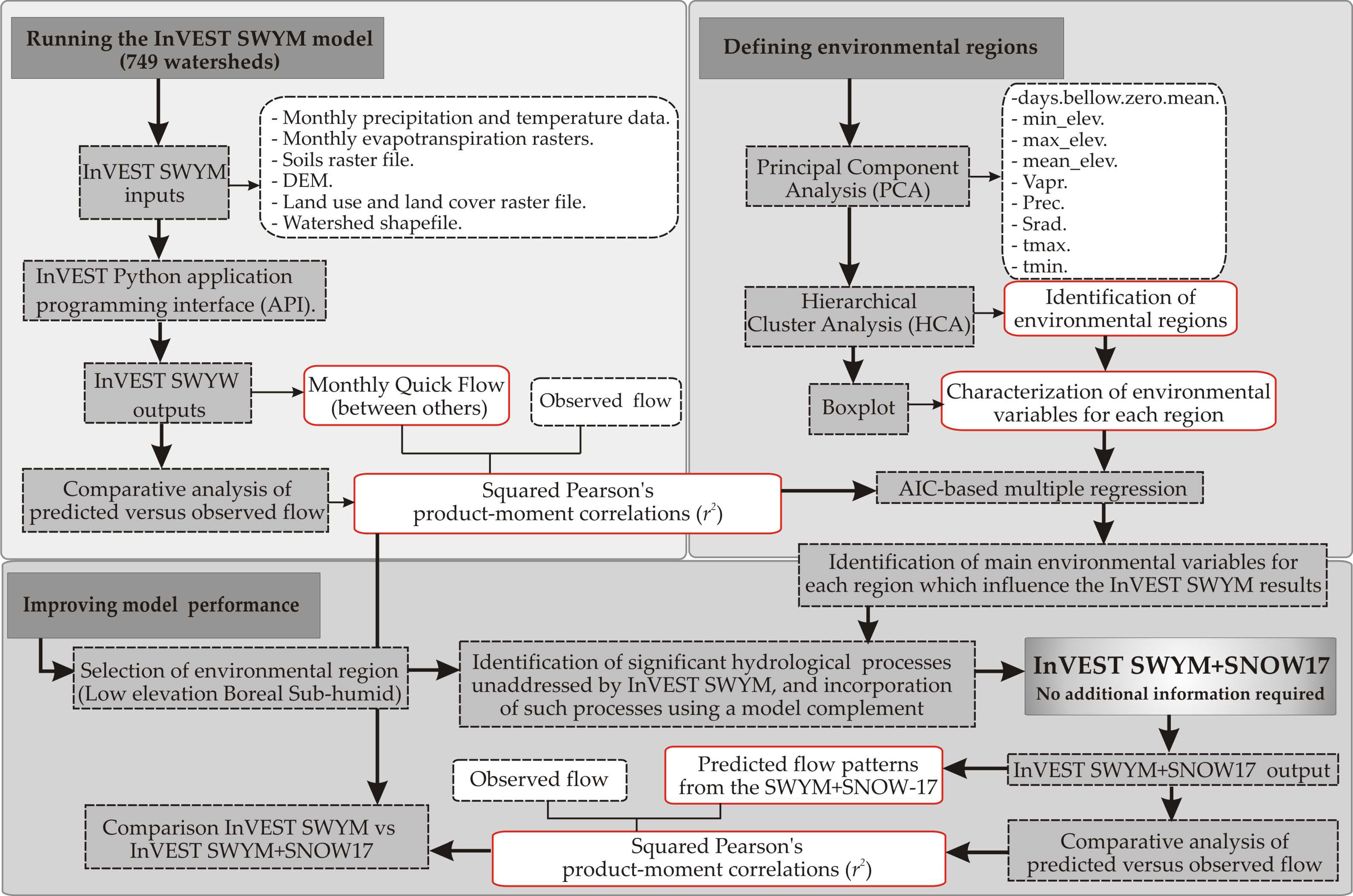
2.1. Running the InVEST Model
2.2. InVEST Model Output
2.3. Comparative Analysis of Predicted versus Observed Flow
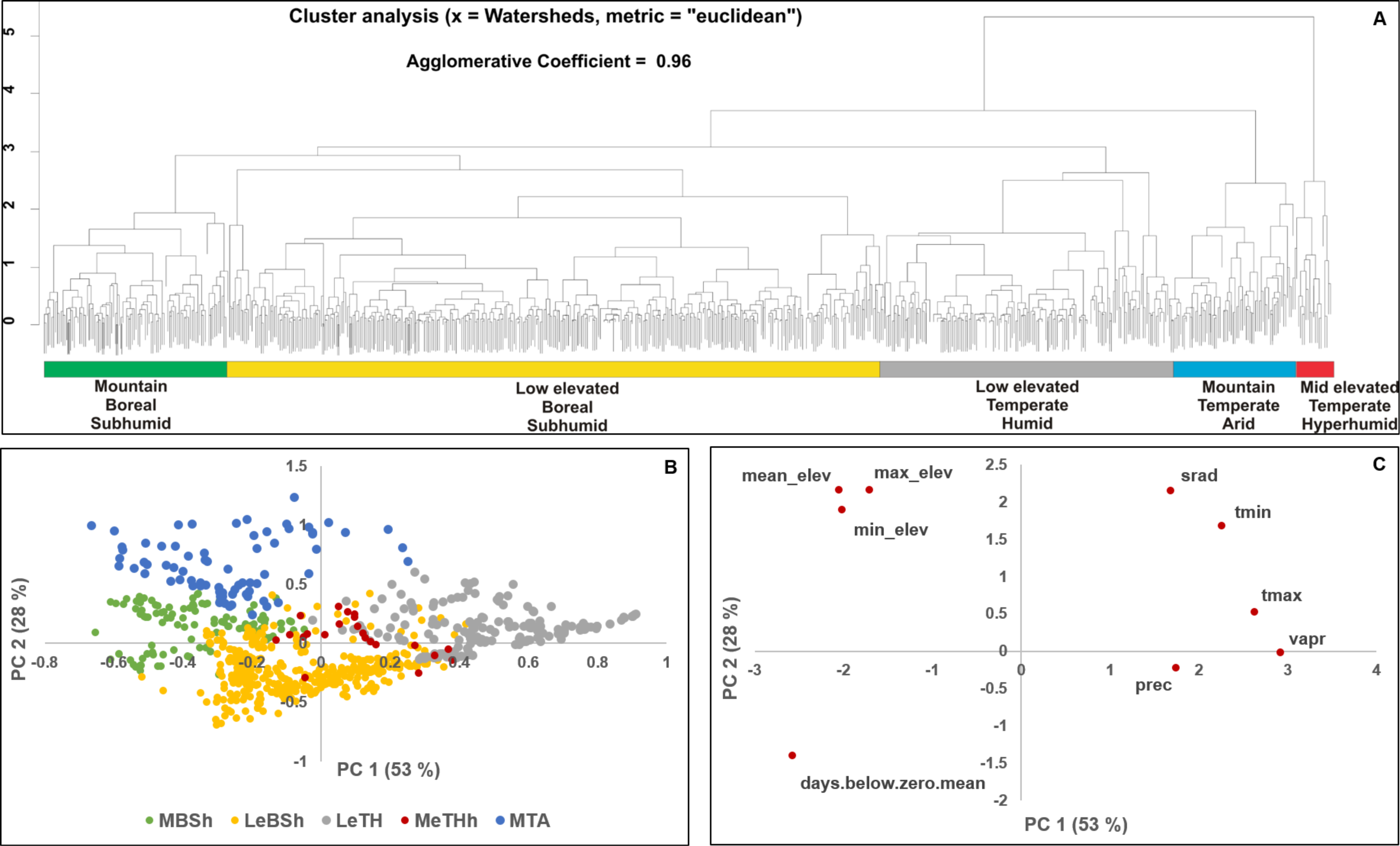
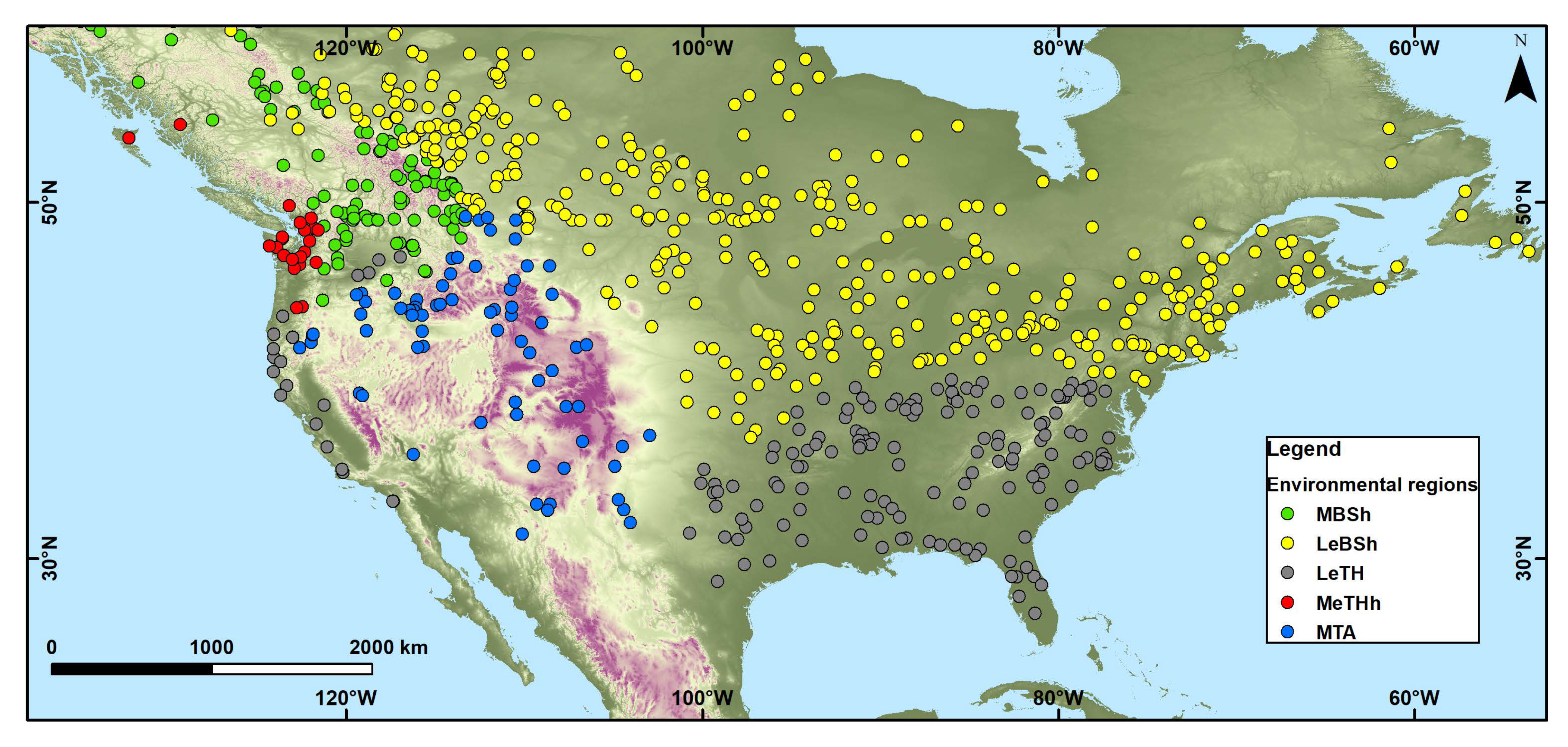
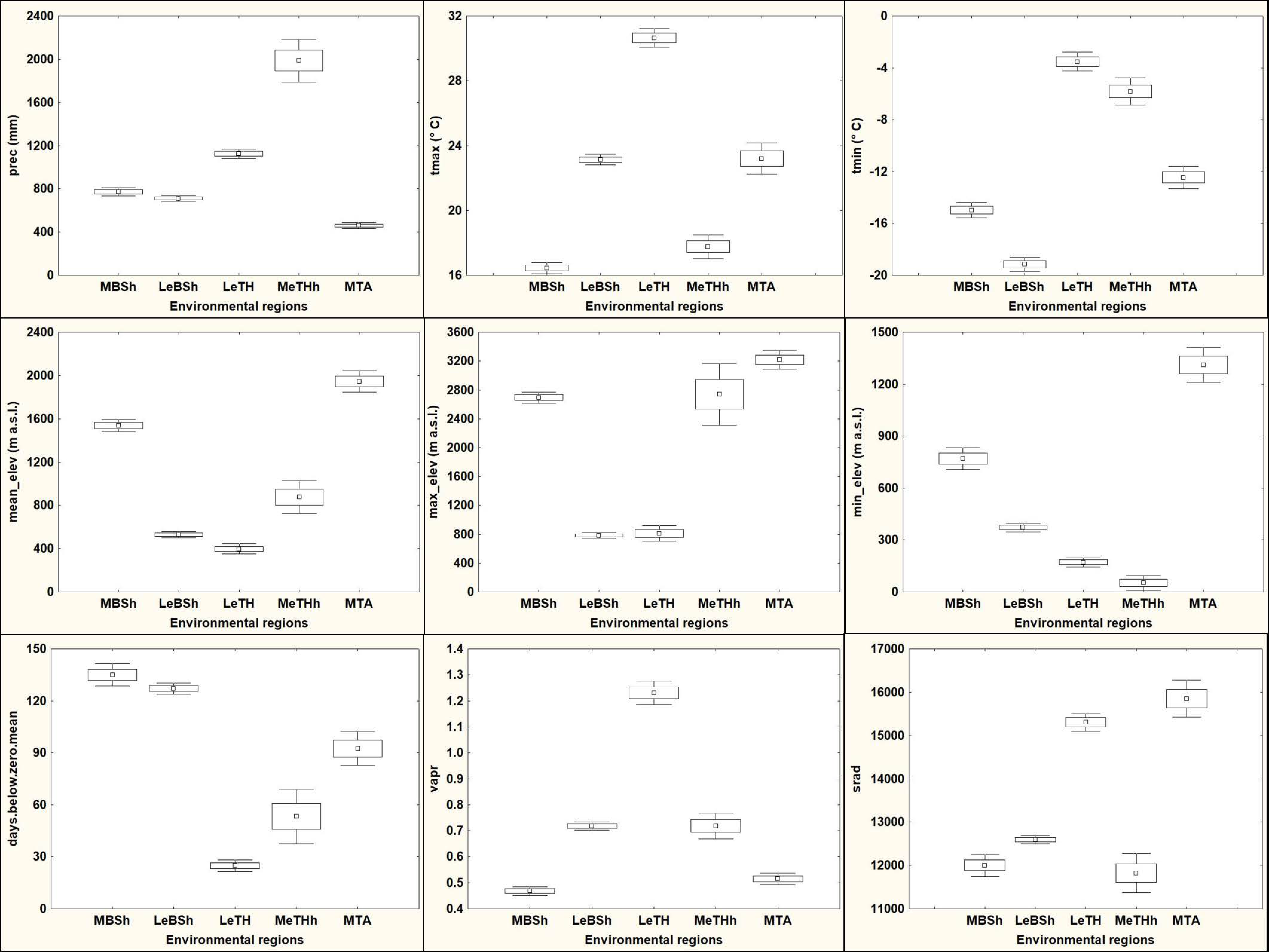
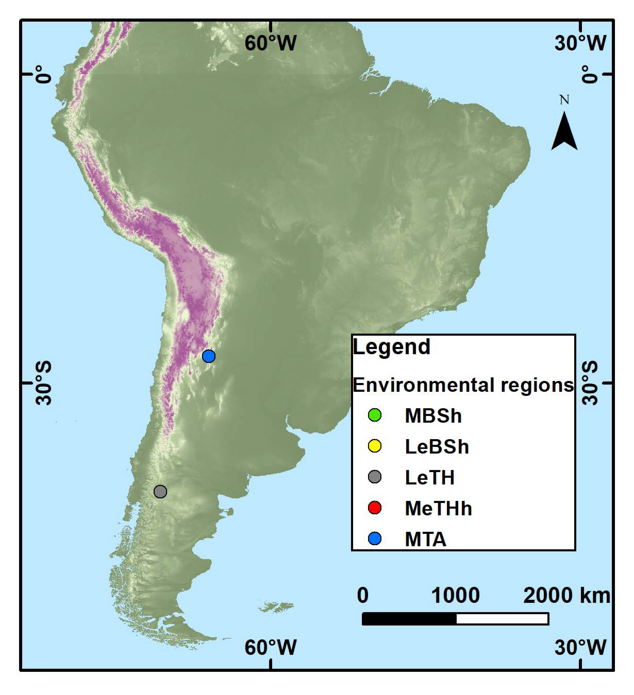
2.4. Defining Regions and Characterization of Climate Variables for Each Region
2.5. Improving Model Performance
3. Results
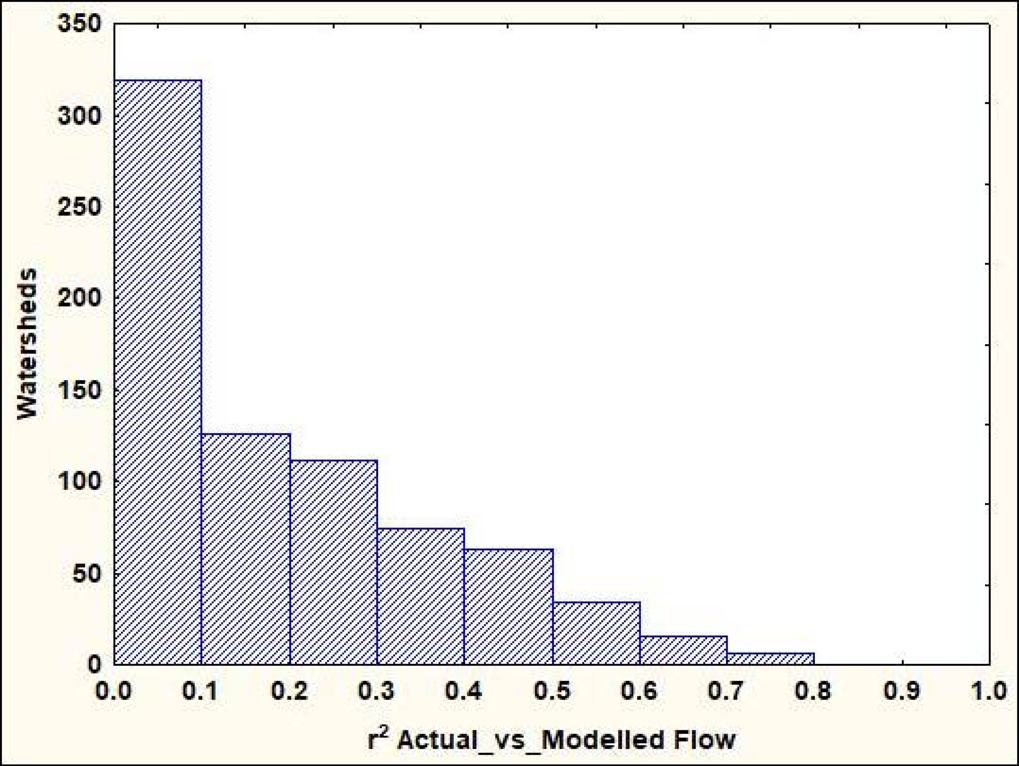
3.1. Analysis of the Fit of the InVEST SWYM
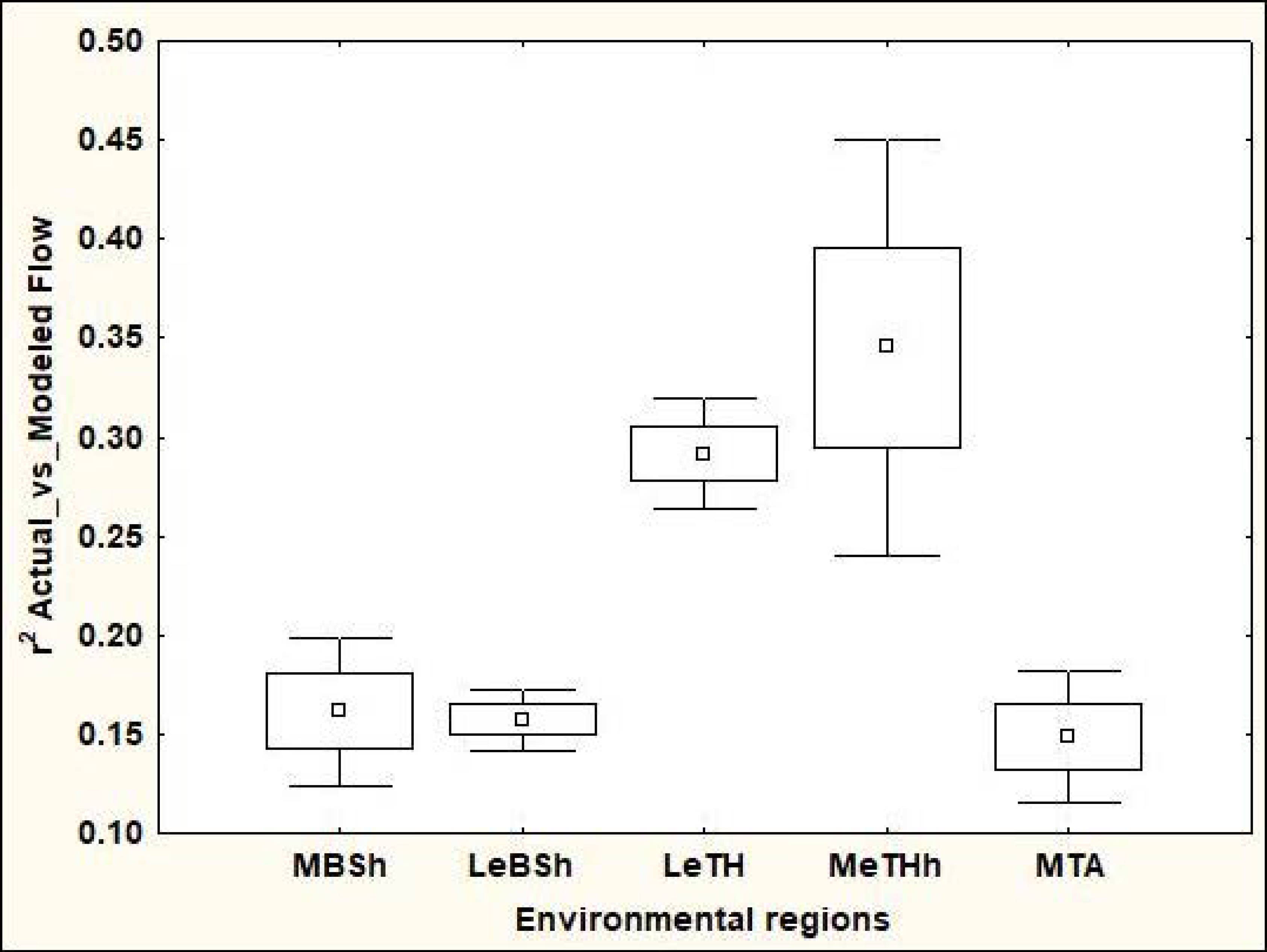
3.2. Analysis of the Fit of InVEST SWYM by Region
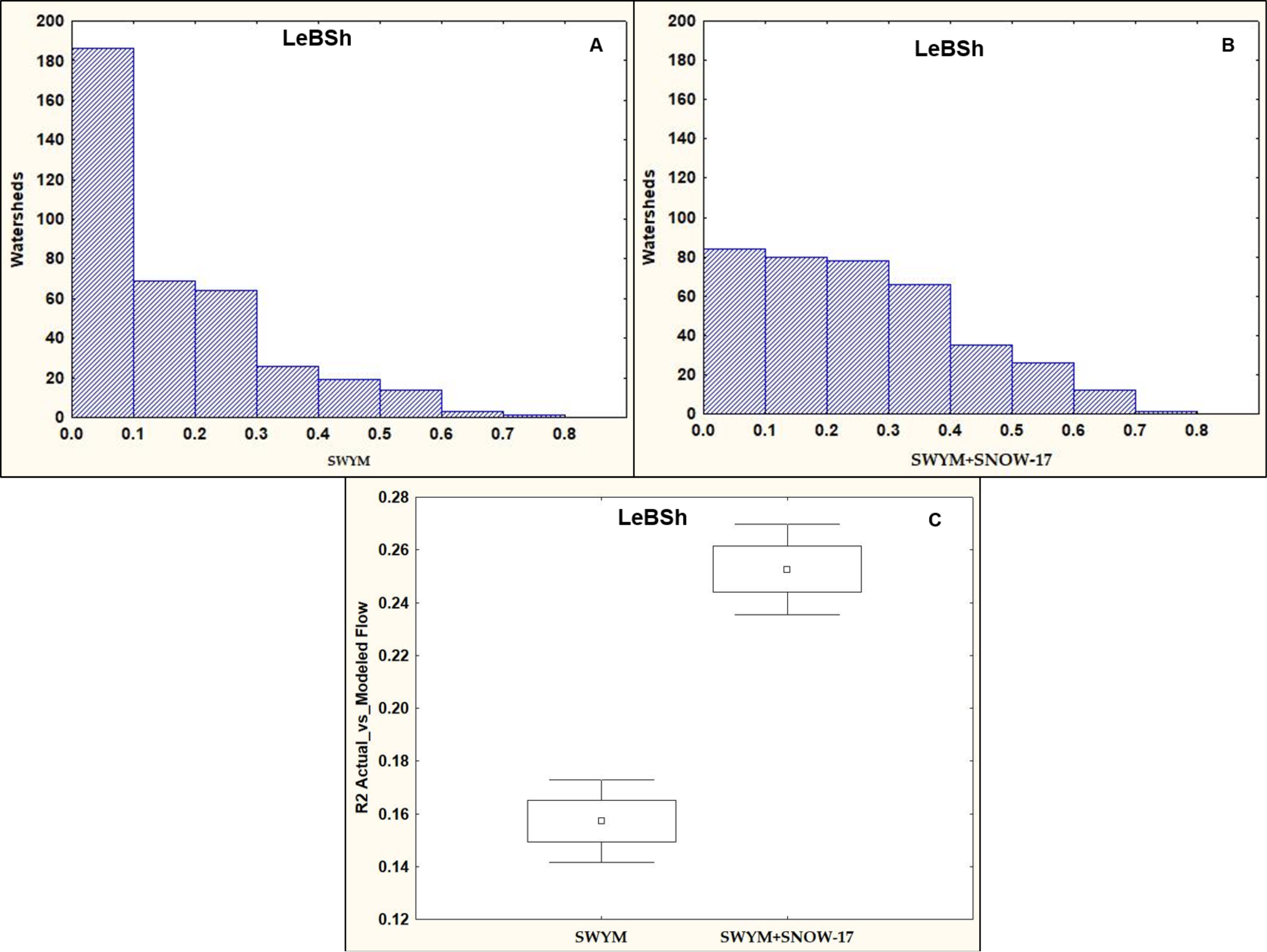
3.3. Analyzing Environmental Features to Improve InVEST SWYM Results
4. Discussion
5. Conclusions
Author Contributions
Funding
Acknowledgments
Conflicts of Interest
Appendix A

Appendix B
| Watershed | Days.below.Zero.Mean | min_elev (m) | max_elev (m) | mean_elev (m) | vapr (kPa) | prec (mm) | srad (kJ) | tmax (°C) | tmin (°C) |
|---|---|---|---|---|---|---|---|---|---|
| 1 | 111.8 | 832.0 | 2392.0 | 1434.5 | 0.6 | 1375.1 | 13,114.6 | 16.8 | −9.5 |
| 2 | 83.4 | 263.0 | 2392.0 | 1023.6 | 0.6 | 952.1 | 13,189.4 | 20.5 | −9.8 |
| 3 | 129.6 | 142.0 | 2654.0 | 1386.2 | 0.6 | 1241.3 | 12,173.8 | 16.5 | −10.0 |
| 4 | 96.7 | 395.0 | 2365.0 | 1026.9 | 0.6 | 1044.3 | 13,062.2 | 19.9 | −10.2 |
| 5 | 111.7 | 314.0 | 2764.0 | 1279.2 | 0.6 | 1380.2 | 12,716.2 | 17.9 | −10.3 |
| 6 | 127.6 | 778.0 | 2734.0 | 1736.9 | 0.5 | 587.2 | 14,364.8 | 17.7 | −10.4 |
| 7 | 78.7 | 589.0 | 3116.0 | 1414.8 | 0.6 | 753.3 | 14,591.0 | 20.4 | −10.4 |
| 8 | 92.1 | 588.0 | 2237.0 | 1106.1 | 0.7 | 824.0 | 13,440.7 | 20.4 | −10.5 |
| 9 | 92.1 | 618.0 | 2237.0 | 1131.5 | 0.7 | 837.1 | 13,445.0 | 20.3 | −10.5 |
| 10 | 97.9 | 651.0 | 2037.0 | 1163.9 | 0.6 | 907.7 | 13,340.9 | 20.0 | −10.5 |
| 11 | 97.9 | 641.0 | 2037.0 | 1176.5 | 0.6 | 915.2 | 13,350.6 | 19.9 | −10.6 |
| 12 | 127.5 | 239.0 | 2687.0 | 1336.9 | 0.5 | 1050.8 | 12,741.9 | 17.5 | −10.7 |
| 13 | 126.4 | 468.0 | 2608.0 | 1826.4 | 0.5 | 710.3 | 12,686.3 | 15.1 | −11.0 |
| 14 | 115.9 | 657.0 | 2237.0 | 1374.3 | 0.6 | 841.9 | 13,492.6 | 19.3 | −11.3 |
| 15 | 123.5 | 636.0 | 2558.0 | 1562.8 | 0.5 | 793.0 | 12,447.8 | 16.3 | −11.3 |
| 16 | 106.1 | 639.0 | 2202.0 | 1345.0 | 0.6 | 654.1 | 12,259.7 | 17.3 | −11.5 |
| 17 | 110.3 | 295.0 | 2608.0 | 1446.3 | 0.5 | 644.8 | 12,515.7 | 17.0 | −11.5 |
| 18 | 130.9 | 529.0 | 2666.0 | 1590.8 | 0.5 | 803.4 | 12,735.1 | 16.6 | −11.5 |
| 19 | 103.6 | 277.0 | 2666.0 | 1424.0 | 0.5 | 726.2 | 12,871.8 | 17.9 | −11.5 |
| 20 | 119.8 | 531.0 | 2558.0 | 1412.4 | 0.5 | 680.7 | 12,390.4 | 16.9 | −11.6 |
| 21 | 81.1 | 592.0 | 2326.0 | 1443.7 | 0.6 | 965.1 | 12,906.3 | 17.5 | −11.9 |
| 22 | 87.7 | 440.0 | 2618.0 | 1584.1 | 0.5 | 524.1 | 13,801.6 | 19.0 | −11.9 |
| 23 | 91.4 | 250.0 | 2284.0 | 1089.1 | 0.6 | 582.8 | 12,602.8 | 18.9 | −12.0 |
| 24 | 100.4 | 287.0 | 2183.0 | 1085.2 | 0.6 | 596.3 | 12,566.3 | 18.8 | −12.1 |
| 25 | 109.1 | 297.0 | 2139.0 | 1077.7 | 0.6 | 606.8 | 12,544.6 | 18.8 | −12.1 |
| 26 | 80.3 | 513.0 | 2325.0 | 1369.4 | 0.6 | 817.9 | 12,808.2 | 17.6 | −12.1 |
| 27 | 71.5 | 312.0 | 2660.0 | 1477.0 | 0.5 | 1111.6 | 11,553.6 | 15.6 | −12.2 |
| 28 | 69.5 | 460.0 | 2707.0 | 1670.1 | 0.5 | 532.8 | 14,004.2 | 19.0 | −12.2 |
| 29 | 91.6 | 333.0 | 2236.0 | 1258.6 | 0.6 | 520.8 | 12,228.1 | 18.0 | −12.3 |
| 30 | 98.3 | 398.0 | 2362.0 | 1290.9 | 0.6 | 700.4 | 12,858.5 | 18.4 | −12.6 |
| 31 | 98.3 | 398.0 | 2362.0 | 1291.0 | 0.6 | 700.4 | 12,858.5 | 18.4 | −12.6 |
| 32 | 105.6 | 633.0 | 2362.0 | 1437.7 | 0.6 | 877.3 | 12,681.9 | 17.0 | −12.8 |
| 33 | 93.0 | 352.0 | 2139.0 | 1377.7 | 0.5 | 810.6 | 12,621.0 | 17.0 | −12.8 |
| 34 | 93.3 | 565.0 | 2362.0 | 1337.1 | 0.6 | 719.8 | 12,794.3 | 17.9 | −12.9 |
| 35 | 109.3 | 648.0 | 2773.0 | 1730.2 | 0.5 | 1165.5 | 12,603.3 | 15.3 | −13.1 |
| 36 | 100.7 | 365.0 | 2776.0 | 1363.5 | 0.5 | 1375.0 | 12,153.5 | 15.7 | −13.4 |
| 37 | 106.7 | 1254.0 | 2961.0 | 1738.3 | 0.5 | 619.2 | 13,308.6 | 18.1 | −13.6 |
| 38 | 101.0 | 337.0 | 2801.0 | 1251.2 | 0.5 | 1035.8 | 12,051.9 | 16.8 | −13.6 |
| 39 | 95.1 | 1064.0 | 3037.0 | 1512.3 | 0.5 | 686.4 | 13,297.1 | 19.1 | −13.7 |
| 40 | 117.3 | 800.0 | 2367.0 | 1461.6 | 0.6 | 759.8 | 13,020.2 | 17.7 | −13.7 |
| 41 | 132.4 | 530.0 | 2832.0 | 1643.2 | 0.5 | 1334.2 | 12,433.4 | 15.6 | −13.8 |
| 42 | 142.6 | 756.0 | 3096.0 | 1628.8 | 0.5 | 599.6 | 11,224.1 | 15.6 | −14.1 |
| 43 | 113.4 | 1190.0 | 2622.0 | 1705.4 | 0.5 | 722.2 | 13,105.8 | 17.7 | −14.2 |
| 44 | 165.4 | 1132.0 | 2649.0 | 1528.8 | 0.4 | 620.4 | 11,826.0 | 16.0 | −14.2 |
| 45 | 122.6 | 657.0 | 2859.0 | 1286.1 | 0.5 | 916.8 | 11,560.2 | 16.3 | −14.2 |
| 46 | 132.8 | 710.0 | 2434.0 | 1334.9 | 0.5 | 1107.3 | 9901.3 | 13.6 | −14.3 |
| 47 | 105.0 | 1090.0 | 2771.0 | 1860.1 | 0.4 | 602.4 | 13,406.9 | 17.6 | −14.3 |
| 48 | 110.1 | 1036.0 | 2915.0 | 1636.5 | 0.5 | 660.9 | 13,099.4 | 17.9 | −14.4 |
| 49 | 130.1 | 834.0 | 3115.0 | 1988.0 | 0.4 | 1068.8 | 12,577.0 | 14.5 | −14.5 |
| 50 | 95.1 | 1233.0 | 3092.0 | 1822.3 | 0.5 | 828.9 | 13,070.7 | 16.9 | −14.5 |
| 51 | 139.9 | 505.0 | 3183.0 | 1729.6 | 0.5 | 1289.7 | 12,419.5 | 15.1 | −14.6 |
| 52 | 160.5 | 1247.0 | 2770.0 | 1812.6 | 0.3 | 688.7 | 11,822.7 | 14.6 | −14.8 |
| 53 | 104.4 | 956.0 | 2975.0 | 1711.1 | 0.5 | 665.0 | 13,184.5 | 18.0 | −14.9 |
| 54 | 156.3 | 1410.0 | 3050.0 | 1983.0 | 0.4 | 691.2 | 12,851.3 | 15.3 | −15.1 |
| 55 | 153.7 | 936.0 | 3252.0 | 1831.5 | 0.3 | 811.8 | 11,574.9 | 14.1 | −15.1 |
| 56 | 156.3 | 1297.0 | 3085.0 | 1942.5 | 0.4 | 654.3 | 12,823.4 | 16.5 | −15.2 |
| 57 | 135.2 | 1030.0 | 3050.0 | 1653.7 | 0.5 | 615.3 | 12,968.0 | 18.0 | −15.3 |
| 58 | 138.9 | 571.0 | 2513.0 | 1215.8 | 0.5 | 719.7 | 11,193.0 | 16.8 | −15.4 |
| 59 | 154.6 | 1035.0 | 2950.0 | 1891.6 | 0.3 | 882.2 | 11,730.4 | 13.3 | −15.4 |
| 60 | 141.3 | 748.0 | 2513.0 | 1319.9 | 0.4 | 804.0 | 11,145.3 | 15.9 | −15.5 |
| 61 | 113.1 | 1054.0 | 3085.0 | 1672.8 | 0.5 | 599.1 | 12,855.9 | 17.7 | −15.6 |
| 62 | 158.9 | 971.0 | 3245.0 | 1901.9 | 0.3 | 908.7 | 11,706.9 | 13.7 | −15.6 |
| 63 | 118.6 | 1212.0 | 2583.0 | 1742.4 | 0.5 | 780.8 | 12,976.9 | 17.0 | −15.7 |
| 64 | 135.2 | 961.0 | 3085.0 | 1536.0 | 0.5 | 585.2 | 12,977.4 | 18.7 | −15.7 |
| 65 | 151.9 | 952.0 | 3627.0 | 1905.3 | 0.3 | 770.0 | 11,886.0 | 14.5 | −15.8 |
| 66 | 154.8 | 2.0 | 2435.0 | 1217.2 | 0.5 | 1263.1 | 9263.4 | 13.7 | −15.8 |
| 67 | 142.4 | 861.0 | 2770.0 | 1405.4 | 0.4 | 620.6 | 11,904.4 | 17.2 | −15.8 |
| 68 | 141.8 | 1218.0 | 2506.0 | 1595.2 | 0.4 | 599.9 | 12,058.2 | 16.2 | −15.8 |
| 69 | 157.6 | 739.0 | 3378.0 | 1760.1 | 0.5 | 946.7 | 12,471.2 | 15.6 | −15.8 |
| 70 | 161.8 | 1296.0 | 3088.0 | 2034.9 | 0.4 | 699.4 | 12,523.6 | 15.2 | −15.8 |
| 71 | 144.0 | 573.0 | 2118.0 | 1200.8 | 0.5 | 792.6 | 10,945.2 | 16.2 | −15.9 |
| 72 | 139.6 | 997.0 | 3177.0 | 1849.2 | 0.4 | 725.2 | 12,837.8 | 15.9 | −15.9 |
| 73 | 158.8 | 1007.0 | 3627.0 | 2010.9 | 0.3 | 853.3 | 11,895.9 | 14.2 | −16.1 |
| 74 | 143.8 | 1368.0 | 3218.0 | 2082.3 | 0.4 | 708.7 | 12,520.9 | 14.8 | −16.1 |
| 75 | 164.5 | 1054.0 | 3094.0 | 1804.1 | 0.4 | 684.1 | 12,451.2 | 16.2 | −16.2 |
| 76 | 150.3 | 1056.0 | 3459.0 | 1872.4 | 0.4 | 686.5 | 12,597.4 | 16.2 | −16.2 |
| 77 | 150.3 | 1027.0 | 3459.0 | 1864.3 | 0.4 | 684.7 | 12,601.1 | 16.3 | −16.3 |
| 78 | 162.3 | 1224.0 | 3459.0 | 2066.6 | 0.4 | 754.2 | 12,485.0 | 14.7 | −16.3 |
| 79 | 174.2 | 1216.0 | 3430.0 | 2136.1 | 0.3 | 887.8 | 12,208.2 | 14.1 | −16.4 |
| 80 | 165.4 | 1176.0 | 3006.0 | 1770.0 | 0.5 | 762.2 | 12,471.5 | 15.9 | −16.6 |
| 81 | 134.7 | 925.0 | 2714.0 | 1404.2 | 0.5 | 595.3 | 12,107.3 | 17.9 | −16.6 |
| 82 | 152.3 | 984.0 | 3277.0 | 1740.1 | 0.4 | 675.0 | 12,512.7 | 16.8 | −16.6 |
| 83 | 168.6 | 1375.0 | 3459.0 | 2127.9 | 0.4 | 826.9 | 12,377.3 | 14.4 | −16.7 |
| 84 | 146.6 | 841.0 | 3251.0 | 1671.3 | 0.4 | 675.8 | 12,227.6 | 16.7 | −16.8 |
| 85 | 140.7 | 766.0 | 3378.0 | 1911.7 | 0.4 | 954.4 | 12,298.4 | 15.2 | −16.8 |
| 86 | 140.4 | 687.0 | 2461.0 | 1131.4 | 0.5 | 843.2 | 10,930.8 | 16.5 | −17.0 |
| 87 | 182.1 | 1341.0 | 3430.0 | 2164.2 | 0.3 | 973.4 | 12,139.1 | 14.0 | −17.0 |
| 88 | 156.7 | 704.0 | 2303.0 | 1330.6 | 0.4 | 658.9 | 10,566.7 | 15.2 | −17.3 |
| 89 | 183.7 | 1536.0 | 3123.0 | 2183.6 | 0.3 | 927.7 | 12,298.2 | 14.4 | −17.8 |
| 90 | 158.9 | 475.0 | 2455.0 | 1138.1 | 0.4 | 607.4 | 10,691.8 | 16.5 | −17.9 |
| 91 | 153.6 | 689.0 | 2042.0 | 1135.1 | 0.5 | 594.7 | 10,508.4 | 16.1 | −18.3 |
| 92 | 170.3 | 786.0 | 2780.0 | 1431.8 | 0.4 | 646.8 | 10,382.5 | 15.0 | −18.5 |
| 93 | 160.3 | 736.0 | 2307.0 | 1289.7 | 0.4 | 608.2 | 10,166.0 | 15.1 | −19.1 |
| 94 | 168.9 | 806.0 | 2356.0 | 1382.5 | 0.4 | 596.8 | 10,158.9 | 14.8 | −19.4 |
| 95 | 171.9 | 1680.0 | 2093.0 | 1881.8 | 0.4 | 526.9 | 9147.8 | 13.6 | −19.4 |
| 96 | 178.1 | 795.0 | 2141.0 | 1340.8 | 0.4 | 574.9 | 8816.6 | 14.3 | −19.4 |
| 97 | 168.1 | 725.0 | 2332.0 | 1406.2 | 0.4 | 601.0 | 10,089.3 | 14.5 | −19.5 |
| 98 | 188.5 | 678.0 | 2324.0 | 1491.3 | 0.4 | 608.7 | 9919.3 | 14.2 | −19.9 |
| 99 | 179.3 | 712.0 | 2533.0 | 1473.1 | 0.4 | 666.5 | 10,157.7 | 14.5 | −20.1 |
| 100 | 150.7 | 645.0 | 2123.0 | 1224.6 | 0.4 | 630.4 | 9175.7 | 13.7 | −20.2 |
| 101 | 161.1 | 620.0 | 2360.0 | 1146.6 | 0.4 | 527.9 | 9271.7 | 15.1 | −20.6 |
| 102 | 179.4 | 756.0 | 2401.0 | 1522.0 | 0.4 | 469.1 | 9005.2 | 14.6 | −20.6 |
| 103 | 206.7 | 759.0 | 2771.0 | 1541.2 | 0.3 | 650.1 | 9987.1 | 14.1 | −20.6 |
| 104 | 199.3 | 785.0 | 2069.0 | 1381.1 | 0.4 | 620.8 | 9242.8 | 14.6 | −20.9 |
| 105 | 217.3 | 520.0 | 2298.0 | 1356.3 | 0.4 | 571.4 | 9713.3 | 15.3 | −21.0 |
| 106 | 222.3 | 715.0 | 2710.0 | 1573.6 | 0.3 | 616.7 | 9693.9 | 14.2 | −21.0 |
| 107 | 192.4 | 869.0 | 2201.0 | 1328.9 | 0.4 | 546.3 | 9332.2 | 16.0 | −23.1 |
| 108 | 184.2 | 908.0 | 1982.0 | 1288.3 | 0.4 | 534.0 | 9404.4 | 16.6 | −23.5 |
| 109 | 33.7 | 294.0 | 611.0 | 417.1 | 1.1 | 767.6 | 16,022.2 | 34.0 | −6.9 |
| 110 | 40.3 | 336.0 | 505.0 | 418.4 | 1.1 | 855.4 | 15,635.2 | 32.8 | −7.4 |
| 111 | 39.7 | 448.0 | 670.0 | 552.6 | 1.0 | 671.9 | 16,219.2 | 33.6 | −7.8 |
| 112 | 58.6 | −23.0 | 204.0 | 70.4 | 1.0 | 1237.8 | 13,436.4 | 26.6 | −7.8 |
| 113 | 44.4 | 273.0 | 506.0 | 392.4 | 1.1 | 896.5 | 15,325.2 | 32.2 | −8.3 |
| 114 | 54.3 | −26.0 | 631.0 | 170.2 | 1.0 | 1151.4 | 13,444.4 | 28.0 | −8.6 |
| 115 | 64.1 | 42.0 | 631.0 | 206.4 | 1.0 | 1152.5 | 13,353.4 | 27.6 | −9.1 |
| 116 | 46.3 | 620.0 | 903.0 | 765.8 | 1.0 | 542.2 | 16,615.3 | 33.6 | −9.3 |
| 117 | 62.9 | 92.0 | 949.0 | 378.1 | 1.0 | 1009.9 | 13,102.7 | 26.7 | −9.5 |
| 118 | 53.3 | 364.0 | 1063.0 | 628.1 | 1.0 | 615.7 | 15,958.4 | 33.1 | −9.9 |
| 119 | 70.2 | 185.0 | 949.0 | 427.1 | 1.0 | 1002.4 | 12,974.1 | 26.2 | −9.9 |
| 120 | 106.4 | 24.0 | 207.0 | 109.4 | 0.8 | 1477.3 | 12,518.3 | 22.0 | −10.0 |
| 121 | 94.6 | −3.0 | 308.0 | 80.8 | 0.8 | 1548.8 | 11,086.5 | 18.8 | −10.1 |
| 122 | 54.9 | 794.0 | 1465.0 | 1105.0 | 0.8 | 441.0 | 16,670.5 | 32.5 | −10.2 |
| 123 | 65.3 | 47.0 | 396.0 | 191.6 | 0.9 | 1247.0 | 13,199.6 | 26.2 | −10.5 |
| 124 | 74.9 | 175.0 | 425.0 | 292.8 | 1.0 | 1037.7 | 12,833.2 | 25.6 | −10.6 |
| 125 | 61.9 | 49.0 | 525.0 | 189.7 | 1.0 | 1212.0 | 13,223.2 | 27.4 | −10.6 |
| 126 | 71.3 | 186.0 | 343.0 | 243.7 | 1.0 | 888.6 | 13,133.3 | 27.7 | −10.8 |
| 127 | 93.0 | 168.0 | 373.0 | 239.8 | 0.9 | 800.4 | 12,738.6 | 26.2 | −11.2 |
| 128 | 65.8 | 352.0 | 681.0 | 512.8 | 1.0 | 723.4 | 15,173.8 | 31.3 | −11.2 |
| 129 | 75.8 | 186.0 | 311.0 | 250.2 | 1.0 | 962.6 | 13,172.3 | 27.4 | −11.4 |
| 130 | 72.5 | 255.0 | 413.0 | 336.7 | 1.1 | 897.2 | 14,381.4 | 30.0 | −11.5 |
| 131 | 78.4 | 172.0 | 798.0 | 526.4 | 0.9 | 1065.3 | 12,773.0 | 24.9 | −11.5 |
| 132 | 77.0 | 315.0 | 576.0 | 420.8 | 0.9 | 1142.1 | 12,753.9 | 24.8 | −11.5 |
| 133 | 81.0 | 304.0 | 648.0 | 475.8 | 0.9 | 1114.5 | 12,795.6 | 25.3 | −11.6 |
| 134 | 64.3 | 788.0 | 1368.0 | 1068.9 | 0.8 | 461.0 | 15,814.3 | 31.3 | −11.6 |
| 135 | 76.0 | 145.0 | 295.0 | 223.4 | 1.0 | 978.4 | 13,166.1 | 27.5 | −11.7 |
| 136 | 94.5 | 24.0 | 283.0 | 171.1 | 0.8 | 1390.5 | 12,385.3 | 22.5 | −11.7 |
| 137 | 89.5 | 173.0 | 299.0 | 223.9 | 0.9 | 970.1 | 12,772.1 | 24.7 | −11.7 |
| 138 | 85.1 | 231.0 | 366.0 | 284.6 | 0.9 | 810.5 | 12,781.8 | 26.1 | −11.7 |
| 139 | 71.9 | 194.0 | 422.0 | 316.0 | 1.1 | 913.1 | 14,201.4 | 29.6 | −11.7 |
| 140 | 71.1 | 275.0 | 444.0 | 353.5 | 1.0 | 813.7 | 14,630.9 | 30.7 | −11.7 |
| 141 | 72.9 | 142.0 | 295.0 | 219.7 | 1.0 | 979.0 | 13,196.0 | 27.6 | −11.7 |
| 142 | 91.5 | 195.0 | 299.0 | 234.5 | 0.9 | 974.9 | 12,764.4 | 24.6 | −11.7 |
| 143 | 68.3 | 142.0 | 277.0 | 205.2 | 1.1 | 957.0 | 13,434.3 | 28.3 | −11.8 |
| 144 | 69.6 | 501.0 | 681.0 | 601.9 | 1.0 | 676.1 | 15,244.7 | 31.1 | −11.8 |
| 145 | 82.0 | 177.0 | 368.0 | 249.2 | 1.0 | 862.5 | 12,867.2 | 26.7 | −11.8 |
| 146 | 80.6 | 213.0 | 378.0 | 277.3 | 1.0 | 912.0 | 12,870.4 | 26.4 | −11.8 |
| 147 | 86.1 | 2.0 | 780.0 | 296.8 | 0.9 | 1189.8 | 13,020.4 | 26.0 | −11.9 |
| 148 | 71.4 | 329.0 | 514.0 | 399.8 | 1.0 | 759.2 | 14,680.7 | 30.6 | −12.0 |
| 149 | 90.1 | 154.0 | 411.0 | 289.1 | 0.9 | 1003.9 | 12,772.5 | 24.3 | −12.1 |
| 150 | 83.0 | 219.0 | 383.0 | 297.5 | 1.0 | 870.2 | 12,788.8 | 26.3 | −12.1 |
| 151 | 78.3 | 31.0 | 566.0 | 231.8 | 0.9 | 1145.5 | 13,067.3 | 25.8 | −12.2 |
| 152 | 94.8 | 200.0 | 326.0 | 262.0 | 0.9 | 1012.6 | 12,740.9 | 24.2 | −12.2 |
| 153 | 71.6 | 117.0 | 287.0 | 212.5 | 1.0 | 945.5 | 13,818.4 | 28.7 | −12.2 |
| 154 | 86.5 | 237.0 | 352.0 | 281.5 | 0.9 | 802.3 | 12,746.7 | 26.2 | −12.2 |
| 155 | 85.1 | 211.0 | 366.0 | 264.9 | 0.9 | 770.6 | 12,734.4 | 25.9 | −12.2 |
| 156 | 90.2 | −12.0 | 351.0 | 106.7 | 0.9 | 1073.4 | 13,017.0 | 26.2 | −12.3 |
| 157 | 113.8 | −21.0 | 307.0 | 138.0 | 0.8 | 1443.9 | 12,170.8 | 21.7 | −12.3 |
| 158 | 86.1 | 134.0 | 366.0 | 254.3 | 0.9 | 771.1 | 12,727.1 | 25.9 | −12.3 |
| 159 | 83.8 | 231.0 | 791.0 | 492.4 | 0.9 | 897.8 | 12,595.8 | 24.3 | −12.4 |
| 160 | 76.5 | 130.0 | 287.0 | 218.7 | 1.0 | 945.8 | 13,788.5 | 28.6 | −12.4 |
| 161 | 88.8 | 93.0 | 1236.0 | 490.3 | 0.9 | 1137.2 | 12,845.1 | 24.3 | −12.4 |
| 162 | 78.9 | 559.0 | 1007.0 | 777.3 | 0.9 | 585.2 | 15,076.3 | 30.3 | −12.6 |
| 163 | 100.1 | 217.0 | 411.0 | 318.2 | 0.9 | 1025.9 | 12,752.9 | 23.9 | −12.6 |
| 164 | 102.9 | 221.0 | 359.0 | 293.4 | 0.9 | 1069.2 | 12,706.8 | 23.6 | −12.6 |
| 165 | 96.9 | 207.0 | 303.0 | 234.1 | 0.9 | 758.0 | 12,675.5 | 24.8 | −12.6 |
| 166 | 100.3 | 267.0 | 652.0 | 444.2 | 0.9 | 1056.2 | 12,519.7 | 24.0 | −12.6 |
| 167 | 84.6 | 63.0 | 780.0 | 343.8 | 0.9 | 1171.7 | 12,944.6 | 25.5 | −12.6 |
| 168 | 98.1 | 71.0 | 640.0 | 252.1 | 0.9 | 1134.0 | 12,482.5 | 24.5 | −12.7 |
| 169 | 82.3 | 925.0 | 1504.0 | 1155.7 | 0.7 | 409.3 | 15,110.3 | 29.7 | −12.8 |
| 170 | 100.2 | 281.0 | 1004.0 | 548.4 | 0.9 | 1085.5 | 12,653.4 | 23.8 | −12.9 |
| 171 | 93.9 | 427.0 | 795.0 | 604.8 | 0.9 | 1064.8 | 12,588.4 | 23.6 | −12.9 |
| 172 | 91.3 | 230.0 | 706.0 | 491.5 | 0.9 | 1067.0 | 12,547.3 | 23.7 | −13.0 |
| 173 | 123.7 | 32.0 | 351.0 | 192.7 | 0.7 | 1428.9 | 11,021.9 | 19.6 | −13.0 |
| 174 | 100.1 | 292.0 | 1166.0 | 621.0 | 0.8 | 1150.6 | 12,697.6 | 23.4 | −13.0 |
| 175 | 79.3 | 780.0 | 1304.0 | 1058.8 | 0.8 | 494.7 | 15,036.9 | 29.8 | −13.0 |
| 176 | 94.5 | 404.0 | 795.0 | 583.9 | 0.9 | 1062.1 | 12,568.8 | 23.6 | −13.0 |
| 177 | 97.4 | 243.0 | 817.0 | 470.8 | 0.9 | 1068.7 | 12,603.5 | 24.1 | −13.0 |
| 178 | 79.5 | 688.0 | 1227.0 | 905.6 | 0.8 | 536.0 | 14,866.2 | 29.8 | −13.2 |
| 179 | 107.6 | 144.0 | 351.0 | 229.5 | 0.9 | 1033.3 | 12,646.2 | 22.4 | −13.2 |
| 180 | 76.6 | 275.0 | 470.0 | 371.2 | 1.0 | 837.8 | 14,176.4 | 29.3 | −13.2 |
| 181 | 130.2 | 5.0 | 347.0 | 199.1 | 0.7 | 1601.6 | 11,043.4 | 19.6 | −13.3 |
| 182 | 108.1 | 245.0 | 436.0 | 354.4 | 0.9 | 970.6 | 12,771.5 | 23.5 | −13.3 |
| 183 | 89.2 | 327.0 | 785.0 | 564.2 | 0.9 | 985.1 | 12,547.1 | 23.6 | −13.3 |
| 184 | 79.9 | 150.0 | 304.0 | 213.2 | 1.0 | 940.4 | 13,625.8 | 28.1 | −13.4 |
| 185 | 108.1 | 331.0 | 436.0 | 379.6 | 0.9 | 988.0 | 12,754.3 | 23.3 | −13.5 |
| 186 | 100.7 | 185.0 | 536.0 | 380.6 | 0.9 | 957.4 | 12,763.7 | 23.1 | −13.6 |
| 187 | 97.8 | 212.0 | 381.0 | 294.2 | 0.9 | 808.7 | 12,628.7 | 25.1 | −13.9 |
| 188 | 98.1 | 170.0 | 476.0 | 255.4 | 0.9 | 781.1 | 12,609.4 | 25.1 | −14.0 |
| 189 | 86.1 | 174.0 | 364.0 | 263.5 | 1.0 | 918.0 | 13,284.9 | 27.1 | −14.1 |
| 190 | 135.5 | 42.0 | 530.0 | 359.7 | 0.8 | 1572.3 | 11,655.9 | 19.8 | −14.1 |
| 191 | 98.5 | 189.0 | 522.0 | 315.1 | 0.9 | 862.6 | 12,746.0 | 23.1 | −14.1 |
| 192 | 84.9 | 1240.0 | 1820.0 | 1431.6 | 0.6 | 353.4 | 14,867.8 | 27.9 | −14.3 |
| 193 | 86.1 | 199.0 | 378.0 | 291.9 | 1.0 | 865.5 | 13,755.2 | 28.5 | −14.3 |
| 194 | 95.7 | 135.0 | 395.0 | 279.2 | 0.9 | 813.6 | 13,016.1 | 25.3 | −14.3 |
| 195 | 88.9 | 917.0 | 1424.0 | 1111.6 | 0.7 | 376.3 | 14,419.2 | 28.1 | −14.3 |
| 196 | 98.7 | 178.0 | 521.0 | 339.9 | 0.9 | 814.5 | 12,566.8 | 24.6 | −14.3 |
| 197 | 88.1 | 1036.0 | 1499.0 | 1244.4 | 0.6 | 366.2 | 14,665.2 | 28.2 | −14.3 |
| 198 | 113.5 | 15.0 | 1561.0 | 308.8 | 0.8 | 1118.0 | 12,800.0 | 24.7 | −14.4 |
| 199 | 85.7 | 309.0 | 464.0 | 396.1 | 1.0 | 792.6 | 13,988.3 | 28.6 | −14.4 |
| 200 | 90.3 | 438.0 | 969.0 | 669.6 | 0.8 | 434.9 | 14,373.6 | 30.3 | −14.4 |
| 201 | 108.2 | 858.0 | 1398.0 | 1115.0 | 0.6 | 413.8 | 13,491.2 | 22.8 | −14.5 |
| 202 | 103.7 | 12.0 | 329.0 | 154.2 | 0.8 | 1290.6 | 12,435.1 | 22.3 | −14.7 |
| 203 | 115.7 | 161.0 | 414.0 | 257.9 | 0.9 | 966.1 | 12,696.1 | 23.1 | −14.7 |
| 204 | 139.7 | 831.0 | 1994.0 | 1171.1 | 0.5 | 653.2 | 11,374.0 | 17.4 | −14.8 |
| 205 | 86.4 | 199.0 | 459.0 | 353.7 | 1.0 | 818.1 | 13,853.2 | 28.5 | −14.8 |
| 206 | 136.1 | 811.0 | 1634.0 | 1176.9 | 0.4 | 594.3 | 11,659.2 | 17.8 | −14.8 |
| 207 | 111.3 | 67.0 | 1252.0 | 404.5 | 0.8 | 1123.0 | 12,555.6 | 23.7 | −14.9 |
| 208 | 89.9 | 198.0 | 378.0 | 290.9 | 1.0 | 882.0 | 13,438.2 | 27.2 | −14.9 |
| 209 | 106.5 | 175.0 | 439.0 | 273.5 | 0.8 | 717.6 | 12,460.3 | 23.9 | −15.1 |
| 210 | 125.3 | 57.0 | 1561.0 | 372.4 | 0.8 | 1148.9 | 12,678.9 | 23.9 | −15.1 |
| 211 | 92.9 | 185.0 | 393.0 | 273.8 | 0.9 | 830.4 | 13,138.1 | 26.3 | −15.2 |
| 212 | 98.6 | 686.0 | 1221.0 | 873.8 | 0.7 | 432.2 | 14,259.9 | 28.5 | −15.2 |
| 213 | 136.1 | 706.0 | 1292.0 | 900.4 | 0.5 | 562.5 | 11,703.3 | 19.2 | −15.3 |
| 214 | 89.5 | 283.0 | 459.0 | 368.7 | 1.0 | 799.8 | 13,798.5 | 28.3 | −15.4 |
| 215 | 137.4 | −1.0 | 758.0 | 320.0 | 0.7 | 1219.2 | 10,857.6 | 18.3 | −15.6 |
| 216 | 115.0 | 82.0 | 1084.0 | 469.2 | 0.8 | 1240.7 | 12,368.2 | 22.9 | −15.7 |
| 217 | 114.5 | 57.0 | 761.0 | 317.9 | 0.8 | 1045.4 | 12,410.9 | 23.8 | −15.7 |
| 218 | 156.8 | 128.0 | 1664.0 | 545.7 | 0.8 | 1309.0 | 12,529.6 | 22.5 | −15.7 |
| 219 | 105.3 | 33.0 | 385.0 | 115.4 | 0.9 | 953.1 | 12,491.4 | 24.4 | −15.7 |
| 220 | 96.9 | 263.0 | 408.0 | 343.5 | 1.0 | 844.8 | 13,563.2 | 27.8 | −15.8 |
| 221 | 112.5 | 979.0 | 1572.0 | 1142.3 | 0.6 | 470.0 | 13,137.9 | 21.7 | −15.8 |
| 222 | 112.1 | 154.0 | 335.0 | 232.0 | 0.8 | 819.3 | 12,285.3 | 22.2 | −15.9 |
| 223 | 96.2 | 299.0 | 507.0 | 409.9 | 0.9 | 730.1 | 13,798.0 | 28.1 | −15.9 |
| 224 | 121.2 | 81.0 | 455.0 | 228.1 | 0.9 | 936.5 | 12,585.6 | 23.6 | −15.9 |
| 225 | 109.0 | 20.0 | 232.0 | 116.7 | 0.8 | 1182.4 | 12,402.6 | 23.2 | −15.9 |
| 226 | 118.1 | 16.0 | 174.0 | 83.8 | 0.8 | 1151.4 | 12,303.1 | 23.1 | −16.0 |
| 227 | 96.9 | 337.0 | 480.0 | 415.5 | 0.9 | 691.3 | 13,835.8 | 28.3 | −16.2 |
| 228 | 128.6 | 289.0 | 1587.0 | 625.1 | 0.8 | 1149.5 | 12,358.6 | 22.1 | −16.2 |
| 229 | 139.5 | 825.0 | 1370.0 | 1140.6 | 0.5 | 611.4 | 11,857.1 | 18.7 | −16.2 |
| 230 | 116.8 | 186.0 | 354.0 | 240.8 | 0.8 | 810.2 | 12,287.3 | 22.2 | −16.2 |
| 231 | 92.7 | 200.0 | 422.0 | 334.9 | 0.9 | 873.1 | 13,289.3 | 26.7 | −16.2 |
| 232 | 113.0 | 81.0 | 1298.0 | 367.4 | 0.8 | 1140.7 | 12,351.0 | 22.9 | −16.3 |
| 233 | 109.7 | 36.0 | 1358.0 | 492.7 | 0.8 | 1039.1 | 12,335.1 | 22.4 | −16.3 |
| 234 | 144.3 | 2.0 | 539.0 | 265.4 | 0.6 | 1184.1 | 10,589.6 | 17.0 | −16.3 |
| 235 | 118.2 | 12.0 | 1896.0 | 422.3 | 0.8 | 1135.1 | 12,470.1 | 22.9 | −16.3 |
| 236 | 113.0 | 902.0 | 1572.0 | 1050.7 | 0.6 | 444.3 | 13,183.2 | 22.1 | −16.4 |
| 237 | 99.3 | 293.0 | 397.0 | 347.8 | 1.0 | 798.8 | 13,570.2 | 27.7 | −16.4 |
| 238 | 136.1 | 599.0 | 2047.0 | 980.8 | 0.5 | 613.0 | 11,008.3 | 17.6 | −16.4 |
| 239 | 107.5 | 769.0 | 1572.0 | 994.2 | 0.6 | 415.7 | 13,256.1 | 22.7 | −16.4 |
| 240 | 142.6 | 124.0 | 1085.0 | 346.1 | 0.8 | 1255.4 | 12,277.7 | 22.5 | −16.5 |
| 241 | 99.1 | 324.0 | 507.0 | 426.7 | 0.9 | 728.9 | 13,683.2 | 27.6 | −16.5 |
| 242 | 107.5 | 808.0 | 1572.0 | 1005.1 | 0.6 | 422.2 | 13,228.7 | 22.5 | −16.5 |
| 243 | 100.9 | 712.0 | 1097.0 | 870.6 | 0.6 | 307.7 | 13,940.6 | 27.8 | −16.5 |
| 244 | 123.9 | 80.0 | 1827.0 | 457.0 | 0.8 | 1118.3 | 12,364.6 | 22.7 | −16.5 |
| 245 | 138.5 | 635.0 | 1592.0 | 885.5 | 0.5 | 699.8 | 11,008.9 | 18.3 | −16.6 |
| 246 | 104.1 | 246.0 | 430.0 | 352.4 | 0.9 | 825.4 | 13,360.8 | 27.2 | −16.6 |
| 247 | 113.7 | 70.0 | 391.0 | 156.0 | 0.8 | 1103.5 | 12,370.8 | 23.6 | −16.7 |
| 248 | 106.8 | 317.0 | 574.0 | 458.2 | 0.9 | 611.2 | 13,854.8 | 28.2 | −16.8 |
| 249 | 99.3 | 240.0 | 436.0 | 354.8 | 0.9 | 843.7 | 13,290.1 | 26.9 | −16.9 |
| 250 | 133.0 | 655.0 | 1610.0 | 1054.4 | 0.5 | 586.5 | 11,914.1 | 19.1 | −16.9 |
| 251 | 130.7 | 151.0 | 1029.0 | 436.9 | 0.8 | 1092.8 | 12,325.7 | 22.7 | −16.9 |
| 252 | 139.8 | 492.0 | 1656.0 | 889.3 | 0.5 | 557.6 | 11,841.4 | 19.7 | −16.9 |
| 253 | 97.9 | 751.0 | 1995.0 | 950.3 | 0.6 | 324.4 | 13,717.7 | 26.0 | −17.0 |
| 254 | 132.5 | 609.0 | 1524.0 | 844.6 | 0.5 | 607.4 | 10,984.0 | 18.4 | −17.1 |
| 255 | 136.9 | 975.0 | 1560.0 | 1148.7 | 0.5 | 598.0 | 12,148.0 | 19.3 | −17.1 |
| 256 | 130.5 | 651.0 | 1201.0 | 847.8 | 0.5 | 576.2 | 11,916.9 | 20.0 | −17.1 |
| 257 | 114.9 | 754.0 | 1010.0 | 841.6 | 0.7 | 406.3 | 13,874.9 | 26.9 | −17.1 |
| 258 | 139.3 | 692.0 | 1026.0 | 823.6 | 0.5 | 480.9 | 11,549.4 | 19.5 | −17.1 |
| 259 | 104.1 | 289.0 | 436.0 | 367.1 | 0.9 | 824.9 | 13,253.5 | 26.7 | −17.2 |
| 260 | 145.9 | 545.0 | 990.0 | 790.2 | 0.5 | 478.5 | 11,463.1 | 19.4 | −17.3 |
| 261 | 114.1 | 576.0 | 1010.0 | 771.4 | 0.7 | 416.9 | 13,850.2 | 27.3 | −17.3 |
| 262 | 134.7 | 819.0 | 2714.0 | 1179.9 | 0.5 | 586.9 | 12,159.2 | 19.1 | −17.4 |
| 263 | 115.9 | 741.0 | 1033.0 | 821.2 | 0.7 | 409.3 | 13,816.0 | 27.0 | −17.5 |
| 264 | 134.3 | 178.0 | 704.0 | 387.8 | 0.8 | 1203.9 | 12,226.3 | 22.2 | −17.5 |
| 265 | 135.8 | 943.0 | 1414.0 | 1083.4 | 0.5 | 594.8 | 12,126.1 | 19.8 | −17.5 |
| 266 | 104.1 | 228.0 | 412.0 | 326.3 | 0.9 | 758.5 | 13,232.1 | 26.9 | −17.6 |
| 267 | 117.7 | 205.0 | 577.0 | 342.6 | 0.8 | 791.1 | 12,593.6 | 24.4 | −17.6 |
| 268 | 138.5 | 174.0 | 489.0 | 332.2 | 0.8 | 943.3 | 12,422.7 | 22.3 | −17.6 |
| 269 | 134.9 | 714.0 | 2714.0 | 1121.4 | 0.5 | 584.6 | 12,151.4 | 19.1 | −17.7 |
| 270 | 126.2 | 197.0 | 480.0 | 323.8 | 0.8 | 793.6 | 12,338.5 | 23.6 | −17.7 |
| 271 | 149.9 | 926.0 | 2007.0 | 1255.7 | 0.5 | 604.3 | 12,407.3 | 19.4 | −17.7 |
| 272 | 126.9 | 258.0 | 1117.0 | 534.9 | 0.8 | 1163.1 | 12,191.4 | 21.6 | −17.7 |
| 273 | 152.9 | 989.0 | 1976.0 | 1263.3 | 0.5 | 603.2 | 12,588.7 | 20.1 | −17.7 |
| 274 | 133.2 | 907.0 | 1865.0 | 1181.0 | 0.5 | 496.8 | 12,807.1 | 20.9 | −17.8 |
| 275 | 125.0 | 266.0 | 1089.0 | 498.9 | 0.7 | 1293.3 | 12,164.3 | 21.4 | −17.8 |
| 276 | 125.2 | 739.0 | 1424.0 | 1047.9 | 0.6 | 383.0 | 13,520.8 | 23.2 | −17.8 |
| 277 | 118.2 | 17.0 | 544.0 | 228.1 | 0.8 | 1130.1 | 12,280.3 | 22.0 | −17.9 |
| 278 | 142.7 | 719.0 | 1214.0 | 857.0 | 0.5 | 554.6 | 10,820.6 | 18.4 | −17.9 |
| 279 | 121.7 | 660.0 | 911.0 | 783.6 | 0.7 | 414.9 | 13,712.5 | 26.7 | −17.9 |
| 280 | 144.5 | 883.0 | 1546.0 | 1109.4 | 0.5 | 614.8 | 12,504.5 | 20.2 | −18.0 |
| 281 | 125.2 | 734.0 | 1335.0 | 905.2 | 0.6 | 393.5 | 13,521.2 | 23.7 | −18.1 |
| 282 | 120.9 | 90.0 | 1262.0 | 441.7 | 0.7 | 1073.2 | 12,327.9 | 21.9 | −18.2 |
| 283 | 137.8 | 875.0 | 1186.0 | 1016.9 | 0.5 | 574.6 | 12,270.3 | 20.1 | −18.2 |
| 284 | 118.9 | 503.0 | 911.0 | 708.7 | 0.7 | 425.1 | 13,655.2 | 26.8 | −18.3 |
| 285 | 113.1 | 181.0 | 536.0 | 333.4 | 0.9 | 835.6 | 12,756.8 | 25.1 | −18.4 |
| 286 | 121.5 | 564.0 | 924.0 | 688.3 | 0.7 | 423.7 | 13,614.9 | 26.8 | −18.4 |
| 287 | 134.9 | 720.0 | 2338.0 | 1037.8 | 0.5 | 588.4 | 12,313.2 | 19.9 | −18.4 |
| 288 | 142.1 | 855.0 | 1133.0 | 976.3 | 0.5 | 590.4 | 12,557.1 | 20.5 | −18.4 |
| 289 | 125.2 | 173.0 | 677.0 | 342.0 | 0.8 | 1264.8 | 12,250.5 | 21.9 | −18.5 |
| 290 | 134.5 | 732.0 | 978.0 | 827.6 | 0.6 | 368.7 | 13,380.9 | 25.8 | −18.5 |
| 291 | 113.8 | 262.0 | 425.0 | 330.9 | 0.9 | 703.9 | 13,055.5 | 26.8 | −18.6 |
| 292 | 132.6 | 306.0 | 539.0 | 400.0 | 0.8 | 1010.2 | 12,458.4 | 21.6 | −18.6 |
| 293 | 121.4 | 525.0 | 997.0 | 672.2 | 0.7 | 425.2 | 13,573.7 | 26.7 | −18.7 |
| 294 | 139.1 | 875.0 | 1065.0 | 972.3 | 0.6 | 585.9 | 12,319.8 | 20.3 | −18.7 |
| 295 | 119.9 | 298.0 | 536.0 | 399.7 | 0.8 | 829.1 | 12,607.8 | 24.3 | −18.9 |
| 296 | 136.3 | 660.0 | 1140.0 | 835.4 | 0.6 | 538.5 | 11,989.7 | 20.1 | −18.9 |
| 297 | 120.0 | 83.0 | 517.0 | 244.9 | 0.8 | 863.3 | 12,529.8 | 22.9 | −19.0 |
| 298 | 147.6 | 575.0 | 1067.0 | 797.1 | 0.6 | 500.3 | 11,865.2 | 20.2 | −19.0 |
| 299 | 149.7 | 718.0 | 1194.0 | 905.6 | 0.6 | 561.6 | 12,094.4 | 19.9 | −19.1 |
| 300 | 136.1 | 748.0 | 993.0 | 889.6 | 0.6 | 362.1 | 13,455.2 | 26.9 | −19.1 |
| 301 | 115.4 | 203.0 | 547.0 | 352.2 | 0.8 | 816.3 | 12,660.2 | 25.2 | −19.1 |
| 302 | 139.9 | 785.0 | 1002.0 | 876.9 | 0.6 | 501.4 | 12,639.6 | 20.8 | −19.1 |
| 303 | 125.6 | 208.0 | 568.0 | 398.3 | 0.8 | 831.2 | 12,255.0 | 23.5 | −19.2 |
| 304 | 135.3 | 838.0 | 1160.0 | 972.3 | 0.6 | 414.2 | 13,520.6 | 23.1 | −19.2 |
| 305 | 131.7 | 313.0 | 598.0 | 473.9 | 0.8 | 804.1 | 12,169.8 | 22.8 | −19.2 |
| 306 | 130.9 | 61.0 | 914.0 | 404.6 | 0.7 | 1176.5 | 12,244.6 | 21.2 | −19.2 |
| 307 | 129.6 | 654.0 | 925.0 | 792.1 | 0.6 | 531.3 | 12,501.4 | 21.1 | −19.3 |
| 308 | 147.6 | 589.0 | 1379.0 | 826.5 | 0.6 | 518.7 | 11,860.0 | 20.2 | −19.4 |
| 309 | 139.9 | 842.0 | 1105.0 | 936.1 | 0.6 | 517.0 | 12,636.5 | 20.6 | −19.4 |
| 310 | 127.3 | 9.0 | 754.0 | 371.1 | 0.7 | 1151.1 | 12,148.3 | 20.8 | −19.4 |
| 311 | 122.3 | 314.0 | 553.0 | 422.6 | 0.8 | 830.2 | 12,410.4 | 23.8 | −19.4 |
| 312 | 120.2 | 256.0 | 385.0 | 321.8 | 0.8 | 562.3 | 13,077.7 | 26.8 | −19.5 |
| 313 | 122.1 | 159.0 | 527.0 | 287.1 | 0.8 | 1073.3 | 12,413.8 | 22.1 | −19.5 |
| 314 | 147.5 | 568.0 | 1350.0 | 924.8 | 0.5 | 562.6 | 11,896.6 | 19.6 | −19.5 |
| 315 | 133.9 | 459.0 | 576.0 | 506.2 | 0.8 | 800.0 | 12,255.3 | 23.1 | −19.5 |
| 316 | 131.6 | 684.0 | 1160.0 | 893.9 | 0.6 | 397.4 | 13,506.9 | 23.3 | −19.6 |
| 317 | 137.1 | 853.0 | 1050.0 | 932.4 | 0.6 | 384.8 | 13,531.5 | 23.4 | −19.7 |
| 318 | 148.8 | 655.0 | 1366.0 | 1004.7 | 0.6 | 569.1 | 11,999.5 | 19.4 | −19.7 |
| 319 | 137.7 | 655.0 | 1002.0 | 786.2 | 0.6 | 476.7 | 12,675.3 | 21.1 | −19.7 |
| 320 | 127.6 | 905.0 | 1466.0 | 1075.6 | 0.6 | 361.1 | 13,592.8 | 24.3 | −19.8 |
| 321 | 145.7 | 652.0 | 1045.0 | 827.2 | 0.5 | 508.9 | 10,952.8 | 18.6 | −19.9 |
| 322 | 150.1 | 729.0 | 1248.0 | 967.7 | 0.6 | 568.4 | 12,030.4 | 19.6 | −19.9 |
| 323 | 133.1 | 35.0 | 667.0 | 307.0 | 0.7 | 1110.9 | 12,043.0 | 20.6 | −20.0 |
| 324 | 125.2 | 917.0 | 1439.0 | 1104.4 | 0.6 | 365.3 | 13,572.8 | 24.4 | −20.0 |
| 325 | 122.7 | 268.0 | 623.0 | 353.3 | 0.8 | 509.1 | 13,087.5 | 27.1 | −20.1 |
| 326 | 118.9 | 38.0 | 869.0 | 383.3 | 0.8 | 1107.4 | 12,359.6 | 21.7 | −20.1 |
| 327 | 140.0 | 280.0 | 650.0 | 475.6 | 0.7 | 1067.7 | 12,220.8 | 21.3 | −20.1 |
| 328 | 139.5 | 148.0 | 650.0 | 348.9 | 0.7 | 1087.6 | 12,091.1 | 21.0 | −20.2 |
| 329 | 122.4 | 254.0 | 603.0 | 364.0 | 0.8 | 598.9 | 12,912.0 | 26.0 | −20.2 |
| 330 | 131.3 | 729.0 | 1311.0 | 961.2 | 0.6 | 393.3 | 13,540.0 | 24.0 | −20.3 |
| 331 | 131.0 | 832.0 | 1466.0 | 1038.1 | 0.6 | 351.7 | 13,598.1 | 24.8 | −20.3 |
| 332 | 137.5 | 8.0 | 638.0 | 293.2 | 0.7 | 1078.3 | 11,986.8 | 20.8 | −20.3 |
| 333 | 136.9 | 857.0 | 1439.0 | 1086.2 | 0.6 | 353.0 | 13,583.7 | 24.8 | −20.4 |
| 334 | 131.4 | 659.0 | 871.0 | 724.5 | 0.6 | 500.7 | 12,377.7 | 20.7 | −20.4 |
| 335 | 143.8 | 682.0 | 788.0 | 737.8 | 0.6 | 482.4 | 12,534.4 | 21.1 | −20.6 |
| 336 | 138.1 | 155.0 | 780.0 | 364.1 | 0.7 | 1116.6 | 12,057.6 | 20.9 | −20.6 |
| 337 | 123.7 | 118.0 | 916.0 | 381.7 | 0.7 | 1081.9 | 12,327.5 | 21.6 | −20.7 |
| 338 | 139.5 | 767.0 | 998.0 | 881.3 | 0.6 | 356.2 | 13,565.7 | 26.2 | −20.8 |
| 339 | 161.1 | 613.0 | 1036.0 | 776.5 | 0.5 | 457.4 | 11,381.5 | 19.7 | −20.8 |
| 340 | 126.5 | 188.0 | 412.0 | 326.1 | 0.8 | 774.4 | 12,409.4 | 24.0 | −20.8 |
| 341 | 135.5 | 792.0 | 1003.0 | 885.2 | 0.6 | 364.5 | 13,532.4 | 24.6 | −20.8 |
| 342 | 159.2 | 642.0 | 951.0 | 771.7 | 0.5 | 464.9 | 11,275.3 | 19.3 | −20.9 |
| 343 | 151.1 | 534.0 | 1216.0 | 746.3 | 0.6 | 537.6 | 11,983.6 | 20.3 | −21.0 |
| 344 | 148.5 | 741.0 | 880.0 | 787.9 | 0.6 | 346.0 | 13,110.1 | 23.1 | −21.0 |
| 345 | 140.6 | 539.0 | 777.0 | 648.3 | 0.7 | 404.0 | 13,226.2 | 24.5 | −21.0 |
| 346 | 127.8 | 242.0 | 472.0 | 345.2 | 0.8 | 490.8 | 12,911.9 | 26.3 | −21.0 |
| 347 | 155.1 | 123.0 | 894.0 | 552.9 | 0.7 | 1473.8 | 12,162.4 | 20.3 | −21.0 |
| 348 | 141.5 | 539.0 | 777.0 | 643.3 | 0.7 | 405.0 | 13,222.1 | 24.5 | −21.0 |
| 349 | 140.4 | 119.0 | 636.0 | 343.2 | 0.7 | 1084.2 | 12,037.6 | 21.1 | −21.1 |
| 350 | 138.2 | 631.0 | 1016.0 | 730.6 | 0.6 | 516.9 | 12,215.7 | 20.7 | −21.1 |
| 351 | 164.6 | 454.0 | 1094.0 | 806.7 | 0.5 | 459.8 | 11,277.5 | 19.6 | −21.2 |
| 352 | 147.1 | 619.0 | 729.0 | 681.0 | 0.6 | 407.7 | 12,617.2 | 21.3 | −21.3 |
| 353 | 142.5 | 625.0 | 880.0 | 757.5 | 0.6 | 339.1 | 13,194.3 | 24.0 | −21.3 |
| 354 | 132.6 | 395.0 | 652.0 | 495.0 | 0.7 | 445.1 | 13,007.8 | 26.1 | −21.4 |
| 355 | 141.5 | 243.0 | 616.0 | 455.0 | 0.7 | 1028.7 | 12,142.5 | 20.8 | −21.6 |
| 356 | 154.3 | 551.0 | 773.0 | 667.1 | 0.5 | 437.4 | 11,659.7 | 20.6 | −21.6 |
| 357 | 135.6 | 404.0 | 657.0 | 491.2 | 0.7 | 431.4 | 13,033.6 | 25.8 | −21.6 |
| 358 | 145.6 | 629.0 | 904.0 | 715.9 | 0.6 | 403.2 | 12,918.2 | 22.1 | −21.6 |
| 359 | 141.0 | 499.0 | 757.0 | 606.2 | 0.7 | 425.7 | 13,160.8 | 24.7 | −21.7 |
| 360 | 142.7 | 203.0 | 665.0 | 469.1 | 0.7 | 765.3 | 12,061.4 | 21.4 | −21.7 |
| 361 | 131.3 | 371.0 | 583.0 | 446.4 | 0.8 | 668.6 | 12,618.9 | 24.7 | −21.8 |
| 362 | 154.2 | 533.0 | 958.0 | 690.6 | 0.6 | 500.9 | 11,838.0 | 20.1 | −21.8 |
| 363 | 143.2 | 720.0 | 870.0 | 776.6 | 0.6 | 352.5 | 13,099.8 | 23.0 | −22.0 |
| 364 | 150.3 | 597.0 | 741.0 | 678.4 | 0.6 | 404.7 | 12,723.4 | 21.4 | −22.0 |
| 365 | 142.7 | 687.0 | 870.0 | 772.1 | 0.6 | 348.4 | 13,118.9 | 23.0 | −22.0 |
| 366 | 148.7 | 561.0 | 777.0 | 653.3 | 0.6 | 410.1 | 12,593.0 | 21.2 | −22.0 |
| 367 | 143.2 | 614.0 | 736.0 | 670.8 | 0.6 | 478.3 | 12,287.3 | 20.8 | −22.2 |
| 368 | 151.8 | 550.0 | 694.0 | 617.4 | 0.6 | 451.9 | 11,715.6 | 20.7 | −22.3 |
| 369 | 153.7 | 556.0 | 1008.0 | 727.8 | 0.6 | 512.6 | 11,907.7 | 19.8 | −22.4 |
| 370 | 134.9 | 303.0 | 560.0 | 404.7 | 0.7 | 682.7 | 12,174.7 | 23.2 | −22.4 |
| 371 | 158.9 | 555.0 | 746.0 | 642.4 | 0.5 | 433.2 | 11,572.3 | 20.8 | −22.5 |
| 372 | 158.1 | 437.0 | 734.0 | 566.5 | 0.5 | 458.5 | 11,393.2 | 21.0 | −22.6 |
| 373 | 143.6 | 669.0 | 855.0 | 759.9 | 0.6 | 364.8 | 13,081.9 | 22.7 | −22.6 |
| 374 | 147.7 | 218.0 | 617.0 | 402.7 | 0.7 | 918.4 | 12,070.8 | 20.4 | −22.6 |
| 375 | 143.5 | 549.0 | 669.0 | 589.0 | 0.7 | 416.7 | 13,081.6 | 24.0 | −22.7 |
| 376 | 140.5 | 554.0 | 741.0 | 621.6 | 0.6 | 486.8 | 12,192.6 | 20.5 | −22.7 |
| 377 | 144.1 | 600.0 | 729.0 | 654.0 | 0.6 | 471.3 | 12,322.7 | 20.8 | −22.8 |
| 378 | 144.7 | 442.0 | 780.0 | 571.9 | 0.7 | 442.3 | 12,966.3 | 24.0 | −23.0 |
| 379 | 155.5 | 493.0 | 679.0 | 578.1 | 0.7 | 411.6 | 12,932.2 | 22.7 | −23.0 |
| 380 | 145.9 | 438.0 | 674.0 | 494.6 | 0.7 | 491.9 | 12,784.3 | 23.8 | −23.0 |
| 381 | 154.0 | 490.0 | 696.0 | 605.0 | 0.7 | 432.7 | 12,839.9 | 22.8 | −23.0 |
| 382 | 147.7 | 517.0 | 842.0 | 653.3 | 0.7 | 435.8 | 12,958.6 | 23.3 | −23.1 |
| 383 | 152.9 | 545.0 | 663.0 | 599.5 | 0.6 | 353.8 | 13,070.6 | 23.0 | −23.1 |
| 384 | 148.0 | 564.0 | 781.0 | 657.8 | 0.6 | 461.4 | 12,237.8 | 20.2 | −23.1 |
| 385 | 146.5 | 380.0 | 722.0 | 493.0 | 0.7 | 507.7 | 12,759.8 | 23.6 | −23.2 |
| 386 | 154.5 | 543.0 | 687.0 | 611.3 | 0.5 | 457.5 | 11,632.0 | 21.0 | −23.2 |
| 387 | 152.1 | 458.0 | 690.0 | 549.3 | 0.7 | 394.5 | 12,920.0 | 23.0 | −23.2 |
| 388 | 146.7 | 604.0 | 731.0 | 658.0 | 0.6 | 485.2 | 12,215.0 | 20.4 | −23.3 |
| 389 | 143.5 | 217.0 | 722.0 | 469.4 | 0.7 | 510.2 | 12,708.7 | 23.7 | −23.3 |
| 390 | 147.1 | 169.0 | 563.0 | 384.7 | 0.7 | 979.5 | 12,212.5 | 20.7 | −23.3 |
| 391 | 144.5 | 273.0 | 722.0 | 478.7 | 0.7 | 509.5 | 12,715.6 | 23.6 | −23.3 |
| 392 | 144.5 | 326.0 | 722.0 | 481.8 | 0.7 | 510.0 | 12,725.1 | 23.6 | −23.4 |
| 393 | 157.2 | 433.0 | 855.0 | 612.8 | 0.5 | 439.4 | 11,433.7 | 20.9 | −23.5 |
| 394 | 144.1 | 540.0 | 864.0 | 664.7 | 0.6 | 475.4 | 12,172.2 | 20.0 | −23.5 |
| 395 | 147.9 | 637.0 | 708.0 | 665.5 | 0.6 | 484.7 | 12,264.1 | 20.7 | −23.5 |
| 396 | 159.1 | 550.0 | 692.0 | 632.7 | 0.6 | 446.7 | 12,712.9 | 21.9 | −23.6 |
| 397 | 139.9 | 220.0 | 643.0 | 438.4 | 0.7 | 1025.0 | 12,182.2 | 20.8 | −23.6 |
| 398 | 159.7 | 523.0 | 708.0 | 633.0 | 0.6 | 409.5 | 12,552.8 | 20.8 | −23.7 |
| 399 | 146.4 | 325.0 | 525.0 | 393.4 | 0.7 | 714.7 | 12,024.6 | 22.4 | −23.7 |
| 400 | 146.3 | 310.0 | 556.0 | 419.5 | 0.7 | 764.5 | 12,015.2 | 22.4 | −23.7 |
| 401 | 155.5 | 259.0 | 477.0 | 318.3 | 0.7 | 937.0 | 12,114.1 | 21.0 | −23.8 |
| 402 | 154.7 | 477.0 | 685.0 | 536.0 | 0.7 | 462.2 | 12,680.7 | 22.3 | −23.9 |
| 403 | 147.1 | 545.0 | 864.0 | 644.8 | 0.6 | 496.7 | 12,092.4 | 19.9 | −23.9 |
| 404 | 160.8 | 339.0 | 1075.0 | 693.0 | 0.5 | 447.1 | 11,055.5 | 20.0 | −23.9 |
| 405 | 137.1 | 232.0 | 405.0 | 328.0 | 0.8 | 558.0 | 12,419.2 | 23.8 | −23.9 |
| 406 | 146.7 | 349.0 | 525.0 | 406.8 | 0.7 | 742.4 | 11,990.1 | 22.3 | −23.9 |
| 407 | 149.2 | 337.0 | 465.0 | 382.0 | 0.7 | 687.6 | 12,003.4 | 22.2 | −24.1 |
| 408 | 140.9 | 260.0 | 394.0 | 329.1 | 0.7 | 617.6 | 12,367.7 | 23.4 | −24.1 |
| 409 | 139.4 | 302.0 | 396.0 | 354.5 | 0.7 | 619.8 | 12,449.8 | 23.3 | −24.2 |
| 410 | 155.9 | 468.0 | 685.0 | 538.9 | 0.7 | 466.7 | 12,624.6 | 22.0 | −24.2 |
| 411 | 144.3 | 218.0 | 341.0 | 286.0 | 0.7 | 614.6 | 12,400.6 | 23.3 | −24.2 |
| 412 | 144.6 | 222.0 | 307.0 | 248.6 | 0.8 | 525.6 | 12,599.5 | 23.8 | −24.2 |
| 413 | 149.7 | 264.0 | 689.0 | 505.3 | 0.7 | 515.5 | 12,492.6 | 21.9 | −24.4 |
| 414 | 145.7 | 222.0 | 719.0 | 341.6 | 0.7 | 504.9 | 12,564.6 | 23.2 | −24.4 |
| 415 | 149.3 | 339.0 | 573.0 | 454.0 | 0.7 | 752.4 | 11,976.6 | 21.8 | −24.4 |
| 416 | 149.9 | 216.0 | 828.0 | 429.1 | 0.7 | 513.9 | 12,474.4 | 22.2 | −24.5 |
| 417 | 148.4 | 202.0 | 577.0 | 330.8 | 0.7 | 828.1 | 11,999.1 | 21.0 | −24.5 |
| 418 | 160.1 | 519.0 | 589.0 | 559.9 | 0.6 | 425.5 | 12,613.0 | 21.8 | −24.6 |
| 419 | 152.1 | 267.0 | 828.0 | 534.9 | 0.7 | 516.2 | 12,476.8 | 21.8 | −24.6 |
| 420 | 148.7 | 188.0 | 539.0 | 326.5 | 0.7 | 826.3 | 11,930.7 | 20.5 | −24.7 |
| 421 | 150.7 | 311.0 | 455.0 | 379.2 | 0.7 | 643.0 | 12,099.2 | 22.2 | −24.7 |
| 422 | 147.9 | 278.0 | 719.0 | 423.3 | 0.7 | 495.8 | 12,577.7 | 22.8 | −24.7 |
| 423 | 150.3 | 227.0 | 541.0 | 439.7 | 0.7 | 867.4 | 11,949.9 | 19.4 | −24.8 |
| 424 | 160.1 | 498.0 | 669.0 | 563.0 | 0.6 | 453.2 | 12,508.0 | 21.6 | −24.8 |
| 425 | 156.5 | 478.0 | 754.0 | 589.4 | 0.6 | 471.1 | 11,959.5 | 20.0 | −24.9 |
| 426 | 173.1 | 291.0 | 761.0 | 462.3 | 0.5 | 1026.5 | 10,772.8 | 17.1 | −24.9 |
| 427 | 151.5 | 624.0 | 869.0 | 688.3 | 0.6 | 498.6 | 11,875.5 | 19.8 | −24.9 |
| 428 | 156.6 | 413.0 | 738.0 | 486.2 | 0.6 | 453.6 | 12,160.9 | 20.7 | −25.0 |
| 429 | 146.8 | 577.0 | 810.0 | 661.5 | 0.6 | 505.2 | 11,981.4 | 20.0 | −25.0 |
| 430 | 158.5 | 337.0 | 1059.0 | 594.9 | 0.5 | 435.1 | 10,855.0 | 20.1 | −25.0 |
| 431 | 159.0 | 407.0 | 601.0 | 471.6 | 0.6 | 463.0 | 12,290.8 | 20.8 | −25.1 |
| 432 | 159.6 | 435.0 | 780.0 | 632.3 | 0.6 | 518.7 | 12,464.7 | 21.1 | −25.1 |
| 433 | 156.5 | 523.0 | 751.0 | 623.5 | 0.7 | 500.0 | 12,535.1 | 21.5 | −25.1 |
| 434 | 157.7 | 354.0 | 625.0 | 469.1 | 0.6 | 423.3 | 12,508.9 | 22.0 | −25.1 |
| 435 | 155.5 | 588.0 | 751.0 | 657.1 | 0.7 | 503.5 | 12,521.4 | 21.3 | −25.1 |
| 436 | 160.5 | 497.0 | 661.0 | 574.3 | 0.6 | 484.2 | 12,463.4 | 21.3 | −25.1 |
| 437 | 143.6 | 540.0 | 867.0 | 636.4 | 0.6 | 495.2 | 12,000.8 | 20.1 | −25.1 |
| 438 | 145.8 | 187.0 | 532.0 | 362.8 | 0.7 | 769.4 | 11,963.1 | 21.3 | −25.1 |
| 439 | 159.7 | 298.0 | 811.0 | 535.7 | 0.6 | 537.5 | 12,330.7 | 21.0 | −25.2 |
| 440 | 152.3 | 207.0 | 489.0 | 329.3 | 0.7 | 825.5 | 11,926.7 | 20.9 | −25.2 |
| 441 | 159.5 | 466.0 | 593.0 | 506.4 | 0.6 | 451.7 | 12,430.9 | 21.5 | −25.3 |
| 442 | 153.6 | 99.0 | 661.0 | 275.5 | 0.7 | 971.8 | 12,078.4 | 20.7 | −25.3 |
| 443 | 149.8 | 246.0 | 770.0 | 547.4 | 0.6 | 473.1 | 11,722.1 | 20.1 | −25.3 |
| 444 | 147.9 | 381.0 | 556.0 | 447.6 | 0.7 | 749.6 | 11,922.6 | 22.5 | −25.4 |
| 445 | 162.3 | 419.0 | 766.0 | 575.6 | 0.6 | 524.2 | 12,353.8 | 20.7 | −25.5 |
| 446 | 157.5 | 278.0 | 766.0 | 530.1 | 0.6 | 522.2 | 12,392.9 | 21.2 | −25.5 |
| 447 | 153.2 | 181.0 | 427.0 | 296.3 | 0.7 | 816.3 | 11,893.6 | 21.0 | −25.7 |
| 448 | 179.6 | 127.0 | 680.0 | 402.9 | 0.5 | 901.9 | 10,509.4 | 15.6 | −25.7 |
| 449 | 162.0 | 365.0 | 707.0 | 518.1 | 0.6 | 469.4 | 12,329.3 | 21.2 | −25.7 |
| 450 | 162.5 | 354.0 | 765.0 | 554.3 | 0.6 | 479.6 | 12,256.3 | 20.9 | −25.7 |
| 451 | 150.4 | 189.0 | 438.0 | 324.3 | 0.7 | 599.0 | 12,120.6 | 22.1 | −25.8 |
| 452 | 154.8 | 342.0 | 483.0 | 394.0 | 0.7 | 659.4 | 11,972.5 | 21.8 | −25.8 |
| 453 | 152.6 | 350.0 | 458.0 | 401.8 | 0.7 | 731.5 | 11,875.5 | 23.1 | −25.9 |
| 454 | 155.1 | 348.0 | 483.0 | 405.4 | 0.7 | 678.0 | 11,920.1 | 21.8 | −25.9 |
| 455 | 154.3 | 437.0 | 578.0 | 478.5 | 0.7 | 742.5 | 11,897.6 | 21.7 | −26.0 |
| 456 | 154.9 | 211.0 | 291.0 | 252.2 | 0.7 | 528.1 | 12,340.3 | 22.5 | −26.0 |
| 457 | 159.5 | 263.0 | 911.0 | 384.2 | 0.5 | 411.8 | 11,231.3 | 21.1 | −26.0 |
| 458 | 161.3 | 351.0 | 743.0 | 485.8 | 0.5 | 416.6 | 11,019.7 | 21.0 | −26.2 |
| 459 | 206.7 | 517.0 | 1490.0 | 854.0 | 0.4 | 485.8 | 9836.7 | 17.9 | −26.3 |
| 460 | 151.2 | 244.0 | 838.0 | 514.1 | 0.6 | 430.7 | 11,545.6 | 20.3 | −26.6 |
| 461 | 153.9 | 270.0 | 665.0 | 502.7 | 0.6 | 450.5 | 11,601.7 | 20.3 | −26.6 |
| 462 | 152.4 | 261.0 | 581.0 | 369.9 | 0.6 | 418.1 | 11,525.5 | 20.7 | −26.8 |
| 463 | 180.3 | 60.0 | 408.0 | 225.9 | 0.6 | 801.6 | 11,531.1 | 19.8 | −27.0 |
| 464 | 158.7 | 366.0 | 468.0 | 407.4 | 0.6 | 694.3 | 11,824.2 | 21.9 | −27.1 |
| 465 | 196.9 | 895.0 | 1523.0 | 1142.8 | 0.4 | 513.3 | 9804.4 | 17.4 | −27.3 |
| 466 | 175.2 | 261.0 | 1000.0 | 757.3 | 0.4 | 422.9 | 10,925.0 | 19.0 | −27.3 |
| 467 | 155.3 | 234.0 | 671.0 | 446.5 | 0.6 | 446.4 | 11,431.7 | 20.3 | −27.3 |
| 468 | 162.9 | 186.0 | 849.0 | 413.3 | 0.5 | 406.0 | 11,245.6 | 20.8 | −27.6 |
| 469 | 162.7 | 257.0 | 794.0 | 360.0 | 0.5 | 392.3 | 11,104.4 | 21.3 | −27.7 |
| 470 | 160.5 | 282.0 | 417.0 | 340.6 | 0.6 | 648.4 | 11,794.2 | 21.7 | −27.9 |
| 471 | 160.5 | 207.0 | 619.0 | 438.9 | 0.6 | 449.8 | 11,321.1 | 20.5 | −27.9 |
| 472 | 165.5 | 282.0 | 596.0 | 402.7 | 0.5 | 451.5 | 11,246.0 | 20.1 | −27.9 |
| 473 | 159.8 | −3.0 | 190.0 | 91.9 | 0.6 | 706.1 | 11,752.8 | 20.7 | −28.2 |
| 474 | 168.9 | 208.0 | 310.0 | 247.3 | 0.6 | 518.4 | 11,936.9 | 21.8 | −28.3 |
| 475 | 161.5 | 260.0 | 465.0 | 374.8 | 0.6 | 697.3 | 11,747.7 | 21.6 | −28.4 |
| 476 | 180.3 | 286.0 | 789.0 | 445.6 | 0.5 | 372.8 | 10,796.2 | 20.5 | −28.4 |
| 477 | 166.7 | 243.0 | 436.0 | 322.8 | 0.6 | 706.2 | 11,728.3 | 21.1 | −28.7 |
| 478 | 179.3 | 292.0 | 360.0 | 341.2 | 0.5 | 360.0 | 10,857.7 | 21.0 | −28.9 |
| 479 | 174.4 | 163.0 | 265.0 | 217.0 | 0.6 | 516.5 | 11,803.9 | 21.6 | −29.1 |
| 480 | 165.3 | 154.0 | 356.0 | 234.9 | 0.6 | 647.1 | 11,666.7 | 20.4 | −29.4 |
| 481 | 174.5 | 403.0 | 633.0 | 509.8 | 0.5 | 514.7 | 11,430.5 | 19.4 | −29.4 |
| 482 | 178.0 | 341.0 | 618.0 | 442.6 | 0.5 | 551.4 | 11,524.2 | 19.8 | −29.5 |
| 483 | 180.2 | 65.0 | 154.0 | 113.3 | 0.6 | 592.4 | 11,518.6 | 18.6 | −30.1 |
| 484 | 187.1 | 411.0 | 638.0 | 492.8 | 0.5 | 499.2 | 11,251.4 | 19.0 | −30.7 |
| 485 | 182.0 | 191.0 | 276.0 | 238.5 | 0.6 | 504.8 | 11,727.6 | 20.9 | −30.9 |
| 486 | 188.5 | 108.0 | 203.0 | 159.7 | 0.5 | 498.3 | 11,525.1 | 20.1 | −31.3 |
| 487 | 185.5 | 185.0 | 387.0 | 253.3 | 0.5 | 513.6 | 11,572.0 | 20.2 | −31.4 |
| 488 | 192.9 | 165.0 | 366.0 | 235.4 | 0.5 | 498.8 | 11,423.1 | 19.7 | −31.8 |
| 489 | 200.2 | 58.0 | 268.0 | 149.0 | 0.5 | 449.3 | 11,361.6 | 18.4 | −32.4 |
| 490 | 200.9 | 147.0 | 351.0 | 235.3 | 0.5 | 467.6 | 11,275.8 | 18.8 | −32.6 |
| 491 | 202.7 | 55.0 | 251.0 | 159.0 | 0.5 | 448.0 | 11,206.2 | 17.9 | −32.7 |
| 492 | 0.0 | −27.0 | 39.0 | 9.7 | 2.0 | 1230.0 | 17,244.4 | 33.3 | 10.4 |
| 493 | 0.0 | −18.0 | 59.0 | 22.7 | 2.0 | 1235.7 | 17,459.4 | 33.9 | 10.3 |
| 494 | 0.0 | −14.0 | 114.0 | 36.9 | 2.0 | 1282.6 | 17,270.0 | 33.9 | 10.0 |
| 495 | 0.0 | −28.0 | 63.0 | 11.9 | 2.0 | 1246.5 | 17,198.1 | 33.3 | 9.9 |
| 496 | 0.0 | −21.0 | 96.0 | 28.0 | 1.9 | 1290.2 | 17,166.6 | 33.8 | 8.5 |
| 497 | 0.0 | −27.0 | 96.0 | 27.3 | 1.9 | 1298.5 | 17,154.2 | 33.9 | 8.4 |
| 498 | 0.0 | −33.0 | 93.0 | 23.9 | 1.9 | 1301.5 | 17,000.2 | 33.8 | 7.6 |
| 499 | 0.3 | −28.0 | 72.0 | 25.8 | 1.8 | 1342.4 | 16,699.5 | 34.0 | 5.7 |
| 500 | 0.5 | 61.0 | 169.0 | 106.7 | 1.7 | 1047.9 | 16,154.1 | 35.3 | 3.9 |
| 501 | 0.1 | 715.0 | 726.0 | 721.4 | 1.5 | 653.3 | 17,112.8 | 35.0 | 3.7 |
| 502 | 0.5 | −19.0 | 140.0 | 70.2 | 1.7 | 1422.7 | 16,435.1 | 34.1 | 3.6 |
| 503 | 0.7 | 8.0 | 111.0 | 49.7 | 1.7 | 1422.1 | 16,373.3 | 34.2 | 3.5 |
| 504 | 0.7 | 4.0 | 140.0 | 80.7 | 1.6 | 1366.0 | 16,348.2 | 34.1 | 3.4 |
| 505 | 0.3 | −17.0 | 121.0 | 55.5 | 1.7 | 1251.8 | 16,232.4 | 34.4 | 3.3 |
| 506 | 0.9 | 206.0 | 616.0 | 417.3 | 1.6 | 874.1 | 16,779.6 | 34.8 | 3.1 |
| 507 | 1.6 | 22.0 | 156.0 | 79.7 | 1.6 | 1512.8 | 16,273.1 | 33.9 | 2.7 |
| 508 | 2.3 | 8.0 | 209.0 | 96.6 | 1.6 | 1378.9 | 16,189.5 | 33.8 | 2.5 |
| 509 | 1.1 | −10.0 | 180.0 | 103.4 | 1.7 | 1606.6 | 16,129.7 | 33.9 | 2.5 |
| 510 | 1.9 | −13.0 | 200.0 | 98.9 | 1.6 | 1507.0 | 16,173.4 | 33.8 | 2.1 |
| 511 | 1.7 | 10.0 | 241.0 | 112.8 | 1.6 | 1111.4 | 16,097.9 | 34.8 | 2.1 |
| 512 | 0.0 | 7.0 | 1953.0 | 707.8 | 1.0 | 430.6 | 18,401.7 | 31.0 | 1.9 |
| 513 | 2.7 | 22.0 | 169.0 | 114.6 | 1.6 | 1560.8 | 16,035.9 | 33.7 | 1.7 |
| 514 | 3.1 | 59.0 | 236.0 | 142.9 | 1.6 | 1062.7 | 16,138.4 | 34.7 | 1.5 |
| 515 | 2.2 | −23.0 | 208.0 | 95.9 | 1.6 | 1515.9 | 16,148.1 | 34.2 | 1.4 |
| 516 | 3.5 | 264.0 | 537.0 | 402.8 | 1.4 | 742.2 | 17,051.0 | 34.7 | 1.1 |
| 517 | 0.0 | 2.0 | 2051.0 | 698.9 | 0.9 | 402.0 | 18,484.1 | 32.4 | 1.0 |
| 518 | 2.6 | −6.0 | 208.0 | 103.5 | 1.6 | 1492.7 | 16,076.3 | 34.1 | 0.7 |
| 519 | 2.7 | −20.0 | 206.0 | 79.7 | 1.5 | 1212.5 | 15,985.3 | 34.2 | 0.7 |
| 520 | 3.8 | 10.0 | 1598.0 | 574.3 | 0.9 | 1592.8 | 14,638.3 | 21.2 | 0.6 |
| 521 | 3.5 | 363.0 | 752.0 | 602.0 | 1.3 | 626.2 | 17,569.6 | 34.8 | 0.6 |
| 522 | 4.8 | 193.0 | 497.0 | 348.5 | 1.4 | 813.1 | 16,960.5 | 35.0 | 0.4 |
| 523 | 5.3 | 43.0 | 200.0 | 113.0 | 1.5 | 1151.3 | 15,915.0 | 34.6 | 0.3 |
| 524 | 0.0 | 192.0 | 2071.0 | 975.7 | 0.8 | 564.3 | 18,173.3 | 26.8 | 0.2 |
| 525 | 4.9 | 194.0 | 454.0 | 329.2 | 1.4 | 804.2 | 16,953.4 | 35.2 | 0.2 |
| 526 | 0.2 | 18.0 | 1027.0 | 347.7 | 1.0 | 1187.3 | 15,970.2 | 23.9 | 0.1 |
| 527 | 5.2 | 69.0 | 207.0 | 133.0 | 1.5 | 1460.2 | 15,970.5 | 33.9 | −0.1 |
| 528 | 0.0 | 226.0 | 1226.0 | 745.2 | 0.9 | 836.1 | 17,088.1 | 29.3 | −0.3 |
| 529 | 4.5 | 108.0 | 408.0 | 242.9 | 1.4 | 1291.9 | 15,776.4 | 33.2 | −0.4 |
| 530 | 5.4 | 48.0 | 217.0 | 132.6 | 1.5 | 1455.0 | 15,879.3 | 33.8 | −0.4 |
| 531 | 6.6 | 103.0 | 397.0 | 236.2 | 1.4 | 932.2 | 16,467.2 | 35.2 | −0.4 |
| 532 | 5.1 | −28.0 | 226.0 | 47.7 | 1.4 | 1207.5 | 15,534.5 | 33.6 | −0.5 |
| 533 | 5.9 | 8.0 | 200.0 | 99.6 | 1.5 | 1440.8 | 15,810.0 | 33.8 | −0.5 |
| 534 | 9.9 | 38.0 | 1872.0 | 766.6 | 0.8 | 1840.6 | 14,333.4 | 22.1 | −0.5 |
| 535 | 5.2 | 88.0 | 217.0 | 145.5 | 1.5 | 1450.6 | 15,849.7 | 33.7 | −0.7 |
| 536 | 7.7 | 367.0 | 793.0 | 563.1 | 1.2 | 628.2 | 17,714.6 | 35.4 | −0.8 |
| 537 | 4.1 | 612.0 | 900.0 | 790.3 | 1.1 | 461.5 | 18,191.5 | 35.3 | −1.0 |
| 538 | 9.0 | 0.0 | 63.0 | 38.6 | 1.5 | 1388.7 | 15,493.8 | 33.8 | −1.2 |
| 539 | 6.1 | 117.0 | 538.0 | 218.9 | 1.4 | 1317.7 | 15,685.1 | 32.9 | −1.3 |
| 540 | 8.9 | 55.0 | 200.0 | 124.0 | 1.5 | 1451.6 | 15,716.7 | 33.6 | −1.4 |
| 541 | 6.1 | 37.0 | 1048.0 | 208.9 | 1.4 | 1276.4 | 15,716.7 | 33.0 | −1.4 |
| 542 | 6.2 | 186.0 | 699.0 | 322.2 | 1.4 | 1434.8 | 15,592.5 | 32.4 | −1.5 |
| 543 | 9.8 | −24.0 | 123.0 | 42.7 | 1.4 | 1203.9 | 15,118.2 | 33.1 | −1.8 |
| 544 | 8.4 | 13.0 | 557.0 | 114.2 | 1.4 | 1351.8 | 15,478.4 | 33.7 | −1.8 |
| 545 | 0.9 | 229.0 | 2673.0 | 1027.9 | 0.8 | 510.7 | 18,219.6 | 28.7 | −1.9 |
| 546 | 1.8 | −15.0 | 2279.0 | 781.7 | 0.8 | 1467.1 | 15,674.2 | 24.0 | −2.0 |
| 547 | 9.9 | 89.0 | 441.0 | 237.6 | 1.4 | 1440.9 | 15,514.6 | 32.9 | −2.0 |
| 548 | 8.6 | −33.0 | 267.0 | 70.5 | 1.3 | 1189.3 | 15,128.5 | 32.9 | −2.1 |
| 549 | 10.4 | 65.0 | 805.0 | 254.7 | 1.4 | 1311.4 | 15,673.6 | 33.3 | −2.1 |
| 550 | 10.5 | −23.0 | 267.0 | 87.4 | 1.3 | 1184.5 | 15,143.5 | 32.8 | −2.1 |
| 551 | 0.2 | 138.0 | 1313.0 | 615.2 | 0.9 | 451.9 | 17,621.5 | 30.0 | −2.3 |
| 552 | 11.9 | 102.0 | 404.0 | 213.5 | 1.4 | 1070.1 | 15,981.1 | 34.2 | −2.4 |
| 553 | 10.1 | 263.0 | 794.0 | 443.9 | 1.2 | 644.0 | 17,395.5 | 36.2 | −2.4 |
| 554 | 14.0 | 120.0 | 387.0 | 223.2 | 1.4 | 1084.8 | 15,940.2 | 34.2 | −2.5 |
| 555 | 10.5 | 329.0 | 794.0 | 508.5 | 1.2 | 611.2 | 17,599.9 | 36.1 | −2.5 |
| 556 | 14.3 | 99.0 | 813.0 | 246.2 | 1.4 | 1231.8 | 15,585.7 | 33.3 | −2.5 |
| 557 | 10.5 | 356.0 | 794.0 | 523.9 | 1.2 | 603.8 | 17,644.5 | 36.1 | −2.6 |
| 558 | 6.9 | 78.0 | 1312.0 | 299.8 | 1.3 | 1295.0 | 15,430.6 | 32.0 | −2.6 |
| 559 | 12.1 | 25.0 | 324.0 | 167.3 | 1.3 | 1158.7 | 15,170.9 | 32.6 | −2.6 |
| 560 | 10.2 | 157.0 | 1267.0 | 338.8 | 1.3 | 1450.5 | 15,314.7 | 31.7 | −2.6 |
| 561 | 9.6 | −26.0 | 224.0 | 67.9 | 1.3 | 1147.5 | 15,032.9 | 32.9 | −2.7 |
| 562 | 13.7 | 150.0 | 791.0 | 232.8 | 1.3 | 1235.5 | 15,519.9 | 33.2 | −2.7 |
| 563 | 14.3 | 78.0 | 224.0 | 148.2 | 1.4 | 1427.1 | 15,294.4 | 33.0 | −2.9 |
| 564 | 11.2 | 43.0 | 267.0 | 129.6 | 1.3 | 1143.0 | 15,078.7 | 32.5 | −2.9 |
| 565 | 10.7 | −18.0 | 224.0 | 77.2 | 1.3 | 1136.1 | 15,028.0 | 32.8 | −3.0 |
| 566 | 14.3 | 118.0 | 1747.0 | 356.3 | 1.2 | 1233.0 | 15,210.6 | 31.3 | −3.0 |
| 567 | 21.7 | 17.0 | 2608.0 | 748.7 | 0.8 | 1379.8 | 14,117.2 | 21.5 | −3.1 |
| 568 | 11.5 | 360.0 | 1076.0 | 713.6 | 1.1 | 556.3 | 17,793.6 | 35.1 | −3.3 |
| 569 | 9.7 | 133.0 | 1747.0 | 381.9 | 1.2 | 1244.5 | 15,164.3 | 31.0 | −3.3 |
| 570 | 4.2 | 268.0 | 2279.0 | 1116.8 | 0.7 | 1400.3 | 15,908.9 | 23.8 | −3.4 |
| 571 | 12.5 | 458.0 | 1076.0 | 767.3 | 1.1 | 535.9 | 17,902.3 | 34.8 | −3.4 |
| 572 | 20.7 | 173.0 | 411.0 | 280.6 | 1.3 | 948.6 | 15,981.5 | 34.0 | −3.5 |
| 573 | 12.2 | 203.0 | 1267.0 | 416.1 | 1.3 | 1504.7 | 15,119.7 | 30.9 | −3.5 |
| 574 | 10.0 | −19.0 | 194.0 | 69.8 | 1.3 | 1127.6 | 14,837.7 | 32.2 | −3.7 |
| 575 | 23.3 | 338.0 | 753.0 | 511.8 | 1.2 | 1225.6 | 15,270.8 | 31.2 | −4.1 |
| 576 | 25.5 | 33.0 | 2824.0 | 927.5 | 0.7 | 1115.7 | 14,655.4 | 22.4 | −4.2 |
| 577 | 23.7 | 210.0 | 598.0 | 360.6 | 1.2 | 1171.9 | 15,310.7 | 32.3 | −4.2 |
| 578 | 25.2 | 178.0 | 779.0 | 448.5 | 1.2 | 1187.1 | 15,206.5 | 31.4 | −4.3 |
| 579 | 27.0 | 598.0 | 1919.0 | 827.7 | 1.1 | 1525.5 | 15,117.9 | 28.1 | −4.4 |
| 580 | 23.5 | 631.0 | 1868.0 | 875.7 | 1.1 | 1799.4 | 15,199.2 | 28.0 | −4.5 |
| 581 | 25.1 | 186.0 | 1247.0 | 395.4 | 1.2 | 1210.0 | 14,862.0 | 30.5 | −4.5 |
| 582 | 21.7 | 89.0 | 2711.0 | 1149.8 | 0.7 | 1237.8 | 15,462.6 | 23.5 | −4.6 |
| 583 | 29.4 | 157.0 | 403.0 | 265.4 | 1.2 | 982.8 | 15,684.7 | 33.7 | −4.7 |
| 584 | 26.1 | 304.0 | 755.0 | 483.1 | 1.2 | 1166.4 | 15,173.3 | 31.2 | −4.7 |
| 585 | 26.9 | 52.0 | 203.0 | 124.6 | 1.3 | 1345.9 | 14,986.2 | 32.3 | −4.8 |
| 586 | 19.9 | 523.0 | 892.0 | 679.9 | 1.1 | 579.3 | 17,479.6 | 34.8 | −4.9 |
| 587 | 26.0 | 87.0 | 1271.0 | 318.9 | 1.2 | 1091.7 | 14,637.7 | 30.6 | −4.9 |
| 588 | 25.5 | 235.0 | 996.0 | 510.7 | 1.2 | 1454.7 | 14,644.0 | 29.9 | −4.9 |
| 589 | 31.1 | 143.0 | 1185.0 | 384.4 | 1.2 | 1091.8 | 14,575.4 | 30.1 | −5.0 |
| 590 | 25.5 | −7.0 | 3066.0 | 1303.7 | 0.7 | 1144.8 | 17,088.5 | 26.0 | −5.1 |
| 591 | 34.0 | 467.0 | 2005.0 | 982.9 | 1.1 | 1286.6 | 14,677.0 | 26.9 | −5.5 |
| 592 | 19.5 | 557.0 | 2369.0 | 1143.0 | 0.6 | 877.2 | 13,860.1 | 18.6 | −5.6 |
| 593 | 41.9 | 324.0 | 2824.0 | 1074.1 | 0.7 | 1004.2 | 14,877.3 | 22.0 | −5.7 |
| 594 | 27.5 | 568.0 | 1888.0 | 1148.9 | 1.0 | 1643.8 | 14,853.9 | 26.0 | −5.7 |
| 595 | 27.9 | 271.0 | 1254.0 | 510.0 | 1.2 | 1283.7 | 14,390.7 | 29.4 | −5.7 |
| 596 | 33.3 | 324.0 | 1421.0 | 646.0 | 1.1 | 1156.1 | 14,285.7 | 28.7 | −5.9 |
| 597 | 29.6 | 344.0 | 1254.0 | 672.7 | 1.1 | 1252.4 | 14,276.1 | 28.4 | −5.9 |
| 598 | 35.1 | 81.0 | 381.0 | 226.9 | 1.2 | 1154.7 | 15,188.2 | 32.3 | −5.9 |
| 599 | 37.7 | 660.0 | 1717.0 | 948.8 | 1.1 | 1255.5 | 14,465.6 | 26.8 | −6.3 |
| 600 | 25.1 | 546.0 | 1717.0 | 862.9 | 1.1 | 1160.0 | 14,406.5 | 27.3 | −6.3 |
| 601 | 35.1 | 91.0 | 451.0 | 261.1 | 1.2 | 1149.9 | 15,121.9 | 31.9 | −6.4 |
| 602 | 35.1 | 128.0 | 451.0 | 291.7 | 1.2 | 1136.5 | 15,080.9 | 31.6 | −6.5 |
| 603 | 36.7 | 287.0 | 529.0 | 410.6 | 1.2 | 1108.3 | 15,012.7 | 31.1 | −6.6 |
| 604 | 36.0 | 228.0 | 474.0 | 329.1 | 1.2 | 1138.0 | 15,044.0 | 31.8 | −6.6 |
| 605 | 34.7 | 90.0 | 483.0 | 298.0 | 1.2 | 1126.0 | 15,005.1 | 31.4 | −6.7 |
| 606 | 33.7 | 51.0 | 539.0 | 222.7 | 1.2 | 1142.7 | 14,976.3 | 31.6 | −6.7 |
| 607 | 37.9 | 190.0 | 483.0 | 338.9 | 1.2 | 1102.7 | 14,993.2 | 31.2 | −6.7 |
| 608 | 37.5 | 126.0 | 483.0 | 320.0 | 1.2 | 1106.4 | 14,961.4 | 31.2 | −6.8 |
| 609 | 47.3 | 469.0 | 1319.0 | 786.7 | 1.1 | 1031.4 | 13,919.0 | 27.2 | −6.9 |
| 610 | 36.9 | 204.0 | 531.0 | 363.3 | 1.2 | 1089.4 | 14,897.6 | 31.2 | −6.9 |
| 611 | 43.3 | 197.0 | 1043.0 | 525.4 | 1.1 | 1178.2 | 13,712.5 | 28.2 | −6.9 |
| 612 | 38.1 | 174.0 | 531.0 | 351.2 | 1.2 | 1084.6 | 14,878.9 | 31.2 | −7.0 |
| 613 | 36.1 | 51.0 | 539.0 | 266.0 | 1.2 | 1125.4 | 14,935.5 | 31.3 | −7.0 |
| 614 | 40.3 | 167.0 | 324.0 | 269.5 | 1.2 | 1152.4 | 14,050.7 | 30.0 | −7.0 |
| 615 | 34.3 | 130.0 | 1314.0 | 496.3 | 1.0 | 1036.6 | 14,118.4 | 28.4 | −7.0 |
| 616 | 43.9 | 134.0 | 319.0 | 234.7 | 1.2 | 1169.5 | 14,119.2 | 29.8 | −7.2 |
| 617 | 39.2 | 95.0 | 527.0 | 280.6 | 1.2 | 1045.4 | 14,714.2 | 30.8 | −7.4 |
| 618 | 47.8 | 124.0 | 1892.0 | 621.8 | 0.7 | 486.0 | 14,106.2 | 24.4 | −7.7 |
| 619 | 51.9 | 74.0 | 587.0 | 192.6 | 1.0 | 1052.8 | 13,648.4 | 29.3 | −7.7 |
| 620 | 45.2 | 168.0 | 319.0 | 246.1 | 1.1 | 1146.4 | 13,942.3 | 29.5 | −7.8 |
| 621 | 55.6 | 70.0 | 1775.0 | 713.9 | 0.7 | 447.3 | 14,365.0 | 24.5 | −8.0 |
| 622 | 47.9 | 86.0 | 180.0 | 136.7 | 1.2 | 1123.7 | 14,209.4 | 30.6 | −8.0 |
| 623 | 44.3 | 203.0 | 484.0 | 314.6 | 1.1 | 976.7 | 15,034.1 | 31.9 | −8.1 |
| 624 | 50.3 | 89.0 | 196.0 | 151.7 | 1.2 | 1058.6 | 14,328.0 | 30.5 | −8.3 |
| 625 | 47.5 | 79.0 | 236.0 | 146.3 | 1.2 | 1069.8 | 14,239.4 | 30.5 | −8.3 |
| 626 | 51.1 | 159.0 | 401.0 | 271.5 | 1.1 | 1076.7 | 13,645.5 | 28.9 | −8.4 |
| 627 | 53.7 | 195.0 | 487.0 | 311.9 | 1.1 | 1112.7 | 13,276.1 | 28.4 | −8.4 |
| 628 | 54.0 | 160.0 | 1467.0 | 653.3 | 1.0 | 1010.4 | 13,623.9 | 26.5 | −8.5 |
| 629 | 53.1 | 415.0 | 1472.0 | 808.7 | 1.0 | 1138.7 | 13,742.4 | 26.3 | −8.5 |
| 630 | 52.1 | 106.0 | 1467.0 | 543.4 | 1.0 | 1005.2 | 13,497.9 | 26.8 | −8.8 |
| 631 | 55.5 | 188.0 | 372.0 | 273.4 | 1.1 | 1015.9 | 13,314.6 | 28.3 | −8.9 |
| 632 | 52.1 | 144.0 | 1467.0 | 579.8 | 1.0 | 1024.2 | 13,463.4 | 26.4 | −9.0 |
| 633 | 46.7 | 160.0 | 332.0 | 242.6 | 1.1 | 1011.7 | 14,745.7 | 31.1 | −9.0 |
| 634 | 57.8 | 142.0 | 285.0 | 221.9 | 1.1 | 963.6 | 14,420.6 | 30.6 | −9.0 |
| 635 | 51.0 | 96.0 | 236.0 | 166.7 | 1.2 | 1035.2 | 14,102.5 | 30.1 | −9.0 |
| 636 | 71.5 | 383.0 | 1448.0 | 717.1 | 1.0 | 1282.4 | 13,348.7 | 26.0 | −9.0 |
| 637 | 47.5 | 321.0 | 1603.0 | 719.4 | 0.7 | 504.5 | 13,712.9 | 23.9 | −9.1 |
| 638 | 71.5 | 510.0 | 1448.0 | 784.6 | 1.0 | 1270.8 | 13,355.9 | 25.5 | −9.2 |
| 639 | 71.5 | 629.0 | 1472.0 | 946.9 | 0.9 | 1219.3 | 13,575.3 | 24.9 | −9.3 |
| 640 | 63.1 | 752.0 | 1603.0 | 961.1 | 0.7 | 740.9 | 13,615.4 | 21.5 | −9.4 |
| 641 | 58.3 | 140.0 | 359.0 | 257.9 | 1.1 | 1058.9 | 13,694.0 | 28.8 | −9.4 |
| 642 | 61.6 | 518.0 | 1448.0 | 994.8 | 0.9 | 1199.4 | 13,337.3 | 24.2 | −9.5 |
| 643 | 55.8 | 77.0 | 257.0 | 184.1 | 1.2 | 1009.9 | 14,053.4 | 30.0 | −9.5 |
| 644 | 66.3 | 486.0 | 1475.0 | 990.0 | 0.9 | 1226.3 | 13,338.9 | 24.4 | −9.5 |
| 645 | 63.8 | 147.0 | 359.0 | 266.3 | 1.1 | 1047.9 | 13,651.0 | 28.6 | −9.7 |
| 646 | 63.1 | 170.0 | 323.0 | 247.9 | 1.1 | 1037.4 | 13,682.7 | 28.8 | −9.7 |
| 647 | 55.7 | 108.0 | 241.0 | 192.8 | 1.2 | 1036.1 | 13,884.7 | 29.6 | −9.7 |
| 648 | 57.4 | 150.0 | 307.0 | 238.3 | 1.1 | 1001.9 | 14,330.8 | 30.4 | −9.8 |
| 649 | 54.3 | 113.0 | 257.0 | 193.2 | 1.1 | 1008.5 | 13,984.0 | 29.8 | −9.8 |
| 650 | 67.5 | 721.0 | 1007.0 | 793.4 | 0.9 | 1213.6 | 13,196.4 | 25.1 | −9.8 |
| 651 | 67.4 | 130.0 | 466.0 | 300.8 | 1.1 | 976.2 | 13,417.4 | 28.1 | −9.8 |
| 652 | 66.8 | 222.0 | 359.0 | 293.9 | 1.1 | 1043.7 | 13,574.9 | 28.4 | −10.0 |
| 653 | 67.5 | 224.0 | 385.0 | 318.8 | 1.1 | 1035.9 | 13,514.5 | 28.0 | −10.2 |
| 654 | 72.3 | 197.0 | 376.0 | 307.4 | 1.1 | 960.7 | 13,396.7 | 28.1 | −10.3 |
| 655 | 62.3 | 502.0 | 976.0 | 718.5 | 0.9 | 1083.8 | 13,066.6 | 25.1 | −10.5 |
| 656 | 65.7 | 229.0 | 376.0 | 286.3 | 1.1 | 983.4 | 13,425.8 | 28.0 | −10.6 |
| 657 | 17.6 | −35.0 | 1019.0 | 219.7 | 0.9 | 2078.3 | 9709.9 | 16.5 | −1.4 |
| 658 | 8.9 | −21.0 | 1119.0 | 221.7 | 1.0 | 2143.4 | 11,357.7 | 20.5 | −2.8 |
| 659 | 6.4 | 8.0 | 1150.0 | 253.0 | 0.9 | 1768.9 | 11,671.4 | 21.0 | −2.9 |
| 660 | 10.7 | 11.0 | 2169.0 | 464.1 | 0.9 | 3121.6 | 11,241.4 | 18.3 | −3.2 |
| 661 | 50.0 | 92.0 | 4363.0 | 729.6 | 0.8 | 1944.2 | 12,047.2 | 19.1 | −4.2 |
| 662 | 17.9 | 28.0 | 2084.0 | 776.1 | 0.8 | 2840.0 | 11,338.5 | 17.3 | −4.5 |
| 663 | 20.9 | −27.0 | 4313.0 | 875.1 | 0.7 | 1852.0 | 12,105.0 | 18.9 | −4.8 |
| 664 | 33.7 | −24.0 | 3263.0 | 654.2 | 0.8 | 1591.2 | 11,650.7 | 18.8 | −4.9 |
| 665 | 41.6 | 69.0 | 2114.0 | 1110.1 | 0.7 | 2533.7 | 11,454.9 | 15.6 | −5.1 |
| 666 | 66.1 | −22.0 | 2365.0 | 739.8 | 0.8 | 2007.3 | 11,976.0 | 19.0 | −5.4 |
| 667 | 41.6 | 196.0 | 2114.0 | 1166.5 | 0.7 | 2597.2 | 11,473.1 | 15.4 | −5.4 |
| 668 | 46.7 | −26.0 | 3701.0 | 771.7 | 0.7 | 1942.7 | 12,278.5 | 18.9 | −5.5 |
| 669 | 55.1 | 171.0 | 3116.0 | 1092.0 | 0.7 | 1644.4 | 13,945.1 | 18.9 | −5.5 |
| 670 | 69.4 | 73.0 | 3693.0 | 957.3 | 0.7 | 1976.6 | 12,417.8 | 18.1 | −6.0 |
| 671 | 36.7 | 262.0 | 3116.0 | 1174.9 | 0.6 | 1609.1 | 13,987.6 | 18.6 | −6.0 |
| 672 | 83.7 | 308.0 | 3693.0 | 1238.3 | 0.6 | 1846.9 | 12,535.6 | 17.0 | −7.1 |
| 673 | 47.7 | −20.0 | 2623.0 | 1154.7 | 0.6 | 1576.7 | 11,833.1 | 16.8 | −7.5 |
| 674 | 85.8 | −33.0 | 3219.0 | 1113.2 | 0.6 | 1573.2 | 12,020.3 | 17.5 | −8.1 |
| 675 | 116.3 | 72.0 | 3160.0 | 1144.4 | 0.6 | 1916.1 | 12,109.6 | 17.2 | −8.3 |
| 676 | 110.9 | 36.0 | 3219.0 | 1206.9 | 0.6 | 1559.3 | 12,095.3 | 17.1 | −8.9 |
| 677 | 128.7 | 18.0 | 1881.0 | 839.0 | 0.6 | 2244.7 | 9594.1 | 14.4 | −9.7 |
| 678 | 76.7 | 17.0 | 2735.0 | 1377.6 | 0.5 | 1370.2 | 11,176.6 | 15.8 | −10.7 |
| 679 | 0.0 | 1343.0 | 5473.0 | 2300.3 | 0.8 | 383.1 | 17,379.4 | 27.3 | −0.4 |
| 680 | 0.9 | 1272.0 | 2830.0 | 1529.5 | 0.8 | 521.4 | 19,198.4 | 33.9 | −2.1 |
| 681 | 5.9 | 886.0 | 2558.0 | 1264.7 | 0.8 | 363.5 | 19,046.0 | 34.0 | −2.8 |
| 682 | 5.9 | 387.0 | 2389.0 | 1105.7 | 0.6 | 141.5 | 19,455.9 | 34.9 | −4.3 |
| 683 | 13.0 | 1035.0 | 2940.0 | 2000.0 | 0.7 | 467.6 | 19,143.1 | 29.8 | −5.7 |
| 684 | 14.4 | 1214.0 | 3601.0 | 2007.6 | 0.7 | 450.9 | 19,105.4 | 29.9 | −6.2 |
| 685 | 40.7 | 617.0 | 4254.0 | 1205.8 | 0.6 | 751.8 | 15,602.6 | 24.6 | −7.9 |
| 686 | 47.7 | 1303.0 | 2618.0 | 1753.6 | 0.7 | 410.0 | 17,808.2 | 30.0 | −8.5 |
| 687 | 29.7 | 1042.0 | 3457.0 | 2058.4 | 0.6 | 557.1 | 19,122.3 | 27.8 | −8.6 |
| 688 | 48.9 | 1497.0 | 3536.0 | 1992.6 | 0.7 | 444.1 | 18,552.7 | 28.0 | −9.1 |
| 689 | 36.9 | 1271.0 | 3446.0 | 1890.4 | 0.5 | 417.3 | 17,452.3 | 26.2 | −9.5 |
| 690 | 28.8 | 1038.0 | 3298.0 | 2074.9 | 0.6 | 458.3 | 19,234.0 | 28.5 | −9.6 |
| 691 | 21.5 | 1241.0 | 3294.0 | 2093.4 | 0.6 | 443.3 | 19,328.8 | 28.9 | −9.9 |
| 692 | 87.5 | 945.0 | 2697.0 | 1520.9 | 0.5 | 478.1 | 14,769.5 | 21.0 | −10.1 |
| 693 | 75.8 | 603.0 | 2559.0 | 1379.4 | 0.6 | 502.2 | 14,576.7 | 21.1 | −10.2 |
| 694 | 94.7 | 775.0 | 2449.0 | 1450.1 | 0.6 | 503.6 | 14,666.9 | 20.8 | −10.3 |
| 695 | 41.1 | 1303.0 | 3730.0 | 2052.6 | 0.4 | 327.6 | 17,702.5 | 26.2 | −10.3 |
| 696 | 101.0 | 1301.0 | 2917.0 | 1879.8 | 0.5 | 334.3 | 15,695.1 | 23.3 | −10.4 |
| 697 | 86.7 | 1185.0 | 2672.0 | 1546.1 | 0.6 | 651.0 | 15,273.4 | 21.5 | −10.9 |
| 698 | 98.8 | 1239.0 | 2512.0 | 1597.3 | 0.5 | 496.3 | 15,458.9 | 22.3 | −11.1 |
| 699 | 30.7 | 1418.0 | 3294.0 | 2262.6 | 0.6 | 456.6 | 19,268.1 | 27.7 | −11.3 |
| 700 | 92.5 | 1235.0 | 2672.0 | 1571.8 | 0.6 | 588.4 | 15,293.5 | 21.8 | −11.4 |
| 701 | 78.9 | 795.0 | 3253.0 | 1706.6 | 0.5 | 320.7 | 16,182.4 | 25.6 | −11.5 |
| 702 | 127.6 | 872.0 | 2867.0 | 1727.9 | 0.5 | 519.1 | 14,566.2 | 19.9 | −11.6 |
| 703 | 66.3 | 1718.0 | 4019.0 | 2260.4 | 0.6 | 446.4 | 17,935.2 | 26.1 | −11.7 |
| 704 | 81.3 | 1272.0 | 2381.0 | 1570.8 | 0.5 | 376.2 | 14,951.1 | 21.6 | −11.7 |
| 705 | 59.3 | 1910.0 | 3382.0 | 2254.8 | 0.6 | 341.2 | 18,721.0 | 27.4 | −11.8 |
| 706 | 54.9 | 1739.0 | 2790.0 | 2131.5 | 0.6 | 328.6 | 18,559.7 | 28.5 | −12.1 |
| 707 | 72.6 | 1169.0 | 3502.0 | 2020.9 | 0.5 | 258.7 | 17,365.9 | 28.3 | −12.1 |
| 708 | 111.4 | 624.0 | 3162.0 | 1563.0 | 0.5 | 542.8 | 15,034.1 | 22.1 | −12.6 |
| 709 | 87.1 | 923.0 | 3028.0 | 1742.2 | 0.5 | 397.9 | 13,946.9 | 19.3 | −12.6 |
| 710 | 124.7 | 767.0 | 3112.0 | 1787.6 | 0.5 | 516.4 | 15,353.9 | 22.4 | −12.6 |
| 711 | 110.8 | 1497.0 | 2986.0 | 2039.6 | 0.4 | 382.7 | 16,291.0 | 23.8 | −12.7 |
| 712 | 110.8 | 1685.0 | 2736.0 | 2029.3 | 0.4 | 381.2 | 16,302.5 | 24.1 | −12.8 |
| 713 | 104.3 | 1359.0 | 3172.0 | 1896.2 | 0.5 | 361.4 | 13,927.8 | 19.9 | −12.9 |
| 714 | 118.1 | 725.0 | 3162.0 | 1701.7 | 0.5 | 576.7 | 14,949.9 | 20.8 | −13.0 |
| 715 | 90.8 | 1202.0 | 3028.0 | 1931.7 | 0.5 | 407.2 | 14,064.6 | 18.6 | −13.0 |
| 716 | 84.8 | 770.0 | 2779.0 | 1220.0 | 0.6 | 357.4 | 13,748.5 | 24.8 | −13.0 |
| 717 | 129.1 | 990.0 | 3112.0 | 1944.9 | 0.4 | 543.1 | 15,163.2 | 20.7 | −13.1 |
| 718 | 89.2 | 1266.0 | 2794.0 | 1732.6 | 0.5 | 432.7 | 13,773.5 | 22.0 | −13.1 |
| 719 | 121.5 | 793.0 | 3162.0 | 1789.2 | 0.5 | 584.1 | 14,893.4 | 19.9 | −13.2 |
| 720 | 80.5 | 973.0 | 2997.0 | 1440.0 | 0.5 | 387.7 | 13,905.9 | 24.6 | −13.3 |
| 721 | 101.7 | 941.0 | 2819.0 | 1367.3 | 0.5 | 400.6 | 13,523.2 | 22.2 | −13.4 |
| 722 | 121.5 | 920.0 | 2690.0 | 1767.2 | 0.5 | 619.3 | 14,733.6 | 19.5 | −13.4 |
| 723 | 121.5 | 1413.0 | 2690.0 | 1806.3 | 0.5 | 633.2 | 14,620.2 | 19.0 | −13.6 |
| 724 | 98.4 | 1125.0 | 2590.0 | 1451.1 | 0.5 | 592.6 | 13,407.1 | 20.2 | −13.7 |
| 725 | 102.3 | 2088.0 | 3385.0 | 2574.0 | 0.4 | 443.4 | 17,839.1 | 23.1 | −13.7 |
| 726 | 110.5 | 918.0 | 3107.0 | 2154.0 | 0.4 | 495.7 | 14,553.0 | 18.3 | −13.8 |
| 727 | 89.4 | 1022.0 | 2831.0 | 1651.3 | 0.5 | 472.2 | 13,687.4 | 20.0 | −13.8 |
| 728 | 105.8 | 1154.0 | 2661.0 | 1429.5 | 0.5 | 423.9 | 13,444.1 | 21.6 | −14.0 |
| 729 | 107.5 | 1173.0 | 3755.0 | 2162.5 | 0.4 | 417.5 | 14,558.2 | 21.0 | −14.2 |
| 730 | 102.1 | 1038.0 | 2661.0 | 1315.1 | 0.5 | 419.5 | 13,465.3 | 22.1 | −14.4 |
| 731 | 131.7 | 1797.0 | 3221.0 | 2369.6 | 0.4 | 477.8 | 14,876.1 | 17.7 | −14.5 |
| 732 | 102.7 | 1959.0 | 3611.0 | 2226.8 | 0.5 | 324.7 | 15,545.4 | 23.4 | −14.6 |
| 733 | 141.1 | 1711.0 | 4060.0 | 2688.9 | 0.4 | 391.3 | 15,046.7 | 17.8 | −14.6 |
| 734 | 107.9 | 1408.0 | 3684.0 | 2239.3 | 0.4 | 325.0 | 14,704.5 | 20.0 | −14.8 |
| 735 | 125.9 | 1946.0 | 3908.0 | 2503.9 | 0.4 | 487.0 | 15,640.0 | 21.1 | −15.1 |
| 736 | 112.1 | 1515.0 | 3628.0 | 2174.2 | 0.5 | 385.8 | 16,397.8 | 25.6 | −15.2 |
| 737 | 102.3 | 802.0 | 2661.0 | 1155.8 | 0.6 | 381.0 | 13,541.1 | 23.6 | −15.2 |
| 738 | 131.7 | 1890.0 | 3145.0 | 2220.1 | 0.4 | 478.0 | 14,880.7 | 18.6 | −15.4 |
| 739 | 119.5 | 1728.0 | 3335.0 | 2151.2 | 0.5 | 322.1 | 16,013.7 | 24.8 | −15.8 |
| 740 | 130.0 | 1874.0 | 3978.0 | 2254.1 | 0.5 | 271.3 | 15,993.8 | 23.4 | −15.8 |
| 741 | 144.5 | 1379.0 | 3645.0 | 2435.6 | 0.4 | 607.5 | 14,165.5 | 18.0 | −15.9 |
| 742 | 99.2 | 2044.0 | 3815.0 | 2603.6 | 0.6 | 616.5 | 17,812.7 | 23.7 | −16.3 |
| 743 | 133.9 | 1906.0 | 2723.0 | 2137.2 | 0.5 | 484.0 | 15,171.8 | 22.3 | −16.4 |
| 744 | 142.4 | 1437.0 | 3345.0 | 1984.9 | 0.5 | 577.2 | 14,589.5 | 21.6 | −16.6 |
| 745 | 141.9 | 1546.0 | 3645.0 | 2537.9 | 0.4 | 614.7 | 14,227.1 | 17.5 | −16.7 |
| 746 | 154.0 | 1942.0 | 3740.0 | 2499.2 | 0.4 | 627.4 | 14,603.7 | 18.1 | −16.8 |
| 747 | 155.0 | 1511.0 | 3264.0 | 2039.1 | 0.5 | 627.4 | 14,495.7 | 21.2 | −17.0 |
| 748 | 167.9 | 2059.0 | 3091.0 | 2495.1 | 0.4 | 665.6 | 14,493.4 | 18.3 | −17.3 |
| 749 | 144.2 | 1979.0 | 4118.0 | 2477.9 | 0.4 | 340.4 | 15,424.4 | 20.6 | −17.4 |
| 750 | 148.3 | 1979.0 | 4283.0 | 3009.7 | 0.4 | 525.5 | 16,624.6 | 20.5 | −19.3 |
| 751 | 153.3 | 2331.0 | 4181.0 | 3115.2 | 0.4 | 524.6 | 16,293.0 | 19.3 | −19.4 |
References
- Brennan, D. Water policy reform in Australia: Lessons from the Victorian seasonal water market. Aust. J. Agric. Resour. Econ. 2006, 50, 403–423. [Google Scholar] [CrossRef]
- Schröter, D.; Cramer, W.; Leemans, R.; Prentice, C.I.; Araújo, M.B.; Arnell, N.W.; Bondeau, A.; Bugmann, H.; Carter, T.R.; Gracia, C.A.; et al. Ecosystem service supply and vulnerability to global change in Europe. Science 2005, 310, 1333–1337. [Google Scholar] [CrossRef] [PubMed]
- Allan, J.D. Landscapes and riverscapes: The influence of land use on stream ecosystems. Annu. Rev. Ecol. Evol. Syst. 2004, 35, 257–284. [Google Scholar] [CrossRef]
- Pereira, D.D.R.; Martinez, M.A.; Pruski, F.F.; Silva, D.D.D. Hydrological simulation in a basin of typical tropical climate and soil using the SWAT model part I: Calibration and validation tests. J. Hydrol. Reg. Stud. 2016, 7, 14–37. [Google Scholar] [CrossRef]
- Xue, L.; Yang, F.; Yang, C.; Wei, G.; Li, W.; He, X. Hydrological simulation and uncertainty analysis using the improved TOPMODEL in the arid Manas River basin, China. Sci. Rep. 2018, 8, 452. [Google Scholar] [CrossRef] [PubMed] [Green Version]
- Canqiang, Z.; Wenhua, L.; Biao, Z.; Moucheng, L. Water yield of Xitiaoxi River Basin based on INVEST modeling. J. Resour. Ecol. 2012, 3, 50–54. [Google Scholar] [CrossRef]
- USDA Agricultural Research Service. SWAT—Soil and Water Assessment Tool. Texas A&M AgriLife Research. 2018. Available online: https://data.nal.usda.gov/dataset/swat-soil-and-water-assessment-tool (accessed on 20 September 2018).
- Krysanova, V.; Wechsung, F.; Arnold, J.; Srinivasan, R.; Williams, J. PIK Report Nr. 69 “SWIM (Soil and Water Integrated Model), User Manual”; Potsdam Institute for Climate Impact Research (PIK): Potsdam, Germany, 2002; 39p. [Google Scholar]
- Refsgaard, J.C.; Sluijs, J.P.V.D.; Brown, J.; Keu, P.V.D. A framework for dealing with uncertainty due to model structure error. Adv. Water Resour. 2006, 29, 1586–1597. [Google Scholar] [CrossRef] [Green Version]
- Matott, L.S.; Babendreier, J.E.; Purucker, S.T. Evaluating uncertainty in integrated environmental models: A review of concepts and tools. Water Resour. Res. 2009, 45, W06421. [Google Scholar] [CrossRef]
- Vormoor, K.; Heistermann, M.; Bronstert, A.; Lawrence, D. Hydrological model parameter (in) stability—“Crash testing” the HBV model under contrasting flood seasonality conditions. Hydrol. Sci. J. 2018, 63, 991–1007. [Google Scholar] [CrossRef]
- Bronstert, A. Rainfall-runoff modelling for assessing impacts of climate and land-use change. Hydrol. Process. 2004, 18, 567–570. [Google Scholar] [CrossRef]
- Blöschl, G.; Montanari, A. Climate change impacts—Throwing the dice? Hydrol. Process. 2010, 24, 374–381. [Google Scholar] [CrossRef]
- Vigerstol, K.L.; Aukema, J.E. A comparison of tools for modeling freshwater ecosystem services. J. Environ. Manag. 2011, 92, 2403–2409. [Google Scholar] [CrossRef] [PubMed]
- Sharp, R.; Tallis, H.T.; Ricketts, T.; Guerry, A.D.; Ennaanay, D.; Wolny, S.; Olwero, N.; Vigerstol, K.; Pennington, D.; Mendoza, G.; et al. InVEST 3.0 User’s Guide: The Natural Capital Project; Stanford University: Stanford, CA, USA, 2016. [Google Scholar]
- Ochoa, V.; Urbina-Cardona, N. Tools for spatially modeling ecosystem services: Publication trends, conceptual reflections and future challenges. Ecosyst. Serv. 2017, 26, 155–169. [Google Scholar] [CrossRef]
- Nelson, E.; Mendoza, G.; Regetz, J.; Polasky, S.; Tallis, H.; Cameron, D.; Chan, K.M.; Daily, G.C.; Goldstein, J.; Kareiva, P.M.; et al. Modeling multiple ecosystem services, biodiversity conservation, commodity production, and tradeoffs at landscape scales. Front. Ecol. Environ. 2009, 7, 4–11. [Google Scholar] [CrossRef] [Green Version]
- Goldman, R.L.; Benitez, S.; Calvache, A.; Davidson, S.; Ennaanay, D.; McKenzie, E.; Tallis, H. TEEBcase: Water Funds for Conservation of Ecosystem Services in Watersheds. Colombia. 2010. Available online: http://www.teebweb.org/ (accessesd on 15 May 2018).
- Fu, Q.; Li, B.; Hou, Y.; Bi, X.; Zhang, X. Effects of land use and climate change on ecosystem services in Central Asia’s arid regions: A case study in Altay Prefecture, China. Sci. Total Environ. 2017, 607, 633–646. [Google Scholar] [CrossRef] [PubMed]
- Trisurat, Y.; Aekakkararungroj, A.; Ma, H.; Johnston, J.M. Basin-wide impacts of climate change on ecosystem services in the Lower Mekong Basin. Ecol. Res. 2018, 33, 73–86. [Google Scholar] [CrossRef] [PubMed]
- Redhead, J.W.; Stratford, C.; Sharps, K.; Jones, L.; Ziv, G.; Clarke, D.; Oliver, T.H.; Bullock, J.M. Empirical validation of the InVEST water yield ecosystem service model at a national scale. Sci. Total Environ. 2016, 569, 1418–1426. [Google Scholar] [CrossRef] [PubMed] [Green Version]
- Hengl, T.; de Jesus, J.M.; Heuvelink, G.B.M.; Gonzalez, M.R.; Kilibarda, M.; Blagotić, A.; Shangguan, W.; Wright, M.N.; Geng, X.; Bauer-Marschallinger, B.; et al. SoilGrids250m: Global gridded soil information based on machine learning. PLoS ONE 2017, 12, e0169748. [Google Scholar] [CrossRef] [PubMed]
- Broxton, P.D.; Zeng, X.; Sulla-Menashe, D.; Troch, P.A. A Global Land Cover Climatology Using MODIS Data. J. Appl. Meteorol. Climatol. 2014, 53, 1593–1605. [Google Scholar] [CrossRef]
- Lehner, B.; Verdin, K.; Jarvis, A. New Global Hydrography Derived from Spaceborne Elevation Data. EOS Trans. Am. Geophys. Union 2011, 89, 93–94. [Google Scholar] [CrossRef]
- GDAL/OGR Contributors. GDAL/OGR Geospatial Data Abstraction Software Library. Open Source Geospatial Foundation. 2018. Available online: https://www.gdal.org/ (accessed on 10 April 2018).
- Global Runoff Data Centre Watershed Boundaries of GRDC Stations/Global Runoff Data Centre. 2011. Available online: https://www.bafg.de/GRDC/EN/02_srvcs/22_gslrs/222_WSB/watershedBoundaries.html (accessed on 10 April 2018).
- Darand, M.; Daneshvar, M.R.M. Regionalization of precipitation regimes in Iran using principal component analysis and hierarchical clustering analysis. Environ. Process. 2014, 1, 517–532. [Google Scholar] [CrossRef]
- Benito, X.; Fritz, S.C.; Steinitz-Kannan, M.; Vélez, M.I.; McGlue, M.M. Lake regionalization and diatom metacommunity structuring in tropical South America. Ecol. Evol. 2018, 8, 7865–7878. [Google Scholar] [CrossRef] [PubMed]
- Oksanen, J.; Blanchet, F.G.; Friendly, M.; Kindt, R.; Legendre, P.; McGlinn, D.; Minchin, P.R.; O’Hara, R.B.; Simpson, G.L.; Solymos, P.; et al. Vegan: Community Ecology Package. R Package Version 2.4-3. 2017. Available online: https://CRAN.R-project.org/package=vegan (accessed on 10 April 2018).
- Jackson, D.A. Stopping rules in principal components analysis: A comparison of heuristical and statistical approaches. Ecology 1993, 74, 2204–2214. [Google Scholar] [CrossRef]
- Maechler, M.; Rousseeuw, P.; Struyf, A.; Hubert, M.; Hornik, K. Cluster: Cluster Analysis Basics and Extensions. R Package Version 2.0.6. 2017. Available online: https://cran.r-project.org/web/packages/cluster/ (accessed on 10 April 2018).
- R Core Team. R: A Language and Environment for Statistical Computing; R Foundation for Statistical Computing: Vienna, Austria, 2017; Available online: https://www.R-project.org/ (accessed on 10 April 2018).
- Huss, M.; Bookhagen, B.; Huggel, C.; Jacobsen, D.; Bradley, R.S.; Clague, J.J.; Vuille, M.; Buytaert, W.; Cayan, D.R.; Greenwood, G.; et al. Toward mountains without permanent snow and ice. Earths Future 2017, 5, 418–435. [Google Scholar] [CrossRef] [Green Version]
- Anderson, E. Snow Accumulation and Ablation Model—SNOW-17; US National Weather Service: Silver Spring, MD, USA, 2006.
- Rivas-Martínez, S.; Rivas-Sáenz, S.; Penas, A.; Costa, M.; Sanchéz-Mata, D. Computerized Bioclimatic Maps of the World: Bioclimates of North America. Draf Map Series of April. 2010. Available online: http://www.globalbioclimatics.org/form/maps.htm (accessed on 20 April 2018).
- Abudu, S.; Sheng, Z.-P.; Cui, C.-L.; Saydi, M.; Sabzi, H.-Z.; King, J.P. Integration of aspect and slope in snowmelt runoff modeling in a mountain watershed. Water Sci. Eng. 2016, 9, 265–273. [Google Scholar] [CrossRef]
- McGlynn, B.L.; Blöschl, G.; Borga, M.; Bormann, H.; Hurkmans, R.; Komma, J.; Nandagiri, L.; Uijlenhoet, R.; Wagener, T. A data acquisition framework for prediction of runoff in un-gauged basins. In Runoff Prediction in Ungauged Basins: Synthesis across Processes, Places and Scales; Blöschl, G., Sivapalan, M., Wagener, T., Viglione, A., Savenije, H., Eds.; Cambridge University Press: Cambridge, UK, 2013; pp. 29–52. [Google Scholar] [CrossRef]
- Zhou, X.; Zhang, Y.; Wang, Y.; Zhang, H.; Vaze, J.; Zhang, L.; Yang, Y.; Zhou, Y. Benchmarking global land surface models against the observed mean annual runoff from 150 large basins. J. Hydrol. 2012, 470–471, 269–279. [Google Scholar] [CrossRef]
- Sánchez-Canales, M.; López Benito, A.; Passuello, A.; Terrado, M.; Ziv, G.; Acuña, V.; Schuhmacher, M.; Elorza, F.J. Sensitivity analysis of ecosystem service valuation in a Mediterranean watershed. Sci. Total Environ. 2012, 440, 140–153. [Google Scholar] [CrossRef] [PubMed]
- Boithias, L.; Acuña, V.; Vergoñós, L.; Ziv, G.; Marcé, R.; Sabater, S. Assessment of the water supply: Demand ratios in a Mediterranean basin under different global change scenarios and mitigation alternatives. Sci. Total Environ. 2014, 470–471, 567–577. [Google Scholar] [CrossRef] [PubMed]
- Hamel, P.; Guswa, A.G. Uncertainty analysis of a spatially explicit annual water-balance model: Case study of the Cape Fear basin, North Carolina. Hydrol. Earth Syst. Sci. 2015, 19, 839–853. [Google Scholar] [CrossRef]
- Goodison, B.E.; Brown, R.D.; Crane, R.G. Cryospheric System. In EOS Science Plan; King, M.D., Greenstone, R., Bandeen, W., Eds.; 1998; Chapter 6. Available online: https://eospso.nasa.gov/sites/default/files/publications/SciencePlan.pdf (accessed on 20 April 2018).


| Component | PC1 | PC2 | PC3 | PC4 | PC5 | PC6 |
|---|---|---|---|---|---|---|
| Eigenvalue | 4.84 | 2.50 | 1.17 | 0.20 | 0.13 | 0.07 |
| Proportion of the variance explained | 0.53 | 0.28 | 0.13 | 0.02 | 0.01 | 0.01 |
| Cumulative Proportion | 0.53 | 0.81 | 0.94 | 0.96 | 0.98 | 1 |
| Environmental Variable | PC1 | PC2 |
|---|---|---|
| Days below 0 °C | −0.85 | −0.46 |
| Total precipitation | 0.58 | −0.07 |
| Minimum temperature | 0.75 | 0.56 |
| Maximum temperature | 0.87 | 0.17 |
| Vapor pressure | 0.97 | −0.01 |
| Solar radiation | 0.56 | 0.71 |
| Mean elevation | −0.68 | 0.72 |
| Minimum elevation | −0.67 | 0.63 |
| Maximum elevation | −0.57 | 0.72 |
| Variables | ||||||||||
|---|---|---|---|---|---|---|---|---|---|---|
| Climatic Regions | Adjusted r2 | Days below Zero Mean | min_elev | max_elev | mean_elev | vapr | prec | srad | tmax | tmin |
| MBSh | 0.46 | 0.58 (0.40) | 0.67 (0.41) | −1.10 (−0.49) | −0.55 (−0.22) | −22.00 (−0.22) | 0.40 (0.17) | 0.21 (0.11) | ||
| LeBSh | 0.12 | −0.58 (−0.16) | 0.43 (0.10) | 0.46 (0.14) | −0.35 (−0.06) | 0.13 (0.03) | 0.17 (0.09) | −0.57 (−0.17) | ||
| LeTh | 0.06 | 0.01 (0.01) | −0.22 (−0.12) | −0.47 (−0.20) | 0.37 (0.25) | 0.40 (0.25) | ||||
| MeTHh | 0.80 | 0.52 (0.69) | 0.09 (0.17) | 0.67 (0.71) | 0.17 (0.24) | |||||
| MTA | 0.17 | −0.37 (−0.19) | 0.21 (0.16) | 0.19 (0.18) | −1.00 (−0.44) | 0.76 (0.31) | ||||
| Watersheds | |||
|---|---|---|---|
| Deteriorated | No Change | Improved | Total |
| 3 | 266 | 114 | 383 |
| Percentages (%) | |||
| 0.8 | 69.5 | 29.8 | 100 |
© 2018 by the authors. Licensee MDPI, Basel, Switzerland. This article is an open access article distributed under the terms and conditions of the Creative Commons Attribution (CC BY) license (http://creativecommons.org/licenses/by/4.0/).
Share and Cite
Scordo, F.; Lavender, T.M.; Seitz, C.; Perillo, V.L.; Rusak, J.A.; Piccolo, M.C.; Perillo, G.M.E. Modeling Water Yield: Assessing the Role of Site and Region-Specific Attributes in Determining Model Performance of the InVEST Seasonal Water Yield Model. Water 2018, 10, 1496. https://doi.org/10.3390/w10111496
Scordo F, Lavender TM, Seitz C, Perillo VL, Rusak JA, Piccolo MC, Perillo GME. Modeling Water Yield: Assessing the Role of Site and Region-Specific Attributes in Determining Model Performance of the InVEST Seasonal Water Yield Model. Water. 2018; 10(11):1496. https://doi.org/10.3390/w10111496
Chicago/Turabian StyleScordo, Facundo, Thomas Michael Lavender, Carina Seitz, Vanesa L. Perillo, James A. Rusak, M. Cintia Piccolo, and Gerardo M. E. Perillo. 2018. "Modeling Water Yield: Assessing the Role of Site and Region-Specific Attributes in Determining Model Performance of the InVEST Seasonal Water Yield Model" Water 10, no. 11: 1496. https://doi.org/10.3390/w10111496