Article

Future Climate Change and Its Impact on Runoff Generation from the Debris-Covered Inylchek Glaciers, Central Tian Shan, Kyrgyzstan

1
Department of Geography, Ludwig-Maximilians-University, Luisenstrasse 37, 80333 Munich, Germany
2
Department of Geography and Geology, University of Würzburg, Am Hubland, 97074 Würzburg, Germany
3
Institute of Geophysics and Meteorology, University of Cologne, Pohligstr. 3, 50969 Cologne, Germany
4
Institute for Meteorology and Climate Research, Karlsruhe Institute of Technology, Wolfgang-Gaede-Strasse 1, 76131 Karlsruhe, Germany
5
Institute for Cartography, Technische Universität Dresden, 01062 Dresden, Germany
6
Geodesy and Glaciology, Bavarian Academy of Sciences and Humanities, Alfons-Goppel-Str. 11, 80539 Munich, Germany
7
Department of Geography, University of Zurich, Winterthurerstr. 190, 8057 Zurich, Switzerland
*
Author to whom correspondence should be addressed.
Water 2018, 10(11), 1513; https://doi.org/10.3390/w10111513
Submission received: 16 August 2018 / Revised: 16 October 2018 / Accepted: 21 October 2018 / Published: 25 October 2018
(This article belongs to the Special Issue Impacts of Climate Change on Water Resources in Glacierized Regions)

Abstract

:
The heavily debris-covered Inylchek glaciers in the central Tian Shan are the largest glacier system in the Tarim catchment. It is assumed that almost 50% of the discharge of Tarim River are provided by glaciers. For this reason, climatic changes, and thus changes in glacier mass balance and glacier discharge are of high impact for the whole region. In this study, a conceptual hydrological model able to incorporate discharge from debris-covered glacier areas is presented. To simulate glacier melt and subsequent runoff in the past (1970/1971–1999/2000) and future (2070/2071–2099/2100), meteorological input data were generated based on ECHAM5/MPI-OM1 global climate model projections. The hydrological model HBV-LMU was calibrated by an automatic calibration algorithm using runoff and snow cover information as objective functions. Manual fine-tuning was performed to avoid unrealistic results for glacier mass balance. The simulations show that annual runoff sums will increase significantly under future climate conditions. A sensitivity analysis revealed that total runoff does not decrease until the glacier area is reduced by 43%. Ice melt is the major runoff source in the recent past, and its contribution will even increase in the coming decades. Seasonal changes reveal a trend towards enhanced melt in spring, but a change from a glacial-nival to a nival-pluvial runoff regime will not be reached until the end of this century.

1. Introduction

Fresh water and its availability for human use are very important issues in Central Asia. In the Tarim catchment in northwestern China, the mean annual precipitation is just 87 mm [1]. In this region, cultivation of land is only possible using irrigation [2]. However, agricultural land area more than doubled from 1989 to 2011 [3]. This change in land use resulted in a decrease of downstream runoff, causing serious degradation of the riparian ecosystem along the oases of the Tarim River [4], which dries up in the Taklamakan desert [5]. Among these observed environmental changes are water pollution, soil salinization, desertification and sand-dust storms [6].
While only 1.9% of the Tarim catchment are covered by glaciers, the share of glacier and snow melt to the total runoff is ~48% [7] For this reason, climatic changes and thus changes in glacier mass balance and glacier discharge are of high impact for the whole region. A similar situation exists at Aksu River, the main tributary of Tarim River, which contributes ~73.2% of the Tarim river total runoff [7]. In the Aksu river basin, ~80% of the annual runoff occurs from April to September [8], caused by both, the precipitation maximum in summer and the glacial melt, which contributes 36–38% to total annual runoff [9]. According to Pieczonka and Bolch [10], ~20% of total runoff in the period 1975–2000 resulted from glacier wastage. As the largest glacier system in the Tian Shan [11], Southern Inylchek Glacier and Northern Inylchek Glacier are important water sources for Aksu and Tarim rivers. As many glaciers in high-mountain Asia, the Inylchek glaciers are heavily debris covered.
In the Tarim catchment, climate change caused a temperature increase of around 1 °C in the past 50 years and precipitation increased by about 23% between the periods 1956–1986 and 1986–2000 [12]. In contrast to the Northern and Inner Tian Shan, where glaciers lost around 20% of their area during the last decades of the 20th century, a moderate glacier area loss of around 5% was reported for the same period in the Tarim basin [10,13,14]. The increased melt rates in the warmer atmosphere lead to an increase of average annual discharge for Tarim River by 5.7% [12]. In whole Central Asia, temperature changes of 1–2 °C per century were reported, while precipitation showed no clear trend [15]. Future climate conditions can be estimated using climate models following pre-defined forcing scenarios [15]. According to the SRES scenarios B1 (low-end) and A1FI (high-end), the air temperature in this region may increase from 3.7 to 6.6 °C until 2070–2099 compared to the baseline period 1961–2000. Concurrently, precipitation is expected to slightly decrease by 3.3% to 2.8% [15]. More recently, Mannig et al. [16] provided evidence that the projected temperature change is largest in winter and for the mountainous regions. On the other hand, Reyers et al. [17] identified enhanced precipitation for autumn, but reduced precipitation for winter and summer. How these changes will affect glacier mass balance and runoff at the Inylchek glacier system has not yet been investigated.
To assess climate change impacts on a hydrological system in remote areas, hydrological models are a common tool [18,19,20,21]. A frequently used model is the HBV-ETH model, which already has been applied successfully at glaciers in the Tian Shan region by the authors [22,23]. Sorg et al. [24] used the glacio-hydrological model GERM in the Northern Tian Shan to predict glacier retreat and runoff changes until the end of the 21st century. They found that glacier area and summer runoff will decrease, even for the most glacier-friendly climate scenario. Wortmann et al. [25] applied the process-based SWIM model, which was designed for meso-scale to large catchments in a subbasin of Aksu river, which is more than 16 times the size of the Inylchek catchment. As in the HBV-ETH model, melt is calculated by the degree-day method, but the influence of debris covers cannot be accounted for. In a case study in the Tian Shan, Luo et al. [26] extended the SWAT model by a dynamic glacier area approach. For the transient changes, they make use of area-volume scaling. This method would be problematic on debris-covered glaciers, because they have a different relation between area and volume compared to clean ice glaciers.
The existence of supraglacial debris is a challenge for hydrological models [27], because the debris cover influences the ice melt, as well as the glaciers terminus dynamics [28,29]. The effect of debris on the ice melt below was investigated for the first time by Østrem [30] and confirmed by many following studies [31,32,33,34], including Southern Inylcheck [35].
The impact of global atmospheric warming on debris-covered glaciers compared to bare ice glaciers is still under discussion. In the Hindukush-Karakoram-Himalaya region, the lowering rates of debris-covered glaciers might be similar to clean ice ones [36,37,38]. In contrast, at Keqicar Baqi Glacier, Zhang et al. [32] modelled a glacier runoff increase of 35%, for debris-free glacier conditions. At Langtang Himal, Nepal, significantly lower thinning rates at debris-covered glaciers compared to clean ice glaciers were measured [34].
Supraglacial lakes and ice cliffs [39,40] are very common on debris-covered glaciers and need to be considered. Several field studies and modelling attempts have shown that these are areas of increased ice melt [33,41,42,43,44]. At ice cliffs, high melt rates result from the low albedo of the steep, dust covered slopes and thus are highly dependent on the shortwave radiation and therefore on the ice cliff orientation [45]. At supraglacial lakes, mass losses are mainly caused by lateral water line-melting and calving [46]. At the lake bottom, heat convection is inhibited by abundant debris of particle size between clay and silt with an almost negligible permeability [41]. For this reason, melt at the bottom is strongly dependent on the debris’ thermal conductivity and relatively small.
On Northern Inylchek Glacier, melt rates below debris cover were observed by the authors during field investigations in 2008, 2012 and 2013. Using these findings, a model based on HBV-ETH was further developed to also include sub-debris melt [47].
In this study, we present a spatially distributed conceptual model, which is able to cope with supra-glacial debris cover, as well as ice cliffs and supraglacial lakes. This model is now referred to as HBV-LMU.
The following scientific questions will be addressed:
(1)
How will global climate change affect the regional climate in Central Tian Shan and how large is the uncertainty between the used scenarios?
(2)
How do debris cover, ice cliffs and supraglacial lakes influence the melt rates?
(3)
How will melt and runoff at the Inylchek glaciers change in the future considering different climate scenarios?

2. Materials and Methods
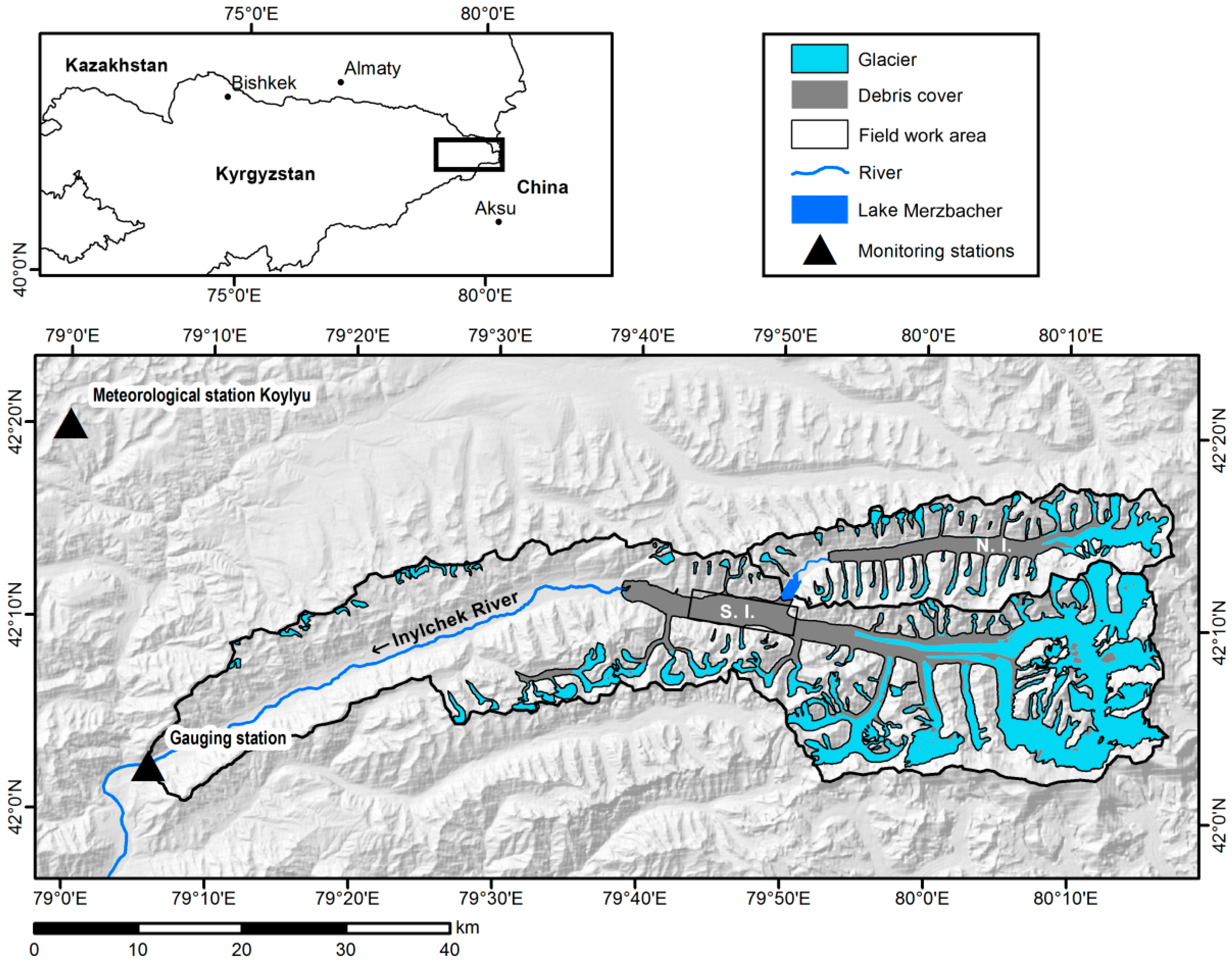
2.1. Study Area

The Inylchek glaciers are located in the Jengish Choqusu (Pobeda)-Khan Tengri massif in the Central Tian Shan (Figure 1), which is mainly built up by marine Paleozoic formations. These are folded schists, calcareous schists, siltstone and sandstone [48]. As a consequence, the clastic material of the moraines around and on the glaciers are weathered products of these metasediments. On such siliceous parent material develop acidic mountain soils that are generally poorly developed and skeletal. So-called leptosols are shallow and have a small water retention capacity, therefore they have a very small hydrological impact. In the Inylchek catchment, soils develop only on flat parts that were not glacier covered during the Little Ice Age.
The climate in the study area is generally continental with an amplitude of monthly air temperatures of around 30 K, but with increasing elevation, precipitation increases and temperature differences between summer and winter decrease [49]. At Koylyu meteorological station (2800 m a.s.l.) outside the catchment (Figure 1), annual mean temperature is −1.9 °C, with a minimum of −19.2 °C in January and a maximum of 10.3 °C in July. Westerlies from the Atlantic are the main source of humidity and the precipitation climate is mainly controlled by the interaction between the Siberian anticyclone during winter (dry conditions) and cyclonic activity from the west during summer (wet conditions). Thus, the Central Tian Shan experiences a distinct summer maximum of precipitation [49]. At Koylyu station, annual precipitation is 313 mm, 54% of which occurs in summer (Jun–Aug).
Located above the tree line, vegetation is limited to alpine tundra on a few lower and flatter locations of the catchment. Pioneer species like cushion plants exist in higher and steeper terrain, while in the snow zone no higher plants exist. Overall, vegetation is very scarce and transpiration can be neglected in the water cycle.
Until the second half of the 19th century, one joined, single Inylchek Glacier covered the Inylchek valley and its upper tributaries. Due to the warming trend following the Little Ice Age, the northern glacier part lost connection to the main part in the south and the glacier was separated into the Northern and the Southern Inylchek Glacier [50]; in the following called Northern and Southern Inylchek (Figure 1). Southern Inylchek acts as an ice dam towards the valley of Northern Inylchek and the runoff of Northern Inylchek is blocked. This water, together with calving ice from the dam, forms an ice-dammed lake called Lake Merzbacher. The lake has an approximate size of 4 km2 and a maximum depth of 100 m near the ice dam [51]. Lake Merzbacher empties nearly every year, causing a glacial lake outburst flood (GLOF), generally occurring in July or August.
Northern Inylchek experienced a surge in 1997 and slightly retreated again afterwards [53]. Today, Northern Inylchek covers an area of 152 km2, while Southern Inylchek has a glacier area of 418 km2. Their common catchment has a total area of about 800 km2 [54]. Both glaciers are heavily debris covered. The debris thickness ranges from a few millimeters up to several decimeters at the end of the glacier tongues. As at many debris-covered glaciers, the debris areas are interspersed with glacial-karst structures. The melt water of both glaciers forms Inylchek river, which drains into Sary-Dshaz river, the main tributary of Aksu river.

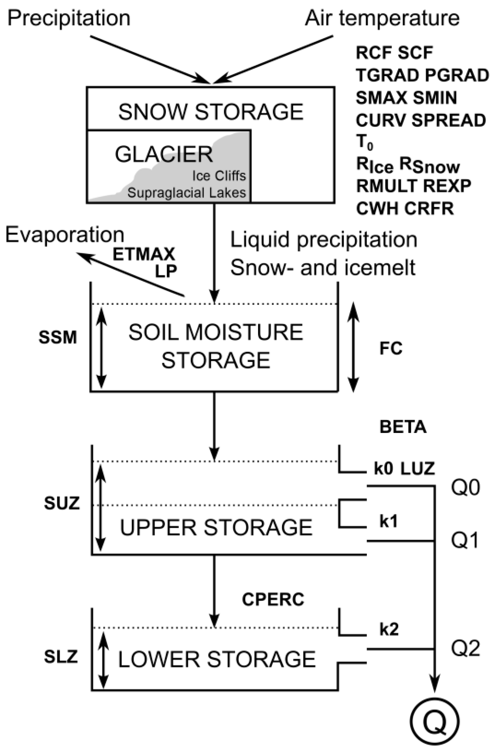
2.2. Hydrological Model

The HBV-LMU model used in this study is a raster-based temperature index model with a grid size of 180 × 180 m. It consists of four storages (Figure 2), is controlled by 23 free parameters (Table 1) and calculates accumulation, melt and runoff on a daily time step.
The model is based on the HBV3-ETH9 model version [55], which is a classic conceptual runoff model with a glacier routine that has been widely applied, also in Central Asia (e.g., Reference [23]). This general model approach was chosen because of its low data demand. Only precipitation and air temperature on a daily time step serve as input. Furthermore, the model showed a robust performance in earlier studies [20,21]. In order to reproduce sub-debris melt, the semi-distributed HBV-ETH has been set up partially distributed on a raster basis and was extended by several features. These are an automatic calibration procedure, allowing to introduce additional calibration criteria, and a routine to account for snow redistribution [56]. Finally, a routine to quantify melt below supraglacial debris, developed at Inylchek glaciers, has been implemented [47]. In this contribution, the calculation of melt at ice cliffs and supra-glacial lakes has also been included (see Section 2.2.2.) in the new model version (HBV-LMU). Owing to the special situation in the Inylchek catchment, the model also considers the buffering effect of Lake Merzbacher, but it cannot describe the outburst flood (see Section 2.2.4).

2.2.1. Spatially Distributed Surface Fluxes

Based on large-scale input fields of accumulation, the spatial variation is calculated according to Huss et al. [19]. Steep slope angles and convex curvatures diminish accumulation while at concave curvatures, accumulation is increased. This is controlled by the parameters CURV, SPREAD, SMIN and SMAX in the model.
Melt of snow and bare ice (MS, MBI) is calculated if the daily mean temperature (T) exceeds the threshold temperature (T0) based on an extended degree-day approach [57]. There, the degree-day factor is modified to consider shadowing and sun height at each grid cell. To do so, potential clear sky solar radiation (I) at every day and grid cell was calculated and added to the degree-day factor, which is now called melt factor MF, due to the modification. The relative influence is controlled individually for ice and snow areas using the parameters RSnow and RIce.
M S / BI =   { ( MF   +   R Snow / Ice   I )   ( T   - T 0 ) T   -   T 0   >   0 0 T   -   T 0     0
Snow melt infiltrates the remaining snow cover. The amount of stored water depends on the actual snow water equivalent and a parameter for water-holding capacity of snow (CWH). This water can refreeze and will be added to the snow cover if the daily mean temperature falls below T0, controlled by a refreezing coefficient (CRFR).

2.2.2. Ablation at Debris-Covered Areas, Ice Cliffs and Supraglacial Lakes

Ablation was measured at 26 ablation stakes from 14 July to 4 August 2012 in order to calculate empirical degree-day factors. Air temperature was recorded at a weather station located at the ice dam of Northern Inylchek close to Lake Merzbacher. Measured temperatures were extrapolated from the weather station located at the ice dam of Northern Inylchek to higher elevations using a lapse rate of 0.008 K m−1. This lapse rate has been determined by Han et al. [58] and is based on measurements at Koxkar glacier, which is also located in the Central Tian Shan. Ablation measurements were conducted similar to previous measurements at Koxkar Glacier [31].
The empirical relationship between debris cover thickness (DCT) and measured ablation was determined. The results are comparable to other studies [31,32,33,35]. Based on the relationship between DCT and ablation in dependence of the air temperature, the degree-day factors for debris-covered areas (DDFDI) are derived in two different ways, depending on the DCT. For very thin debris layers, increased melt is approximated by a linear function up to the thickness of maximum melt (in our case 0.0058 m, Equation (2)). This formula also provides the empirical degree-day factor for bare ice (DDFBI) for the case DCT = 0. For debris layers thicker than 5.8 mm, the degree-day factor is calculated by a power law regression (Equation (3)):
DDF DI / BI =   0.0953 × DCT + 0.0063   : DCT 5.8   mm ,
DDF DI =   DCT 0.3625 × 0.0011 : DCT > 5.8   mm .
The spatially distributed melt amount MDI (Equation (1)) is then determined by multiplying the potential bare ice melt MBI with the ratio of DDFDI to DDFBI at every grid cell:
M DI =   M BI × ( DDF DI DDF BI ) .  
Melt at ice cliffs was also determined by ablation stakes in 2012 and empirical degree-day factors to model melt at ice cliffs in three different aspects were calculated (DDF [m d−1 °C−1]: South: 0.0085, North: 0.0053 and East/West: 0.0071), assuming that the majority of ice cliffs have a characteristic slope. A similar ratio to the bare ice conditions as above was calculated for the ice cliff situation and scaled with the respective bare ice melt.
At supraglacial lakes, lateral melting and calving processes could not be considered in our model, because no parameterization of these processes are available. As melt rates at the bottoms of supraglacial lakes only depend on the debris’ thermal conductivity [41], they can be calculated based on the same relation of degree-day factor and DCT, assuming constant conductivity for the debris layer and a similar debris thickness in the lakes as in the debris-covered surroundings. In addition, a constant water temperature of 1 °C is considered [59].
Both ice cliffs and supraglacial lakes are mostly too small to be captured by the grid size of our model. For this reason, the percental areal share of ice cliffs and lakes to each grid cell was used as model input and considered for melt calculation.

2.2.3. Soil Moisture Storage and Runoff Generation

Melt water from snow and ice, as well as liquid precipitation, are summed up and form the hydrological input into the soil moisture routine (Figure 2). There, they fill the soil moisture storage (SSM). Loss due to evaporation from this storage was calculated based on the filling level of the storage and the potential evapotranspiration (ETpot) and a threshold value LP. ETpot is assumed if the SSM fill level exceeds the threshold LP. Infiltration of the remaining water into the upper storage was governed by SSM, the maximum soil storage capacity (FC) and a coefficient (BETA). From this upper storage, surface runoff (Q0) was calculated as soon as the storage filling level (SUZ) exceeded a threshold value (LUZ). The amount of Q0 is controlled by the parameter k0. Interflow from this storage was controlled by the filling level SUZ and the parameter k1. Constant infiltration into the lower storage was controlled by the parameter CPERC (see Table 1). Linear drainage from this storage was calculated based on its filling level SLZ and the parameter k2. The daily runoff of the catchment finally consists of the sum of the runoff volumes of Q0, Q1 and Q2.

2.2.4. Consideration of Lake Merzbacher
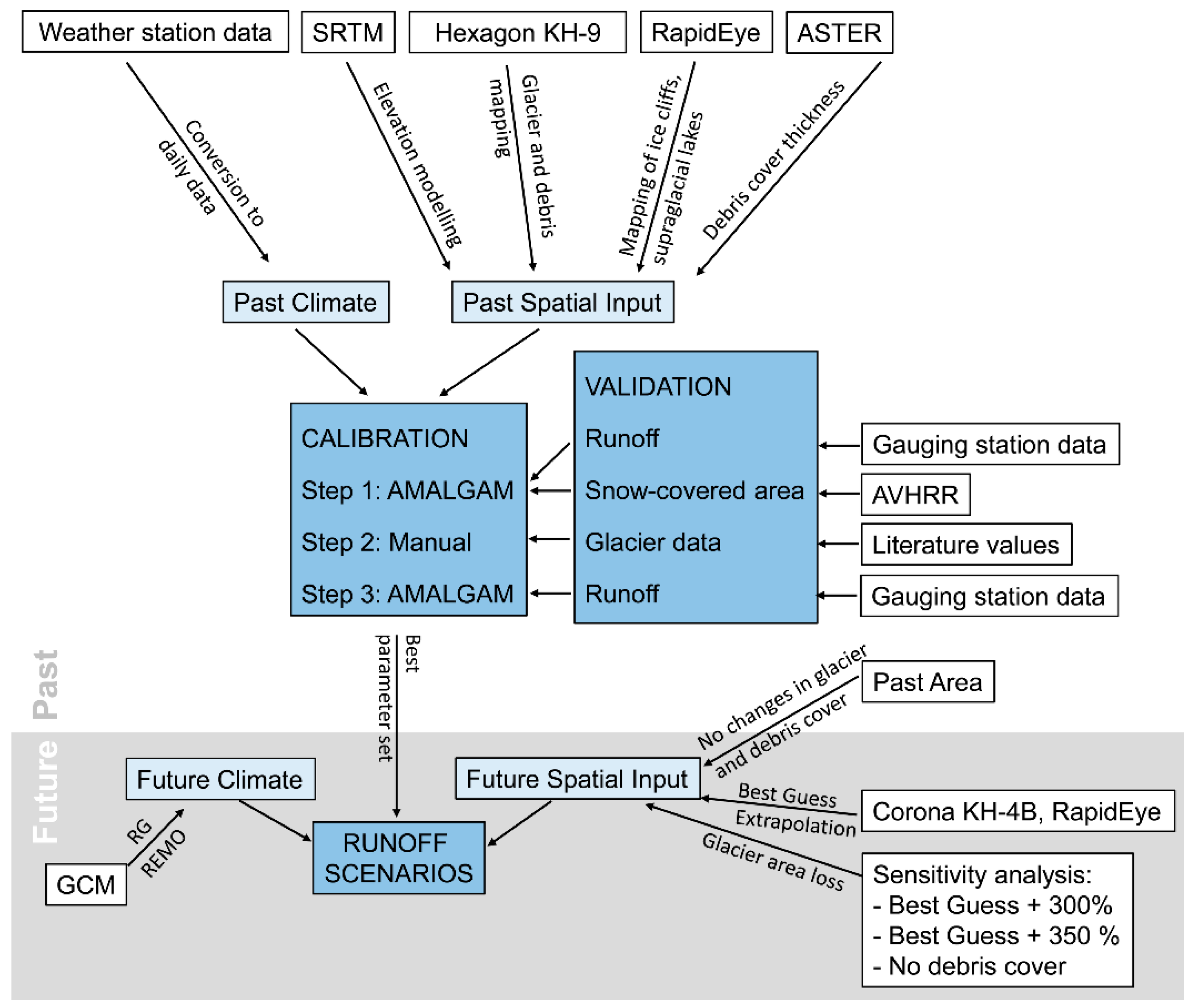
To simulate runoff at the Inylchek glaciers, it is necessary to consider the special catchment situation caused by Lake Merzbacher. First modelling attempts [54] revealed that, even in the phase of lake filling, the blocking ice dam is not a completely closed barrier. A permanent outflow from the lake needs to be considered by the model. In this study, this outflow is calculated based on the individual lake filling volume multiplied by an outflow variable. To determine this variable, individual calibration runs were conducted and the simulated lake filling volumes were compared to outburst volumes determined by Ng and Liu [60], for more details see Mayr et al. [54]. This revealed a best fitting daily drainage of 0.35% of the actual lake volume.

2.3. Input Data

2.3.1. Meteorological Input Data

Meteorological time series for air temperature and precipitation are available from Koylyu meteorological station (42°20′ N, 79°00′ E, elevation 2800 m a.s.l.), which is located 47 km west of the glacier terminus [60] (Figure 1). This weather station provided a gapless record of precipitation, air temperature, air humidity, air pressure and wind speed from 1951–1990. Unfortunately, these data were available in time steps of 10 days only. Based on this, daily temperature data were obtained by downscaling of ERA40 reanalysis data [61] using the regional climate model REMO (“Regional Model”) [62] Version 2009. Precipitation from the ERA-40 reanalysis has not been taken into account because it is supposed to be of low quality, due to the low resolution of the underlying model in the topographically diverse terrain of Central Asia. Indeed, the comparison between 10-days precipitation time series from ERA-40 and available stations revealed large discrepancies in terms of mean, standard deviation and phase relationship (not shown). Instead, daily precipitation values were generated by a Markov Chain approach and a Gamma-Distribution [63]. The according 10-daily means were compared to the measured means and the daily data corrected accordingly using a Delta-T-approach under consideration of the generated dryness or wetness of the days. The so derived daily data were used for model calibration.
The virtual point precipitation at the weather station is extrapolated by the hydrological model to the catchment by vertical gradients. To account for the representativeness of the weather station, the model implies calibrated correction factors for liquid and solid precipitation. This is standard procedure to create basin precipitation in conceptual runoff models. However, the so derived precipitation is subject to large uncertainties. Especially in glacierized catchments, where runoff can be generated by both precipitation and glacier melt, the danger of error compensation occurs if the model is calibrated by runoff only. In such a case, runoff simulations can show high efficiencies despite incorrect reproductions of precipitation and melt. For this reason, it is very important to use snow- and glacier related criteria for calibration and validation in order to constrain model parameters and thus reduce parameter uncertainty [64,65].
To simulate melt and runoff under past (1970/1971–1999/2000) and future (2070/2071–2099/2100) climate conditions, we generated meteorological input data using two different downscaling approaches: One dynamical approach using a regional climate model, and a statistical-dynamical approach. To keep results comparable, the ECHAM5/MPI-OM global climate model [66,67] has been used as boundary condition for both downscaling approaches. The choice of this GCM has been motivated by the fact that, at the time of producing the meteorological input, it was the climate model with highest spatial and temporal resolution provided via the CERA database and it still is a well evaluated global climate model for the Central Asian target region [16,68].
For the dynamical downscaling approach, we use the regional climate model REMO [62]. For reasons of limited computational resources, we could realize only one long-term climate change projection with REMO using the moderate A1B emission scenario. It represents an intermediate pathway of future climate change within the bunch of more recent RCP scenarios and is still often used for climate change studies. The resulting regional climate model data was bias corrected based on station data, using a linear correction for temperature [69] and a distribution derived transformation using the Gamma-distribution for precipitation [70]. In the following, these data are referred to as “REMO”.
For the statistical-dynamical methodology a circulation weather type (CWT) approach following Jones et al. [71] is utilized. This approach is applied to reanalysis (for calibration only) and GCM data in order to classify the daily lower-level atmospheric characteristics using 700 hPa geopotential height (GPH) fields as an input (for details, see Reference [17]). For future decades the three SRES scenarios B1 (optimistic, CO2 concentration increase from 367 ppm in the year 2000 to 540 ppm in 2100), A1B (moderate, 367 ppm to 703 ppm), and A2 (pessimistic, 367 ppm to 836 ppm) are considered. For each scenario three realizations are available. The statistical moments (e.g., mean and standard deviation) of the temperature and precipitation distribution were calculated for each CWT and season independently. To obtain continuous meteorological time series a random number generator (RNG) was used to generate temperature and precipitation time series that correspond to the statistical moments that were calculated for each CWT and season. Finally, the generated time series were recombined and weighted with the frequency of occurrence of each CWT [17]. To generate time series of precipitation and temperature from global climate projections, only the frequency of occurrence of each CWT was considered. Thus, this approach provides an estimate of the lower bound of possible changes in temperature and precipitation over this region as it does not consider possible changes of rainfall and temperature within the CWTs. These datasets are referred to as “RG” (for random generator) with their SRES scenario (e.g., RGB1, RGA1B and RGA2) in the following.
The downscaled meteorological input for the hydrological model does not arise from a multi-GCM multi-RCM ensemble approach. However, uncertainty of past and future meteorological boundary conditions is imposed by the two different downscaling approaches (dynamical versus statistical-dynamical) and by the statistical assessment in the framework of model data post-processing (see above), replacing the ensemble technique to a certain extent. In addition, scenario uncertainty is introduced by considering three different emission scenarios within the RG methodology.

2.3.2. Calibration Data

Runoff was measured at the gauging station near Inylchek village, 50 km downstream of the glacier snout (Figure 1) in the summer months of 1962–1965 and 1980–1981. The low flow winter period was not recorded and was therefore estimated manually by linear interpolation [47]. For model calibration, both, meteorological and runoff data are necessary, limiting the calibration years to 1963/1964, 1964/1965, and 1980/1981.
Snow cover information was extracted from Level 1b data of the Advanced Very High Resolution Radiometer (AVHRR) onboard the NOAA-9 satellite with a spatial resolution of 1100 m. If more than 50% of the model pixels inside one (non-) snow-covered AVHRR pixel were also (non-) snow-covered, this AVHRR pixel was counted as correctly attributed. The accuracy of snow cover classification from AVHRR is discussed in detail in Peters et al. [72]. They found a true positive rate of 87% between classified and directly observed snow in the Aksu basin. We chose seven images between April and September 1986 for our analyses, because 1986 was the only year with AVHRR and meteorological data coverage. The raw AVHRR images have to be pre-processed prior to snow cover extraction. This includes radiometric calibration and calculation of albedo and radiances, as well as the correction of sensor degradation and non-linearities in the measurements. Additionally, the images were geometrically rectified and referenced to UTM. The calibrated and referenced images were classified into the classes “snow”, “no snow”, and “clouds” using a dichotomous multi-channel classification scheme [73]. The model relies on surface temperature, albedo and NDVI to separate the classes. The thresholds of the subsequent steps were adapted to seasonal characteristics to improve accuracy. Cloud coverage has been reduced by employing a modified version of the Modsnow cloud removal algorithm [74].

2.3.3. Validation Values from Literature

Several glaciological studies have already been conducted at the Inylchek glaciers, their results could partly be used for model validation (Table 4). Aizen et al. [75] determined the mean mass balance at an elevation of 6147 m a.s.l and the equilibrium line altitude (ELA) for the years 1969–1989. Regional mass balances were calculated for the Inylchek glaciers based on surface elevation changes derived from multi-temporal digital terrain models (DTMs) [11] and ice transport rates [54]. For more details about the calculation see Mayr et al. [47].

2.3.4. Spatial Input

The model requires spatial information about glacier area, debris area, debris thickness, as well as the distribution of ice cliffs and supraglacial lakes. These elements may change over time, especially in a changing climate [42,76,77]. For the model calibration period and the past period 1971–2000, different sources of remote sensing data were used to generate the model input “Past Area” while for the future, a model input with possible changes was calculated, called “Best Guess” in the following. Additionally, three more glacier surface conditions were created to conduct a sensitivity analysis.
● Spatial input data for calibration period and past period (“Past Area”)
The glacier area and the debris-covered glacier part were manually delineated based on Hexagon KH-9 data from 1974 [11].
DCT was estimated by an empirical approach using thermal satellite imagery and local debris thickness measurements [31]. Measurements are available for 13 locations along a longitudinal profile (elevation from 3200 to 3300 m a.s.l.) in 2013. Land surface temperature (LST) was obtained following the approach by Pi et al. [78], using ASTER (Advanced Spaceborne Thermal Emission and Reflection Radiometer) Level 1B granule images of 12 May 2007. These data have a ground resolution of 30 m, they have been resampled to 180 m to match the model resolution. Mihalcea et al. [79] observed a strong correlation between ASTER-derived LST and debris thickness. Furthermore, in this study, debris thickness measurements in 25 pixels of the ASTER image showed a good correlation with surface temperature, thus LST could be used to estimate debris thickness distribution.
Ice cliffs and supraglacial lakes were mapped manually using a RapidEye image from 2011 [80]. According to the product specifications, RapidEye images have a positional accuracy of less than 10 m. This is more than enough for our purpose, where the absolute position of the features is not that important. Ice cliffs were differentiated into north, south and east/west facing cliffs. For melt calculation, the actual cliff area had to be calculated based on this horizontal data. Sakai et al. [41] found a range of ice cliff angles between 30° and 60° at Lirung Glacier. Therefore, a standard slope angle of 45° was used here [33].
Debris distribution, as well as ice cliff mapping, was performed using more recent remote sensing data compared to the calibration period. A comparison of the two periods revealed only minor changes in debris area and ice cliff distribution. Lakes seem to be slightly more numerous in 2011. This variation has very probably only a small impact on the melt calculation, because the lakes cover only 0.24% of the total glacier area in 2011.
● Spatial input data for future period (“Best Guess”)
Glaciers in the Tian Shan lost both area and mass during the last decades [10,81,82,83,84]. The major reason for the ice loss can be attributed to increasing air temperatures and changes in precipitation portioning [81,84]. Because increasing temperatures in the future will further enhance ice and snow melt, glacier area and mass are also expected to further decrease. Additionally, intensified melt and reduced ice flux increases the debris-covered area extent [85,86]. For this reason, the available spatial data had to be adapted for the projection period from 2071 to 2100.
To adapt the debris cover, we followed the approach of Jouvet et al. [87] and compared the RapidEye image from 2011 with a Corona KH-4B scene from August 1967 [88]. The KH-4B image was orthorectified using Remote Sensing Software Package Graz Version 7.46 with an RMS-X of 4.67 px and a RMS-Y of 4.02 px. The observed rate of debris front propagation was used to calculate a possible debris cover in 2085, as the middle of the 30 years’ future period. The influence of a possible increase of negative mass balances in the future was not considered. For this reason, the debris expansion might be slightly underestimated.
To adjust debris cover thickness, the following assumptions were made: Anderson [85] postulates that medial moraines show a relatively uniform debris thickness of only a few centimeters. The moraine widths increase downstream, but the thickness is relatively constant. Debris thickness starts to increase in areas where the moraines merge. Furthermore, at Inylchek, it is visible that debris at the moraine margins tends to be slightly thinner than in the middle. Based on these assumptions, new debris-covered areas were set to the mean debris thickness of the adjacent former marginal pixels. At these pixels, the debris thickness is supposed to increase. Their new debris thickness was calculated as the mean of their former debris thickness and the adjacent non-boundary pixels.
Volume changes of debris-covered glaciers are not reflected by variations of the glacier fronts, which commonly reveal a very stable behavior [89]. For this reason, the usual methods for glacier area adaption like the accumulation-area-ratio method [90] cannot be applied at debris-covered glaciers. To estimate the potential future glacier area, we used a similar method as for debris cover evolution. Consequently, images from 1967 (Corona KH-4B) and 2011 (RapidEye) were compared to identify the area decrease for 100 m elevation bands. To take a future atmospheric warming into account, a linear equation was derived based on these measurements and the ELA (4400 m to 4500 m) [75] as level with no area loss. To calculate the future glacier area, the ELA was shifted upwards. Model simulations performed during this study using the original glacier area under future climate conditions revealed that the ELA will increase up to 5300 m. The mean between the old ELA of 4400 m and the new one was used as mean ELA of our calculations. Based on this, it was possible to calculate the future area losses based on the previously mentioned equation. This approach results in a glacier area reduction of 22.5%.
● Spatial input data for sensitivity analysis
As first modelling results revealed that runoff will still increase with reduced glacier area, we decided to conduct a sensitivity analysis and generated three more glacier inputs. First and second, the areal loss of the above explained “Best Guess” input was increased by 300% and 350% respectively, leading to area reductions of 40.9% and 43.0%. Third, in order to analyze the effect of the debris cover on ice melt Northern and Southern Inylchek, we generated a hypothetical glacier extent without debris cover, ice cliffs and supraglacial lakes based on the glacier area of the Best Guess.

2.4. Model Calibration and Validation

To calibrate conceptual hydrological models, automatic calibration algorithms are frequently used [91]. One very promising approach is the multi-algorithm, genetically adaptive method (AMALGAM) of Vrugt and Robinson [92]. This algorithm was already successfully applied for the calibration of hydrological models [47,93].
To obtain valid calibration results, the multi-objective calibration approach is established. Additional to runoff, other measured data, such as seasonal and annual mass balances, are used for calibration. The simulation quality is assessed by the difference between measured and simulated data, the so called “objective functions”. The multi-objective approach usually leads to a reduced quality of runoff simulation, but better mass balance simulation [19,56,65,94,95]. If mass balance data are not available, snow cover from remote sensing imagery (e.g., MODIS, AVHRR) can be used as additional calibration dataset [96,97,98].

2.4.1. Objective Functions

The three years with all necessary data for model calibration were divided into differential split samples of two calibration years and one validation year [99,100]. In the following, these are called Sample 1, Sample 2 and Sample 3.
Runoff can be evaluated using the Nash-Sutcliffe coefficient (R2) and the volume error ratio (VER). Only runoff data prior to the onset of the GLOF of Merzbacher Lake were used for the calculation:
R 2 = 1   i = 1 n ( Q m Q s ) 2 i = 1 n ( Q m Q m ¯ ) 2 ,
  VER = abs ( ( i = 1 n Q s   i = 1 n Q m ) i = 1 n Q m )   × 100 ,  
where n is the total number of calculated time steps, Qm [m3 s−1] is the observed discharge and Qs [m3 s−1] is the simulated discharge.
The objective function snow-covered area (SCA) is calculated as the percentage of correctly attributed snow-covered and snow-free pixels (pxcorr) in the total number of pixels in the catchment (pxtot):
SCA = px corr px tot × 100.
As only one year of SCA data was available, it was used in each of the split samples.

2.4.2. Calibration Procedure

The quite complex arrangement of data and model inputs during the different steps of model application in the past and the future is summarized graphically in Figure 3.
At the first calibration step, the number of free model parameters (Table 1) is reduced from 23 to 19 by fixing the less sensitive parameters to reasonable values [54,56]. The automatic calibration procedure considered runoff (R2) and SCA (%). The most promising parameter set of each split sample was selected, called compromise solution in the following [101].
Although runoff and snow cover could be simulated very satisfactory (see Section 3.2. for details) in the first step, the modelled glacier mass balances were far too negative when compared to values from the literature (see Table 4). As this deviation could not be avoided by automatic calibration, we conducted a manual optimization run as a second calibration step. Here, we changed the parameters that control liquid precipitation and glacier mass balance in order to obtain more realistic mass losses. The other model parameters remained unchanged.
As a third calibration step, another automatic calibration run involving only the runoff parameters has been performed. In this step, the runoff simulation is optimized again under the changed precipitation and glacier mass regime. By fixing the other parameters, we force the model to find another optimum in a neighborhood with realistic glacier mass balances.

3. Results

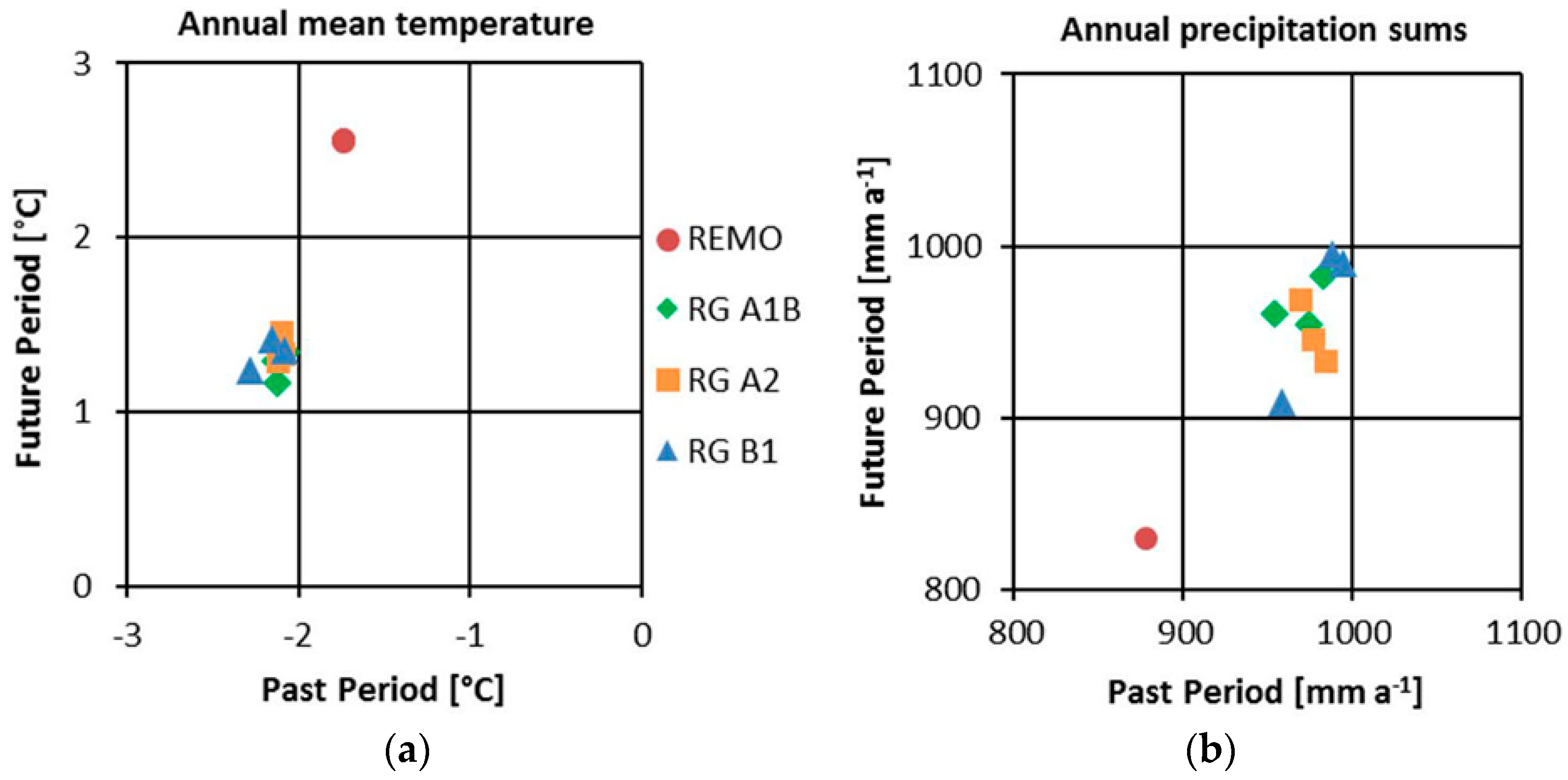
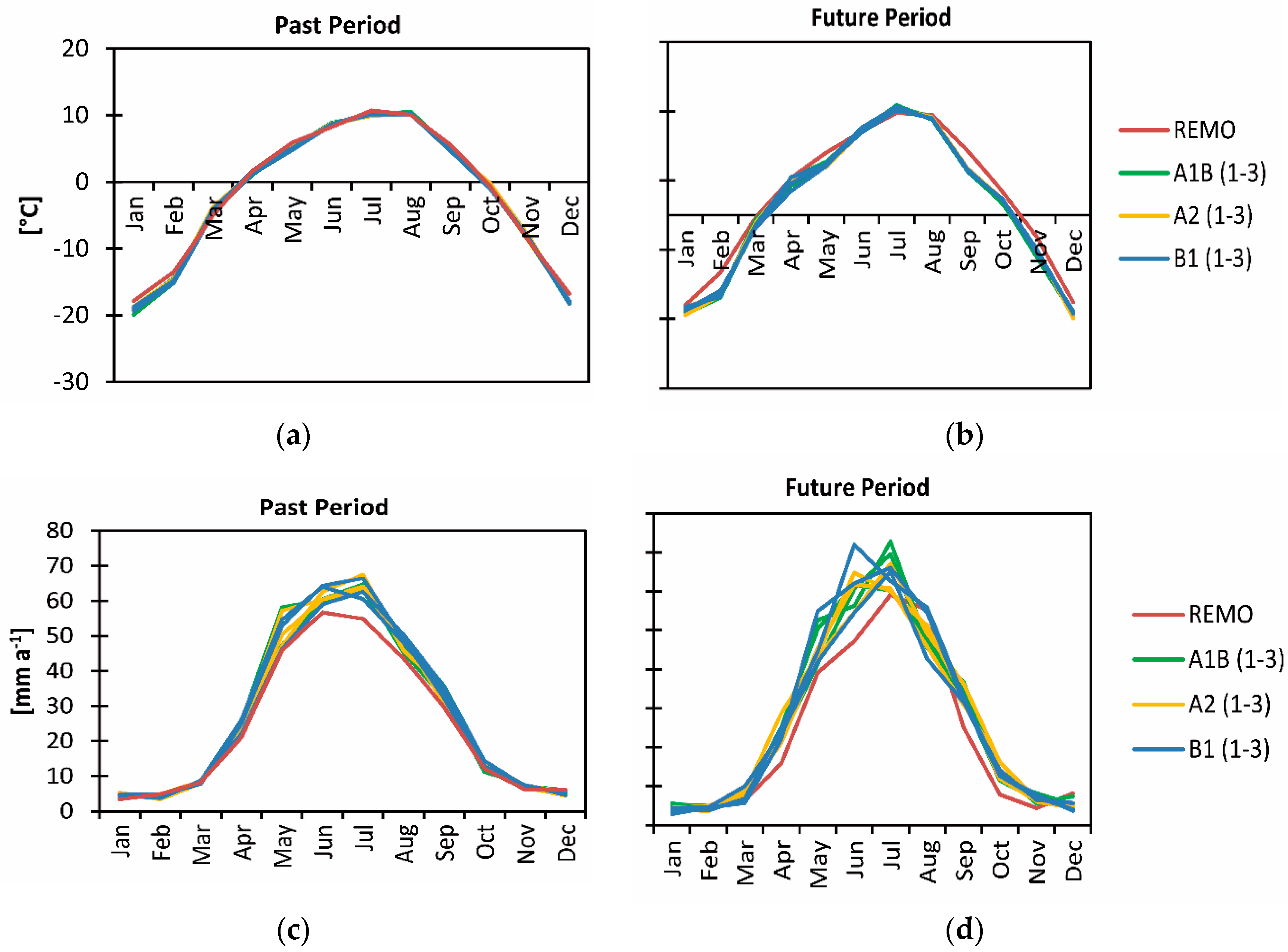
3.1. Climate Scenarios

The results of the climate models are visualized in Figure 4 (annual changes) and Figure 5 (monthly changes).
Temperature and precipitation of the REMO and RG scenarios differ considerably (Figure 4, Table 2). For the RG scenarios, the changes compared to past climate conditions are smaller than for REMO, as this approach only provides a lower bound of the possible changes of temperature and precipitation in this region. While precipitation decreases considerably in the REMO projections, the RG projections do not show a clear precipitation trend, though the majority of the RG projections simulate less precipitation for the future climate. Generally, differences between the three RG scenarios are rather small. For temperature, the magnitude of change is also highest for the REMO projections. However, both approaches reveal a strong warming for the future climate. The variations between the RG realizations partly covers the temperature differences between the scenarios, but they generally lie close together. Compared to the RG projections, the REMO scenario is warmer and dryer in the past period and this effect is further enhanced in the future period.

3.2. Calibration Results

During the first calibration step (automatic calibration) using the objective functions R2 and SCA, the three split samples converged to nearly stable values within 20,000 model evaluations. All Pareto fronts show small trade-offs in comparable ranges for both objective functions. Nash-Sutcliffe coefficients range from 0.71 to 0.94 and SCA range from 76 to 85.5% of pixels with correct assignment to snow-covered and snow-free areas. Based on this calibration, a compromise solution for each sample was chosen (Table 3).
Model runs over longer time periods using the selected compromise solution showed that local and overall mass balances are simulated far too negative in the ablation zone and not positive enough in the accumulation area (Table 4). This indicates that underestimated precipitation was compensated by overestimated melt rates. This error compensation has been reversed by the second calibration step, where the corresponding parameters were tuned manually. This second step improved glacier mass balances significantly, but reduced the quality of the runoff simulation.
The third step should optimize runoff as much as possible, without losing the realistic glacier mass balance values. For this purpose, another automatic calibration run only considering the runoff routine was conducted. Again, the objective functions R2 and VER were used. After 20,000 model evaluations, runoff is realistically simulated with Nash-Sutcliffe coefficients above 0.85 and VER of maximum 13% for the calibration year (Table 3), while the calculated mass balances remain within the range reported in the literature (Table 4). The snow-covered area is still well simulated with more than 82% of pixels with correct assignment to snow-covered and snow-free areas.

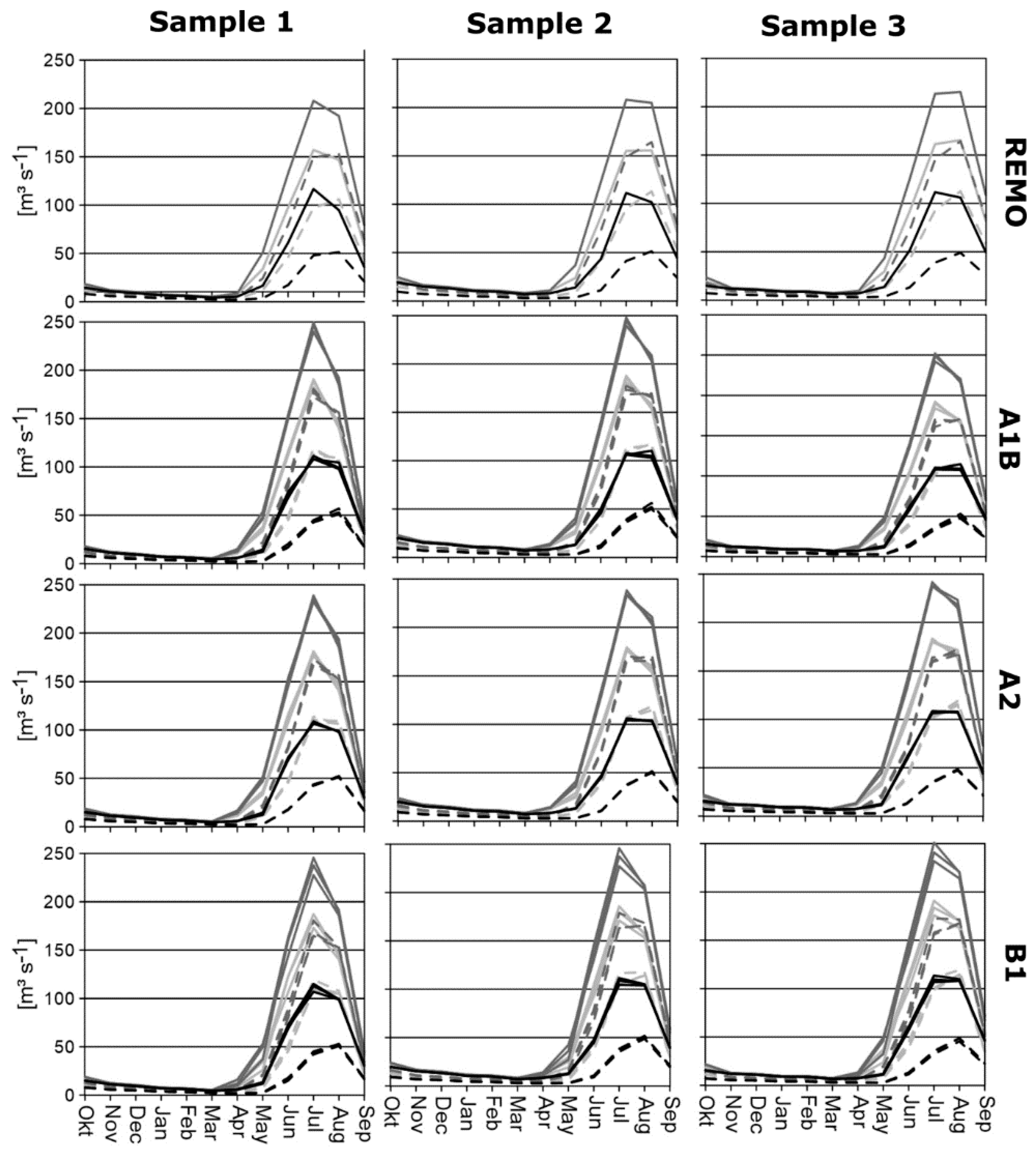
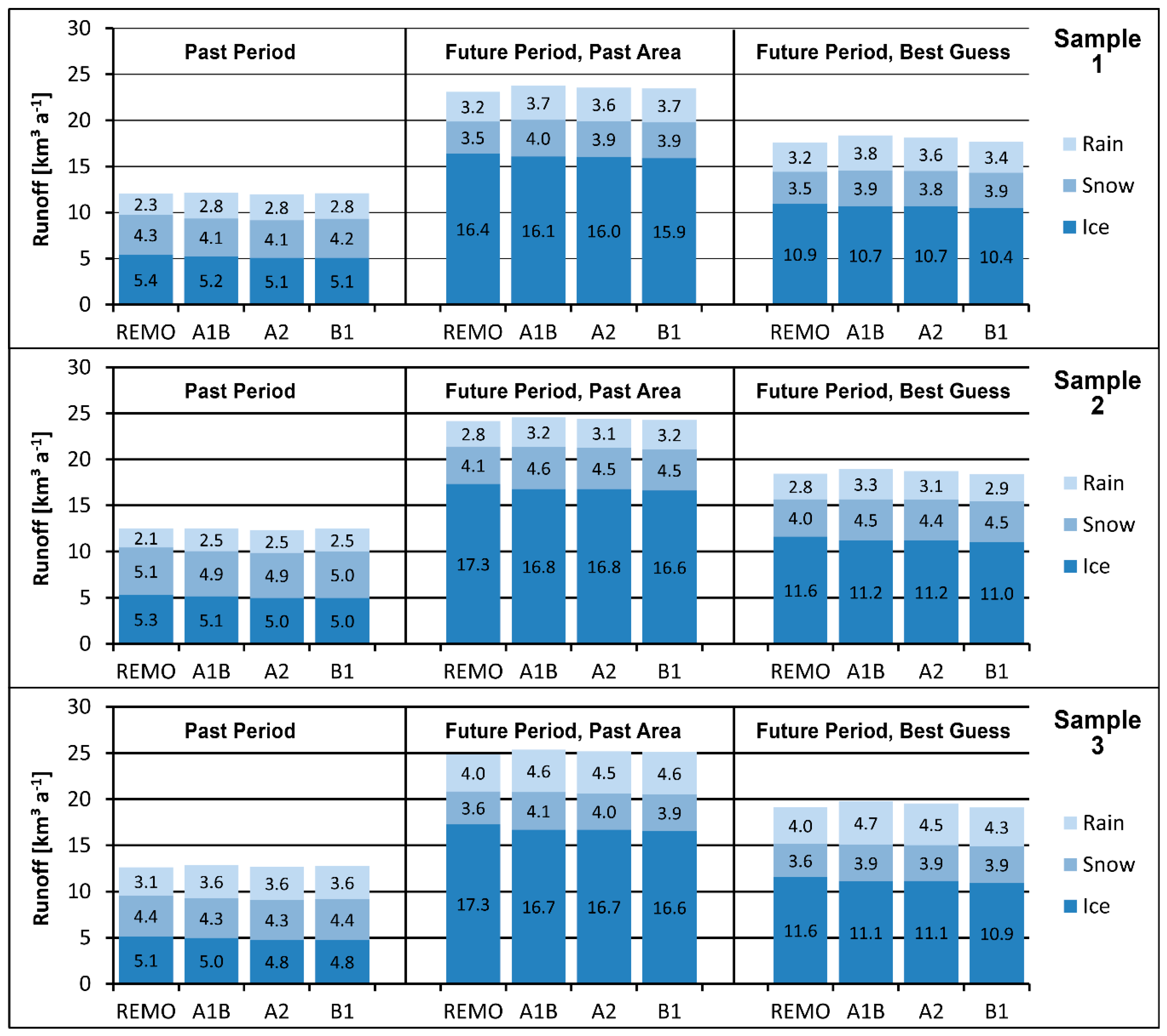
3.3. Melt- and Runoff Scenarios

We used the Compromise Solution parameter sets of the three split samples to simulate runoff for the Past and Future Periods. The Past Period was simulated with the Past Area as a model input, the Future Period was simulated with Past Area and Best Guess. Additionally, the model inputs of the sensitivity analysis were used. The main results are summarized in Table 5.
Compared to the Past Period, the runoff sums increase significantly in the future (Table 5). Since the three realizations of the RG scenarios differ only by standard deviations of 0 to 3%, only their means are presented here. If the past glacier area is assumed, the runoff nearly doubles, with an increase of 91% for REMO and up to 97% for the RG scenario A2. Using the Best Guess model input, runoff still increases, but in smaller ranges between 46% and 54% with a similar ranking of the scenarios. Using the model inputs of the sensitivity analysis, an area reduction of 40.9% still leads to a slightly increased runoff. If the glacier area is reduced by 43.0%, this leads to similar runoff as calculated in Period 1. This means that an area reduction of more than 43.0% is needed to compensate enhanced melt rates in the future climate. After this tipping point, further area recession will cause a reduction of annual discharge.
The mean monthly runoff and ice melt of all scenarios is presented in Figure 6. Due to higher deviations, especially in the spring months from April to June, all realizations of the RG scenarios are presented. In the Past Period, all samples and all scenarios show, more or less, the same runoff characteristics. The gradual decrease of runoff in the winter months stops with a small increase in May, followed by a more significant increase in June and runoff maxima in July and August. The individual runoff curves are controlled by both, the split sample and the climate scenario. Generally spoken, Sample 1 tends to produce runoff peaks in July, but more distinct for the REMO than for the RG scenarios. Sample 2 and 3 show a less distinct runoff peak in July, RG scenarios even show a double peak in July and August. For the Future Period (both, Past Area and Best Guess) and all scenarios and samples, the first runoff increase is now visible in April. This effect is strongest for the scenario A2 and smallest for REMO. In the REMO sets, the runoff peak in July is less distinct or even shifted to August, while for all RG scenarios the runoff peak in July is much more pronounced. In general, the runoff curves of the original and adapted area only differ in runoff amounts, but not in their distribution.
The differentiation of runoff into its sources rain, snow and ice is shown in Figure 7. In the Past Period, the biggest part of runoff is provided by ice melt, closely followed by snow melt and rain. Highest ice melt was simulated in all Periods by REMO and lowest by RG B1. At Sample 3, more rain and less snow melt are simulated compared to the other samples. In the future periods, ice melt increases considerably while snowmelt decreases and rain increases slightly. As expected, due to the smaller glacier area, the future period with adapted area shows smaller shares of ice melt.
The mean elevation of the ELA ranges from 5210 m a.s.l. in Sample 3 in RG Scenario A2 up to 5283m a.s.l. in Sample 2 at the REMO Scenario (Table 6).
The meltwater supplies of clean-ice areas, debris-covered areas and ice cliffs were exemplarily calculated for the past period of the REMO scenario with the Sample 1 parameter set (Table 7). The percental share of melt below debris is higher than its share of the total glacier area. Ice cliffs only contribute with slightly less than 5% to total ice melt, which is more than six times their areal share. The runoff contribution of ice melt at supraglacial lakes is even smaller than its areal share.
As shown in Table 4, regional and total mass balances were simulated satisfactory after the third calibration step. Additional to this calculation, the mass balance calculation using the fictional glacier input without debris cover, ice cliffs and supraglacial lakes are shown in Table 4 (grey shaded mass balance values). For this fictional clean-ice glacier, significantly higher mass losses are simulated for both, regional and overall mass balances.

4. Discussion

As confirmed already by several authors [97,98], SCA can be used successfully as objective function for model calibration. Here, the SCA simulation is considerably improved and the runoff simulation only slightly deteriorated compared to a calibration using runoff only. Duethmann et al. [98] recommend the use of SCA to obtain higher internal model consistency. In our study, this statement was verified using the validation values from the literature (Table 4). In fact, SCA helps to obtain better results for the ELA, which is simulated more realistically compared to model calibrations with runoff only. However, contrary to expectations, this does not automatically lead to better mass balance simulations. The model still provided too much runoff originating from snow and ice melt. This was also observed in an earlier study [23], where the HBV model underestimated basin precipitation and compensated this by overestimating glacier melt.
Manual parameter adjustment considering values from the literature seems to be a good opportunity to improve automatic calibration results. This procedure combines the advantages of both, automatic and manual calibration and can also be used if only soft data or expert knowledge is available [102]. The resulting deterioration of the runoff simulation could almost be eliminated by the second automatic calibration run for runoff improvement, where only parameters concerning runoff formation were changed.
The final Nash-Sutcliffe coefficients (R2) and volume error ratio (VER)m as well as snow-covered area (SCA) of the three split samples, lie generally within acceptable ranges compared to other studies with a multi-objective calibration approach (e.g., Reference [21]). While in Sample 1, the runoff curve of the validation year is simulated worse, this effect decreases in Samples 2 and 3. Similar results were found by Mayr et al. [54]. In sample two, the parameter set found in comparably wet years was capable to reproduce the hydrograph of a dry validation year. This is an indicator that the model calibration is also valid for simulations outside the rather short calibration period.
Results SCA simulations are slightly deteriorated during the manual refinement, but they are still much better as in model runs without consideration of SCA. Other studies [86,87,88] have calculated SCA not on a raster basis, but for elevation zones and therefore, their results cannot be compared directly.

4.1. How Will Runoff and Melt Change in Future?

Future runoff scenarios in glacierized catchments are generally hampered by high uncertainties [103]. The most important factors that determine the development of runoff characteristics over the next decades are future climate, future glacier size and future debris cover. All of them cannot be projected in a straightforward way, but have to be simulated or estimated by more or less complex models and assumptions. Another limitation is that we cannot be sure if the parametrization of the runoff model will still valid in a future climate. Although successful calibration and validation in separate years with different meteorological conditions gives some cause for optimism, our series of hydrometeorological data is too short to enable a real differential split-sample test after Klemes [99]. Being aware that our Best Guess is only one possible future, we are convinced that this future is a very likely one and that a more accurate projection is hardly possible with todays’ data and methods. Even if the magnitude of the hydrological response cannot be secured, we have confidence that trends and signals point into the right direction.

4.1.1. Annual Runoff Changes

Even with a glacier area reduction by 22.5%, the runoff will still increase significantly in the future. This is caused by higher melt rates in the ablation area due to higher temperatures, but also by the enlargement of the ablation area, due to the elevation shift of the ELA. A glacier area reduction of 43% is necessary to reduce runoff to the level of the Past Period. For the larger Aksu subbasins of Sari-Djaz and Kaksaal, Duethmann et al. [104] predict an overall increase in discharge for the period 2010–2039 (reference 1971–2000), but a decrease in 2070–2099 caused by an area reduction of 28–89% in the Sari-Djaz and 47–94% in the Kakshaal basin. Huss and Hock [105] also expect the runoff peak for the entire Tarim basin between 2030 (RCP2.6) and 2058 (RCP8.5) and thus a decline afterwards. These deviations from our results are due to the consideration of larger catchments with smaller degrees of glacierization, smaller average glacier size, and to a different methodology of estimating of future glacier extent, resulting in higher area losses.

4.1.2. ELA Changes

In our simulation, the ELA rises by about 800 m to elevations ranging from 5210 to 5283 m a.s.l., depending on sample and scenario. This increases the areal share of the ablation area from 49.9% to 87.9%, if the glacier area remains unchanged, and to 86.5% in case of the adapted area.
Modelling of the mass balance of Tian Shan glaciers until the end of the 21st century by Aizen et al. [106] revealed an mean increase of the equilibrium line altitude by 570 m and a decrease of the glacier covered area by 31%. Temperature is assumed to increase by 4 °C, which is comparable to our data. The deviation of ELA elevation is probably caused by the different assumptions on the precipitation trend, which is assumed to increase by 10% [106]. But even with a lower ELA, a smaller glacier area is assumed [106]. This clearly shows the high uncertainty of future glacier area assumptions. For this reason, we conducted a sensitivity analysis to identify the glacier coverage necessary for decreasing runoff.

4.1.3. Monthly Runoff Changes

Generally, the discharge hydrographs of the Past Period show a more or less pronounced runoff maximum in July and ice melt maximum in August. The hydrographs of the mean monthly runoff sums deviate only slightly in the different samples and scenarios (Figure 6). The most noticeable difference is the timing of the runoff peaks. Compared to RG, REMO has a lower June and higher July temperature, resulting in a melt-driven runoff peak in July. All samples of the scenarios show an ice melt maximum in August, because at this time, the ablation area is almost free of snow. Here, differences in the timing of runoff peaks can be explained by the used model parameters. For example, Sample 1 shows a higher runoff in July, combined with higher ice melt. Both are caused by a higher snow melt parameter Rsnow, which increases snow melt in July. The already snow-free glacier area increases the ice melt at the same time. Runoff in August is reduced, due to the already melted snow cover.
In the Future Period, the temperature increase in winter for the REMO scenario does not influence the melt rates because temperature remains below the melting point [8]. The earlier and more intense runoff in spring is caused by more intense snow melt, due to the overall higher spring temperatures, this effect was reported by many authors (e.g., by Hagg et al. [21] for the Rukhk catchment in the Pamir or by Akhtar et al. [107] for glaciers in the Hindukush-Karakorum-Himalaya region). In summer, the runoff curves changed differently for the REMO and RG scenarios. With REMO, the runoff peak in July is slightly lowered (Figure 6), because higher temperatures cause a shift of the snowmelt maximum from July to June. In contrast, the runoff peak in July is even more pronounced for the RG projections. The existing shift of snow melt is superimposed by an increase of ice melt in July, due to the temperature maximum in July in the RG scenarios. The deviations between the samples are similar to those of the Past Period. In general, the differences of runoff and ice melt between the different samples are relatively small. This supports the reliability of our modelling results.
Sorg et al. [83] suppose that continuing glacier mass losses in Tian Shan will finally lead to a change from glacial-nival to nival-pluvial runoff regimes, which will also increase the year-to-year variability of runoff. The timing of this change is highly dependent on the individual catchment and its glacier area development. This is not yet reached in our scenarios, as Northern and Southern Inylchek are comparatively large and therefore glacier melt still provides the main part of runoff.

4.2. What Is the Contribution of Snow, Ice and Precipitation to Runoff?

The share of ice melt in total runoff of the Past Period is 37–45%. Considering the high glacierization of more than 70%, this value seems small compared to the 36–38% calculated for the whole Aksu catchment (glacierization: 18%) by Aizen and Aizen [9]. In fact, these numbers cannot be compared properly, because Aizen and Aizen [9] consider all runoff from glaciers, including snow melt and liquid precipitation. It also should be noted that in very arid lowlands, the fraction of melt that is determined in the mountainous part of the basin, does not change anymore downstream. Comparing our findings to results from other catchments is even more difficult, because the fraction of ice melt strongly relies on climate. For example, the Rukhk catchment in the Pamir yields a significant share of ice melt of 32% with a glacier coverage of only 10%. This is caused by a very arid climate with an annual precipitation of only 295 mm [21]. In contrast, the Langtang Khola catchment in the Himalaya has glacier coverage of 43.5%, but the share of glacier runoff share was estimated to be only about 18%, due to its monsoon-influenced climate [108].
In the Future period, the share of ice melt increases significantly, due to the expected temperature increase. This warming will also cause more liquid precipitation, increasing the share of rain and decreasing snow melt. Enhanced ice melt will clearly overcompensate the decrease in glacier area and is expected to double until the end of this century. The timing of the tipping point, from which on area losses dominate and runoff decreases again, is mainly controlled by the initial glacier size and volume.

4.3. How Important Are Debris Cover, Ice Cliffs and Supraglacial Lakes for Melt Rates at Debris-Covered Glaciers?

Table 7 shows that the share of sub-debris melt in total runoff is higher than the fraction of debris covers in total glacier area. Since we assume that the presence of supraglacial debris causes an overall reduction of melt rates, this result may be surprising. It is caused by the fact that debris covers are situated at the lower parts of the glacier tongue, where air temperatures and resulting melt rates are higher than close to the equilibrium line, where bare ice dominates. The protecting effect of debris is confirmed by our test run using a fictional bare ice glacier (Table 4, grey shaded mass balance value). Here, simulated ice melt increases significantly compared to the original, debris-covered glacier. This supports the finding of Zhang et al. [32] at nearby Keqicar Baqi Glacier in the Chinese Tian Shan and Ragettli et al. [34] on debris-covered glaciers in the Langtang Himal, Nepal and conflicts with the results of other studies [36,37,38].
But even though thick debris covers have an insulating effect, considerable downwasting at heavily debris-covered glaciers has been observed, especially in parts which are interspersed with ice cliffs and supraglacial lakes [83,109,110]. The melt in supraglacial lakes is most likely underestimated in our results as lateral melt and calving could not be considered. The increased melt at ice cliffs, as stated by several authors [33,41,42,44,111] is confirmed by our findings (Table 7). Considering the small area covered by ice cliffs, their share in total ice melt is significant. However, according to our results, the enhanced ice melt at ice cliffs on Inylchek glaciers cannot compensate the overall isolating effect of the debris cover.

5. Conclusions

This study shows that additional objective functions, such as snow-covered area, improve the simulation quality of the respective variable, but do not guarantee valid model calibrations. Simulation results always need to be checked carefully on their plausibility, using available field data or expert knowledge. Considering these kinds of data during manual parameter adjustment is a good opportunity to improve automatic calibration results.
Using both, dynamical and statistical-dynamical modelling approaches to assess regional climate reveals significant projection differences. While the former estimates an upper bound for the possible changes in temperature and precipitation over the region, the latter provided a lower bound and considered multiple SRES scenarios, thus permitting an estimation of uncertainties. This emphasizes the need to meet uncertainties, due to climate modeling and the choice of the downscaling approach by including several downscaling realizations.
From 1970/1971 to 1999/2000, the share of ice melt in total runoff was 37–45%. By the end of this century, this already high share of ice melt, as well as total runoff, will still significantly increase, due to strongly enhanced ice melt in the warmer atmosphere and comparably small area losses of the heavily debris-covered Inylchek glaciers. As ice melt will still be the main source of runoff in this highly glacierized subbasin, a change from a glacial-nival to a nival-pluvial runoff regime will not be reached in this century according to our model results.
A major part of ice melt is provided by debris-covered glacier parts. This doesn’t contradict the assumption of a protecting effect of debris covers, but is caused by the spatial distribution of debris-covered and clean-ice glacier areas. Simulations at a fictional clean-ice glacier confirm the protecting effect of a debris cover. Compared to the original debris-covered glacier, ice melt is increased significantly if a clean ice surface is assumed.
At ice cliffs, melt is significantly increased, but it is not high enough to compensate for the isolating effect of the debris cover. Melt in supraglacial lakes is most likely underestimated because lateral melt and calving could not be considered in the model approach. These processes should be implemented into the model in the future in order to further improve predictions of water availability in this region.
Although the projected increase in runoff will counteract man-made water shortages downstream and probably mitigate the negative ecological impacts, one should keep in mind that the additional water yield from glacier wastage is preliminary and not of sustainable nature.

Author Contributions

Conceptualization, E.M. and W.H.; Methodology, H.P., C.M., W.H., T.B.; Software, E.M.; Data Curation, E.M., B.M., M.R., D.S., J.P., T.P., M.J.; Writing—Original Draft Preparation, W.H., E.M., B.M., M.R., D.S., J.G.P., J.P., T.P., T.B., H.P., C.M.; Writing—Review and Editing, W.H., C.M., T.B.; Visualization, E.M.; Supervision, W.H., C.M., H.P., T.B.; Project Administration, H.P.

Funding

This research was funded by the Deutsche Forschungsgemeinschaft (DFG) Bundle Project PAK 393 “AKSU-TARIM: Climate change and water resources in western China” (project Nos. 100434939, 100348997, 116182412, 112742139). During the preparation of the manuscript, Wilfried Hagg was supported by the DFG Heisenberg program (project No. 256557984). Joaquim G. Pinto received support from AXA research fund.

Acknowledgments

The German Research Centre for Geosciences (Geoforschungszentrum, GFZ) in Potsdam and the Central Asian Institute for Applied Geosciences (CAIAG) in Bishkek offered essential logistic help during the field campaigns. Gleb Glazirin, Tashkent, supplied important hydrometeorological data and Jasper Vrugt (University of California, Irvine) kindly provided his calibration algorithm. The comments of three anonymous reviewers are greatly acknowledged.

Conflicts of Interest

The authors declare no conflict of interest. The funders had no role in the design of the study; in the collection, analyses, or interpretation of data; in the writing of the manuscript, and in the decision to publish the results.

References

  1. Kaser, G.; Grosshauser, M.; Marzeion, B. Contribution potential of glaciers to water availability in different climate regimes. Proc. Natl. Acad. Sci. USA 2010, 107, 20223–20227. [Google Scholar] [CrossRef] [PubMed]
  2. Jiang, L.W. Water resources, land exploration and population dynamics in arid areas—The case of the Tarim River Basin in Xinjiang of China. Popul. Environ. 2005, 26, 471–503. [Google Scholar] [CrossRef]
  3. Feike, T.; Mamitimin, Y.; Li, L.; Doluschitz, R. Development of agricultural land and water use and its driving forces along the Aksu and Tarim River, PR China. Environ. Earth Sci. 2015, 73, 517–531. [Google Scholar] [CrossRef]
  4. Hou, P.; Beeton, R.; Carter, R.; Dong, X.; Li, X. Response to environmental flows in the lower Tarim River, Xinjiang, China: Ground water. J. Environ. Manag. 2007, 83, 371–382. [Google Scholar] [CrossRef] [PubMed]
  5. Xu, Z.; Chen, Y.; Li, J. Impact of climate change on water resources in the Tarim River basin. Water Resour. Manag. 2004, 18, 439–458. [Google Scholar] [CrossRef]
  6. Liu, Y.; Chen, Y. Impact of population growth and land-use change on water resources and ecosystems of the arid Tarim River Basin in Western China. Int. J. Sustain. Dev. World 2010, 13, 295–305. [Google Scholar] [CrossRef]
  7. Chen, Y.N.; Xu, C.C.; Hao, X.M.; Li, W.H.; Chen, Y.P.; Zhu, C.G.; Ye, Z.X. Fifty-year climate change and its effect on annual runoff in the Tarim River Basin, China. Quat. Int. 2009, 208, 53–61. [Google Scholar] [CrossRef]
  8. Kundzewicz, Z.; Merz, B.; Vorogushyn, S.; Hartmann, H.; Duethmann, D.; Wortmann, M.; Huang, S.; Su, B.; Jiang, T.; Krysanova, V. Analysis of changes in climate and river discharge with focus on seasonal runoff predictability in the Aksu River Basin. Environ. Earth Sci. 2015, 73, 501–516. [Google Scholar] [CrossRef]
  9. Aizen, V.B.; Aizen, E.M. Estimation of glacial runoff to the Tarim River, central Tien Shan. IAHS Publ. 1998, 248, 191–198. [Google Scholar]
  10. Pieczonka, T.; Bolch, T. Region-wide glacier mass budgets and area changes for the Central Tien Shan between 1975 and 1999 using Hexagon KH-9 imagery. Glob. Planet. Chang. 2015, 128, 1–13. [Google Scholar] [CrossRef]
  11. Shangguan, D.H.; Bolch, T.; Ding, Y.J.; Krohnert, M.; Pieczonka, T.; Wetzel, H.U.; Liu, S.Y. Mass changes of Southern and Northern Inylchek Glacier, Central Tian Shan, Kyrgyzstan, during similar to 1975 and 2007 derived from remote sensing data. Cryosphere 2015, 9, 703–717. [Google Scholar] [CrossRef]
  12. Liu, S.Y.; Ding, Y.J.; Shangguan, D.H.; Zhang, Y.; Li, J.; Han, H.D.; Wang, J.; Xie, C.W. Glacier retreat as a result of climate warming and increased precipitation in the Tarim river basin, northwest China. Ann. Glaciol. 2006, 43, 91–96. [Google Scholar] [CrossRef]
  13. Shangguan, D.; Liu, S.; Ding, Y.; Ding, L.; Xu, J.; Jing, L. Glacier changes during the last forty years in the Tarim Interior River basin, northwest China. Prog. Nat. Sci. 2009, 19, 727–732. [Google Scholar] [CrossRef]
  14. Osmonov, A.; Bolch, T.; Xi, C.; Kurban, A.; Guo, W. Glacier characteristics and changes in the Sary-Jaz River Basin (Central Tien Shan, Kyrgyzstan)–1990–2010. Remote. Sens. Lett. 2013, 4, 725–734. [Google Scholar] [CrossRef]
  15. Cruz, R.V.; Harasawa, H.; Lal, M.; Wu, S.; Anokhin, Y.; Punsalmaa, B.; Honda, Y.; Jafari, M.; Li, C.; Huu Ninh, N. Asia. In Climate Change 2007: Impacts, Adaptation and Vulnerability. Contribution of Working Group II to the Fourth Assessment Report of the Intergovernmental Panel on Climate Change; Parry, M.L., Canziani, O.F., Palutikof, J.P., van der Linden, P.J., Hanson, C.E., Eds.; Cambridge University Press: Cambridge, UK, 2007; pp. 469–506. [Google Scholar]
  16. Mannig, B.; Mueller, M.; Starke, E.; Merkenschlager, C.; Mao, W.; Zhi, X.; Podzun, R.; Jacob, D.; Paeth, H. Dynamical downscaling of climate change in Central Asia. Glob. Planet. Chang. 2013, 110, 26–39. [Google Scholar] [CrossRef]
  17. Reyers, M.; Pinto, J.G.; Paeth, H. Statistical-dynamical downscaling of present day and future precipitation regimes in the Aksu river catchment in Central Asia. Glob. Planet. Chang. 2013, 107, 36–49. [Google Scholar] [CrossRef]
  18. Konz, M.; Uhlenbrook, S.; Braun, L.; Shrestha, A.; Demuth, S. Implementation of a process-based catchment model in a poorly gauged, highly glacierized Himalayan headwater. Hydrol. Earth Syst. Sci. 2007, 11, 1323–1339. [Google Scholar] [CrossRef] [Green Version]
  19. Huss, M.; Farinotti, D.; Bauder, A.; Funk, M. Modelling runoff from highly glacierized alpine drainage basins in a changing climate. Hydrol. Process. 2008, 22, 3888–3902. [Google Scholar] [CrossRef]
  20. Shahgedanova, M.; Hagg, W.; Zacios, M.; Popovnin, V. An Assessment of the Recent Past and Future Climate Change, Glacier Retreat, and Runoff in the Caucasus Region Using Dynamical and Statistical Downscaling and HBV-ETH Hydrological Model. NATO Sci. Peace Secur. 2009, 63–72. [Google Scholar] [CrossRef]
  21. Hagg, W.; Hoelzle, M.; Wagner, S.; Mayr, E.; Klose, Z. Glacier and runoff changes in the Rukhk catchment, upper Amu-Darya basin until 2050. Glob. Planet. Chang. 2013, 110, 65–73. [Google Scholar] [CrossRef]
  22. Hagg, W.; Braun, L.N.; Weber, M.; Becht, M. Runoff modelling in glacierized Central Asian catchments for present-day and future climate. Nord. Hydrol. 2006, 37, 93–105. [Google Scholar] [CrossRef] [Green Version]
  23. Hagg, W.; Braun, L.; Kuhn, M.; Nesgaard, T. Modelling of hydrological response to climate change in glacierized Central Asian catchments. J. Hydrol. 2007, 332, 40–53. [Google Scholar] [CrossRef] [Green Version]
  24. Sorg, A.; Huss, M.; Rohrer, M.; Stoffel, M. The days of plenty might soon be over in glacierized Central Asian catchments. Environ. Res. Lett. 2014, 9, 104018. [Google Scholar] [CrossRef] [Green Version]
  25. Wortmann, M.; Krysanova, V.; Kundzewicz, Z.W.; Su, B.; Li, X. Assessing the influence of the Merzbacher Lake outburst floods on discharge using the hydrological model SWIM in the Aksu headwaters, Kyrgyzstan/NW China. Hydrol. Process. 2014, 28, 6337–6350. [Google Scholar] [CrossRef]
  26. Luo, Y.; Arnold, J.; Liu, S.; Wang, X.; Chen, X. Inclusion of glacier processes for distributed hydrological modeling at basin scale with application to a watershed in Tianshan Mountains, northwest China. J. Hydrol. 2013, 477, 72–85. [Google Scholar] [CrossRef]
  27. Bolch, T. Asian glaciers are a reliable water source. Nature 2017, 545, 161–162. [Google Scholar] [CrossRef] [PubMed]
  28. Scherler, D.; Bookhagen, B.; Strecker, M.R. Spatially variable response of Himalayan glaciers to climate change affected by debris cover. Nat. Geosci. 2011, 4, 156–159. [Google Scholar]
  29. Carenzo, M.; Pellicciotti, F.; Mabillard, J.; Reid, T.; Brock, B.W. An enhanced temperature index model for debris-covered glaciers accounting for thickness effect. Adv. Water Resour. 2016, 94, 457–469. [Google Scholar] [CrossRef] [PubMed]
  30. Østrem, G. Ice melting under a thin layer of moraine, and the existence of ice cores in moraine ridges. Geogr. Ann. A 1959, 41, 228–230. [Google Scholar] [CrossRef]
  31. Mihalcea, C.; Mayer, C.; Diolaiuti, G.; Lambrecht, A.; Smiraglia, C.; Tartari, G. Ice ablation and meteorolopical conditions on the debris-covered area of Baltoro glacier, Karakoram, Pakistan. Ann. Glaciol. 2006, 43, 292–300. [Google Scholar] [CrossRef]
  32. Zhang, Y.; Liu, S.Y.; Ding, Y.J. Glacier meltwater and runoff modelling, Keqicar Baqi glacier, Southwestern Tien Shan, China. J. Glaciol. 2007, 53, 91–98. [Google Scholar] [CrossRef]
  33. Juen, M.; Mayer, C.; Lambrecht, A.; Han, H.; Liu, S. Impact of varying debris cover thickness on ablation: A case study for Koxkar Glacier in the Tien Shan. Cryosphere 2014, 8, 377–386. [Google Scholar] [CrossRef] [Green Version]
  34. Ragettli, S.; Bolch, T.; Pellicciotti, F. Heterogeneous glacier thinning patterns over the last 40 years in Langtang Himal, Nepal. Cryosphere 2016, 10, 2075–2097. [Google Scholar] [CrossRef]
  35. Hagg, W.; Mayer, C.; Lambrecht, A.; Helm, A. Sub-debris melt rates on Southern Inylchek Glacier, Central Tian Shan. Geogr. Ann. A 2008, 90, 55–63. [Google Scholar] [CrossRef] [Green Version]
  36. Kääb, A.; Berthier, E.; Nuth, C.; Gardelle, J.; Arnaud, Y. Contrasting patterns of early twenty-first-century glacier mass change in the Himalayas. Nature 2012, 488, 495–498. [Google Scholar] [CrossRef] [PubMed]
  37. Nuimura, T.; Fujita, K.; Yamaguchi, S.; Sharma, R.R. Elevation changes of glaciers revealed by multitemporal digital elevation models calibrated by GPS survey in the Khumbu region, Nepal Himalaya, 1992–2008. J. Glaciol. 2012, 58, 648–656. [Google Scholar] [CrossRef]
  38. Gardelle, J.; Berthier, E.; Arnaud, Y.; Kääb, A. Region-wide glacier mass balances over the Pamir-Karakoram-Himalaya during 1999–2011. Cryosphere 2013, 7, 1263–1286. [Google Scholar] [CrossRef] [Green Version]
  39. Mavlyudov, B. Glacial karst, why it important to research. Acta Carsol. 2006, 35, 55–67. [Google Scholar] [CrossRef]
  40. Buri, P.; Pellicciotti, A. Aspect controls the survival of ice cliffs on debris-covered glaciers. Proc. Natl. Acad. Sci. USA 2018, 201713892. [Google Scholar] [CrossRef] [PubMed]
  41. Sakai, A.; Takeuchi, N.; Fujita, K.; Nakawo, M. Role of supraglacial ponds in the ablation process of a debris-covered glacier in the Nepal Himalayas, Debris-Covered Glaciers. IAHS Publ. 2000, 265, 119–130. [Google Scholar]
  42. Han, H.D.; Wang, J.A.; Wei, J.F.; Liu, S.Y. Backwasting rate on debris-covered Koxkar glacier, Tuomuer mountain, China. J. Glaciol. 2010, 56, 287–296. [Google Scholar] [CrossRef]
  43. Benn, D.I.; Bolch, T.; Hands, K.; Gulley, J.; Luckman, A.; Nicholson, L.I.; Quincey, D.; Thompson, S.; Toumi, R.; Wiseman, S. Response of debris-covered glaciers in the Mount Everest region to recent warming, and implications for outburst flood hazards. Earth-Sci. Rev. 2012, 114, 156–174. [Google Scholar] [CrossRef] [Green Version]
  44. Reid, T.D.; Brock, B.W. Assessing ice-cliff backwasting and its contribution to total ablation of debris-covered Miage glacier, Mont Blanc massif, Italy. J. Glaciol. 2014, 60, 3–13. [Google Scholar] [CrossRef] [Green Version]
  45. Sakai, A.; Nakawo, M.; Fujita, K. Distribution characteristics and energy balance of ice cliffs on debris-covered glaciers, Nepal Himalaya. Arct. Antarct. Alp. Res. 2002, 34, 12–19. [Google Scholar] [CrossRef]
  46. Benn, D.I.; Wiseman, S.; Hands, K.A. Growth and drainage of supraglacial lakes on debris-mantled Ngozumpa Glacier, Khumbu Himal, Nepal. J. Glaciol. 2001, 47, 626–638. [Google Scholar] [CrossRef]
  47. Mayr, E.; Juen, M.; Mayer, C.; Usubaliev, R.; Hagg, W. Modeling Runoff from the Inylchek Glaciers and Filling of Ice-Dammed Lake Merzbacher, Central Tian Shan. Geogr. Ann. A 2014, 96, 609–625. [Google Scholar] [CrossRef]
  48. Mikolaichuk, A.V.; Apayarov, F.K.; Chernavskaja, Z.I.; Skrinnik, L.I.; Ghes, M.D.; Neyevin, A.V.; Charimov, T.A. Geological Map of Khan-Tengri Massif—Explanatory Note; ISTC Project No. KR-920. Available online: http://www.kyrgyzstan.ethz.ch/fileadmin/download/kr920/explanatory_note_kr920.pdf (accessed on 22 October 2018).
  49. Aizen, V.B.; Aizen, E.M.; Melack, J.M. Climate snow cover, glaciers and runoff in the Tien Shan, Central Asia. Water Resour. Bull. 1995, 31, 1113–1129. [Google Scholar] [CrossRef]
  50. Glazirin, G.E.; Popov, V.I. Lednik Severnyi Inylchek za poslednie poltora veka [Northern Inylchek Glacier in the last 150 years]. Materialy Glyatsiologicheskikh Issledovannii (Data Glaciol. Stud.) 1999, 87, 165–168. (In Russian) [Google Scholar]
  51. Glazirin, G. A century of investigations on outbursts of the icedammed lake Merzbacher (central Tien Shan). Austr. J. Earth Sci. 2010, 103, 171–179. [Google Scholar]
  52. Jarvis, A.; Reuter, H.I.; Nelson, A.; Guevara, E. Hole-filled SRTM for the globe Version 4. The CGIAR-CSI SRTM 90 m Database. 2008. Available online: http://srtm.csi.cgiar.org (accessed on 7 November 2017).
  53. Mukherjee, K.; Bolch, T.; Goerlich, F.; Kutuzov, S.; Osmonov, A.; Pieczonka, T.; Shesterova, I. Surge-type glaciers in the Tien Shan (Central Asia). Arct. Antarct. Alp. Res. 2017, 49, 147–171. [Google Scholar] [CrossRef]
  54. Mayer, C.; Lambrecht, A.; Hagg, W.; Helm, A.; Scharrer, K. Post-drainage ice dam response at Lake Merzbacher, Inylchek glacier, Kyrgyzstan. Geogr. Ann. A 2008, 90, 87–96. [Google Scholar] [CrossRef]
  55. Braun, L.; Weber, M.; Schulz, M. Consequences of climate change for runoff from Alpine regions. Ann. Glaciol. 2000, 31, 19–25. [Google Scholar] [CrossRef]
  56. Mayr, E.; Hagg, W.; Mayer, C.; Braun, L. Calibrating a spatially distributed conceptual hydrological model using runoff, annual mass balance and winter mass balance. J. Hydrol. 2013, 478, 40–49. [Google Scholar] [CrossRef]
  57. Hock, R. A distributed temperature-index ice- and snowmelt model including potential direct solar radiation. J. Glaciol. 1999, 45, 101–111. [Google Scholar] [CrossRef] [Green Version]
  58. Han, H.; Liu, S.; Ding, Y.; Deng, X.; Wang, Q.; Xie, C.; Wang, J.; Zhang, Y.; Li, J.; Shangguan, D.; et al. Near-surface meteorological characteristics on the Koxkar Baxi Glacier, Tianshan. J. Glaciol. Geocryol. 2008, 30, 967–975. [Google Scholar]
  59. Roehl, K. Characteristics and evolution of supraglacial ponds on debris-covered Tasman Glacier, New Zealand. J. Glaciol. 2008, 54, 867–880. [Google Scholar] [CrossRef] [Green Version]
  60. Ng, F.; Liu, S. Temporal dynamics of a jokulhlaup system. J. Glaciol. 2009, 55, 651–665. [Google Scholar] [CrossRef]
  61. Uppala, S.M.; Kallberg, P.W.; Simmons, A.J.; Andrae, U.; Bechtold, V.D.; Fiorino, M.; Gibson, J.K.; Haseler, J.; Hernandez, A.; Kelly, G.A.; et al. The ERA-40 re-analysis. Q. J. R. Meteor. Soc. 2005, 131, 2961–3012. [Google Scholar] [CrossRef] [Green Version]
  62. Jacob, D.; Podzun, R. Sensitivity studies with the regional climate model REMO. Meteorol. Atmos. Phys. 1997, 63, 119–129. [Google Scholar] [CrossRef]
  63. Katz, R.W. Precipitation as a Chain-Dependent Process. J. Appl. Meteorol. 1977, 16, 671–676. [Google Scholar] [CrossRef] [Green Version]
  64. Konz, M.; Jan Seibert, J. On the value of glacier mass balances for hydrological model calibration. J. Hydrol. 2010, 385, 238–246. [Google Scholar] [CrossRef] [Green Version]
  65. Schaefli, B.; Huss, M. Integrating point glacier mass balance observations into hydrologic model identification. Hydrol. Earth Syst. Sci. 2011, 15, 1227–1241. [Google Scholar] [CrossRef] [Green Version]
  66. Jungclaus, J.H.; Keenlyside, N.; Botzet, M.; Haak, H.; Luo, J.-J.; Latif, M.; Marotzke, J.; Mikolajewicz, U.; Roeckner, E. Ocean circulation and tropical variability in the coupled model ECHAM5/MPI-OM. J. Clim. 2006, 19, 3952–3972. [Google Scholar] [CrossRef]
  67. Roeckner, E.; Brokopf, R.; Esch, M.; Giorgetta, M.; Hagemann, S.; Kornblueh, L. Sensitivity of simulated climate to horizontal and vertical resolution in the ECHAM5 atmosphere model. J. Clim. 2006, 19, 3771–3791. [Google Scholar] [CrossRef]
  68. Paeth, H.; Müller, M.; Mannig, B. Global versus local effects on climate change in Asia. Clim. Dyn. 2015, 45, 2151–2164. [Google Scholar] [CrossRef]
  69. Piani, C.; Haerter, J.O.; Coppola, E. Statistical bias correction for daily precipitation in regional climate models over Europe. Theor. Appl. Climatol. 2010, 99, 187–192. [Google Scholar] [CrossRef]
  70. Piani, C.; Weedon, G.P.; Best, M.; Gomes, S.M.; Viterbo, P.; Hagemann, S.; Haerter, J.O. Statistical bias correction of global simulated daily precipitation and temperature for the application of hydrological models. J. Hydrol. 2010, 395, 199–215. [Google Scholar] [CrossRef]
  71. Jones, P.D.; Hulme, M.; Briffa, K.R. A comparison of lamb circulation types with an objective classification scheme. Int. J. Climatol. 1993, 13, 655–663. [Google Scholar] [CrossRef]
  72. Peters, J.; Bolch, T.; Gafurov, A.; Prechtel, N. Snow cover distribution in the Aksu catchment (Central Tien Shan) 1986–2013 Based on AVHRR and MODIS Data. IEEE J. Sel. Top. Appl. 2015, 8, 5361–5375. [Google Scholar] [CrossRef]
  73. Voigt, S.; Koch, M.; Baumgartner, M.F. A multichannel threshold technique for NOAA AVHRR data to monitor the extent of snow cover in the Swiss Alps, Interactions Between the Cryosphere, Climate and Greenhouse Gases. IAHS Publ. 1999, 256, 35–43. [Google Scholar]
  74. Gafurov, A.; Bardossy, A. Cloud removal methodology from MODIS snow cover product. Hydrol. Earth Syst. Sci. 2009, 13, 1361–1373. [Google Scholar] [CrossRef] [Green Version]
  75. Aizen, V.B.; Aizen, E.M.; Dozier, J.; Melack, J.M.; Sexton, D.D.; Nesterov, V.N. Glacial regime of the highest Tien Shan mountain, Pobeda-Khan Tengry massif. J. Glaciol. 1997, 43, 503–512. [Google Scholar] [CrossRef] [Green Version]
  76. Reynolds, J.M. On the formation of supraglacial lakes on debris-covered glaciers. IAHS Publ. 2000, 264, 153–161. [Google Scholar]
  77. Bolch, T.; Buchroithner, M.; Peters, J.; Baessler, M.; Bajracharya, S. Identification of glacier motion and potentially dangerous glacial lakes in the Mt. Everest region/Nepal using spaceborne imagery. Nat. Hazard Earth. Syst. 2008, 8, 1329–1340. [Google Scholar] [CrossRef] [Green Version]
  78. Pu, R.L.; Gong, P.; Michishita, R.; Sasagawa, T. Assessment of multi-resolution and multi-sensor data for urban surface temperature retrieval. Remote Sens. Environ. 2006, 104, 211–225. [Google Scholar] [CrossRef]
  79. Mihalcea, C.; Brock, B.; Diolaiuti, G.; D’Agata, C.; Citterio, M.; Kirkbride, M.; Cutler, M.; Smiraglia, C. Using ASTER satellite and ground-based surface temperature measurements to derive supraglacial debris cover and thickness patterns on Miage Glacier (Mont Blanc Massif, Italy). Cold Reg. Sci. Technol. 2008, 52, 341–354. [Google Scholar] [CrossRef]
  80. Hahne, K.; Naumann, R.; Niedermann, S.; Wetzel, H.U.; Merchel, S.; Rugel, G. Geochemische Untersuchungen an Moränen des Inylchek-Gletschers im Tien Shan. Syst. Erde 2013, 3, 44–49. (In German) [Google Scholar]
  81. Aizen, V.B.; Kuzmichenok, V.A.; Surazakov, A.B.; Aizen, E.M. Glacier changes in the central and northern Tien Shan during the last 140 years based on surface and remote-sensing data. Ann. Glaciol. 2006, 43, 202–213. [Google Scholar] [CrossRef]
  82. Narama, C.; Kääb, A.; Duishonakunov, M.; Abdrakhmatov, K. Spatial variability of recent glacier area changes in the Tien Shan Mountains, Central Asia, using Corona (~1970), Landsat (~2000), and ALOS (~2007) satellite data. Glob. Planet. Chang. 2010, 71, 42–54. [Google Scholar] [CrossRef]
  83. Sorg, A.; Bolch, T.; Stoffel, M.; Solomina, O.; Beniston, M. Climate change impacts on glaciers and runoff in Tien Shan (Central Asia). Nat. Clim. Chang. 2012, 2, 725–731. [Google Scholar] [CrossRef]
  84. Farinotti, D.; Longuevergne, L.; Moholdt, G.; Duethmann, D.; Mölg, T.; Bolch, T.; Vorogushyn, S.; Güntner, A. Substantial glacier mass loss in the Tien Shan over the past 50 years. Nat. Geosci. 2015, 8, 716–722. [Google Scholar] [CrossRef]
  85. Anderson, R.S. A model of ablation-dominated medial moraines and the generation of debris-mantled glacier snouts. J. Glaciol. 2000, 46, 459–469. [Google Scholar] [CrossRef]
  86. Kirkbride, M.P.; Deline, P. The formation of supraglacial debris covers by primary dispersal from transverse englacial debris bands. Earth Surf. Proc. Landf. 2013, 38, 1779–1792. [Google Scholar] [CrossRef]
  87. Jouvet, G.; Huss, M.; Funk, M.; Blatter, H. Modelling the retreat of Grosser Aletschgletscher, Switzerland, in a changing climate. J. Glaciol. 2011, 57, 1033–1045. [Google Scholar] [CrossRef]
  88. Goerlich, F.; Bolch, T.; Mukherjee, K.; Pieczonka, T. Glacier mass loss during the 1960s and 1970s in the Ak-Shirak range (Kyrgyzstan) from multiple stereoscopic Corona and Hexagon imagery. Remote Sens. 2017, 9, 275. [Google Scholar] [CrossRef]
  89. Banerjee, A.; Shankar, R. On the response of Himalayan glaciers to climate change. J. Glaciol. 2013, 59, 480–490. [Google Scholar] [CrossRef]
  90. Paul, F.; Maisch, M.; Rothenbuhler, C.; Hoelzle, M.; Haeberli, W. Calculation and visualisation of future glacier extent in the Swiss Alps by means of hypsographic modelling. Glob. Planet. Chang. 2007, 55, 343–357. [Google Scholar] [CrossRef]
  91. Madsen, H. Parameter estimation in distributed hydrological catchment modelling using automatic calibration with multiple objectives. Adv. Water Resour. 2003, 26, 205–216. [Google Scholar] [CrossRef]
  92. Vrugt, J.A.; Robinson, B.A. Improved evolutionary optimization from genetically adaptive multimethod search. Proc. Natl. Acad. Sci. USA 2007, 104, 708–711. [Google Scholar] [CrossRef] [PubMed] [Green Version]
  93. Zhang, X.S.; Srinivasan, R.; Van Liew, M. On the use of multi-algorithm, genetically adaptive multi-objective method for multi-site calibration of the SWAT model. Hydrol. Process. 2010, 24, 955–969. [Google Scholar] [CrossRef]
  94. Koboltschnig, G.R.; Schoner, W.; Zappa, M.; Kroisleitner, C.; Holzmann, H. Runoff modelling of the glacierized Alpine Upper Salzach basin (Austria): Multi-criteria result validation. Hydrol. Process. 2008, 22, 3950–3964. [Google Scholar] [CrossRef]
  95. Stahl, K.; Moore, R.D.; Shea, J.M.; Hutchinson, D.; Cannon, A.J. Coupled modelling of glacier and streamflow response to future climate scenarios. Water Resour. Res. 2008, 44, 1–13. [Google Scholar] [CrossRef]
  96. Udnæs, H.-C.; Alfnes, E.; Andreassen, L.M. Improving runoff modelling using satellite-derived snow covered area? Hydrol. Res. 2007, 38, 21–32. [Google Scholar] [CrossRef]
  97. Parajka, J.; Blöschl, G. Spatio-temporal combination of MODIS images–potential for snow cover mapping. Water Resour. Res. 2008, 44, W03406. [Google Scholar] [CrossRef]
  98. Duethmann, D.; Peters, J.; Blume, T.; Vorogushyn, S.; Güntner, A. The value of satellite-derived snow cover images for calibrating a hydrological model in snow- dominated catchments in Central Asia. Water Resour. Res. 2014, 50, 2002–2021. [Google Scholar] [CrossRef]
  99. Klemes, V. Operational testing of hydrological simulation-models. Hydrol. Sci. J. 1986, 31, 13–24. [Google Scholar] [CrossRef]
  100. Xu, C.Y. From GCMs to river flow: A review of downscaling methods and hydrologic modelling approaches. Prog. Phys. Geogr. 1999, 23, 229–249. [Google Scholar] [CrossRef]
  101. Madsen, H. Automatic calibration of a conceptual rainfall-runoff model using multiple objectives. J. Hydrol. 2000, 235, 276–288. [Google Scholar] [CrossRef]
  102. Seibert, J.; McDonnell, J.J. On the dialog between experimentalist and modeler in catchment hydrology: Use of soft data for multicriteria model calibration. Water Resour. Res. 2002, 38, 23:1–23:14. [Google Scholar] [CrossRef]
  103. Huss, M.; Zemp, M.; Joerg, P.; Salzmann, N. High uncertainty in 21st century runoff projections from glacierized basins. J. Hydrol. 2014, 510, 35–48. [Google Scholar] [CrossRef] [Green Version]
  104. Duethmann, D.; Menz, C.; Jiang, T.; Vorogushyn, S. Projections for headwater catchments of the Tarim River reveal glacier retreat and decreasing surface water availability but uncertainties are large. Environ. Res. Lett. 2016, 11, 054024. [Google Scholar] [CrossRef] [Green Version]
  105. Huss, H.; Hock, R. Global-scale hydrological respone to future glacier mass loss. Nat. Clim. Chang. 2018, 8, 135–140. [Google Scholar] [CrossRef]
  106. Aizen, V.B.; Aizen, E.M.; Kuzmichonok, V.A. Glaciers and hydrological changes in the Tien Shan: Simulation and prediction. Environ. Res. Lett. 2007, 2, 045019. [Google Scholar] [CrossRef]
  107. Akhtar, M.; Ahmad, N.; Booij, M.J. The impact of climate change on the water resources of Hindukush-Karakorum-Himalaya region under different glacier coverage scenarios. J. Hydrol. 2008, 355, 148–163. [Google Scholar] [CrossRef]
  108. Racoviteanu, A.E.; Armstrong, R.; Williams, M.W. Evaluation of an ice ablation model to estimate the contribution of melting glacier ice to annual discharge in the Nepal Himalaya. Water Resour. Res. 2013, 49, 5117–5133. [Google Scholar] [CrossRef] [Green Version]
  109. Bolch, T.; Pieczonka, T.; Benn, D. Multi-decadal mass loss of glaciers in the Everest area (Nepal Himalaya) derived from stereo imagery. Cryosphere 2011, 5, 349–358. [Google Scholar] [CrossRef] [Green Version]
  110. Nuimura, T.; Fujita, K.; Fukui, K.; Asahi, K.; Aryal, R.; Ageta, Y. Temporal changes in elevation of the debris-covered ablation area of Khumbu Glacier in the Nepal Himalaya since 1978. Arct. Antarct. Alp. Res. 2011, 43, 246–255. [Google Scholar] [CrossRef]
  111. Brun, F.; Buri, P.; Miles, E.; Wagnon, P.; Steiner, J.; Berthier, E.; Pellicciotti, F. Quantifying volume loss from ice cliffs on debris-covered glaciers using high-resolution terrestrial and aerial photogrammetry. J. Glaciol. 2016, 234, 684–695. [Google Scholar] [CrossRef]
Figure 1. The Inylchek glacier basin with Southern Inylcheck (S.I.) and Northern Inylchek (N.I.) glaciers. The background is a hillshade of the Shuttle Radar Topography Mission (SRTM3) elevation model [52].
Water 10 01513 g001
Figure 2. Structure of the HBV-LMU model. Free model parameters are given in bold. See Table 1 for abbreviations.
Water 10 01513 g002
Figure 3. The methodological setup of the study in the past (white background) and in the future (grey background). White boxes are data, lighter blue boxes are inputs for the hydrological HBV-LMU model (darker blue boxes).
Water 10 01513 g003
Figure 4. Annual mean temperature (a) and annual precipitation sums (b) of the Past and Future Periods.
Water 10 01513 g004
Figure 5. Monthly temperature means (a,b) and precipitation sums (c,d) of the Past and the Future Period.
Water 10 01513 g005
Figure 6. Mean monthly runoff driven by different climate scenarios.
Water 10 01513 g006
Figure 7. Runoff divided into its components rain, snow and ice.
Water 10 01513 g007
Table 1. Model parameters. White: Parameters responsible for snow and ice melt and precipitation. Light grey: Runoff parameters considered in the third calibration run. Dark grey: Less sensitive parameters, not considered during automatic calibration.
ParameterLower LimitUpper LimitUnitDescription
PGRAD010% (100 m)−1Precipitation lapse rate
TGRAD−1.50°C (100 m)−1Temperature lapse rate
T0−22°CTemperature divider (also general temperature correction)
SCF0.12.5-Snow correction factor
RCF0.12.5-Rain correction factor
MF110mm (°C d)−1Melt factor
RIce00.01-Radiation index for ice
RSnow00.01-Radiation index for snow
CURV05-Threshold value for minimum or maximum accumulation related to curvature
SPREAD01-Maximum (+SPREAD) and minimum (−SPREAD) accumulation related to curvature
SMIN0100°Lower border of slope angle
SMAX0100°Upper border of slope angle
ETMAX15mm d−1Maximum evaporation
BETA15-Coefficient to calculate outflow of soil moisture storage
LUZ0200mmThreshold value for runoff from upper storage
CPERC010mm d−1Percolation from upper to lower storage
k0, k1, k201-Storage discharge constants
CRFR0.010.5-Coefficient of refreezing
CWH0.010.2-Water holding capacity of snow
FC1500mmField capacity
LP1500mmLimit for potential evaporation
Table 2. Annual temperature mean, and annual precipitation sums of the Past period and percental changes of the future period of all scenario realizations.
RCMRealizationPast PeriodFuture Period
Annual T Mean [°C]Annual P Sums [mm]Δ T [°C]Δ P [%]
REMO−1.74292.444.30−5.41
RG A1B1−2.13324.903.30−2.09
2−2.07327.893.42−0.07
3−2.14318.163.430.67
RG A21−2.13323.203.42−0.03
2−2.09325.663.42−3.20
3−2.10327.973.55−5.11
RG B11−2.16331.703.58−0.55
2−2.08319.693.43−5.20
3−2.28329.493.520.70
Table 3. Objective functions of each sample (Sm.) of the two automatic calibration runs (Bold: Used as calibration year, Grey: Used as objective function).
First Calibration Step:
Automatic Calibration (R2, SCA)
Third Calibration Step:
Automatic Calibration (R2, VER)
Sm.1963/641964/651980/8119861963/641964/651980/811986
R210.950.920.60 0.900.920.74
20.900.800.88 0.900.830.88
30.850.840.90 0.860.880.86
SCA [%]1 85 83
2 85 82
3 84 82
VER [%]13515 6130.3
218195 0171
3242216 1293
Table 4. Additional data of first and second automatic calibration (REMO, Period 1). Mass balances are given in mm water equivalent per year (mm w.e. a−1). Grey: Mass balance calculation without debris cover.
Measured PeriodSimulation PeriodValidation Values from LiteratureFirst Calibration Step Objective Functions: R2 and SCAThird Calibration Step Objective Functions: R2 and VER
Realisation 123123
ELA
(m a.s.l.)
1969–19891970–19894476
[75]
442042534163450744604420
Mass balance at 6147 m a.s.l. (mm w.e. a−1)1969–19891970–1989900
[75]
139157688910921923
Mass balance at 3400–3700 m a.s.l. (mm w.e. a−1)1974–20001974–2000−1660
[54]
−4864−5344−6371−1646
−3909
−1653
−3922
−1654
−3926
Mass balance at 3000–3400 m a.s.l. (mm w.e. a−1)1974–20001974–2000−1980
[54]
−5367−5758−6698−1972
−2815
−1980
−2824
−1971
−2813
Table 5. Annual runoff sums of all samples in the Past Period with Past Area, Future Period with Past Area and Future Period with Best Guess. Change from Past Period to Future Periods shown in %.
Sample Past Period + Past AreaFuture Period + Past AreaFuture Period + Best Guess
REMORG A1BRG A2RG B1REMORG A1BRG A2RG B1REMORG A1BRG A2RG B1
1Runoff sum [km3/a]12.112.212.012.123.123.823.523.517.618.418.117.7
Change [%] 91.395.696.794.146.051.251.446.4
2Runoff sum [km3/a]12.512.512.312.524.224.624.424.318.418.918.718.4
Change [%] 93.096.097.794.947.351.252.047.50
3Runoff sum [km3/a]12.612.912.712.824.925.425.225.119.219.819.519.1
Change [%] 97.196.898.496.651.753.753.949.6
Table 6. Mean equilibrium line altitude for the Future Period simulations.
SampleMean Future Equilibrium Line Altitude [m a.s.l.]
REMORG A1BRG A2RG B1
15270529752805282
25283529252735276
35247525052105228
Table 7. Comparison of data from this study with other authors (this study: Sample 1 of the REMO scenario in Period 1).
This StudySakai et al. [45]Han et al. [42]Juen et al. [33]Reid and Brock [44]
Total glacier area [km2]57013.883.6--
Bare ice area [%]77.383.381.368.0-
Debris-covered area [%]22.716.718.732.0-
-  Thereof ice cliffs [%]3.221.01.131.71.3
Bare ice ablation51.9--76.0-
Sub debris ice ablation [%]48.1--24.0-
-  Thereof ice cliffs [%]9.720.07.36.67.4

