Impact of Changes of Land Use on Water Quality, from Tropical Forest to Anthropogenic Occupation: A Multivariate Approach

 , ,
, ,  and
and
Abstract
:1. Introduction
2. Materials and Methods
2.1. Study Area
2.2. Field Work
2.3. Water Quality
2.4. Land Uses
2.5. Statistical Analysis
3. Results
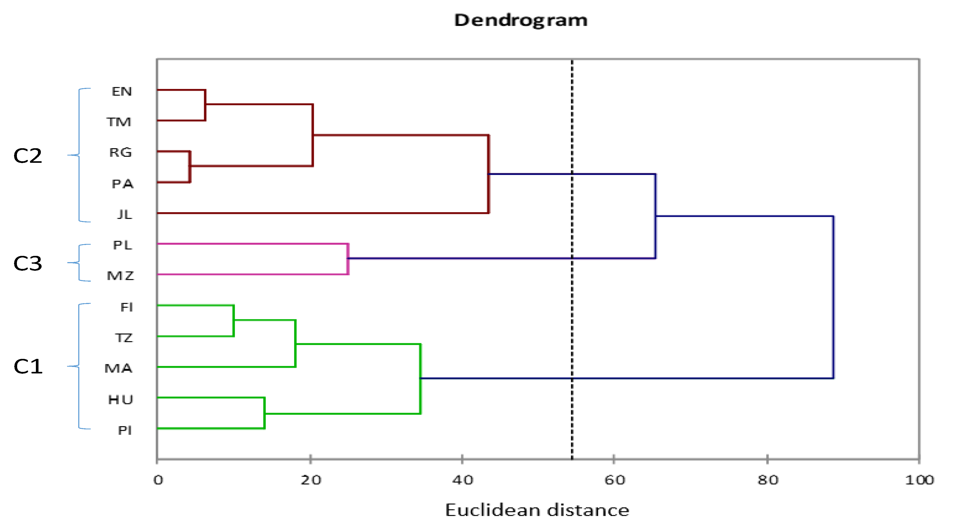
3.1. Clustering of Study Sites According to Their Physicochemical Properties
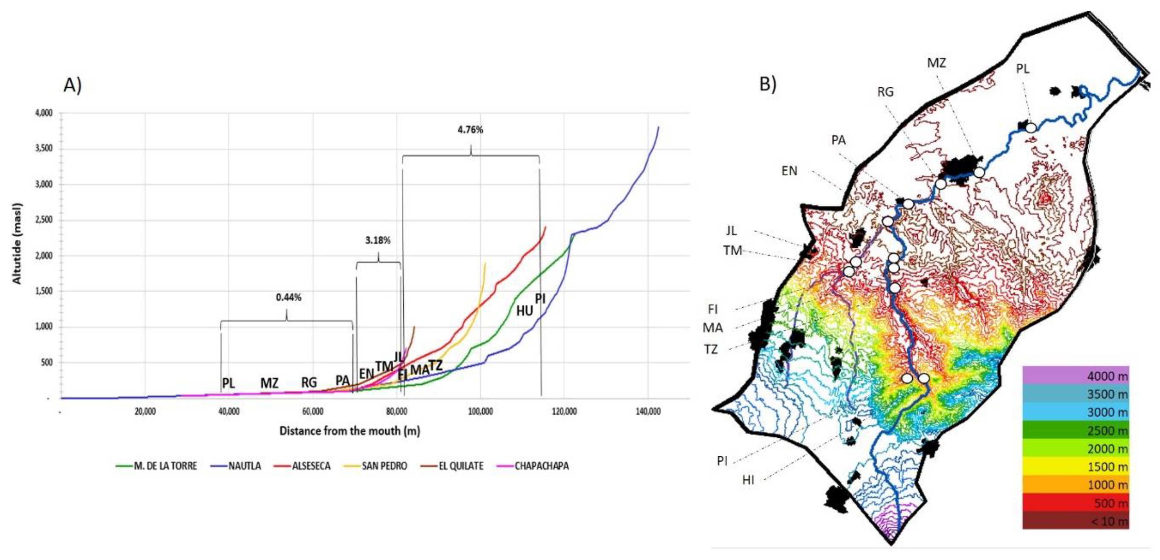
3.2. Longitudinal Profile of the River
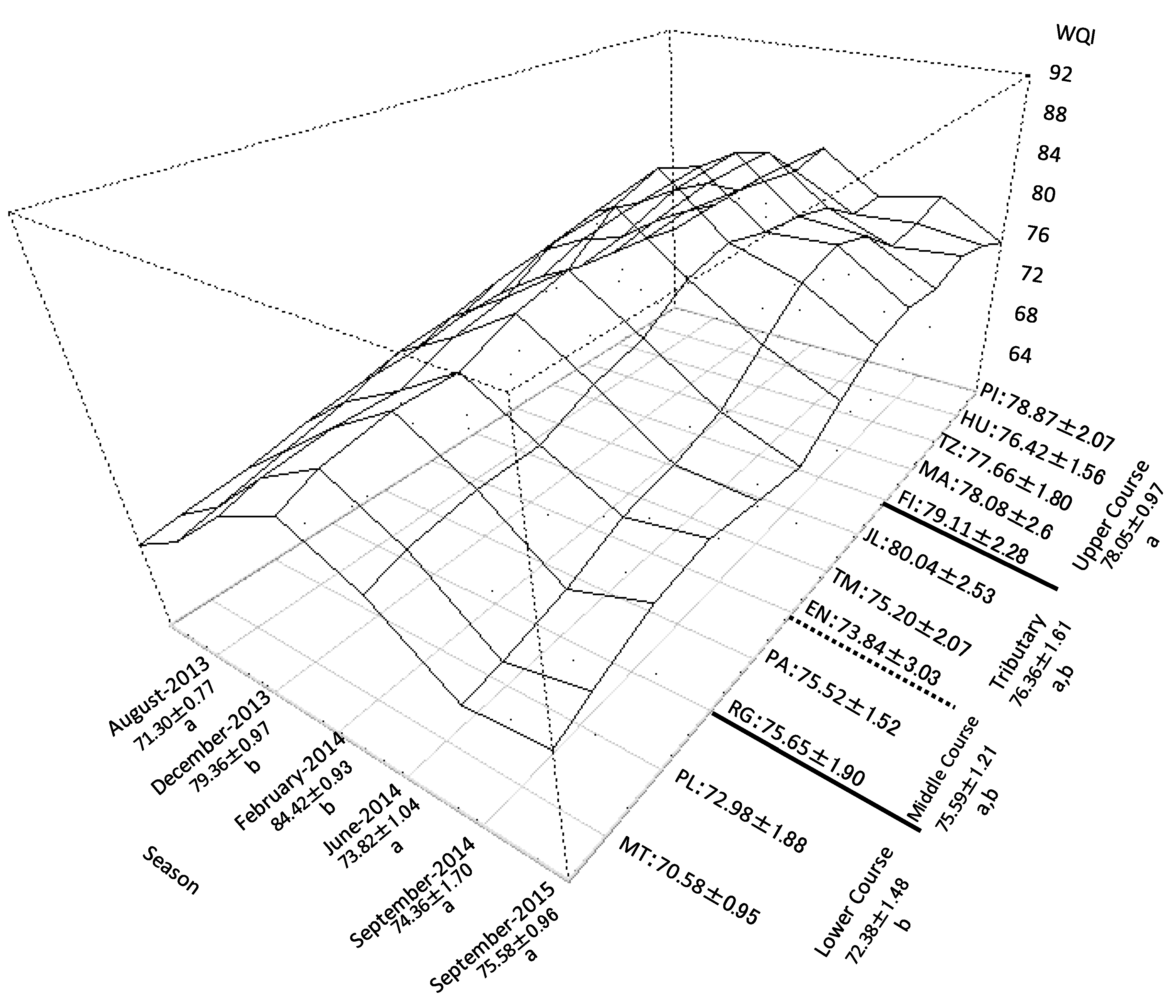
3.3. WQI
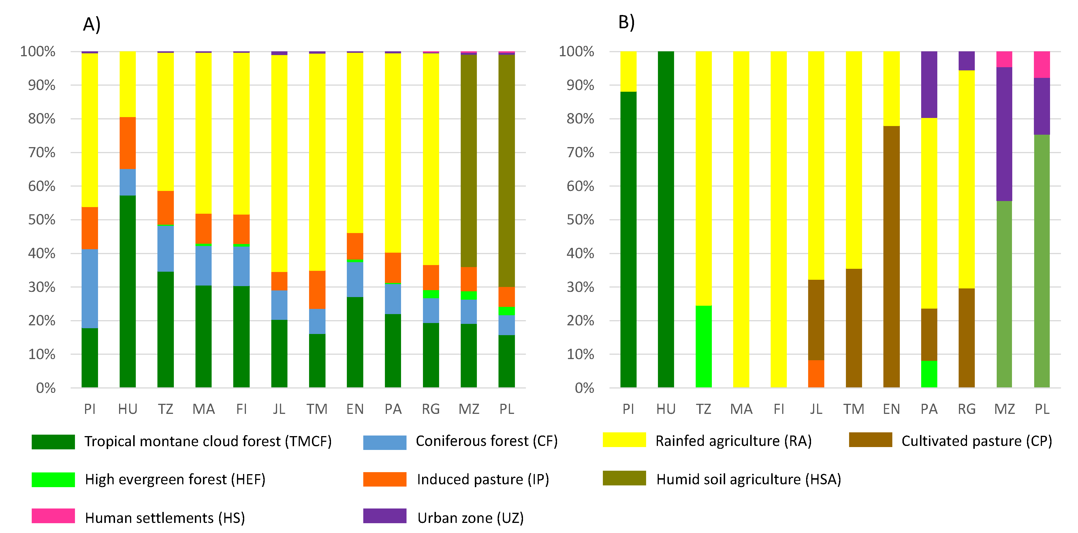
3.4. Land Uses
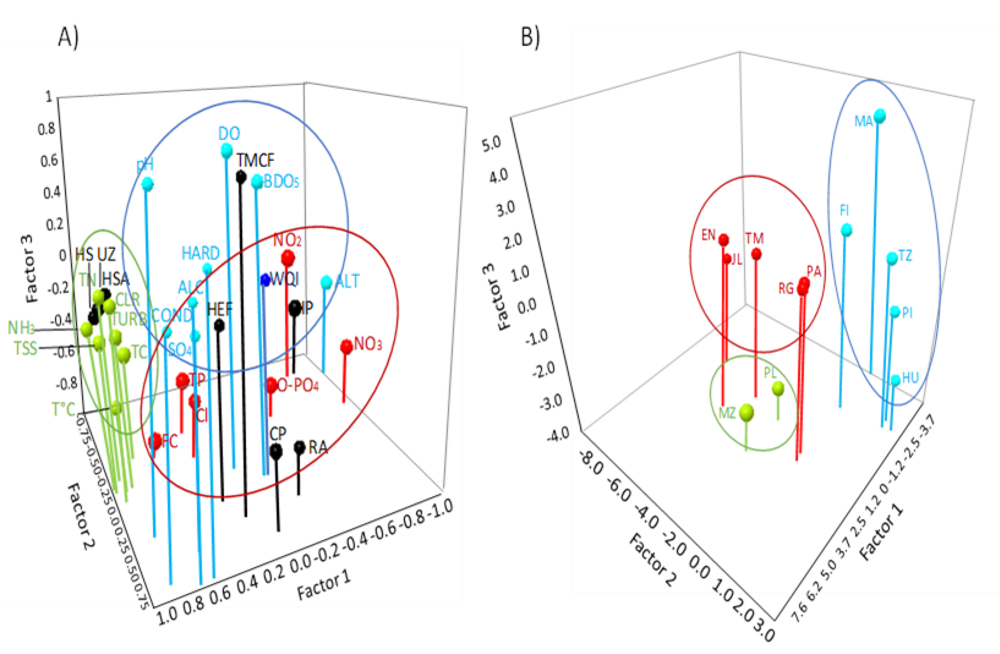
3.5. Multivariate Analysis
4. Discussion
5. Conclusions
Author Contributions
Funding
Acknowledgments
Conflicts of Interest
References
- Fan, M.; Shibata, H. Simulation of watershed hydrology and stream water quality under land use and climate change scenarios in Teshio River watershed, Northern Japan. Ecol. Indic. 2015, 50, 79–89. [Google Scholar] [CrossRef]
- Ding, J.; Jiang, Y.; Fu, L.; Liu, Q.; Peng, Q.; Kang, M. Impacts of land use on surface water quality in a subtropical River Basin: A case study of the Dongjiang River Basin, Southeastern China. Water 2015, 7, 4427–4445. [Google Scholar] [CrossRef]
- Rajib, M.A.; Ahiablame, L.; Paul, M. Modeling the effects of future land use change on water quality under multiple scenarios: A case study of low-input agriculture with hay/pasture production. Sustain. Water Qual. Ecol. 2016, 8, 50–66. [Google Scholar] [CrossRef]
- Kazi, T.G.; Arain, M.B.; Jamali, M.K.; Jalbani, N.; Afridi, H.I.; Sarfraz, R.A.; Baig, J.A.; Shah, A.Q. Assessment of water quality of polluted lake using multivariate statistical techniques: A case study. Ecotoxicol. Environ. Saf. 2009, 72, 301–309. [Google Scholar] [CrossRef] [PubMed]
- Peters, N.E.; Meybeck, M. Water quality degradation effects on freshwater availability: Impacts of human activities. Water Int. 2000, 25, 185–193. [Google Scholar] [CrossRef]
- Tong, S.T.Y.; Chen, W. Modeling the relationship between land use and surface water quality. J. Environ. Manag. 2002, 66, 377–393. [Google Scholar] [CrossRef]
- Xiao, R.; Wang, G.; Zhang, Q.; Zhang, Z. Multi-scale analysis of relationship between landscape pattern and urban river water quality in different seasons. Sci. Rep. 2016, 6, 25250. [Google Scholar] [CrossRef] [PubMed] [Green Version]
- Bennett, E.M.; Carpenter, S.R.; Caraco, N.F. Human impact on erodable phosphorus and eutrophication: A global perspective: Increasing accumulation of phosphorus in soil threatens rivers, lakes, and coastal oceans with eutrophication. AIBS Bull. 2001, 51, 227–234. [Google Scholar]
- Foley, J.A.; DeFries, R.; Asner, G.P.; Barford, C.; Bonan, G.; Carpenter, S.R.; Chapin, F.S.; Coe, M.T.; Daily, G.C.; Gibbs, H.K.; et al. Global consequences of land use. Science 2005, 309, 570–574. [Google Scholar] [CrossRef] [PubMed]
- Assessment, M.E. Ecosystem and Human Well-Being: Biodiversity Synthesis; World Resources Institute: Washington, DC, USA, 2005. [Google Scholar]
- Hansen, M.C.; Potapov, P.V.; Moore, R.; Hancher, M.; Turubanova, S.A.A.; Tyukavina, A.; Thau, D.; Stehman, S.V.; Goetz, S.J.; Loveland, T.R.; et al. High-resolution global maps of 21st-century forest cover change. Science 2013, 342, 850–853. [Google Scholar] [CrossRef] [PubMed]
- Keenan, R.J.; Reams, G.A.; Achard, F.; de Freitas, J.V.; Grainger, A.; Lindquist, E. Dynamics of global forest area: Results from the FAO Global Forest Resources Assessment 2015. For. Ecol. Manag. 2015, 352, 9–20. [Google Scholar] [CrossRef]
- Secretariat of Environment and Natural Resources (SEMARNAT). El Medio Ambiente en México 2013–2014; SEMARNAT: Mexico City, Mexico, 2014.
- Martínez, M.L.; Pérez-Maqueo, O.; Vázquez, G.; Castillo-Campos, G.; García-Franco, J.; Mehltreter, K.; Equihua, M.; Landgrave, R. Effects of land use change on biodiversity and ecosystem services in tropical montane cloud forests of Mexico. For. Ecol. Manag. 2009, 258, 1856–1863. [Google Scholar] [CrossRef]
- Thorne, R.S.J.; Williams, W.P. The response of benthic macroinvertebrate to pollution in developing countries: A multimetric system of bioassessment. Freshw. Biol. 1997, 37, 671–686. [Google Scholar] [CrossRef]
- Toledo-Aceves, T.; García-Franco, J.G.; Williams-Linera, G.; MacMillan, K.; Gallardo-Hernández, C. Significance of remnant cloud forest fragments as reservoirs of tree and epiphytic bromeliad diversity. Trop. Conserv. Sci. 2014, 7, 230–243. [Google Scholar] [CrossRef]
- Ponce-Reyes, R.; Reynoso-Rosales, V.-H.; Watson, J.E.M.; VanDerWal, J.; Fuller, R.A.; Pressey, R.L.; Possingham, H.P. Vulnerability of cloud forest reserves in Mexico to climate change. Nat. Clim. Chang. 2012, 2, 448–452. [Google Scholar] [CrossRef]
- Foster, P. The potential negative impacts of global climate change on tropical montane cloud forests. Earth-Sci. Rev. 2001, 55, 73–106. [Google Scholar] [CrossRef]
- Martınez-Morales, M.A. Landscape patterns influencing bird assemblages in a fragmented neotropical cloud forest. Biol. Conserv. 2005, 121, 117–126. [Google Scholar] [CrossRef]
- Ponce-Reyes, R.; Nicholson, E.; Baxter, P.W.J.; Fuller, R.A.; Possingham, H. Extinction risk in cloud forest fragments under climate change and habitat loss. Divers. Distrib. 2013, 19, 518–529. [Google Scholar] [CrossRef]
- Muñoz-Villers, L.E.; McDonnell, J.J. Land use change effects on runoff generation in a humid tropical montane cloud forest region. Hydrol. Earth Syst. Sci. 2013, 17, 3543–3560. [Google Scholar] [CrossRef] [Green Version]
- McDowell, W.H.; Asbury, C.E. Export of carbon, nitrogen, and major ions from three tropical montane watersheds. Limnol. Oceanogr. 1994, 39, 111–125. [Google Scholar] [CrossRef] [Green Version]
- Turner, W.R.; Brandon, K.; Brooks, T.M.; Costanza, R.; da Fonseca, G.A.B.; Portela, R. Global Conservation of Biodiversity and Ecosystem Services. BioScience 2007, 57, 868–873. [Google Scholar] [CrossRef] [Green Version]
- Quétier, F.; Lavorel, S.; Thuiller, W.; Davies, I. Plant-trait-based modeling assessment of ecosystem-service sensitivity to land-use change. Ecol. Appl. 2007, 17, 2377–2386. [Google Scholar] [CrossRef] [PubMed]
- Martínez, M.L.; Manson, R.H.; Balvanera, P.; Dirzo, R.; Soberón, J.; García-Barrios, L.; Martínez-Ramos, M.; Moreno-Casasola, P.; Rosenzweig, L.; Sarukhán, J. The evolution of ecology in Mexico: Facing challenges and preparing for the future. Front. Ecol. Environ. 2006, 4, 259–267. [Google Scholar] [CrossRef]
- Tu, J. Spatial and temporal relationships between water quality and land use in northern Georgia, USA. J. Integr. Environ. Sci. 2011, 8, 151–170. [Google Scholar] [CrossRef] [Green Version]
- Hutchinson, K.J.; Christiansen, D.E. Use of the Soil and Water Assessment Tool (SWAT) for Simulating Hydrology and Water Quality in the Cedar River Basin, Iowa, 2000–10; Scientific Investigations Report 2013–5002; U.S. Geological Survey (USGS): Reston, VA, USA, 2013.
- Schönhart, M.; Trautvetter, H.; Parajka, J.; Blaschke, A.P.; Hepp, G.; Kirchner, M.; Mitter, H.; Schmid, E.; Strenn, B.; Zessner, M. Modelled impacts of policies and climate change on land use and water quality in Austria. Land Use Policy 2018, 76, 500–514. [Google Scholar] [CrossRef]
- Kang, J.-H.; Lee, S.W.; Cho, K.H.; Ki, S.J.; Cha, S.M.; Kim, J.H. Linking land-use type and stream water quality using spatial data of fecal indicator bacteria and heavy metals in the Yeongsan river basin. Water Res. 2010, 44, 4143–4157. [Google Scholar] [CrossRef] [PubMed]
- Bengraïne, K.; Marhaba, T.F. Using principal component analysis to monitor spatial and temporal changes in water quality. J. Hazard. Mater. 2003, 100, 179–195. [Google Scholar] [CrossRef]
- Reghunath, R.; Murthy, T.R.S.; Raghavan, B.R. The utility of multivariate statistical techniques in hydrogeochemical studies: An example from Karnataka, India. Water Res. 2002, 36, 2437–2442. [Google Scholar] [CrossRef]
- Simeonov, V.; Stratis, J.A.; Samara, C.; Zachariadis, G.; Voutsa, D.; Anthemidis, A.; Sofoniou, M.; Kouimtzis, T. Assessment of the surface water quality in Northern Greece. Water Res. 2003, 37, 4119–4124. [Google Scholar] [CrossRef]
- Brodnjak-Vončina, D.; Dobčnik, D.; Novič, M.; Zupan, J. Chemometrics characterisation of the quality of river water. Anal. Chim. Acta 2002, 462, 87–100. [Google Scholar] [CrossRef]
- Singh, K.P.; Malik, A.; Sinha, S. Water quality assessment and apportionment of pollution sources of Gomti river (India) using multivariate statistical techniques—A case study. Anal. Chim. Acta 2005, 538, 355–374. [Google Scholar] [CrossRef]
- Danielsson, Å.; Cato, I.; Carman, R.; Rahm, L. Spatial clustering of metals in the sediments of the Skagerrak/Kattegat. Appl. Geochem. 1999, 14, 689–706. [Google Scholar] [CrossRef]
- Zhou, F.; Liu, Y.; Guo, H. Application of multivariate statistical methods to water quality assessment of the watercourses in Northwestern New Territories, Hong Kong. Environ. Monit. Assess. 2007, 132, 1–13. [Google Scholar] [CrossRef] [PubMed]
- Wenning, R.J.; Erickson, G.A. Interpretation and analysis of complex environmental data using chemometric methods. TrAC Trends Anal. Chem. 1994, 13, 446–457. [Google Scholar] [CrossRef]
- Arslan, O. A GIS-based spatial-Multivariate statistical analysis of water quality data in the Porsuk River, Turkey. Water Qual. Res. J. 2009, 44, 279–293. [Google Scholar] [CrossRef]
- Instituto Nacional de Estadística Geografía e Informática (INEGI). Carta Geológica-Minera Altotonga E14-B16, 1:50,000; INEGI: Aguascalientes, Mexico, 2010.
- American Public Health Association (APHA). Standard Methods for the Examination of Water and Wastewater, 21st ed.; APHA: Washington, DC, USA, 2005; p. 1220.
- Dinius, S.H. Design of an Index of Water Quality. J. Am. Water Resour. Assoc. 1987, 23, 833–843. [Google Scholar] [CrossRef]
- SIATL|Simulador de Flujos de Agua de Cuencas Hidrográficas. Available online: http://antares.inegi.org.mx/analisis/red_hidro/siatl/# (accessed on 16 October 2018).
- Boyd, C.E. Water Quality: An Introduction; Springer: Berlin, Germany, 2015; ISBN 9783319174464. [Google Scholar]
- Tromboni, F.; Dodds, W.K. Relationships between land use and stream nutrient concentrations in a highly urbanized tropical region of Brazil: Thresholds and riparian zones. Environ. Manag. 2017, 60, 30–40. [Google Scholar] [CrossRef] [PubMed]
- Carpenter, S.R.; Al, E. Nonpoint pollution of surface waters with phosphorus and nitrogen. Ecol. Appl. 1998, 8, 559–568. [Google Scholar] [CrossRef]
- Buck, O.; Niyogi, D.K.; Townsend, C.R. Scale-dependence of land use effects on water quality of streams in agricultural catchments. Environ. Pollut. 2004, 130, 287–299. [Google Scholar] [CrossRef] [PubMed]
- Nilsson, C.; Renöfält, B.M. Linking flow regime and water quality in rivers: A challenge to adaptive catchment management. Ecol. Soc. 2008, 13, 18. [Google Scholar] [CrossRef]
- Solaimani, K.; Arekhi, M.; Tamartash, R.; Miryaghobzadeh, M. Land use/cover change detection based on remote sensing data (A case study; Neka Basin). Agric. Biol. J. N. Am. 2010, 1, 1148–1157. [Google Scholar] [CrossRef]
- Permatasari, P.A.; Setiawan, Y.; Khairiah, R.N.; Effendi, H. The effect of land use change on water quality: A case study in Ciliwung Watershed. In IOP Conference Series: Earth and Environmental Science; IOP Publishing: Bristol, UK, 2017. [Google Scholar] [CrossRef]
- Rodríguez-Romero, A.J.; Rico-Sánchez, A.E.; Catalá, M.; Sedeño-Díaz, J.E.; López-López, E. Mitochondrial activity in fern spores of Cyathea costaricensis as an indicator of the impact of land use and water quality in rivers running through cloud forests. Chemosphere 2017, 189, 435–444. [Google Scholar] [CrossRef] [PubMed]
- González, S.O.; Almeida, C.A.; Calderón, M.; Mallea, M.A.; González, P. Assessment of the water self-purification capacity on a river affected by organic pollution: Application of chemometrics in spatial and temporal variations. Environ. Sci. Pollut. Res. 2014, 21, 10583–10593. [Google Scholar] [CrossRef] [PubMed]
- Costa, M.H.; Botta, A.; Cardille, J.A. Effects of large-scale changes in land cover on the discharge of the Tocantins River, Southeastern Amazonia. J. Hydrol. 2003, 283, 206–217. [Google Scholar] [CrossRef]
- Sliva, L.; Williams, D.D. Buffer zone versus whole catchment approaches to studying land use impact on river water quality. Water Res. 2001, 35, 3462–3472. [Google Scholar] [CrossRef]
- Li, S.; Gu, S.; Tan, X.; Zhang, Q. Water quality in the Upper Han River basin, China: The impacts of land use/land cover in riparian buffer zone. J. Hazard. Mater. 2009, 165, 317–324. [Google Scholar] [CrossRef] [PubMed]
- Gove, N.E.; Edwards, R.T.; Conquest, L.L. Effects of scale on land use and water quality relationships: A longitudinal basin-wide perspective. J. Am. Water Resour. Assoc. 2001, 37, 1721–1734. [Google Scholar] [CrossRef]
- Wu, Y.; Liu, S.; Sohl, T.L.; Young, C.J. Projecting the land cover change and its environmental impacts in the Cedar River Basin in the Midwestern United States. Environ. Res. Lett. 2013, 8, 024025. [Google Scholar] [CrossRef] [Green Version]
- Rajib, A.; Merwade, V. Hydrologic response to future land use change in the Upper Mississippi River Basin by the end of 21st century. Hydrol. Process. 2017, 31, 3645–3661. [Google Scholar] [CrossRef]
- Sleeter, B.M.; Sohl, T.L.; Bouchard, M.A.; Reker, R.R.; Soulard, C.E.; Acevedo, W.; Griffith, G.E.; Sleeter, R.R.; Auch, R.F.; Sayler, K.L.; et al. Scenarios of land use and land cover change in the conterminous United States: Utilizing the special report on emission scenarios at ecoregional scales. Glob. Environ. Chang. 2012, 22, 896–914. [Google Scholar] [CrossRef]


| Parameter | F1 (35.56%) | F2 (20.91%) | F3 (13.03%) |
|---|---|---|---|
| DO | −0.0871 | −0.0171 | 0.8850 |
| pH | 0.3879 | 0.3074 | 0.6906 |
| COND | 0.0979 | 0.7551 | −0.3434 |
| TURB | 0.8437 | −0.1793 | 0.1031 |
| T (°C) | 0.7824 | 0.1094 | −0.4135 |
| NO3 | −0.7053 | −0.5861 | −0.0335 |
| NO2 | −0.1607 | −0.6586 | 0.5103 |
| NH3 | 0.9559 | 0.1313 | 0.0420 |
| TN | 0.8492 | 0.1585 | 0.1872 |
| O–PO4 | −0.0362 | −0.6673 | −0.0824 |
| TP | 0.5200 | −0.5171 | −0.0259 |
| SO4 | −0.1264 | 0.6642 | −0.3709 |
| BDO5 | −0.2876 | −0.0906 | 0.7283 |
| TC | 0.8242 | −0.2818 | 0.0543 |
| FC | 0.7499 | −0.5891 | −0.2426 |
| TSS | 0.9432 | −0.1323 | 0.0726 |
| HARD | −0.3486 | 0.8449 | −0.0211 |
| ALC | −0.1793 | 0.8110 | −0.2087 |
| Cl− | 0.3173 | −0.2528 | −0.2921 |
| ALT | −0.8523 | −0.1603 | 0.1463 |
| CLR | 0.8230 | −0.0156 | 0.1958 |
| TMCF | −0.4623 | 0.4379 | 0.6355 |
| HEF | −0.1492 | 0.2514 | −0.1479 |
| IP | −0.1868 | −0.7041 | 0.2858 |
| CP | −0.0485 | −0.7128 | −0.4024 |
| RA | −0.4603 | −0.4009 | −0.6416 |
| HSA | 0.7789 | 0.2416 | 0.1623 |
| UZ | 0.8628 | 0.2615 | 0.0455 |
| HS | 0.8325 | 0.2567 | 0.0858 |
| WQI | −0.5758 | 0.2582 | 0.0610 |
| Site | NO3 (mg/L) | NO2 (mg/L) | NH3 (mg/L) | TN (mg/L) | O–PO4 (mg/L) | TP (mg/L) | WQI | Predominant Land Use |
|---|---|---|---|---|---|---|---|---|
| PI | 1.17 (±1.007) | 0.007 (±0.004) | 0.19 (±0.09) | 7.94 (±3.43) | 0.47 (±0.13) | 0.76 (±0.4) | 76.42 ± 1.60 | TMCF (100%) |
| HU | 1.02 (±0.1) | 0.007 (±0.002) | 0.18 (±0.04) | 6.63 (±2.18) | 0.31 (±0.31) | 0.59 (±0.1) | 78.87 ± 2.11 | TMCF (92%) |
| TZ | 0.97 (±0.09) | 0.007 (±0.001) | 0.21 (±0.02) | 8.16 (±2.17) | 0.34 (±0.07) | 0.65 (±0.12) | 76.66 ± 1.97 | RA (77.6%) |
| MA | 1.34 (±0.13) | 0.006 (±0.001) | 0.19 (±0.01) | 7.45 (±2) | 0.48 (±0.08) | 0.72 (±0.07) | 78.08 ± 2.48 | RA (96%) |
| FI | 0.96 (±0.09) | 0.005 (±0.001) | 0.25 (±0.06) | 8.56 (±1.56) | 0.51 (±0.1) | 0.89 (±0.13) | 79.11 ± 2.50 | RA (79.11%) |
| JL | 1.46 (±0.22) | 0.013 (±0.003) | 0.21 (±0.03) | 7.65 (±2.02) | 0.56 (±0.07) | 0.8 (±0.12) | 80.04 ± 2.77 | RA (67%) |
| TM | 1.27 (±0.3) | 0.011 (±0.004) | 0.26 (±0.1) | 8.05 (±3.42) | 0.53 (±0.17) | 0.93 (±0.4) | 75.20 ± 2.27 | RA (59%) |
| EN | 1.21 (±0.25) | 0.008 (±0.002) | 0.3 (±0.12) | 9.31 (±1.95) | 0.66 (±0.05) | 1.23 (±0.3) | 73.84 ± 3.32 | CP (79%) |
| PA | 1.07 (±0.15) | 0.008 (±0.002) | 0.27 (±0.08) | 9.34 (±2.43) | 0.45 (±0.07) | 0.8 (±0.15) | 75.52 ± 1.62 | RA, HS (59%, 14%) |
| RG | 1.03 (±0.16) | 0.007 (±0.002) | 0.27 (±0.05) | 9.89 (±2.8) | 0.4 (±0.1) | 0.74 (±0.08) | 75.65 ± 2.08 | RA (67%) |
| MZ | 0.53 (±0.39) | 0.005 (±0.005) | 0.48 (±0.45) | 10.15 (±9.69) | 0.25 (±0.03) | 0.79 (±0.20) | 70.58 ± 1.35 | HSA, HS, UZ (62%, 32%, 6%) |
| PL | 1.12 (±0.1) | 0.008 (±0.002) | 0.35 (±0.14) | 9.96 (±2.9) | 0.64 (±0.16) | 1.08 (±0.33) | 72.98 ± 2.06 | HSA, HS, UZ (76%, 23%, 1%) |
© 2018 by the authors. Licensee MDPI, Basel, Switzerland. This article is an open access article distributed under the terms and conditions of the Creative Commons Attribution (CC BY) license (http://creativecommons.org/licenses/by/4.0/).
Share and Cite
Rodríguez-Romero, A.J.; Rico-Sánchez, A.E.; Mendoza-Martínez, E.; Gómez-Ruiz, A.; Sedeño-Díaz, J.E.; López-López, E. Impact of Changes of Land Use on Water Quality, from Tropical Forest to Anthropogenic Occupation: A Multivariate Approach. Water 2018, 10, 1518. https://doi.org/10.3390/w10111518
Rodríguez-Romero AJ, Rico-Sánchez AE, Mendoza-Martínez E, Gómez-Ruiz A, Sedeño-Díaz JE, López-López E. Impact of Changes of Land Use on Water Quality, from Tropical Forest to Anthropogenic Occupation: A Multivariate Approach. Water. 2018; 10(11):1518. https://doi.org/10.3390/w10111518
Chicago/Turabian StyleRodríguez-Romero, Alexis Joseph, Axel Eduardo Rico-Sánchez, Erick Mendoza-Martínez, Andrea Gómez-Ruiz, Jacinto Elías Sedeño-Díaz, and Eugenia López-López. 2018. "Impact of Changes of Land Use on Water Quality, from Tropical Forest to Anthropogenic Occupation: A Multivariate Approach" Water 10, no. 11: 1518. https://doi.org/10.3390/w10111518