Drought Analysis in the Yellow River Basin Based on a Short-Scalar Palmer Drought Severity Index

1
School of Hydrology and Water Resources, Nanjing University of Information Science & Technology, Nanjing 210044, China
2
State Key Laboratory of Hydrology-Water Resources and Hydraulic Engineering, Hohai University, Nanjing 210098, China
3
Department of Biological and Agricultural Engineering, Texas A&M University, College Station, TX 77843-2117, USA
*
Author to whom correspondence should be addressed.
Water 2018, 10(11), 1526; https://doi.org/10.3390/w10111526
Submission received: 28 September 2018
/
Revised: 16 October 2018
/
Accepted: 23 October 2018
/
Published: 26 October 2018
(This article belongs to the Section Hydrology)
Abstract
:Focusing on the shortages of moisture estimation and time scale in the self-calibrating Palmer drought severity index (scPDSI), this study proposed a new Palmer variant by introducing the Variable Infiltration Capacity (VIC) model in hydrologic accounting module, and modifying the standardization process to make the index capable for monitoring droughts at short time scales. The performance of the newly generated index was evaluated over the Yellow River Basin (YRB) during 1961–2012. For time scale verification, the standardized precipitation index (SPI), and standardized precipitation evapotranspiration index (SPEI) at a 3-month time scale were employed. Results show that the new Palmer variant is highly correlated with SPI and SPEI, combined with a more stable behavior in drought frequency than original scPDSI. For drought trend detection, this new index is more inclined to reflect comprehensive moisture conditions and reveals a different spatial pattern from SPI and SPEI in winter. Besides, two remote sensing products of soil moisture and vegetation were also employed for comparison. Given their general consistent behaviors in monitoring the spatiotemporal evolution of the 2000 drought, it is suggested that the new Palmer variant is a good indicator for monitoring soil moisture variation and the dynamics of vegetation growth.
1. Introduction
Drought is one of the costliest natural hazards which have caused tremendous disruptions to past and modern societies [1]. Drought affects both surface and groundwater resources, which potentially threaten crop production, water quality, waterborne transportation, power generation, economy and social activities [2]. Due to the enhanced pressure from global warming and socioeconomic developments, problems of water shortage have been further aggravated, and drought risks are expected to increase [3,4,5]. To prevent and mitigate the potential damage from drought, it is crucial to improve drought monitoring, management and forecasting techniques [2,6]. The main difficulty of this work lies in how to pinpoint the onset and termination time of a drought accurately, as well as to quantify its characteristics like duration, severity, and affecting area [7]. Drought indices are one of the effective tools which allow timely identification and characterization of emerging drought conditions [8].
From the perspective of hydrological variables, drought indices generally experienced a development process from incorporating one single variable to bivariate or multiple variables [9]. For example, in earlier researches, precipitation was mostly employed to indicate the climatic dry conditions, such as the precipitation percentile and deciles [10]. The Palmer drought severity index (PDSI) [11] is one exception during the early period. In its moisture estimation section, the concept of soil water balance model was firstly introduced, which could be recognized as the pioneer of multivariate-based drought indices. However, this scheme was not widely extended due to its coarse delineation of the hydrological process and unsatisfying performance in frozen and snow areas [12,13]. With increased knowledge of drought, the non-negligible role of other hydrological variables (e.g., evapotranspiration and soil moisture) has been highlighted in recent years. A variety of new indices involving different factors were proposed. For example, some indices incorporated evapotranspiration in their algorithms to reflect the effects of global warming on drought, such as the reconnaissance drought index (RDI) [14], standardized precipitation evapotranspiration index (SPEI) [15], and evaporative demand drought index (EDDI) [16]. The composite drought indices such as the aggregate drought index (ADI) [17] and joint drought deficit index (JDI) [18] represent another category of drought indices which integrated multiple hydro-meteorological variables with different statistical models [19]. Moreover, enlightened by PDSI, the introduction of more mature hydrological models within the index also became popular [20,21]. Generally, a comprehensive consideration of hydrological components is the main development direction of drought indices.
Apart from moisture status estimation, the ability to indicate droughts at different time scales is another important feature of drought indices. The earliest proposal of this concept could be traced back to the standardized precipitation index (SPI) [22], in which an explicit definition of time scale was presented according to the time period of water deficits are accumulated. This concept was further applied in other standardized drought indices, such as SPEI and standardized runoff index (SRI) [23]. The PDSI represents another drought index category without a specific illustration of time scale in their algorithms [24]. This shortage largely limits its application, since drought in nature is a multi-scalar phenomenon, and a versatile drought index ideally should be capable of reflecting drought conditions at different time scales [25]. A recent literature [26] solved this problem which extended the time scale of the self-calibrating PDSI (scPDSI; a revised version of PDSI which improves the spatiotemporal comparability of the index [27]) into a wide range.
Focusing on above mentioned two aspects, this study aimed at constructing a new variant of the palmer index by (i) replacing the original moisture estimation module with more mature hydrological model, and (ii) modifying the standardization procedure of scPDSI and analyzing its capability in monitoring drought conditions at short time scales (including seasonal drought trend, vegetation condition and soil moisture anomalies). This paper is organized as follows. Section 2 describes the study area and datasets used in this study. An introduction of hydrological model and modifications on the scPDSI is provided in Section 3. Section 4 discusses the performances of the new drought index in term of time scale, drought trend and drought events monitoring. Conclusions are given in Section 5.
2. Study Area and Data
2.1. Study Area
The Yellow River Basin (YRB) is located between 32° N–42° N and 96° E–119° E (Figure 1), controlling a drainage area of 795,000 km2. From northwest to southeast, the elevation presents a gradually decreased pattern and ranges between 1 and 6199 m above the sea level. The Tibet Plateau, Loess Plateau and Huang-Huai-Hai Plain are three primary geomorphic types of this basin [28]. Climatically, the mean annual temperature varies between 4 and 14 °C. Precipitation is unevenly distributed over YRB which divides the whole basin into four climate zones from northwest to southeast, i.e., arid, semi-arid, semi-humid and humid zones. In addition, precipitation and temperature have significant seasonality, where summer is generally rainy and hot while winter is cold and dry.
2.2. Data
The forcing data for running the hydrological model includes hydro-meteorological observations and geographic information. Daily records of precipitation, mean temperature, maximum and minimum temperatures, and wind speed from 101 national meteorological stations in and around YRB (Figure 1) were downloaded from the China Meteorological Data Service Centre (http://data.cma.cn/). Historical streamflow data of 10 hydrological stations [i.e., Tangnaihai (TNH), Lanzhou (LZ), Toudaoguai (TDG), Wubao (WB), Longmen (LM), Hejin (HJ), Xianyang (XY), Huaxian (HX), Sanmenxia (SMX), and Huayuankou (HYK)] situated at the trunk stream and main tributaries were collected from “China Year Books of Hydrology”. Detailed information on the coordinates, elevation, drainage area and areal average precipitation of these hydrological stations is listed in Table 1. All hydro-meteorological observations have complete daily records from 1961 to 2012. The geographic images were gathered as follows: the 3 arc-second (about 90 m) digital elevation image was retrieved from the shuttle radar topography mission digital elevation model (http://srtm.csi.cgiar.org/); the land cover map was provided by the University of Maryland’s 1 km Global Land Cover Production [29]; and soil data with a 30 arc-second spatial resolution was from the 5-min Food and Agriculture Organization dataset [12].
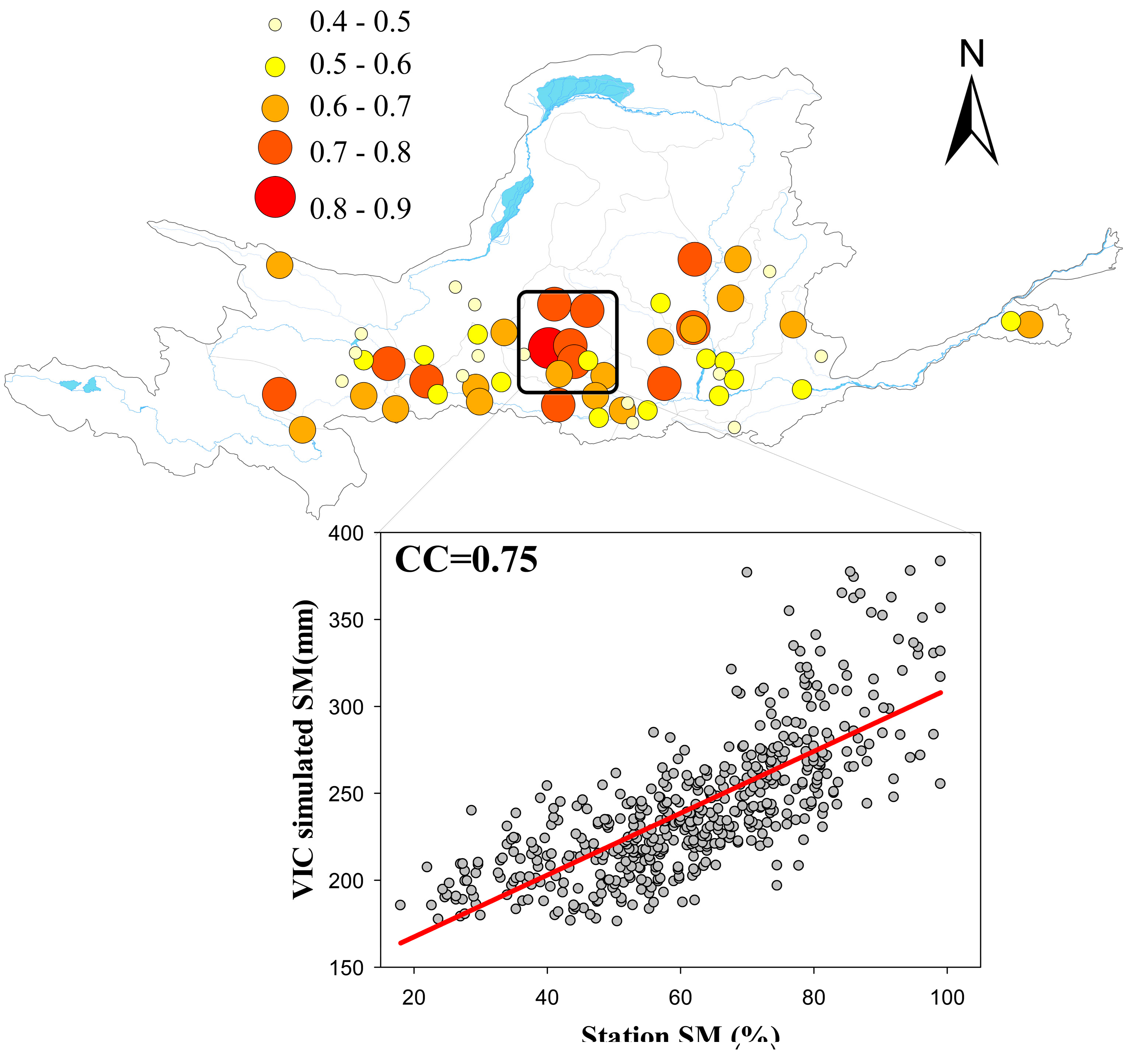
To verify the accuracy of model simulated soil moisture, the measured soil moisture dataset of the China Agrometeorological Stations [30] were employed. This dataset provides 10-day relative soil moisture records at five (i.e., 10-cm, 20-cm, 50-cm, 70-cm, and 100-cm) soil depths. In this study, the data of 50-cm soil layer with relatively complete records (available from September 1991 to December 2008). After quality checkup, 57 sites with relatively complete observations were selected in this study (see Figure 1 for their spatial distributions).
The remote sensing soil moisture data from the Climate Change Initiative (CCI) program, released by the European Space Agency (ESA), was also collected. This product (named ESACCI-SM) combines various active and passive microwave soil moisture products, and is regularly updated. Compared to other remote sensing products, the ESACCI-SM has a rather long period of coverage, making it more suitable to assess the long-term variability and change of surface soil moisture [31]. The soil moisture dataset was available daily from 1978–2015 with a spatial resolution of 0.25°, and in this study it was employed to reflect soil moisture-based dry conditions.
In addition, to investigate the response of improved drought index to vegetation activity, the Global Inventory Modeling and Mapping Studies-Normalized Difference Vegetation Index (GIMMS-NDVI) dataset was introduced. This dataset was available semimonthly from 1982 to 2015 with a resolution of 8 km. To facilitate comparison, values of NDVI were processed into the monthly average values, and spatially they were resampled into 0.25° resolution.
3. Methods
3.1. VIC Model Simulation
The physically based macroscale Variable Infiltration Capacity (VIC) model [32] was used for hydrological simulation over YRB. The model considers both water and energy balances within each grid cell, and can represent subgrid variability in terrain characteristics, land surface vegetation classes, and soil features (including soil texture, depths, and moisture storage capacity). In this study, the latest version of VIC which partitions the subsurface into three layers (VIC-3L), was employed. A detailed description of VIC-3L is referred to Liang et al. [33].
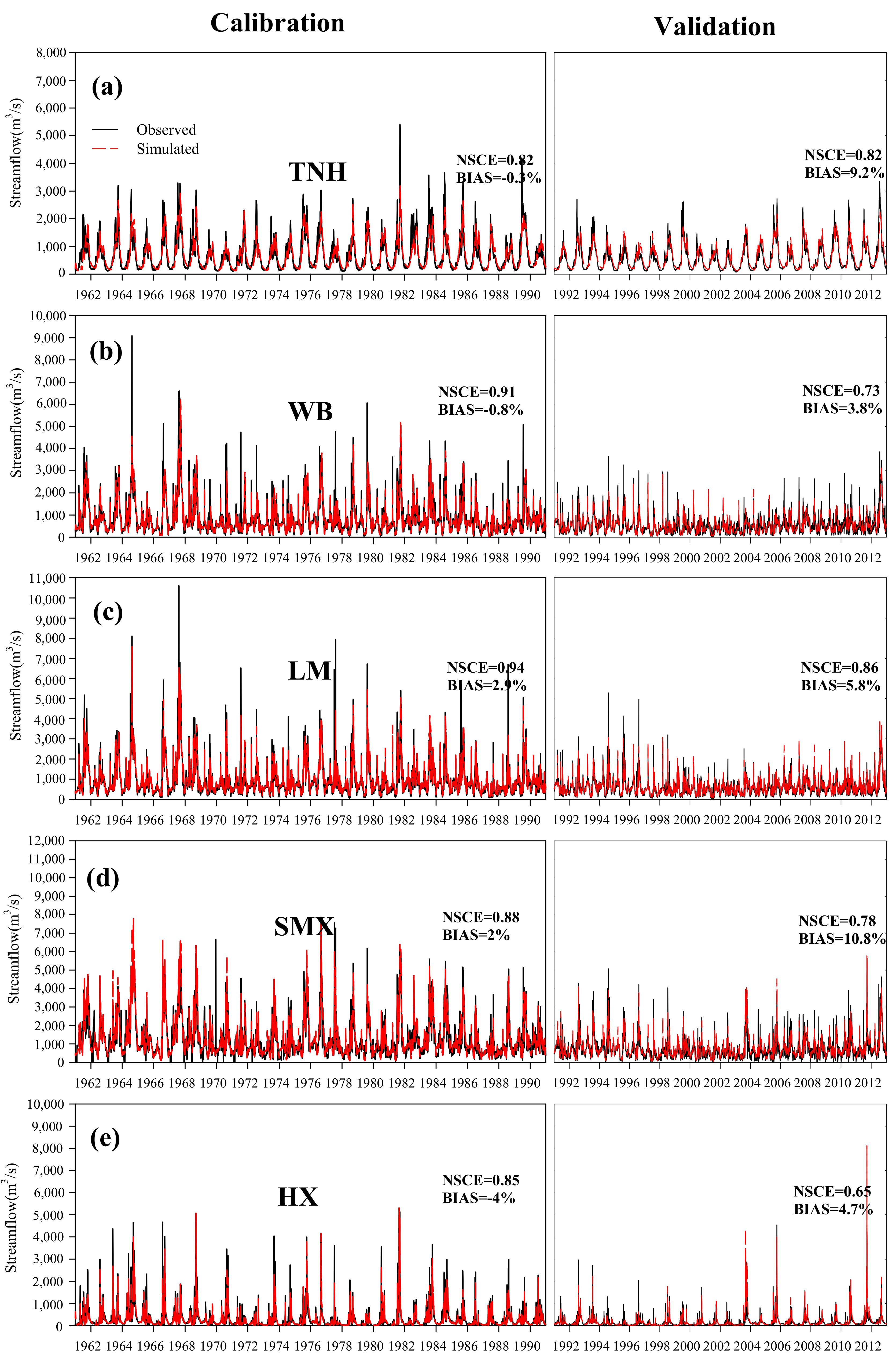
For model implementation, VIC was run at a daily time step and 0.25° spatial resolution over the whole YRB (the basin was divided into 1500 grids). All site-based meteorological forcings were interpolated into each grid through the inverse distance weighted (IDW) method. Likewise, geographic data including the elevation, soil, and vegetation images were resampled into the 0.25° spatial resolution. Daily streamflow records of 10 hydrological stations were used to calibrate the model during 1961–1990, while for the validation periods (1991–2012), both streamflow and soil moisture data from observation sites (see Figure 1 for their locations) were employed. The consistency degree between simulated hydrological variables and observed ones was measured through three appraisement coefficients, i.e., the Nash-Sutcliffe coefficient of efficiency (NSCE), BIAS and correlation coefficient (CC).
3.2. Modified scPDSI
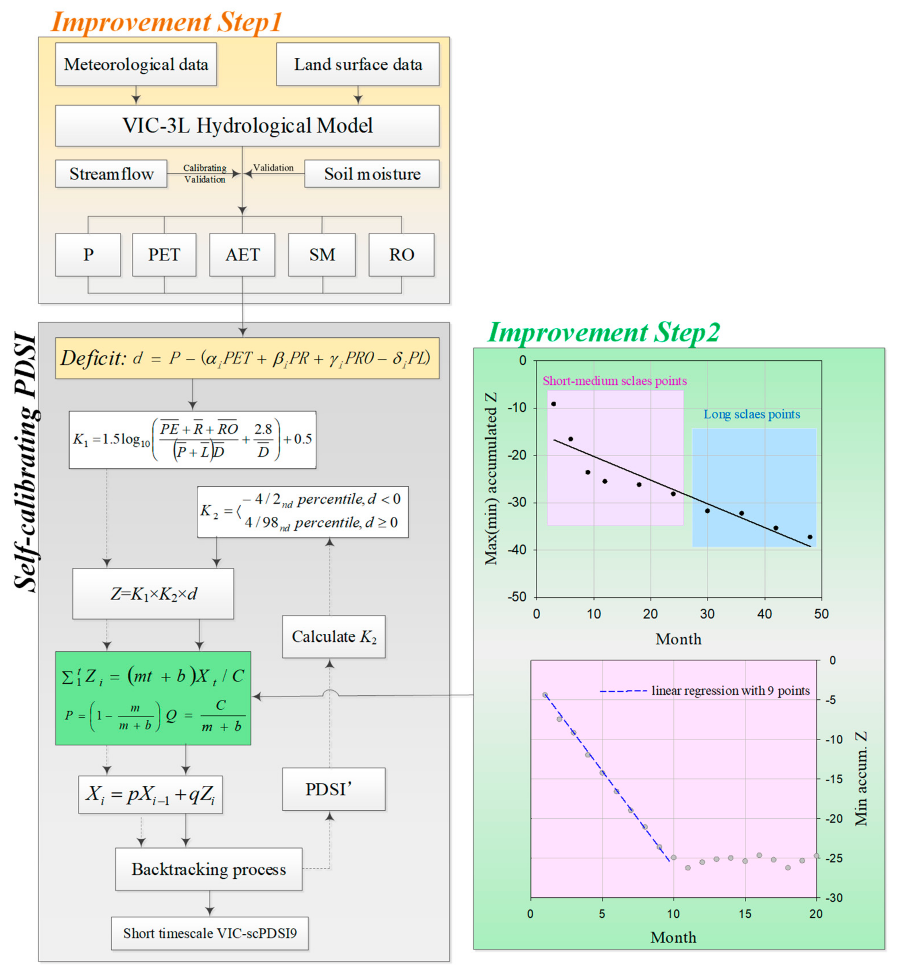
The scPDSI is an advanced version of PDSI aimed at improving the spatiotemporal comparability of the index. Compared to the original algorithm [11], Wells et al. [27] introduced a new climate characteristic K2 which could correct the high frequency of extreme events and realize automatic calibration of the index behaviors at any locations (Figure 2). Focusing on the hydrologic accounting module (improvement 1) and standardization process (improvement 2), further modifications on scPDSI were conducted in following sections to address the shortcomings of moisture estimation and time scale. Implementation of the method was based on the source code (compiling in Visual C) of scPDSI, which was downloaded from the National Agricultural Decision Support System (NADSS, available online at http://nadss.unl.edu/).
3.2.1. Coupling VIC Model for Hydrologic Accounting
The hydrologic accounting of scPDSI involves eight variables, including evapotranspiration (ET), recharge (R), runoff (RO), loss (L), potential evapotranspiration (PET), potential recharge (PR), potential runoff (PRO), and potential loss (PL). In Palmer’s scheme [11], the climatically appropriate for existing conditions (CAFEC) precipitation () was introduced to represent the amount of precipitation needed to maintain a normal soil moisture level. The moisture deficit d for a specific month is defined as the difference between actual precipitation (P) and :
where Pi and represent the water supply and demand for the ith (i = 1, 2, …, 12) month in a calendar year. α, β, γ, and δ are weighting coefficients defined in the following manner:
where the bar over a variable denotes the average value of ith month. In the original algorithm, these eight variables are estimated from a simplified two-stage bucket model, where the available water holding capacity (AWC) of the soil plays an important role in determining the moisture movement (see Palmer [11] for detail). In this study, the hydrologic accounting was conducted on basis of VIC simulations instead. As shown in Figure 2, P, ET, RO, and PET can be directly extracted from the outputs of the hydrological model. It should be noted that the PET estimated by VIC is based on the Penman-Monteith equation [34], in which the air temperature, wind speed, atmospheric and vapor pressure are required as the inputting variables. Other five variables can be estimated through following equations [11,20]:
where AWC is the same as defined by Palmer [11], and is taken as the difference between filed capacity and wilting moisture of the whole soil layers; S0 represents the moisture storage of all soil layers at the beginning of a specific month; Similarly, Ss, Sm, and Sb denote the moisture storage for surface, middle and bottom soil layers, respectively. All above variables are in unit of mm.
3.2.2. Time Scale Modification
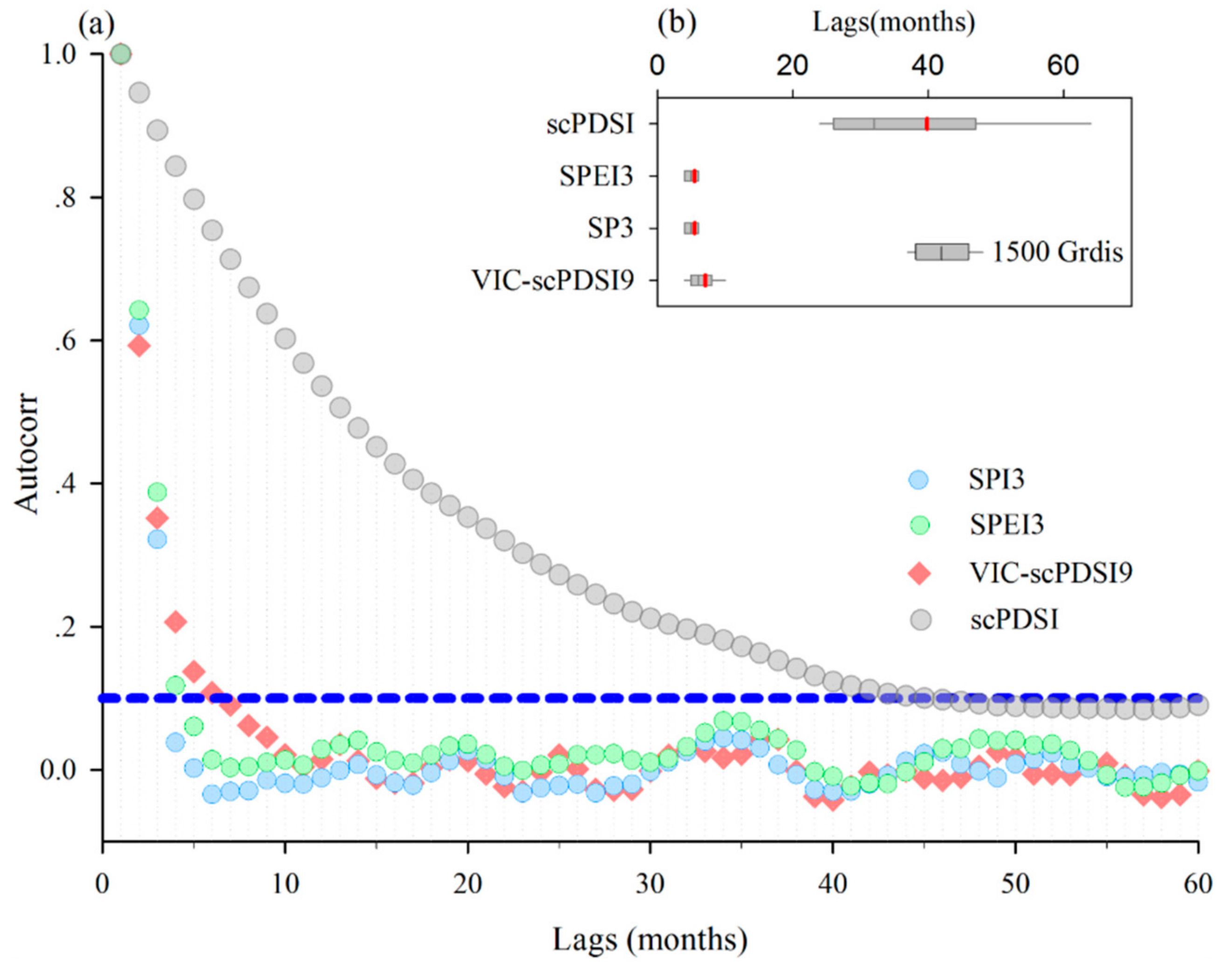
The ambiguous description on time scale is an intrinsic problem of the Palmer index family. According to the correlation analysis with SPI, it is generally accepted that PDSI is more inclined to reflect water deficiencies over a prolonged time period [35]. In an implicit manner, the time scale of scPDSI conceals in its standardization process. As shown in Figure 2, d derived from the hydrologic accounting is firstly corrected by the climatic characteristic K1 with a new Palmer variant, namely the Z index generated. Then Wells et al. [27] employed ten Z values accumulated at 3, 6, 9, 12, 18, 24, 30, 36, 42, and 48 months, respectively, to represent the extremely dry condition (the top-right panel of Figure 2). A recent literature by Liu et al. [26] found that different selections of cumulative Z values will influence the time scale of the index in a significant way. To make scPDSI capable for detecting droughts of short time scales, in this study, a new sample of cumulative Z values, accumulated at 1–9 months are used instead (the bottom-right panel of Figure 2). These 9 points are further fitted by a linear regression equation:
where t is unit of month representing the time length for accumulating Z values. m and b denote the slope and intercept of the best fit line, respectively. Xt represents the current PDSI value. C is the value of calibration index (e.g., 4, 3, …, 4). Palmer assumed that the change between any two values of Xt is constant for a given severity of drought. Based on this hypothesis, equations for computing duration factors p and q can be obtained through a complicated formula derivation process (see Wells et al. [27] for detail):
where p and q directly influence the sensitivity of the index. Larger p and smaller q means the index will be less sensitive to sudden changes in the precipitation. Palmer [11] considered that drought should be an accumulating phenomenon related to the precedent and current moisture status. With duration factors p and q, the current PDSI value Xi of ith month is expressed as the weighted sum of the precedent PDSI value Xi−1 and the current moisture anomaly Zi:
The following is the same as the original procedure of scPDSI, which involves the secondary correction with the climatic characteristic K2, and a backtracking process (the solid arrows in Figure 2).
Based on above improvements in hydrologic accounting and time scale modification, a new PDSI variant could be derived. To facilitate description, this new index is denoted as VIC-scPDSI9.
3.3. Standardized Drought Indices
The standardized precipitation index (SPI) [22] and standardized evapotranspiration precipitation index (SPEI) [15] are two representatives among the standardized drought index family which are derived from a probability distribution-based normalization procedure. In other words, mathematically SPI and SPEI follow the same algorithm and they share the same drought classification criterion. The difference mainly lies in their input. For SPI, it only considers the variation of precipitation, while for SPEI, both precipitation and potential evapotranspiration are incorporated for measuring water deficit. A fundamental strength of such standardized drought indices is that they can be computed for different time scales related to the time period of water deficiencies are accumulated. Likewise, the VIC simulated PET [34] was employed to calculate SPEI. In this study, both SPI and SPEI were cumulated at a time scale of 3-month and they were used to examine the time scale of VIC-scPDSI9.
4. Results and Discussion
4.1. Model Performance
Figure 3 compares the time series of simulated and observed daily streamflow for five selected hydrological stations situated at the upper (TNH), middle and downstream parts (WB, LM, SMX and HX) of YRB, respectively. It can be seen that both the calibration and validation periods perform very well with rather close streamflow hydrographs between simulated and observed series. With respect to the two appraisement coefficients, values of NSCE vary between 0.65 and 0.94, and the absolute values of BIAS range from 0.3% to 10.8%, suggesting that the model is capable of explaining the majority of variability in the observed data.
Figure 4 displays the spatial correlation coefficients between VIC simulated (we use the average values of top two soil layers for comparison) and observed monthly soil moisture of 57 agrometeorological sites during 1991–2008. Generally, there is a good agreement between soil moisture from these two sources with CC values mostly above 0.5. Especially in the middle parts, the CC values could reach up to 0.75. Overall, the calibrated model can replicate the hydrological process of YRB well and provide reliable estimates of hydrological variables within acceptable limits.
4.2. Time Scale and Frequency Analysis
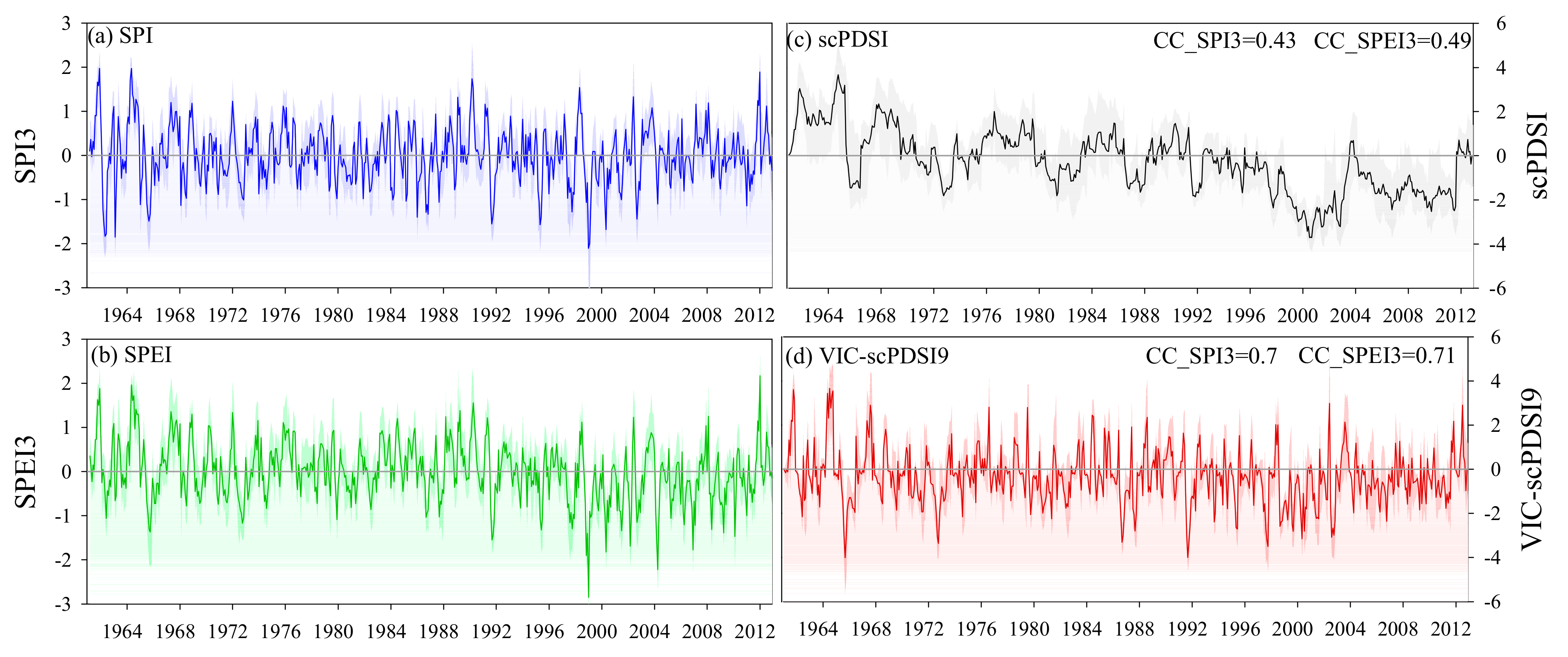
To verify the time scale of the newly generated index, the autocorrelation of monthly VIC-scPDSI9, SPI3, SPEI3, and scPDSI series was analyzed. As shown in Figure 5, the scPDSI inherently in long persistent period exhibits a rather high level of autocorrelation than the other three drought indices. The pattern of VIC-scPDSI9 by contrast, is more similar to those of SPI3 and SPEI3. For example, the autocorrelation coefficients of the three short-scalar drought indices are around 0.6 for the 1-month lag. Then, the coefficients significantly decrease and reach to a rather low value for 5-month (or even longer) lag. Figure 6 further compares the time series of the four drought indices during 1961–2012. It can be seen that the long-scalar scPDSI is less variable from month to month, and its correlation with SPI3 and SPEI3 are 0.43 and 0.49, respectively. As expected, the VIC-scPDSI9 series fluctuates in a more frequent pace, and its correlation with the two standardized indices significantly increases to 0.7. These suggest our improvement successfully changes the long time scale of original index [11,27].
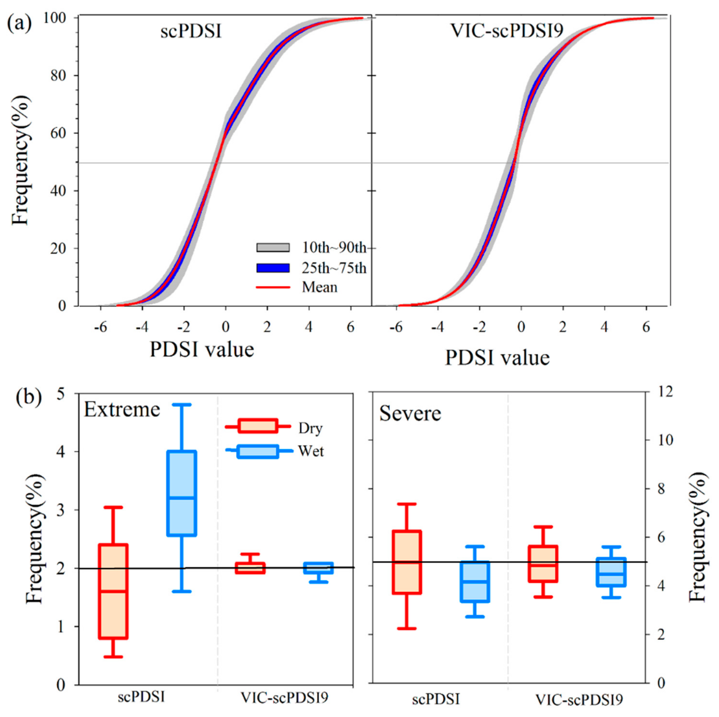
Figure 7a plots the frequency distributions of two Palmer drought indices for 1500 grids. It is seen that the VIC-scPDSI9 generally inherits the advantage of scPDSI, and behaves similarly in different areas with a rather low variance (indicated by the 75th–90th percentile range of frequency values) in the frequency of different drought categories. Minor difference between two Palmer variants mainly lies in the tails of the distribution curves for severely () and extremely () dry/wet categories. As shown in Figure 7b, the scPDSI presents an inconsistent behavior for wet and dry conditions. Especially for extreme conditions, the frequencies of wet spells are overall higher than those of dry spells. In contrast, the VIC-scPDSI9 is less variable with a frequency value of 5% for severe wet and dry spells, and 2% for extreme wet and dry spells. From a frequency perspective, the improved version is more stable than original scPDSI.
4.3. Drought Trend and Its Influencing Factors
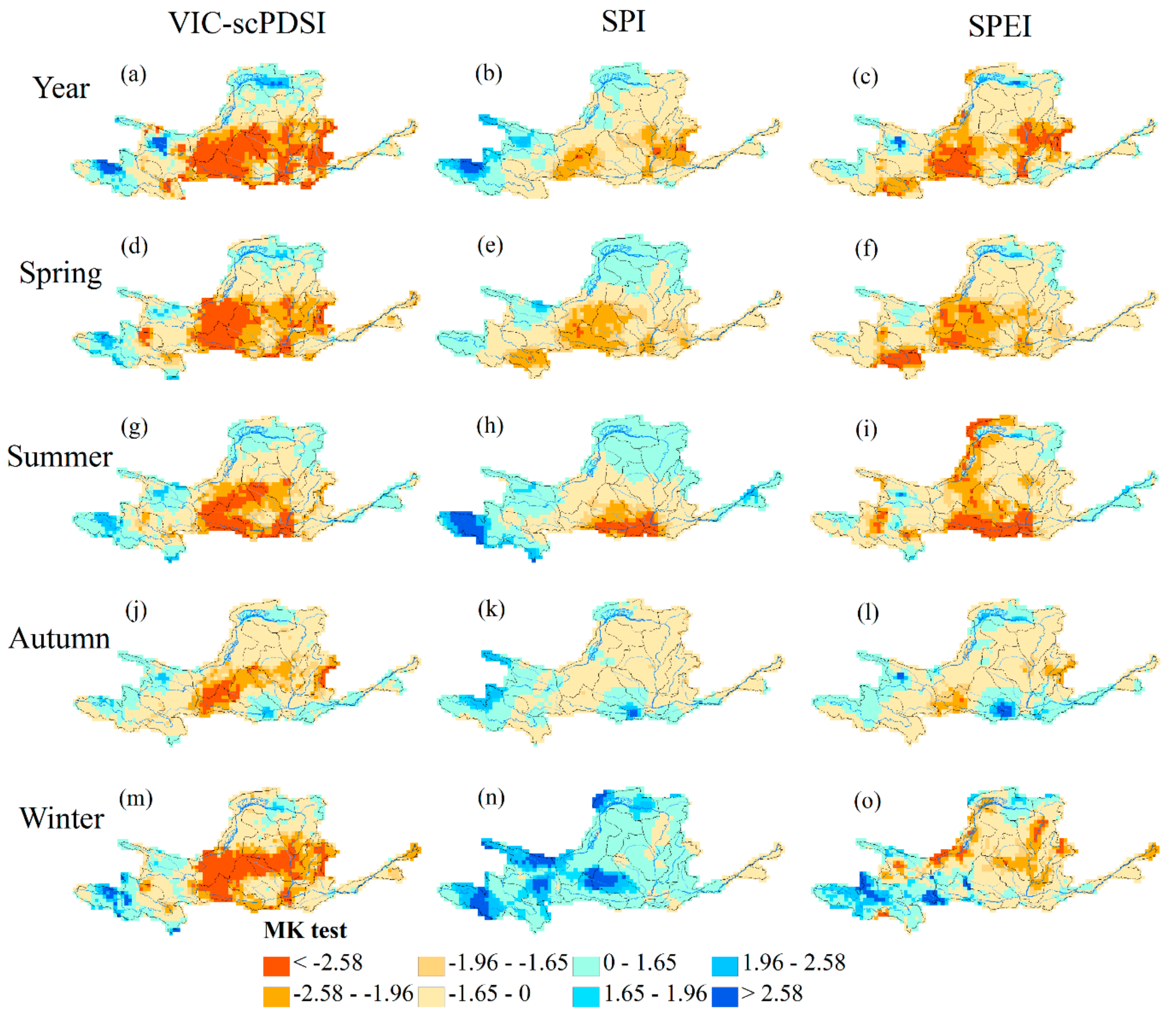
The Mann-Kendall test [36,37] was employed to detect the monotonic trend of VIC-scPDSI9, SPI3 and SPEI3 series during 1961–2012 (Figure 8). At the annual scale, a similar pattern is found between VIC-scPDSI9 and SPEI3, where both indices reflect a drying condition for the whole basin, combined with a significant (at the 1% significance level) drought tendency in the central part of YRB. For SPI3, except for the source region and northern part where the wetting status is detected, it suggests a moderate increase in dryness for the majority of the region. Patterns of spring and summer are similar to that of annual scale where a more consistent spatial distribution is observed between VIC-scPDSI9 and SPEI3. Meanwhile, the wetting area reflected by SPI3 further enlarges, especially in the northern part. In autumn, VIC-scPDSI9 indicates a significant drying pattern in the central of YRB; however, this signal is not revealed by SPI3 and SPEI3. The case of winter is very different where large differences are found among three drought indices. Overall, VIC-scPDSI9 identifies more severe drying condition than other two indices, particularly in the central of YRB. SPI3 on the contrary, indicates a wetting status over the whole basin.
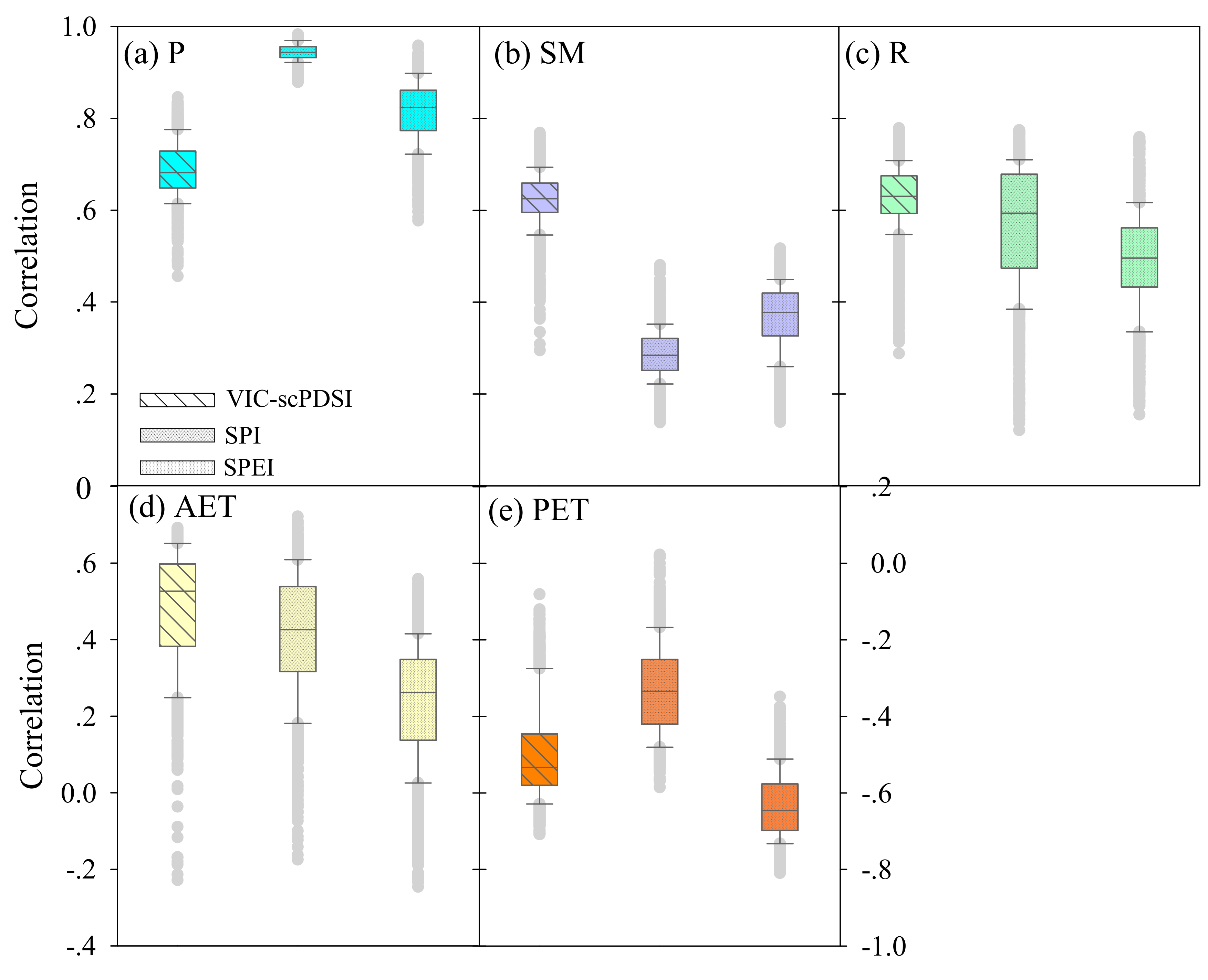
The different algorithms for estimating moisture deficits are responsible for their disparity. Given this, five crucial hydrological variables, including precipitation (P), soil moisture (SM), runoff (R), actual evapotranspiration (AET), and potential evapotranspiration (PET) were extracted to analyze their each role in drought indices. Figure 9 shows the boxplots of correlation coefficients between three drought indices and five hydrological variables. As expected, the VIC-scPDSI9 formulated from the physical constituents of water balance, shows a good correlation with all five hydrological variables (with average CC values above 0.5). Moreover, compared to the two standardized drought indices, VIC-scPDSI9 presents a better relationship with SM, R, and AET. This implies that the new Palmer variant is more inclined to reflect comprehensive moisture conditions, which could be one reason for the differential behaviors in drought trend. To verify this conjecture, Figure 10 investigates the winter trends of these five variables. It can be seen that both SM and R exhibit a drying tendency in the central zone (Figure 10d,e), which is generally in accordance with the winter pattern of VIC-scPDSI9. For SPI, precipitation is the only variable considered for depicting moisture status, thus its trend basically reflects the variation of precipitation. As shown in Figure 10a, an overall increasing tendency of precipitation in winter is apparent over whole YRB. With respect to SPEI, it generally shows equivalent correlation with P and PET, and is more inclined to reveal a coupled effect of these two variables (Figure 9 and Figure 10).
4.4. Performances in Drought Monitoring
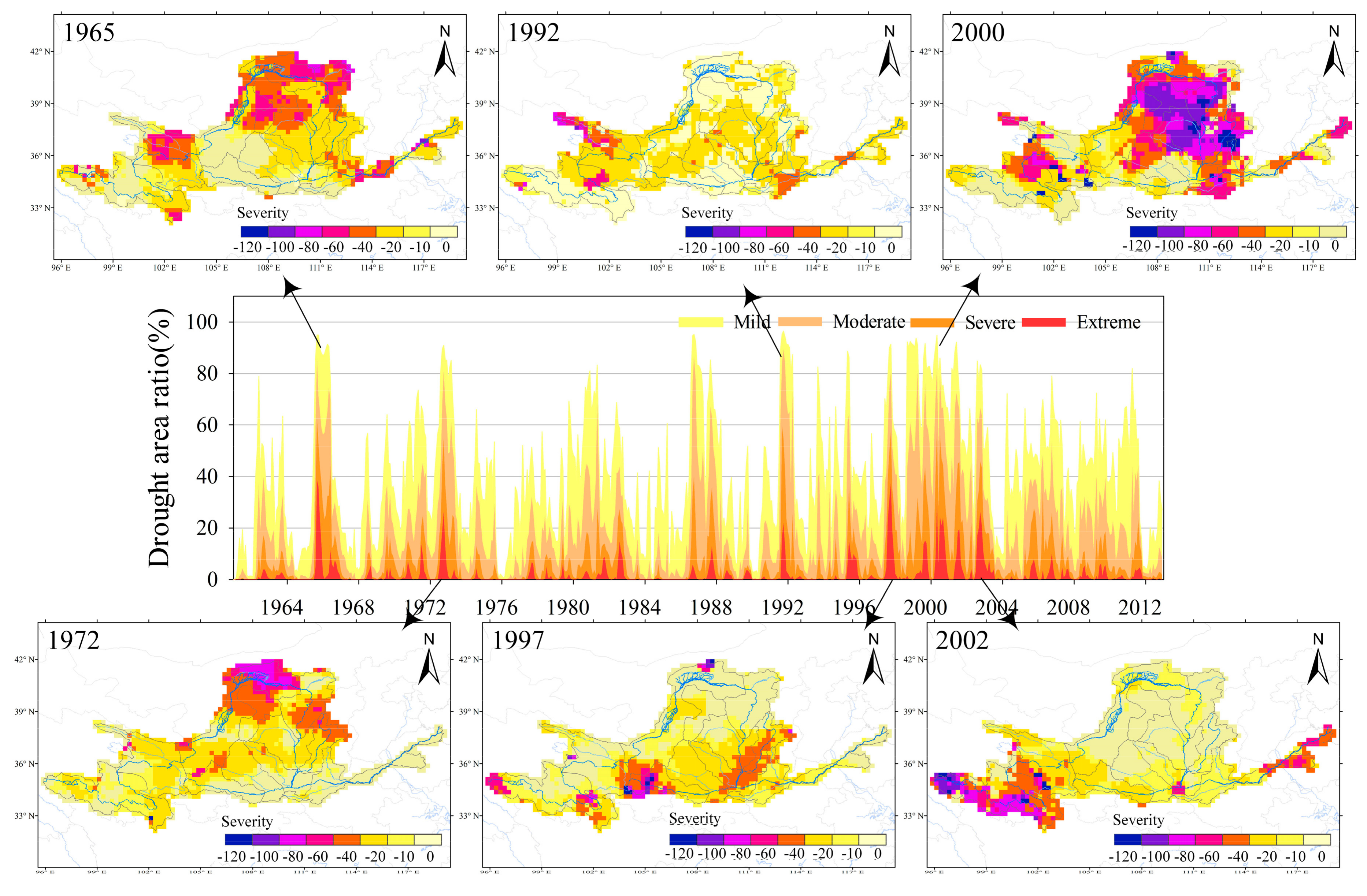
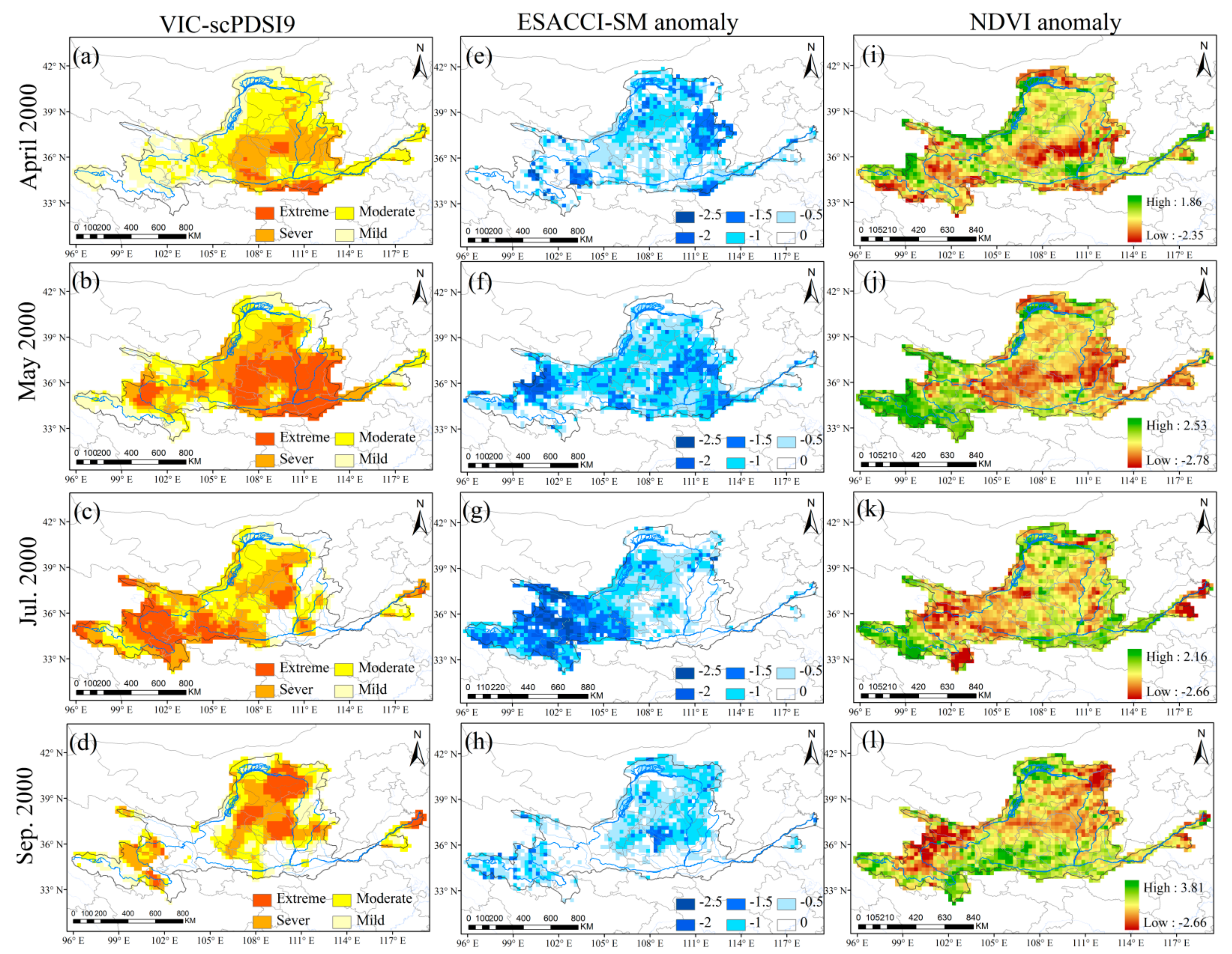
Figure 11 plots the percentage of drought area at mildly to extremely drought conditions indicated by VIC-scPDSI9. It can be seen that in each decade, the YRB may suffer at least one large-scale drought event with more than 80% of YRB affected. For instance, the 1965 drought is one typical basin-wide event, and during this period, more than 90% of the basin area is in moderate drought, 60% in severe drought, and 40% in extreme dry condition. Meanwhile, according to the distribution of accumulation severity we can see that the northern part is more vulnerable to droughts with rather high cumulative values of severity than other regions. Similar spatial distribution is also found for the 1972 drought, but the areal proportion of extreme drought is reduced to 20%. Since the 1990s, the location of drought center gradually moves toward southwest. For the 1997 drought, the southern parts are significantly drier than the northern parts, while in 2002, drought patches in large severity are mostly concentrated in the source region. Besides, the phenomenon of continuous drought events in several consecutive years also occurs during this period, and reaches to the peak (piles of drought patches with absolute accumulative values of severity exceed 100) in 2000.
To examine the performance of VIC-scPDSI9 in drought monitoring, a specific investigation on the most severe 2000 drought was conducted. Considering the short-scalar property (approximately 3-month; Figure 5 and Figure 6) of the new index, we would like to pay specific attention to its ability in monitoring the soil moisture and vegetation related drought conditions. According to the University of Maryland’s 1 km Global Land Cover Production [29], the YRB is covered by four major vegetation types: the grassland accounts for a large proportion and is mainly distributed in the source region, southern and eastern parts; the northwestern part is characterized by shrub and bare soil; in the southern and middle area, there is a small proportion of woodland; crop is mainly concentrated in the downstream of the basin. Figure 12 displays the anomalies (subtracted the mean from original series then divided by the variance) of ESACCI-SM and NDVI. The positive value of NDVI anomaly indicates a better growth condition of vegetation than the normal, and vice versa. From Figure 12 it can be seen that the VIC-scPDSI9 is capable of capturing the majority of the drought signal of ESACCI-SM anomalies and NDVI anomalies. For example, in April, all three indices reflect dryness in the central of YRB. Especially for the woodland covered areas, a more similar spatial pattern is found between VIC-scPDSI9 and NDVI anomalies. In May, the drought condition is further aggravated combined with a westward tendency. It is seen that both VIC-scPDSI9 and NDVI anomalies exhibit plies of drought patches in the middle region and crop covered downstream areas, meanwhile, the VIC-scPDSI9 and soil anomalies also reveal dryness in source region [38]. In July, the source region becomes the center of 2000 drought, as wells as for NDVI anomalies. Then the drought signal further moves northward in September. Given the general consistent behaviors with the ESACCI-SM and NDVI anomalies, it is suggested that the VIC-scPDSI9 is a good indicator for monitoring soil moisture variation and the dynamics of vegetation growth.
5. Conclusions
Based on the procedure of the self-calibrating PDSI (scPDSI), a new Palmer variant was proposed to address the shortages of coarse moisture estimation and ambiguous time scale. The improvement mainly comprises two parts: In the hydrologic accounting section, we replaced the original simplified soil moisture model with the VIC model to estimate moisture deficit/surplus. In the standardization process, we used a different sample of cumulative Z values (consist of 9 Z values accumulated at 1–9 months respectively) to calculate duration factors, aimed at changing the time scale of the index into short persistent time period. The newly generated Palmer variant is denoted as VIC-scPDSI9, and its performance was assessed over the Yellow River Basin (YRB) during 1961–2012. Two standardized drought indices SPI and SPEI at a 3-month time scale were employed as reference indices to evaluate the behaviors of the new index in aspects of time scale and drought trend. The ESA CCI soil moisture product and NDVI product were used to examine the capacity of VIC-scPDSI9 in monitoring the 2000 drought.
Results show that compared to scPDSI, the series of VIC-scPDSI9 fluctuate more frequently, and an improved relationship (correlation coefficients of 0.7) with SPI and SPEI is observed for the new variant. These confirmed our modification for making VIC-scPDSI9 of short time scales. In the aspect of drought frequency, the VIC-scPDSI9 presents a consistent pattern for wet and dry conditions, and behaves more steadily (especially for severe and extreme conditions) than the original version. We further compared the drought trend of YRB indicated by different drought indices. An overall drying condition of the whole basin, combined with a significant drought tendency in the central of this region, are found both for VIC-scPDSI9 and SPEI at the annual scale, as well as in spring and summer. The case in winter is very different, where the VIC-scPDSI9 identifies more severe drying pattern than SPI and SPEI, especially in the central of YRB. The different methods for estimating water deficits are responsible for their disparities. Since the VIC-scPDSI9 is formulated from physical constituents of water balance, this index is more inclined to reflect comprehensive moisture conditions. For the 2000 drought, the VIC-scPDSI9 can basically capture the variation of the drought signal of ESACCI-SM anomalies and NDVI anomalies, indicating the capacity of the new variant for monitoring soil moisture variation and the dynamics of vegetation growth.
With more sophisticated consideration in hydrologic accounting and the extended property of short time scales, this new Palmer variant is promising to serve as a favorable indicator for drought monitoring and assessment. In this study, the short time scale of the Palmer index was realized by using Z accumulations at 1–9 months in YRB. For other regions with different climate characteristics, one can properly adjust the sample of Z accumulations (e.g., a different combination of cumulative Z values from 1 to 10 months) to modify the time scale of the index.
Author Contributions
Y.L. designed the framework and provided software for this study. Y.Z. made substantial contributions to data processing, calculation, results analysis and wrote the manuscript. X.M. contributed to the verification of simulation results. L.R. and V.P.S. provided valuable suggestions and revised the manuscript.
Funding
This research was funded by: (1) The National Key Research and Development Program approved by Ministry of Science and Technology (Grant No. 2016YFA0601504); (2) The National Natural Science Foundation of China (Grant No. 41807165); (3) The National Natural Science Foundation of China (Grant No. 41877158); (4) The National Natural Science Foundation of Jiangsu Province, China (Grant No. BK20180512); and (5) the China Postdoctoral Science Foundation (Grant No. 2017M621615); (5) the startup Foundation for Introducing Talent of NUIST (Grant No. 2017r062).
Acknowledgments
We thank the editors and anonymous reviewers for the valuable comments and suggestions, which have helped us to improve the quality of this paper.
Conflicts of Interest
The authors declare no conflict of interest.
References
- Cook, B.I.; Smerdon, J.E.; Seager, R.; Coats, S. Global warming and 21st century drying. Clim. Dyn. 2014, 43, 2607–2627. [Google Scholar] [CrossRef] [Green Version]
- Mishra, A.K.; Singh, V.P. A review of drought concepts. J. Hydrol. 2010, 391, 202–216. [Google Scholar] [CrossRef]
- Trenberth, K.E.; Dai, A.; van der Schrier, G.; Jones, P.D.; Barichivich, J.; Briffa, K.R.; Sheffield, J. Global warming and changes in drought. Nat. Clim. Chang. 2014, 4, 17–22. [Google Scholar] [CrossRef]
- Yue, Y.; Shen, S.H.; Wang, Q. Trend and Variability in Droughts in Northeast China Based on the Reconnaissance Drought Index. Water 2018, 10, 318. [Google Scholar] [CrossRef]
- Yuan, F.; Zhang, L.; Win, K.W.W.; Ren, L.; Zhao, C.; Zhu, Y.; Jiang, S.; Liu, Y. Assessment of GPM and TRMM Multi-Satellite Precipitation Products in Streamflow Simulations in a Data-Sparse Mountainous Watershed in Myanmar. Remote Sens. 2017, 9, 302. [Google Scholar] [CrossRef]
- Sun, P.; Zhang, Q.; Yao, R.; Singh, V.P.; Song, C. Low Flow Regimes of the Tarim River Basin, China: Probabilistic Behavior, Causes and Implications. Water 2018, 10, 470. [Google Scholar] [CrossRef]
- Vicente-Serrano, S.M.; Begueria, S.; Lopez-Moreno, J.I. Comment on “Characteristics and trends in various forms of the Palmer Drought Severity Index (PDSI) during 1900–2008” by Aiguo Dai. J. Geophys. Res. 2011, 116, D19112. [Google Scholar] [CrossRef]
- Zargar, A.; Sadiq, R.; Naser, B.; Khan, F.I. A review of drought indices. Environ. Rev. 2011, 19, 333–349. [Google Scholar] [CrossRef]
- Hao, Z.; Singh, V.; Hao, F. Compound Extremes in Hydroclimatology: A Review. Water 2018, 10, 718. [Google Scholar] [CrossRef]
- Gibbs, W.J.; Maher, J.V. Rainfall deciles as drought indicators. In Bureau of Meteorology Bull. No. 48; Commonwealth of Australia: Melbourne, Australia, 1967. [Google Scholar]
- Palmer, W.C. Meteorological Drought; Weather Bureau: Washington, DC, USA, 1965; Volume 30. [Google Scholar]
- Allen, R.G.; Pereira, L.S.; Raes, D.; Smith, M. Crop Evapotranspiration: Guidelines for Computing Crop Requirements; Irrigation and Drainage Paper; Food and Agriculture Organization of the United Nations: Roma, Italy, 1998; p. 56. [Google Scholar]
- Guttman, N.B. Comparing the palmer drought index and the standardized precipitation index. J. Am. Water Resour. Assoc. 1998, 34, 113–121. [Google Scholar] [CrossRef]
- Tsakiris, G.; Pangalou, D.; Vangelis, H. Regional drought assessment based on the Reconnaissance Drought Index (RDI). Water Resour. Manag. 2007, 21, 821–833. [Google Scholar] [CrossRef]
- Vicente-Serrano, S.M.; Begueria, S.; Lopez-Moreno, J.I. A multiscalar drought index sensitive to global warming: The standardized precipitation evapotranspiration index. J. Clim. 2010, 23, 1696–1718. [Google Scholar] [CrossRef]
- Hobbins, M.T.; Wood, A.; Mcevoy, D.J.; Justin, L.H.; Morton, C.; Anderson, M.; Hain, C. The evaporative demand drought index. Part I: Linking drought evolution to variations in evaporative demand. J. Hydrometeorol. 2016, 17, 1745–1761. [Google Scholar] [CrossRef]
- Keyantash, J.A.; Dracup, J.A. An aggregate drought index: Assessing drought severity based on fluctuations in the hydrologic cycle and surface water storage. Water Resour. Res. 2004, 40, W09304. [Google Scholar] [CrossRef]
- Kao, S.C.; Govindaraju, R.S. A copula-based joint deficit index for droughts. J. Hydrol. 2010, 380, 121–134. [Google Scholar] [CrossRef]
- Liu, Y.; Zhu, Y.; Ren, L.; Yong, B.; Singh, V.P.; Yuan, F.; Jiang, S.; Yang, X. On the mechanisms of two composite methods for construction of multivariate drought indices. Sci. Total Environ. 2018, 647, 981–991. [Google Scholar] [CrossRef] [PubMed]
- Liu, Y.; Yang, X.; Ren, L.; Yuan, F.; Jiang, S.; Ma, M. A new physically based self-calibrating Palmer drought severity index and its performance evaluation. Water Resour. Manag. 2015, 29, 4833–4847. [Google Scholar] [CrossRef]
- Rajsekhar, D.; Singh, V.P.; Mishra, A.K. Multivariate drought index: An information theory based approach for integrated drought assessment. J. Hydrol. 2015, 526, 164–182. [Google Scholar] [CrossRef]
- McKee, T.B.; Doeskin, N.J.; Kleist, J. The relationship of drought frequency and duration to time scales. In Proceedings of the 8th Conference on Applied Climatology, Anaheim, CA, USA, 17–22 January 1993; pp. 179–184. [Google Scholar]
- Shukla, S.; Wood, A.W. Use of a standardized runoff index for characterizing hydrologic drought. Geophys. Res. Lett. 2008, 35, L02405. [Google Scholar] [CrossRef]
- Ma, M.; Ren, L.; Yuan, F.; Jiang, S.; Liu, Y.; Kong, H.; Gong, L. A new standardized Palmer drought index for hydro-meteorological use. Hydrol. Process. 2014, 28, 5645–5661. [Google Scholar] [CrossRef]
- Zhu, Y.; Wang, W.; Singh, V.P.; Liu, Y. Combined use of meteorological drought indices at multi-time scales for improving hydrological drought detection. Sci. Total Environ. 2016, 571, 1058–1068. [Google Scholar] [CrossRef] [PubMed]
- Liu, Y.; Zhu, Y.; Ren, L.; Singh, V.P.; Yang, X.; Yuan, F. A multiscalar Palmer drought severity index. Geophys. Res. Lett. 2017, 44, 6850–6858. [Google Scholar] [CrossRef]
- Wells, N.; Goddard, S.; Hayes, M.J. A self-calibrating Palmer drought severity index. J. Clim. 2004, 17, 2335–2351. [Google Scholar] [CrossRef]
- Zhang, H.; Singh, V.P.; Zhang, Q.; Gu, L.; Sun, W. Variation in ecological flow regimes and their response to dams in the upper yellow river basin. Environ. Earth Sci. 2016, 75, 1–16. [Google Scholar] [CrossRef]
- Hansen, M.C.; Defries, R.S.; Townshend, J.R.G.; Sohlbert, R. Global land cover classification at 1 km spatial resolution using a classification tree approach. Int. J. Remote Sens. 2000, 21, 1331–1364. [Google Scholar] [CrossRef] [Green Version]
- China Meteorological Administration (CMA). Agrometeorological Observation Specification—Soil Volume; China Meteorological Press: Beijing, China, 1993. (In Chinese) [Google Scholar]
- Dorigo, W.; Wagner, W.; Albergel, C.; Albrecht, F.; Balsamo, G.; Brocca, L.; Chung, D.; Ertl, M.; Forkel, M.; Gruber, A.; et al. ESA CCI Soil Moisture for improved Earth system understanding: State-of-the art and future directions. Remote Sens. Environ. 2017, 203, 185–215. [Google Scholar] [CrossRef]
- Liang, X.; Lettenmaier, D.P.; Wood, E.F.; Burges, S.J. A simple hydrologically based model of land surface water and energy fluxes for GCMs. J. Geophys. Res. 1994, 99, 14415–14428. [Google Scholar] [CrossRef]
- Liang, X.; Wood, E.F.; Lettenmaier, D.P. Surface soil moisture parameterization of the VIC-2L model: Evaluation and modification. Glob. Planet. Chang. 1996, 13, 195–206. [Google Scholar] [CrossRef]
- Shuttleworth, W. Handbook of Hydrology; McGraw Hill: New York, NY, USA, 1993; pp. 4.1–4.2. [Google Scholar]
- Yang, M.; Xiao, W.; Zhao, Y.; Li, X.; Lu, F.; Lu, C.; Chen, Y. Assessing Agricultural Drought in the Anthropocene: A Modified Palmer Drought Severity Index. Water 2017, 9, 725. [Google Scholar] [CrossRef]
- Mann, H.B. Nonparametric Tests against Trend. Econometrica 1945, 13, 245–259. [Google Scholar] [CrossRef]
- Kendall, M.G. Rank correlation methods. Br. J. Psychol. 1990, 25, 86–91. [Google Scholar] [CrossRef]
- Li, S.; Liang, W.; Zhang, W.; Liu, Q. Response of soil moisture to hydro-meteorological variables under different precipitation gradients in the Yellow River basin. Water Resour. Manag. 2016, 30, 1867–1884. [Google Scholar] [CrossRef]
Figure 1.
Locations of national meteorological stations, soil moisture observation sites and hydrological stations over YRB.
Figure 1.
Locations of national meteorological stations, soil moisture observation sites and hydrological stations over YRB.

Figure 2.
Flowchart of modified scPDSI’s procedure. The dashed arrows direct the computation process of PDSI, and the solid arrows denote the modifications in scPDSI. Improvement steps 1 and 2 show our improvements to the hydrologic accounting and standardization process, respectively.
Figure 2.
Flowchart of modified scPDSI’s procedure. The dashed arrows direct the computation process of PDSI, and the solid arrows denote the modifications in scPDSI. Improvement steps 1 and 2 show our improvements to the hydrologic accounting and standardization process, respectively.

Figure 3.
Daily calibration (1961–1990) and validation (1991–2012) results for five hydrological stations situated at the (a) upper, (b–e) middle and downstream parts of YRB.
Figure 3.
Daily calibration (1961–1990) and validation (1991–2012) results for five hydrological stations situated at the (a) upper, (b–e) middle and downstream parts of YRB.

Figure 4.
Spatial distribution of correlation coefficients between VIC simulated (average values of top two soil layers) and observed monthly soil moisture during 1991–2008.
Figure 4.
Spatial distribution of correlation coefficients between VIC simulated (average values of top two soil layers) and observed monthly soil moisture during 1991–2008.

Figure 5.
(a) Average autocorrelation coefficients of VIC-scPDSI9, SPI3, SPEI3 and scPDSI over YRB. The blue dashed line is the boundary (corresponding to the 0.05 significance level) of the presence of serial autocorrelation. (b) The boxplots of lagged months when the drought index series are not correlated.

Figure 6.
Time series of (a) SPI, (b) SPEI, (c) scPDSI, and (d) VIC-scPDSI9 values averaged over the whole YRB. The shadows denote the 25th–75th percentile range of index values over YRB.
Figure 6.
Time series of (a) SPI, (b) SPEI, (c) scPDSI, and (d) VIC-scPDSI9 values averaged over the whole YRB. The shadows denote the 25th–75th percentile range of index values over YRB.

Figure 7.
(a) Frequency distributions of scPDSI and VIC-scPDSI9 values. The grey and blue shadows denote the 75th–90th percentile range of frequency values over YRB. (b) The boxplots of scPDSI and VIC-scPDSI9 values of 1500 grids at extremely and severe dry levels.
Figure 7.
(a) Frequency distributions of scPDSI and VIC-scPDSI9 values. The grey and blue shadows denote the 75th–90th percentile range of frequency values over YRB. (b) The boxplots of scPDSI and VIC-scPDSI9 values of 1500 grids at extremely and severe dry levels.

Figure 8.
Spatial distribution of MK test statistics for annual and seasonal index values of VIC-scPDSI9 (left column), SPI3 (middle column), and SPEI3 (right column), respectively. The absolute values of MK statistics of 2.576, 1.96 and 1.645 correspond to the 1, 5 and 10% significance levels, respectively.

Figure 9.
The boxplots of correlation coefficients between VIC-scPDSI9, SPI3, SPEI3 against five hydrological variables.
Figure 9.
The boxplots of correlation coefficients between VIC-scPDSI9, SPI3, SPEI3 against five hydrological variables.

Figure 10.
Spatial distribution of the winter trends for five hydrological variables.

Figure 11.
Time series of drought area at mildly to extremely dry levels by VIC-scPDSI9. The small rectangle panels show the spatial distribution of accumulated drought severity for six typical drought events.
Figure 11.
Time series of drought area at mildly to extremely dry levels by VIC-scPDSI9. The small rectangle panels show the spatial distribution of accumulated drought severity for six typical drought events.

Figure 12.
Spatial evolution of the 2000 drought indicated by (a–d) VIC-scPDSI9, (e–h) ESACCI anomaly, and (i–k) NDVI anomaly.
Figure 12.
Spatial evolution of the 2000 drought indicated by (a–d) VIC-scPDSI9, (e–h) ESACCI anomaly, and (i–k) NDVI anomaly.


Table 1.
Information on the 10 hydrological stations of the Yellow River Basin.
| Hydrological Station | Abbreviation | Longitude (°E) | Latitude (°N) | Digital Elevation Model (m) | Drainage Area (104 km2) | Areal Average Precipitation (mm/year) |
|---|---|---|---|---|---|---|
| Tangnaihai | TNH | 100°09′ | 35°30′ | 2960 | 12.2 | 520.8 |
| Lanzhou | LZ | 103°49′ | 36°04′ | 1774 | 10.07 | 480.7 |
| Toudaoguai | TDG | 111°04′ | 40°16′ | 1000 | 14.53 | 390.9 |
| Wubao | WB | 110°43′ | 37°27′ | 960 | 6.56 | 394.5 |
| Longmen | LM | 110°35′ | 35°40′ | 393 | 6.24 | 402.2 |
| Hejin | HJ | 110°48′ | 35°34′ | 553 | 12.21 | 485.7 |
| Xianyang | XY | 108°42′ | 34°19′ | 406 | 10.07 | 555.1 |
| Huaxian | HX | 109°46′ | 34°35′ | 481 | 14.53 | 544.3 |
| Sanmenxia | SMX | 111°22′ | 34°49′ | 614 | 4.75 | 398.2 |
| Huayuankou | HYK | 113°39′ | 34°55′ | 106 | 4.18 | 440.2 |
© 2018 by the authors. Licensee MDPI, Basel, Switzerland. This article is an open access article distributed under the terms and conditions of the Creative Commons Attribution (CC BY) license (http://creativecommons.org/licenses/by/4.0/).
Share and Cite
MDPI and ACS Style
Zhu, Y.; Liu, Y.; Ma, X.; Ren, L.; Singh, V.P. Drought Analysis in the Yellow River Basin Based on a Short-Scalar Palmer Drought Severity Index. Water 2018, 10, 1526. https://doi.org/10.3390/w10111526
AMA Style
Zhu Y, Liu Y, Ma X, Ren L, Singh VP. Drought Analysis in the Yellow River Basin Based on a Short-Scalar Palmer Drought Severity Index. Water. 2018; 10(11):1526. https://doi.org/10.3390/w10111526
Chicago/Turabian StyleZhu, Ye, Yi Liu, Xieyao Ma, Liliang Ren, and Vijay P. Singh. 2018. "Drought Analysis in the Yellow River Basin Based on a Short-Scalar Palmer Drought Severity Index" Water 10, no. 11: 1526. https://doi.org/10.3390/w10111526
Note that from the first issue of 2016, this journal uses article numbers instead of page numbers. See further details here.