An Integrated Modeling Approach to Study the Surface Water-Groundwater Interactions and Influence of Temporal Damping Effects on the Hydrological Cycle in the Miho Catchment in South Korea

Abstract

Integrated surface water–groundwater (SW–GW) models could be used to assess the impacts of climate change or variability on the hydrological cycle. However, the damping effects of the hydrological system have rarely been explored via integrated SW–GW modeling. This paper presents an integrated modeling study in a typical humid area, the Miho catchment in Korea, using an integrated model called Groundwater and Surface-water FLOW (GSFLOW). The major findings of this study are as follows: (1) The simulated results from 2005 to 2014 indicate that the temporal variability in the streamflow, stream-groundwater interactions and groundwater recharge are dominated by the precipitation, while the temporal variability in the evapotranspiration (ET) is controlled by the energy conditions; (2) Damping effects can affect the hydrological cycle across different temporal and spatial scales. At the catchment scale, the soil zone and aquifer play a dominant role in damping the precipitation on monthly and annual time scales, respectively; (3) Variability in the capacity to buffer earlier precipitation is found at small spatial scales, such as streams, and larger spatial scales, such as the whole catchment. This variability could affect the water balance at larger spatial scales and affect the hydrography recession at smaller spatial scales.

1. Introduction

The hydrologic cycle describes the continuous movement of water on Earth [1]. Knowledge of the hydrologic cycle plays a vital role in water resources management. In the hydrologic cycle, water storage is one of the key hydrological components that connects the SW–GW. However, it is a challenging task to estimate the total water storage in a catchment, due to their heterogeneity of the system and the difficulty to measure the system properties and system states [2]. Despite their importance, surface water (SW) and groundwater (GW) are usually analyzed as two separate domains because their processes occur on different time scales, and it is challenging to measure their interactions [3,4]. To better understand the hydrologic cycle, lots of efforts have been made to develop physically-based integrated hydrological models (IHMs); e.g., InHM [5], MIKE-SHE [6,7], Hydrogeosphere [8], PARFLOW [9], SWAT-MODFLOW [10], MODHMS [11], GSFLOW [12] and others. However, the initial applications of these models have been limited to experimental plots or relatively small catchments. For these models to draw attention from the hydrological community, it must be demonstrated that IHMs are capable of simulating hydrological process at larger scales [13]. In the last few years, IHMs at larger scales have been increasingly used in water resources management. Jones et al. [13] attempted to assess the ability of IHM to simulate the transient flow process at a larger scale. Hassan et al. [14] used the GSFLOW model to assess the effect of hard rock systems on surface water–groundwater (SW–GW) interactions in a semi-arid hilly catchment in Spain. Tian et al. [15] established an integrated SW–GW model for an inland river basin in China using GSFLOW to explore scale-dependent ecohydrological process. Seyoum and Milewski [16] used an IHM to characterize terrestrial water storage anomalies. These studies enhanced our understanding of the entire basin-scale water cycle and variability in the hydrologic response. However, few investigations have been conducted to study the influence of the temporal variability and damping effects, especially the influence of precipitation [17].

A hydrological system involves slow variables (e.g., interflow, groundwater flow) in the subsurface domain (i.e., vadose zone and aquifer) and fast variables in the surface domain (e.g., precipitation, streamflow). As a result, hydrological processes inherently operate over many time scales [18]. Furthermore, due to the delayed response in the hydrological system of the subsurface domain, the time dependencies of hydrological catchment responses to precipitation may range from daily to annual time scales. The delayed response is defined here as damping effects. The damping effect of a hydrological system is also reflected in the fluctuation in its storage, which acts as a buffer between the water inputs and streamflow response. This buffer capacity is also recognized as catchment memory. Many studies noted the importance of catchment memory and studied the role of storage on current and future responses to anticipated climate changes [19,20,21]. Understanding the variability in buffering capacity is also highly relevant for water resource managers who want to develop a long-term drought management strategy. Integrated SW–GW models provide an ideal tool to evaluate times scales and damping effects; nevertheless, they have rarely been used to explore these issues.

In South Korea, the water resources management is generally concentrated on the development of surface water resources. Fewer groundwater studies have been performed than surface water studies [22]. In the past few decades, water scarcity problems have increased due to climate change. Thus, numerous researchers have drawn attention to the interactions of surface water and groundwater to improve conjunctive water management [23]. Integrated SW–GW modeling has been attempted in several basins. For example, SWAT–MODFLOW has been used to study river-aquifer interactions and to estimate the spatial-temporal distribution of groundwater recharge rates and aquifer evapotranspiration (ET) for several basins in South Korea [10,24]. However, these studies focused on the role of spatial variability in the SW–GW interactions.

This study presents the calibration and verification of a GSFLOW (Version 1.1.6, U.S. Geological Survey, Reston, VA, USA) model for the Miho catchment in Korea. GSFLOW is selected because the PRMS and MODFLOW are widely employed for surface water and groundwater analyses by practicing hydrologist in South Korea [25,26,27,28]. In addition, these two models have similar modular programing methods, and GSFLOW can be integrated to simulate other environmental and anthropogenic impact. Thus, applying the GSFLOW model will be beneficial for the water resource management and research in South Korea. [12]. The Miho catchment is in the headwaters of the Geum River basin. Floods are of major concern in the study area. However, droughts have become more frequent and more serious in the last decade [29,30]. Therefore, substantial attention has been drawn to the water scarcity issue. In recent years, event-based flood simulation and distributed hydrological modeling have been carried out in the study area [23], but fully integrated SW–GW modeling has not been attempted. A coherent understanding of the catchment water cycle and its interconnection with water scarcity has yet to be determined.

This study aims to: (1) elucidate the dynamics of the SW–GW interactions and provide a long-term, quantitative water balance of a humid catchment; (2) investigate the influence of temporal variability and damping effects on the hydrological processes; and (3), generate insights into tackling water resources management.

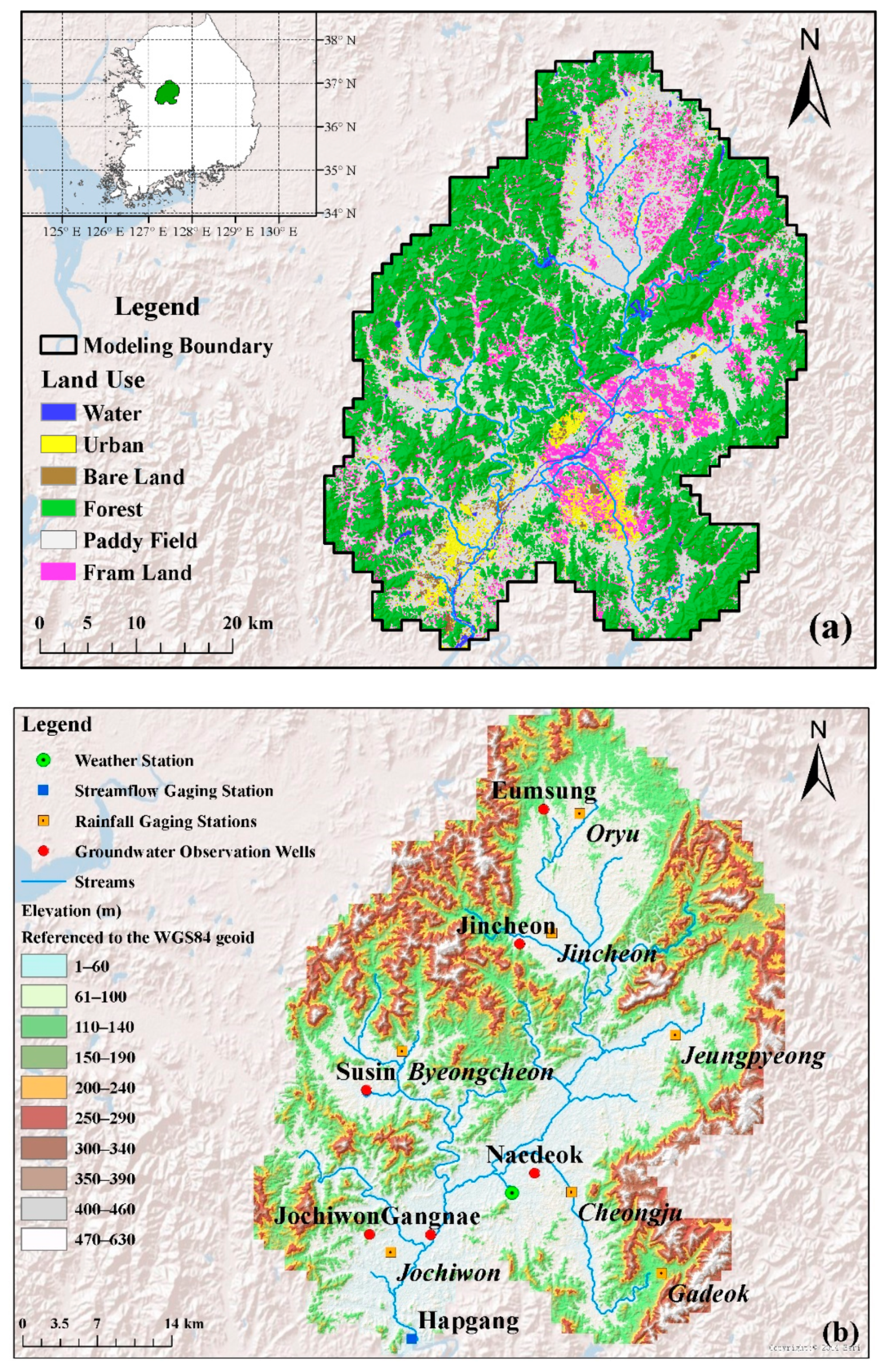
2. Study Area and Data

Our study area, the Miho catchment (Figure 1), is in the headwaters of the Geum River basin, which drains the central part of the Korean peninsula. The Miho stream originates from Mt. Mangisan, and flows through Jincheon-gun, Jeungpyeong-gun, Cheongju-si, and Sejong-si. The population of the Miho catchment was approximately one million in 2011. The catchment drains an area of approximately 2100 km², and its elevation ranges from 7 to 631 m (Figure 1b). The length of the Miho stream is approximately 97 km, and the annual areal discharge is approximately 600 mm. The climatic characteristic of this area is distinct dry (October to May) and wet (June to September) seasons. The average temperatures in the Miho catchment during the dry and wet seasons are 6.9 degrees Celsius and 23.6 degrees Celsius, respectively. The total precipitation during the dry season is 380.1 mm, while the total precipitation during the wet season is 859 mm, according to meteorological observations from 1981 to 2010 provided by the Korea Meteorological Administration (KMA, http://www.kma.go.kr). Approximately 70% of the annual precipitation (1239 mm) falls during the wet season.

The main aquifers of the Miho catchment are composed of granite, schist, gneiss, and alluvium [24,31]. In the upper portion of the Miho catchment, such as in Jincheon and Eumsung, the aquifer system is generally composed of unconsolidated sediments, Cretaceous volcanic rocks, Cretaceous sedimentary rocks, and paragneiss. The middle portion of the Miho catchment consists of Cretaceous sedimentary rocks, Triassic–Jurassic acidic intrusive igneous rocks, and paragneiss. The downstream area consists of Jurassic acidic intrusive igneous rocks, low-grade metamorphic rocks, and paragneiss [31,32,33,34].

A variety of data have been collected for establishing and calibrating the Miho GSFLOW model. The data are roughly grouped into three categories. The first category is the data for the model setup and initial parameterization. Gridded datasets of elevation, geology, vegetation, soil, and land use were collected and processed to establish and parameterize the GSFLOW model. These datasets include a digital elevation model (DEM) with a spatial resolution of 30 m, a landuse map in 2000 and soil maps of the physical properties of the soil layer (texture, available water capacity, saturated conductivity, etc.). The DEM was retrieved from the ASTER DEM (http://asterweb.jpl.nasa.gov). The digital land use and soil maps were obtained from Water Resources Management Information System (WAMIS, http://www.wamis.go.kr). Figure 1a shows the distribution of the land use. It can be seen that approximately half of the Miho catchment is covered by forest (55.1%), which is mainly distributed over the mountain areas. The rest of the area consists of paddy fields (16.2%), farmlands (11.4%) and urban areas (9.1%). The soil type is dominated by silty, clayey loam, clayey and sandy soils. The mountain areas generally consist of coarse silty or clayey loam soils, the flatlands consist of clayey loam or clayey soils, and the riparian areas are mainly composed of coarse silty or sandy soils.

The second data category is meteorological data, including precipitation, temperature (maximum, minimum and average), air pressure, relative humidity, wind speed, and sunshine hours, used to drive the model. Daily meteorological data measured at one weather-gauging station (Cheongju weather station) and seven rainfall-gauging stations from 2004 to 2014 were obtained from WAMIS and KMA. In fact, there are nine rainfall-gauging stations in the study area. However, considering the data quality and recording periods, only seven of the stations were used in this study (in Figure 1b).

The last data category includes hydrological observations for the model calibration and validation (from 2004 to 2014). Daily streamflow observations measured at the Hapgang gaging station (in Figure 1b), the outlet station of the study area, were obtained from WAMIS. Daily groundwater heads measured at seven national observation wells (in Figure 1b) were retrieved from the Groundwater Information Service (GIMS, http://www.gims.go.kr).

3. Methods

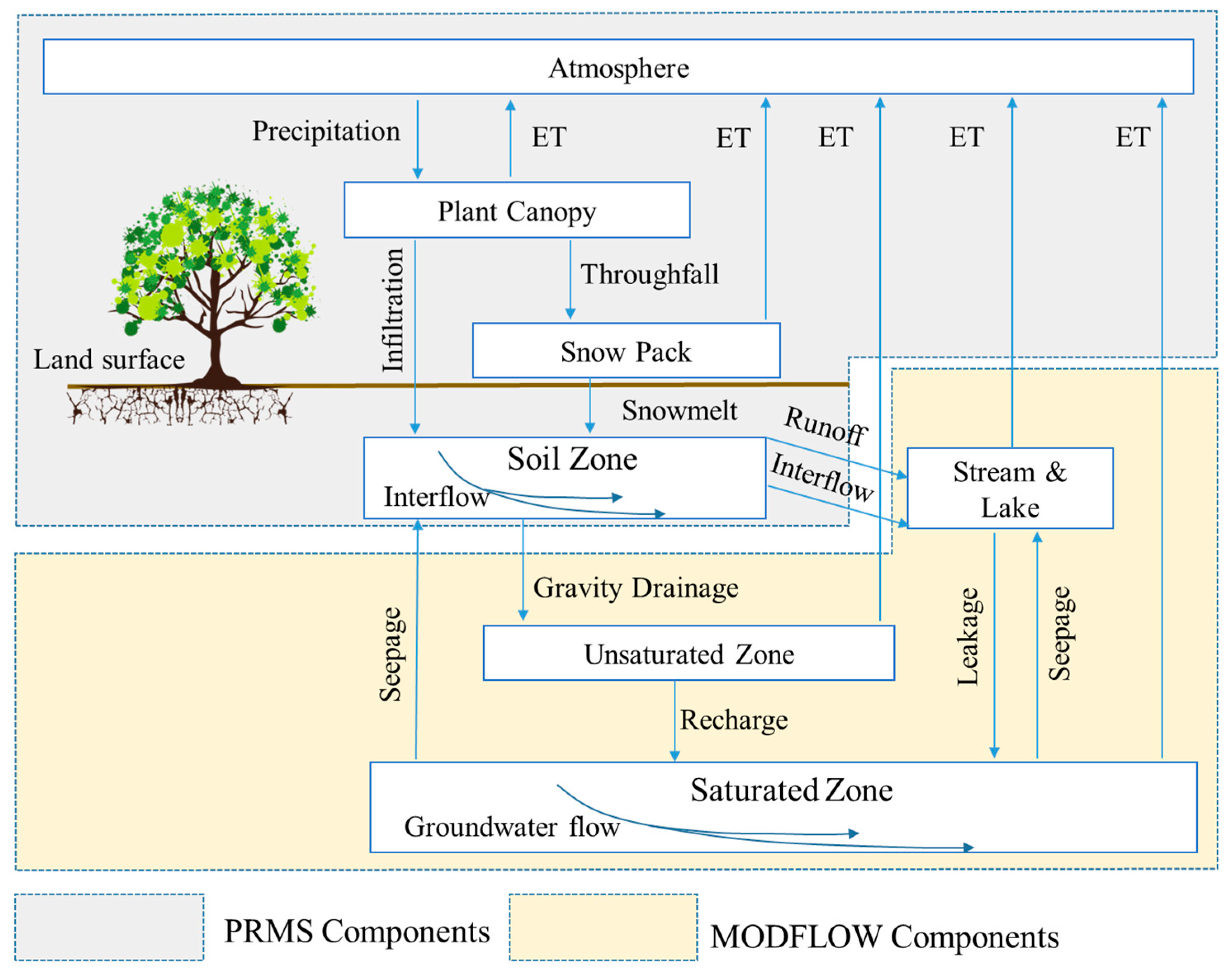
3.1. Introduction to GSFLOW

GSFLOW provides a comprehensive system for simulating all the major processes of the hydrologic cycle. Figure 2 demonstrates schematic diagram of GSFLOW. GSFLOW integrates the Precipitation-Runoff Modeling System (PRMS) (Version 3.0.5, U.S. Geological Survey, Reston, VA, USA) [35] with the Modular Ground-Water Flow Model (MODFLOW-2005) (Version 1.9.1, U.S. Geological Survey, Reston, VA, USA) [36], which simulate surface hydrology (top of the plant canopy to the soil zone base) and 3-D groundwater (the base of the soil zone to the base of the aquifers), respectively [12]. In the surface domain, hydrologic response units (HRUs) are the basic computing units, which can be either regular grids or irregular polygons. In the subsurface, the aquifer is discretized with finite difference grids. In the surface domain, GSFLOW uses a cascade method to route the overland flow and interflow among the HRUs and to the streams and lakes. Cascade flow paths are determined from the elevations of each HRU. Cascade paths can cross any of the four faces of an HRU to a stream or to a lake within or adjacent to an HRU. Cascades can terminate at a stream, lake, or HRU that has been designated as a watershed outflow location. The flow path among the HRUs and the fraction of the area in the upslope HRUs that contributes flow to the downslope HRUs are predefined rather than computed in real-time. This mass-balance-based method avoids numerical oscillation and saves considerable computation time, compared with strictly physically-based models (e.g., Parflow), since it can use a rather long time step (e.g., daily). The detailed about the cascade method of GSFLOW are well described in The U.S. Geological Survey Cascade Routing Tool (CRT) [37]. Considering computation costs, this method seems to be more applicable for large-scale basin modeling, although the simulation of surface flow is simplified.

To simulate the two-way interactions between the surface water and groundwater, GSFLOW defines a “gravity reservoir” as a storage area in which an HRU exchanges water with the MODFLOW grid(s) it intersects. GSFLOW defines an unsaturated zone between the soil zone and the aquifer. This unsaturated zone is simulated using the Unsaturated Zone Flow package (UZF1) [38]. Streams and lakes are simulated using the Streamflow Routing package (SFR2) [39] and Lake package [40], respectively. In reaches where the stream water is connected to the groundwater, the stream–aquifer exchange is calculated based on the head difference using Darcy’s law. More details on GSFLOW can be found in Markstrom et al. [12]. An improved version of GSFLOW was developed by Tian et al. [41], who improved the ET calculation by using the FAO Penman–Monteith (FAO–PM) method. This improved version was adopted in this study.

3.2. Model Setup

Setup of the Miho GSFLOW model was accomplished with the aid of Visual Hydrological-Ecological Integrated watershed-scale Flow (Visual HEIFLOW), which was developed by Tian et al. [42]. The main procedures of the setup are described below.

3.2.1. Model Domain Decomposition

Watershed delineation was first performed to generate the model domain boundary, subbasins and stream network. The delineation was accomplished by using the Terrain Analysis Using Digital Elevation Models (TauDEM) library [43], which was embedded in the VHF. Then, the model domain was discretized into regular grids. Uniform grids were used for both the surface and subsurface domains. Each grid cell in the surface domain represents an individual HRU. The uniform grids are beneficial for reducing computation errors when coupling with a groundwater model because each HRU is directly linked with a subsurface finite difference grid cell.

As shown in Figure 3, the surface model domain was delineated into 51 subbasins and 2141 grid cells with 1 × 1 km cell size. In GSFLOW, the stream network is divided into reaches and segments. The stream network is composed of 51 segments and 461 reaches. A reach is a section of a stream that connects to a particular MODFLOW grid [12]. A segment is a group of reaches that have uniform or linearly changing properties and other uniform characteristics (e.g., Manning’s roughness coefficient). In addition to the delineation and discretization, geometric parameters related to the grid cells and streams were also calculated. The DEM was used to define the top elevation of the MODFLOW grids and streambed within the Miho catchment. Finally, the Cascade Routing Tool (CRT), developed by Henson et al. [37], was used to calculate the flow routing of the study area.

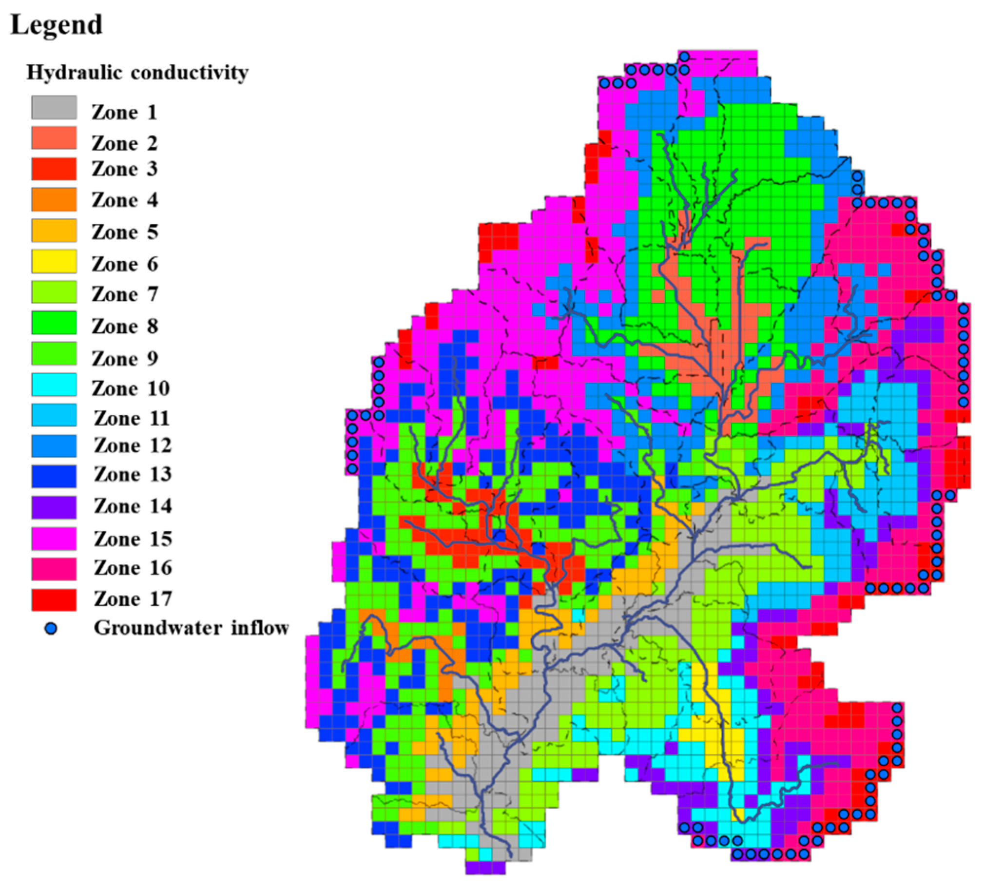
3.2.2. Surface and Subsurface Model Parameterization

In the surface domain, the spatially distributed parameters of the HRUs were initially estimated from data such as the DEM, land use type, soil data, and vegetation data. The initial HRU parameter sets were further adjusted during model calibration. The subsurface was divided into three layers, each with 2141 active cells. The first and the third layers represent a shallow unconfined aquifer and deeper confined aquifer, respectively, while the second layer represents an aquitard. The key parameters of the subsurface model in this study include the horizontal hydraulic conductivity (HK), vertical hydraulic conductivity (VK), specific storage (SR), and specific yield (SY). To facilitate parameterization, the subsurface domain was divided into 17 parameter zones based on the topographical location, geology, and rock types, as shown in Figure 3. An initial assessment and possible range for each of these parameters were estimated according to borehole data, geologic and hydrogeologic reports, and previous studies [10,24]. Based on previous studies [24] and published reports from South Korean government agencies [31,32,33,34], specified flow conditions were applied along part of the boundary, as indicated by the blue dots in Figure 3. During the model calibration, the total amount of inflow was tuned within a pre-estimated range to ensure adequate groundwater head simulations. Since no information on the temporal variability in the inflow is available, time-invariant daily inflow rates were assumed.

Due to a lack of geometric information on the stream cross sections, rectangular cross sections were assumed for all segments of the stream network. The widths of the cross sections were estimated from Geographic Information System (GIS) data and Google Earth images. The streambed hydraulic conductivities and Manning’s roughness coefficients were set according to information from the field surveys and previous studies [24,31,32,33,34]. The properties of the unsaturated zone beneath all the stream reaches were constant: a vertical hydraulic conductivity of 0.3 m/d, a saturated water content of 0.30 and a Brooks–Corey exponent of 3.5 [39].

3.2.3. Generation of Driving Forces

The meteorological data observed at the Cheongju weather station was assumed to be representative of the whole Miho catchment. The observed precipitation at the seven rainfall-gauging stations was interpolated to each HRU using the inverse distance weighting (IDW) method. The potential ET (PET) was calculated using the FAO-PM method. Due to a lack of information on the groundwater withdraws, groundwater pumping was ignored in this study.

3.3. Model Calibration

The model was calibrated using a stepwise procedure: First, the MODFLOW model was calibrated independently of PRMS under a steady-state stress period, followed by calibration of the integrated model under transit-state stress periods. The calibration of the steady state groundwater simulation was accomplished by identifying a set of aquifer hydraulic conductivity values, hydrologic stresses and boundary conditions so that the simulated groundwater heads matched the observed values to a reasonable degree, considering the average conditions from 2000 to 2004.

The integrated model calibration under the transient stress periods was performed through several trial and error procedures. The parameters that affect major components of the water budget and fluxes of water across different regions were adjusted until the model provided a reasonable water balance. Then, records of the daily streamflow and groundwater heads were used to calibrate the model. The PRMS model parameters, mainly related to the surface runoff and soil-zone modules, were adjusted by considering the physical constraints. For example, the calibrated parameter of the maximum volume of water per unit area in the capillary reservoir (soil_moist_max) indicated a range from 5 inches to 18 inches.

To properly calibrate the groundwater model under the transient stress period, a good estimation of the hydraulic conductivities and boundary conditions from the steady state calibration was required. The specific yield for the unconfined aquifer and storage coefficient for the confined aquifer were mainly calibrated during the transient stress period. These parameters were adjusted until acceptable matches were obtained between the observed and simulated groundwater head fluctuations. Meanwhile, the parameters related to the stream–aquifer interactions were carefully adjusted, until the model not only provided a good fit between the measured and observed streamflow but also reproduced the spatial and temporal patterns of river–aquifer interactions revealed by existing studies. The model performance of the streamflow simulation was evaluated by determining the Nash-Sutcliffe efficiency (NSE) and coefficient of determination (R²). NSE and R² tend to give more weightage to the high-magnitude flows. Another two error statistics based on percentage error in simulation with respect to observed value, including threshold statistics (TS), average absolute relative error (AARE). The model performance of the groundwater simulation was evaluated by determining the root-mean-square error (RMSE).

Table 1. Calibrated parameter ranges for the Miho GSFLOW model.

Zone	Parameters	Minimum	Maximum	Unit	Model
Surface	covden_sum	0.1	0.9	dimensionless	PRMS
	covden_win	0	0.1	dimensionless	PRMS
	srain_intcp	0	0.05	inches	PRMS
	wrain_intcp	0.1	3	inches	PRMS
	snow_intcp	0.1	3	inches	PRMS
Soil	soil_moist_max	5	18	inches	PRMS
	soil_moist_init	0.5	9	inches	PRMS
	soil_rechr_max	3	9	inches	PRMS
	soil_rechr_init	0.5	4.5	inches	PRMS
Groundwater	HK (layer 1)	0.5	10	meters per day	MODFLOW
	HK (layer 2)	0.1	2	meters per day	MODFLOW
	HK (layer 3)	0.02	0.4	meters per day	MODFLOW
	VK (layer 1)	0.0083	0.33	meters per day	MODFLOW
	VK (layer 2)	0.00014	0.0056	meters per day	MODFLOW
	VK (layer 3)	2.3 × 10−5	0.0009	meters per day	MODFLOW
	SY	0.04	0.11	dimensionless	MODFLOW
	SS	1.0 × 10−5	4.0 × 10−5	meters−1	MODFLOW

presents the ranges of the calibrated key parameter values. The equations to compute these statistics are presented below.

$$\mathrm{NSE}=1-\frac{{{\displaystyle \sum }}_{t=1}^N{(Q_m^t-Q_o^t)}^2}{{{\displaystyle \sum }}_{t=1}^N{(Q_o^t-\overline{Q_o})}^2}$$

(1)

$${\mathrm{R}}^2=\frac{{{\displaystyle \sum }}_{t=1}^N(Q_o^t-\overline{Q_o})(Q_m^t-\overline{Q_m})}{\sqrt{{{\displaystyle \sum }}_{t=1}^N{(Q_o^t-\overline{Q_o})}^2}\sqrt{{{\displaystyle \sum }}_{t=1}^N{(Q_m^t-\overline{Q_m})}^2}}$$

(2)

$$AARE=\frac{1}{N}{\displaystyle \sum }_{t=1}^N|R{E}_t|$$

(3)

$$R{E}_t=\frac{Q_m^t-Q_o^t}{Q_o^t}\times 100\%$$

(4)

$$T{S}_x=\frac{n_x}{N}\times 100\%$$

(5)

$$RMSE=\sqrt{\frac{1}{N}{\displaystyle \sum }_{t=1}^N{(Q_m^t-Q_o^t)}^2}$$

(6)

where $Q_m^t$ is simulated flow at time t; $Q_o^t$ is observed flow at time t; $\overline{Q_o}$ is the mean of observed flow; $\overline{Q_p}$ is the mean of observed flow; $R{E}_t$ is the relative error in simulation; $n_x$ is the total number of flow data points predicted in which the absolute relative error (ARE) in simulation is less than x%; and N is the total number of flow data points simulated.

3.4. Water Balance Analysis

The water balance of the Miho catchment was calculated for the entire study area based on the GSFLOW model simulation results. The water balance can be described by the following equation:

$$\mathrm{P}+{\mathrm{GW}}_{in}=\mathrm{ET}+\mathrm{Q}+{\mathrm{GW}}_{out}+\Delta \mathrm{S}$$

(7)

where P is the precipitation; ${\mathrm{GW}}_{in}$ represents the groundwater inflow; ET is the total evapotranspiration; $Q$ and ${\mathrm{GW}}_{out}$ are the surface water outflow and lateral groundwater outflow across the model boundary, respectively; and $\Delta \mathrm{S}$ is the total storage change.

The total ET can be further decomposed as follows:

$$\mathrm{ET}={\mathrm{E}}_{sf}+{\mathrm{ET}}_{sz}+{\mathrm{ET}}_{uz}+{\mathrm{ET}}_{sat}$$

(8)

where ${\mathrm{E}}_{sf}$ is evaporation from the surface zone, including evaporation of intercepted precipitation, evaporation from impervious areas and snow sublimation; ${\mathrm{ET}}_{sz}$, ${\mathrm{ET}}_{uz}$ and ${\mathrm{ET}}_{sat}$ are the subsurface ET components, regarding the soil zone, unsaturated zone and saturated zone, respectively.

The streamflow at the catchment outlet ($\mathrm{Q}$) can be expressed as follows:

$$\mathrm{Q}={\mathrm{HR}}_{riv}+{\mathrm{DR}}_{riv}+{\mathrm{q}}_{g2s}-{\mathrm{q}}_{s2g}$$

(9)

where ${\mathrm{HR}}_{riv}$ is the Hortonian runoff, which is simulated as an infiltration excess of precipitation at the land surface and is routed to the streams; ${\mathrm{DR}}_{riv}$ is the soil zone interflow that reaches the streams; ${\mathrm{q}}_{g2s}$ is the groundwater discharge to the streams; and ${\mathrm{q}}_{s2g}$ is the stream leakage to the groundwater.

The total storage change $\Delta \mathrm{S}$ is computed as follows:

$$\Delta \mathrm{S}=\Delta {\mathrm{S}}_{sf}+\Delta {\mathrm{S}}_{sz}+\Delta {\mathrm{S}}_{uz}+\Delta {\mathrm{S}}_{sat}$$

(10)

where $\Delta {\mathrm{S}}_{sf}$ is the land surface storage comprised of the snowpack, intercepted precipitation, and impervious surface storage and $\Delta {\mathrm{S}}_{sz}, \Delta {\mathrm{S}}_{uz} \mathrm{and} \Delta {\mathrm{S}}_{sat}$ are the storage changes in the soil zone, unsaturated zone and saturated zone, respectively.

4. Results and Discussion

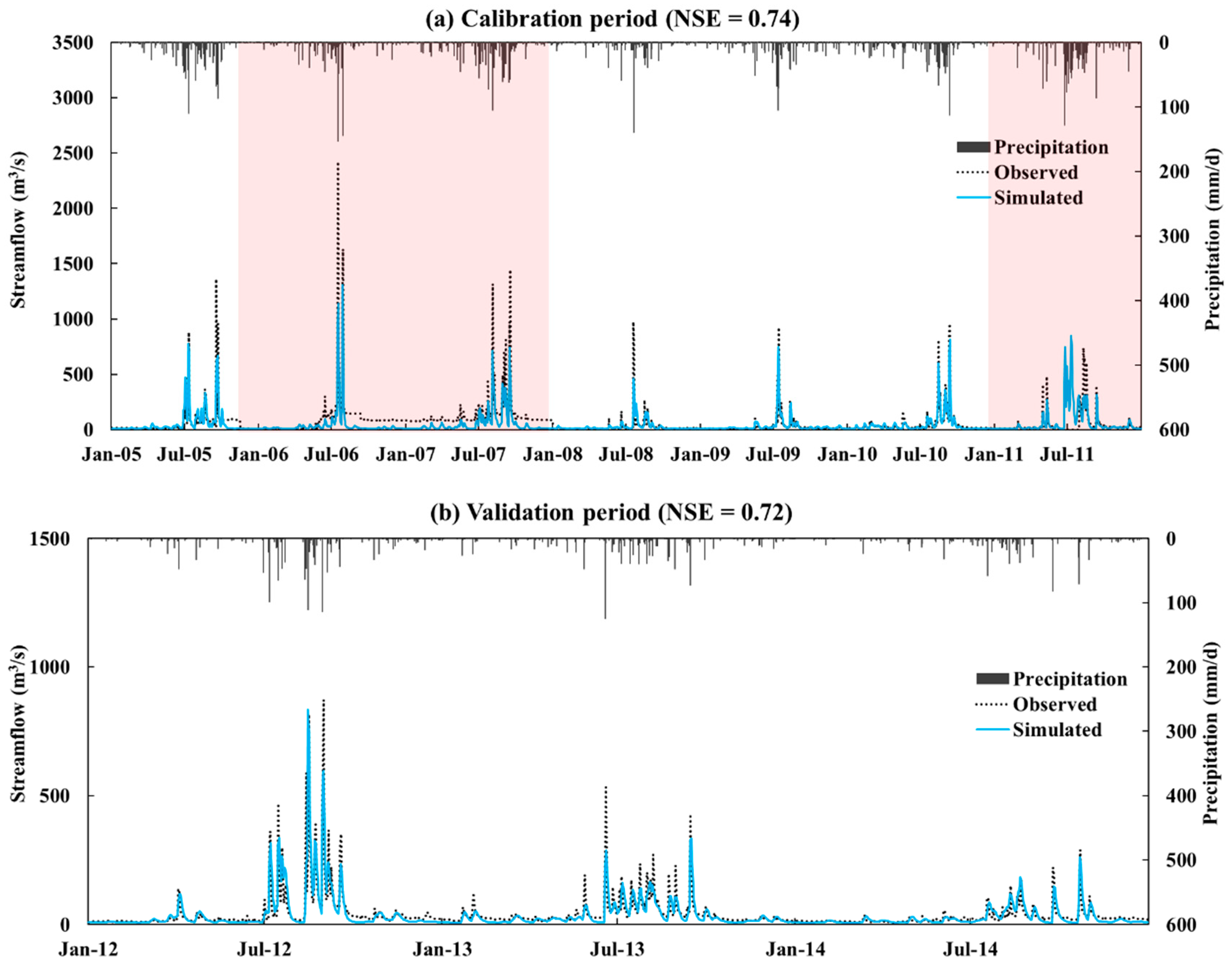
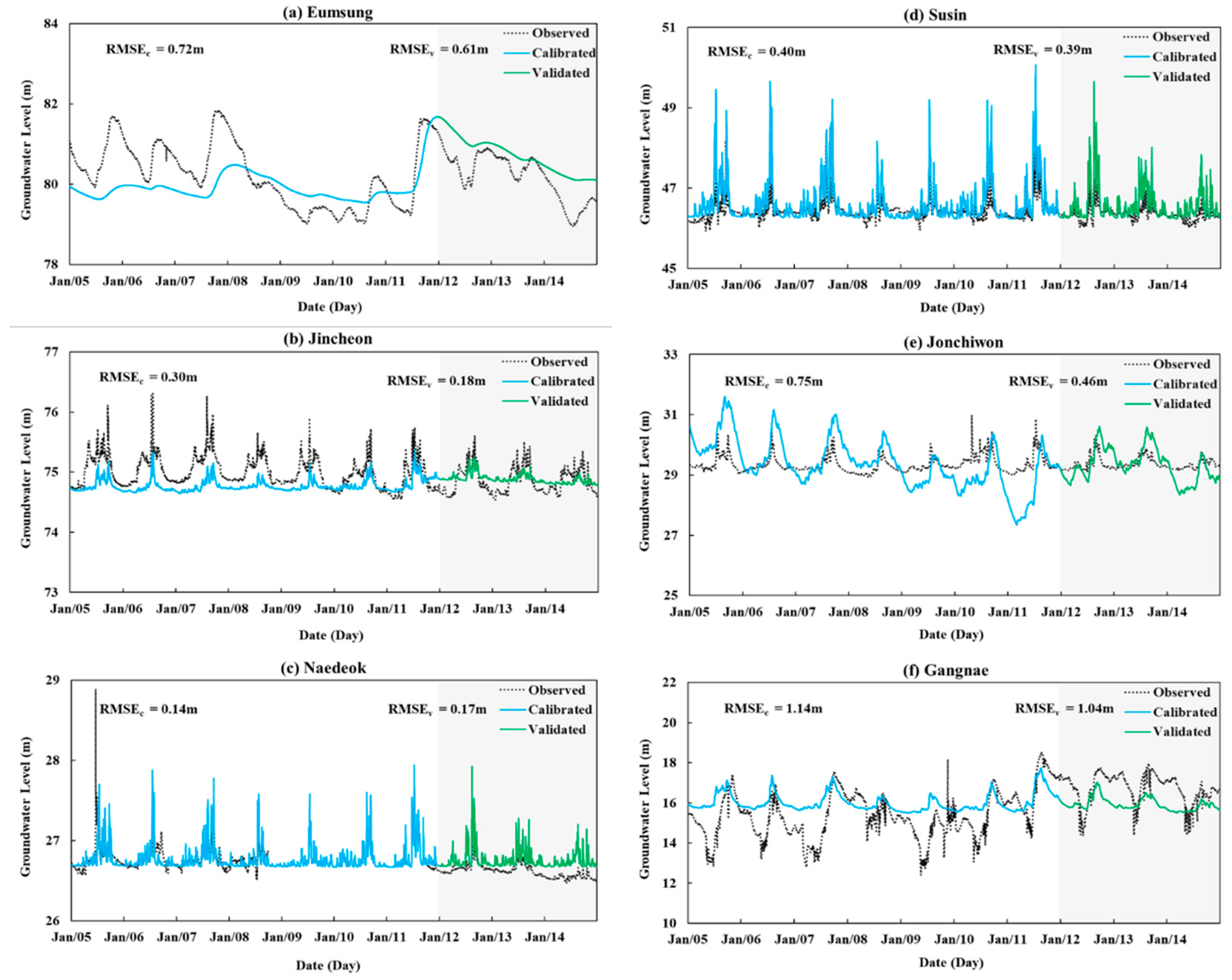
4.1. Model Performance

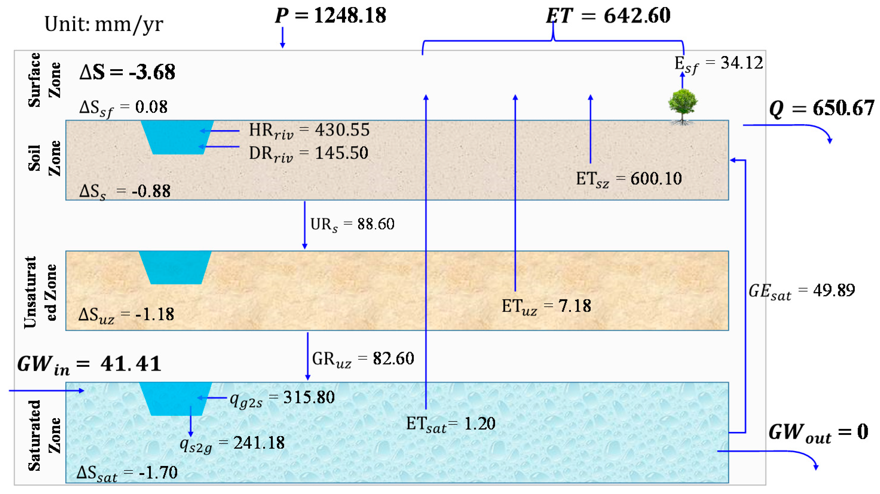
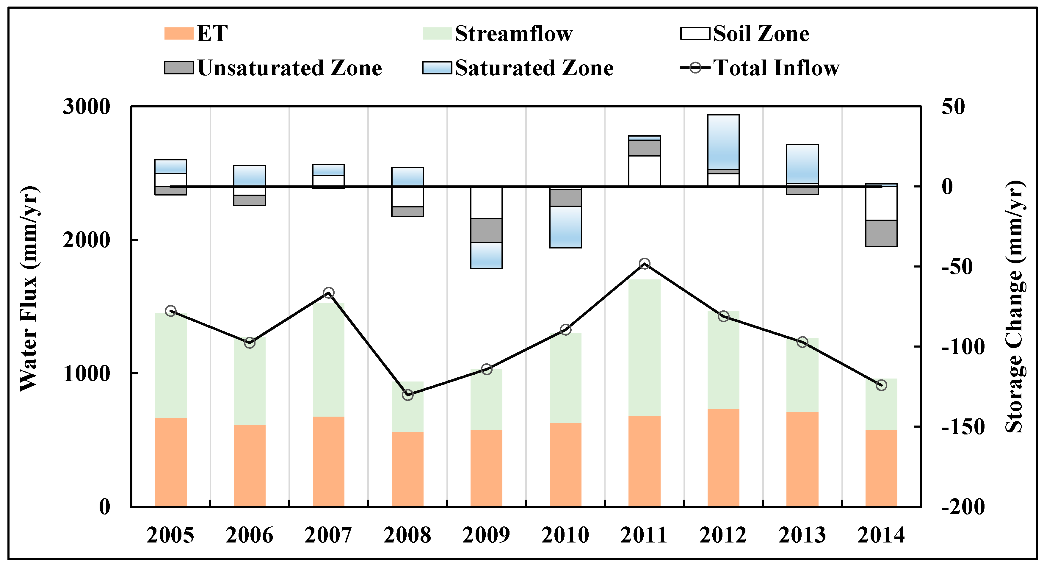
The GSFLOW model of the Miho catchment was run at a daily time step from 1 January 2004 to 31 December 2014. The first year (i.e., 2004) was run as a warm up period to establish the initial soil zone and unsaturated zone storages [44]. Thus, the first year was excluded from the calibration. The streamflow and groundwater head calibration period was from 1 January 2005 to 31 December 2011 (seven years in total), and the remaining three years were treated as the validation period.

Figure 4 shows comparisons of the simulated and observed streamflows during the calibration and validation periods at the Hapgang gauging station. The observed streamflow in 2006, 2007 and 2011, as indicated by the shaded areas of the hydrograph in Figure 4a, indicates a problem in the low and high flow regimes due to rating curve errors. After eliminating these incorrect observed streamflow values, the calculated NSE equals 0.74 and 0.72, the ${\mathrm{R}}^2$ equals 0.73 and 0.74, the AARE equals 0.43 and 0.39, and the $T{S}_{25}$ equals 0.72 and 0.83 for the calibration and validation periods, respectively. The goodness of fit metrics indicate that the model accurately reproduced the overall observed hydrographs on a daily time scale. However, discrepancies in some of the peak events between the calibration and validation periods were also found. One explanation for these discrepancies is that the precipitation interpolated from the limited rainfall stations was not accurate, especially during storm periods. Another explanation is that the rainfall during storms occur locally.

To investigate the model performance of the groundwater flow simulation, the simulated and observed groundwater heads during the calibration and validation periods were compared at six national observation wells, as demonstrated in Figure 1b. Three distinct patterns of groundwater head fluctuation could be identified based on the observations from these observation wells in Figure 5. First, the groundwater head fluctuation was greatly affected by variations in the streamflow, as indicated by the Nadeok and Susin wells, which were very close to rivers. Second, the fluctuation of groundwater head had a slow response to streamflow, as indicated by the Jincheon, Jonchiwon, and Gangnae wells, which were located farther from rivers in Figure 1b. Last, the groundwater head fluctuation exhibited a considerably smaller variation than those of the previous two patterns, as indicated by the Eumsung well, which was in a mountainous area. The first two fluctuation patterns were mainly controlled by stream-aquifer interactions. The third pattern was dominated by climate variation during calibration and validation period. Overall, the calibrated model captured these three patterns very accurately. However, it is still difficult to precisely reproduce the groundwater fluctuation in mountainous areas, as indicated by the simulated groundwater heads at the Jincheon and Eumsung monitoring wells, in the model. Nevertheless, the calibrated model still captured the long-term trend of the groundwater heads in these areas.

4.2. Water Balance

The water balance analysis of the Miho catchment was calculated by water balance equations in Section 3.4. The schematic diagram in Figure 6 illustrates the annual water balance of the whole model domain (averaged over 2005–2014) and the fluxes among the vertical conceptual zones. The

Table 2. List of symbols used in the schematic diagram in Figure 6.

Variables	Description	Variables	Description
P	Precipitation	ETuz	Evapotranspiration from unsaturated zone
∆S	Total storage change	GEsat	Groundwater exfiltration
∆Ss	Storage change in soil zone	GRuz	Recharge to saturated zone
∆Ssat	Storage change in saturated zone	GWin	Groundwater inflow
∆Ssf	Storage change on surface	GWout	Groundwater outflow
∆Suz	Storage change in unsaturated zone	HRriv	Surface runoff
DRriv	Soil zone inter flow	Q	Total runoff of the catchment
Esf	Evapotranspiration from surface	qg2s	Goundwater discharge to stream
ET	Total Evapotranspiration	qs2g	Stream leakage to GW
ETsat	Evapotranspiration from saturated zone	URs	Percolation from soil zone
ETsz	Evapotranspiration from soil zone

describes the variables in the Figure 6. The fluxes shown in Figure 6 are area-averaged values over the entire study area. For the whole domain, the inputs of the system are precipitation ($P=1248.18 \mathrm{mm}/\mathrm{yr}$) and groundwater inflow (${\mathrm{GW}}_{in}=41.41 \mathrm{mm}/\mathrm{yr}$), the outputs are evapotranspiration ($ET=642.60 \mathrm{mm}/\mathrm{yr}$) and streamflow ($Q=650.67 \mathrm{mm}/\mathrm{yr}$), and the total storage change is $\Delta \mathrm{S}=-3.68 \mathrm{mm}/\mathrm{yr}$. In this study, it was assumed that ${\mathrm{GW}}_{out}$ equals zero. Because the study area is a typical humid catchment, $ET$ equals 51.5% of $P$, and $Q$ equals 52.1% of $P$. The ET in Equation (8) has one surface component, ${\mathrm{E}}_{sf}=34.12 \mathrm{mm}/\mathrm{yr}$ (5.3% of ET and 2.7% of P), and three subsurface components, ${\mathrm{ET}}_{sz}=600.1 \mathrm{mm}/\mathrm{yr}$ (93.4% of ET and 48.1% of P), ${\mathrm{ET}}_{uz}=7.18 \mathrm{mm}/\mathrm{yr}$ (1.1% of ET and 0.6% of P) and ${\mathrm{ET}}_{sat}=1.20 \mathrm{mm}/\mathrm{yr}$ (0.2% of ET and 0.1% of P). The streamflow $Q$ in Equation (9) consists of the surface runoff ${\mathrm{HR}}_{riv}=430.5 \mathrm{mm}/\mathrm{yr}$ (66.2% of $\mathrm{Q}$), soil zone interflow ${\mathrm{DR}}_{riv}=145.5 \mathrm{mm}/\mathrm{yr}$ (22.4% of $\mathrm{Q}$), and net groundwater discharge to the streams ${\mathrm{q}}_{g2s}-{\mathrm{q}}_{s2g}74.62 \mathrm{mm}/\mathrm{yr}$ (11.4% of $\mathrm{Q}$). The negative $\Delta \mathrm{S}$ is mainly due to the depletion of the groundwater storage (46.2% of $\Delta \mathrm{S}$) and drying of the unsaturated zone (32.1% of $\Delta \mathrm{S}$) and soil zone (23.9% of $\Delta \mathrm{S}$), while the storage change in the surface was negligible.

The water balance of the surface and soil zones includes two inputs, $\mathrm{P}$ and groundwater exfiltration ${\mathrm{GE}}_{sat}$ (48.89 mm/yr); and five outputs, ${\mathrm{E}}_{sf}$ (2.7% of $\mathrm{P}$), ${\mathrm{ET}}_{sz}$ (48.1% of $\mathrm{P}$), surface runoff ${\mathrm{HR}}_{riv}$ (34.5% of $\mathrm{P}$), soil zone interflow ${\mathrm{DR}}_{riv}$ (11.7% of P), and percolation to the unsaturated zone ${\mathrm{UR}}_s$ (7.0% of $\mathrm{P}$). The water balance of the unsaturated zone includes only one input, percolation from the soil zone ${\mathrm{UR}}_s$, and two outputs, recharge to the saturated zone ${\mathrm{GR}}_{uz}$ (82.60 mm/yr) and evapotranspiration from the unsaturated zone ${\mathrm{ET}}_{uz}$ (7.18 mm/yr). It can be seen that most of ${\mathrm{UR}}_s$ is converted to ${\mathrm{GR}}_{uz}$. The saturated zone water balance includes three inputs, ${\mathrm{GR}}_{uz}$ (82.60 mm/yr), ${\mathrm{GW}}_{in}$ (41.41 mm/yr) and ${\mathrm{q}}_{s2g}$ (241.80 mm/yr), and four outputs, ${\mathrm{ET}}_{sat}$ (1.20 mm/yr), ${\mathrm{q}}_{g2s}$ (315.80 mm/yr), ${\mathrm{GE}}_{sat}$ (241.80 mm/yr) and ${\mathrm{GW}}_{out}$ (0 mm/yr). The stream leakage contributes 66% of the total groundwater recharge (365.19 mm/yr). As illustrated in Figure 6, the surface water and groundwater interactions in the Miho catchment are significant and play a critical role in the water cycle.

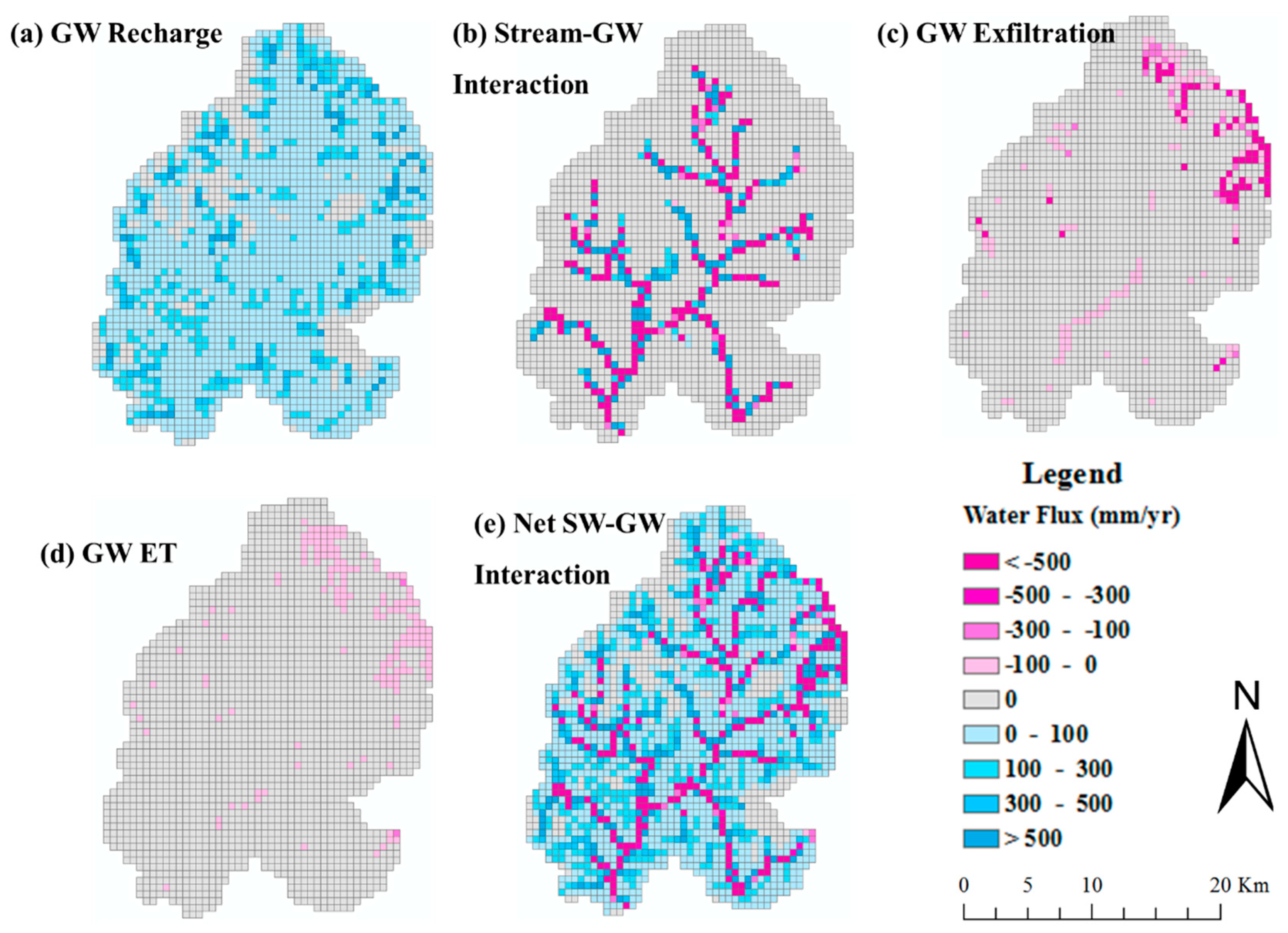
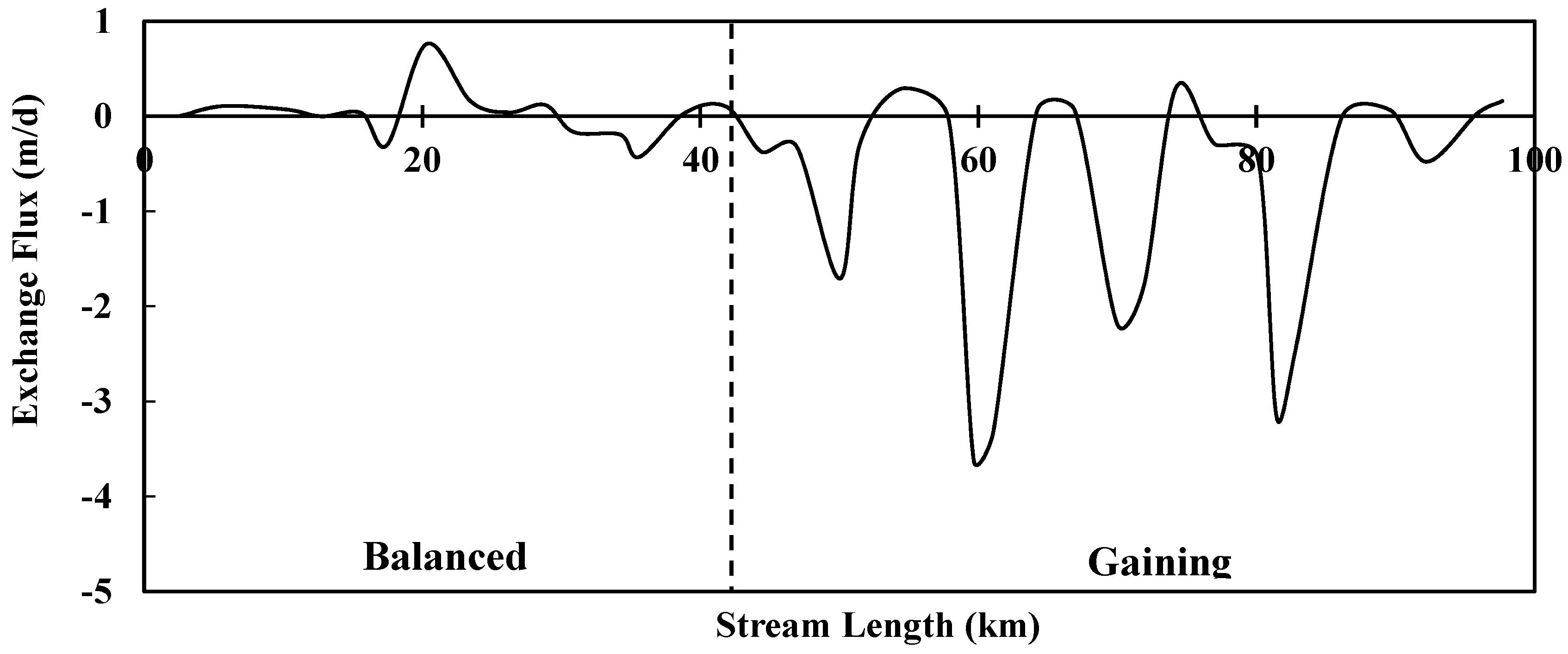
4.3. Spatial Variability in the SW–GW Interactions

The spatial distribution of the annual averaged SW–GW interaction fluxes (averaged over 2005–2014) are presented in Figure 7. Positive values indicate that the surface water recharges to the groundwater, while negative values indicate groundwater exfiltration to the soil zone or streams. The fluxes in Figure 7 consist of four components, GW recharge (${\mathrm{GR}}_{uz}$), stream GW interaction (${\mathrm{q}}_{s2g}$ and ${\mathrm{q}}_{g2s}$), GW exfiltration (${\mathrm{GE}}_{sat}$) and GW ET (${\mathrm{ET}}_{sat}$). These four components are presented in Figure 7a–d, respectively. Figure 7e presents the net flux ${\mathrm{SG}}_{net}$, which is the sum of ${\mathrm{GR}}_{uz}$, ${\mathrm{q}}_{s2g}, {\mathrm{q}}_{g2s}, {\mathrm{GE}}_{sat}$, and ${\mathrm{ET}}_{sat}$. Significant spatial variability in the SW–GW interaction fluxes could be identified in Figure 7.

The spatial variability in ${\mathrm{GR}}_{uz}$ (Figure 7a) ranged from nearly 0 mm/yr in the mountain areas to 300 mm/yr in the flat areas and along stream valleys. This variability may be attributed to hilly topography with complicated drainage patterns and spatially variable land uses. The most active SW–GW interactions occurred along the streams. Figure 7b shows the spatial pattern of the stream–aquifer interaction; most of stream leakage occurred in the upper streams with relatively steep streambed slopes. In lower streams, the aquifer gained water from the streams. Figure 8 further demonstrates the spatial pattern of the SW–GW exchange flux (i.e., volume of water per unit area of streambed per unit time) along the main stream, and two distinct exchange patterns are clearly identified. In the upper mainstream with a length of 47 km, the stream leakages are roughly equal to the groundwater discharge. In the lower mainstream with a length of 50 km, the stream gains water from the aquifer since the groundwater head is higher than the stream water level. The gained water is approximately 0.145 billion m³ per year.

Figure 7c shows the spatial variability in ${\mathrm{GE}}_{sat}$. ${\mathrm{GE}}_{sat}$ was the largest in the northeast area, where the water table was very shallow. ${\mathrm{GE}}_{sat}$ was also considerably large in the lower reaches of the main stream. In the other areas of the catchment, the water table was relatively deep; therefore, ${\mathrm{GE}}_{sat}$ was negligible. ${\mathrm{ET}}_{sat}$ (Figure 7d) also exhibited a spatial variability pattern controlled by the depth to the water table. This similarity is likely why the ${\mathrm{ET}}_{sat}$ pattern was similar to the ${\mathrm{GE}}_{sat}$ pattern, which were both characterized by high groundwater discharge rates along the streams and in areas with a shallow water table. The map of ${\mathrm{SG}}_{net}$ (Figure 7e) combines all recharge and discharge components, highlighting recharge areas with ${\mathrm{SG}}_{net}>0$ and discharge areas with ${\mathrm{SG}}_{net}<0$. ${\mathrm{SG}}_{net}$ was positive in most of the study area but negative along the streams.

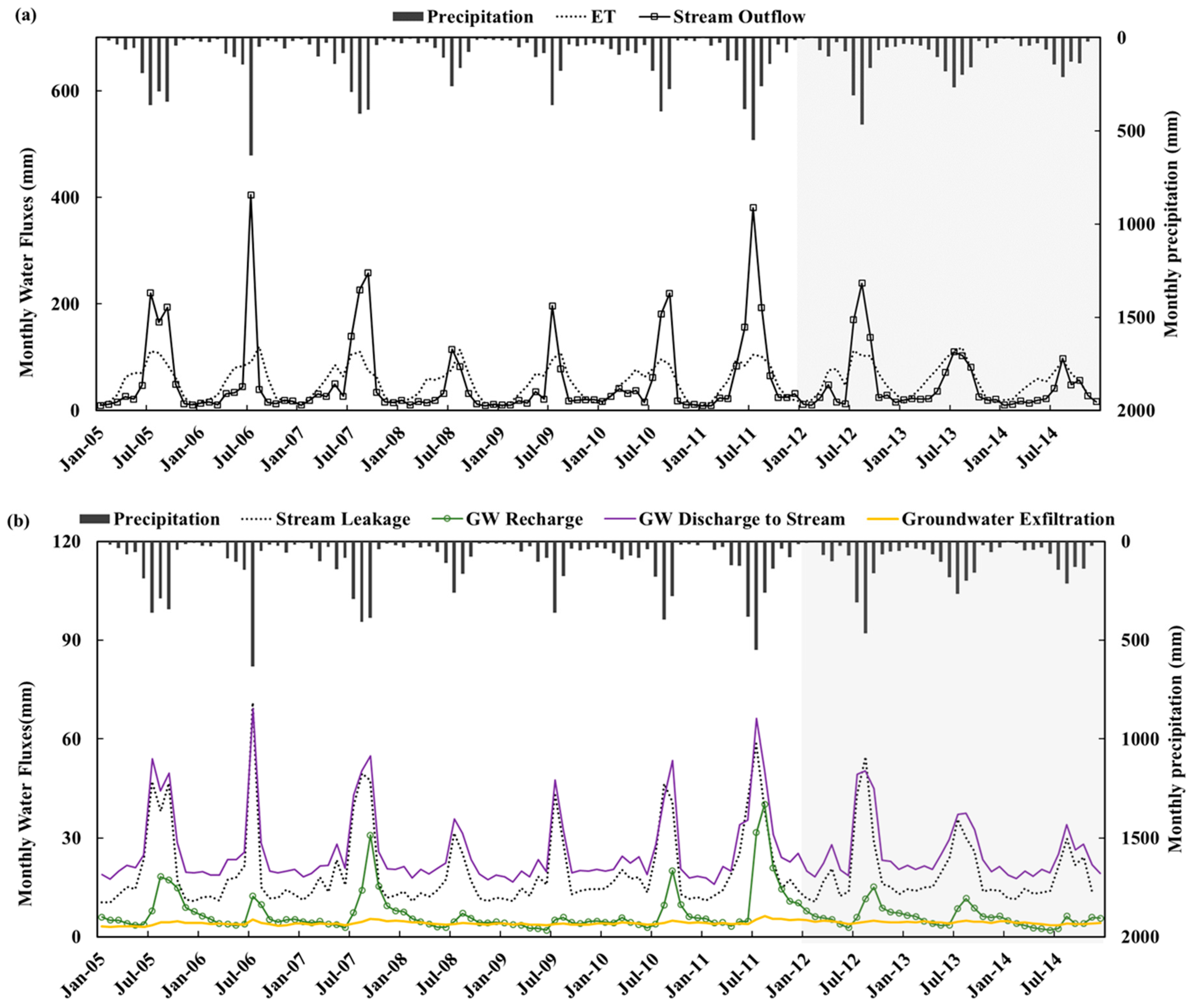
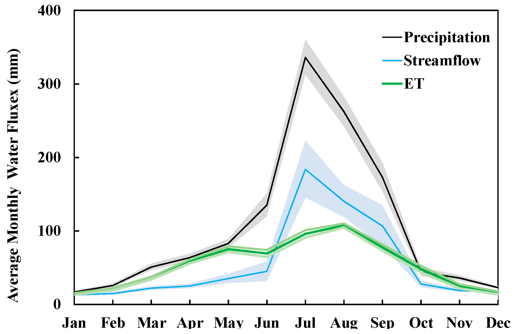
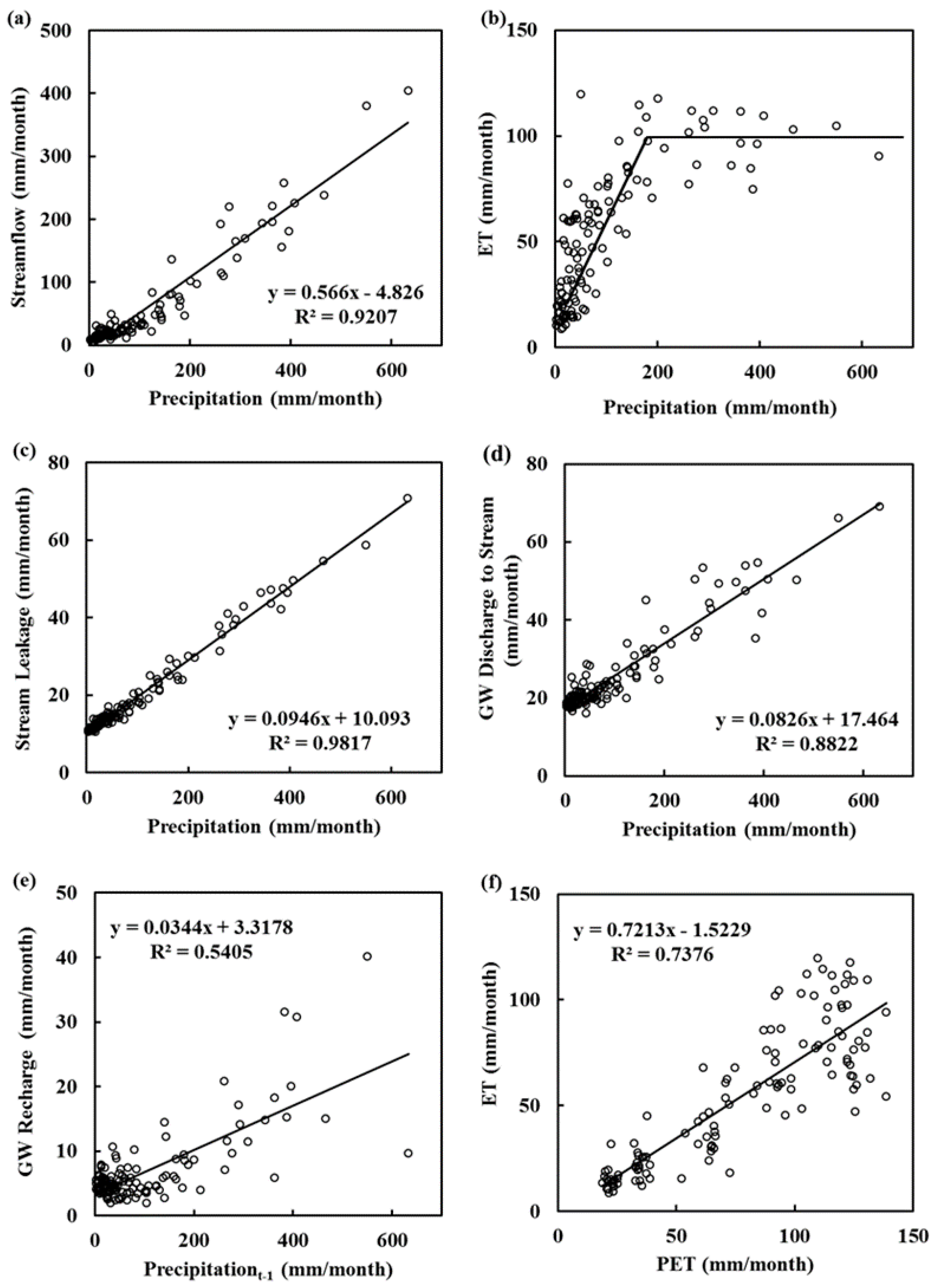
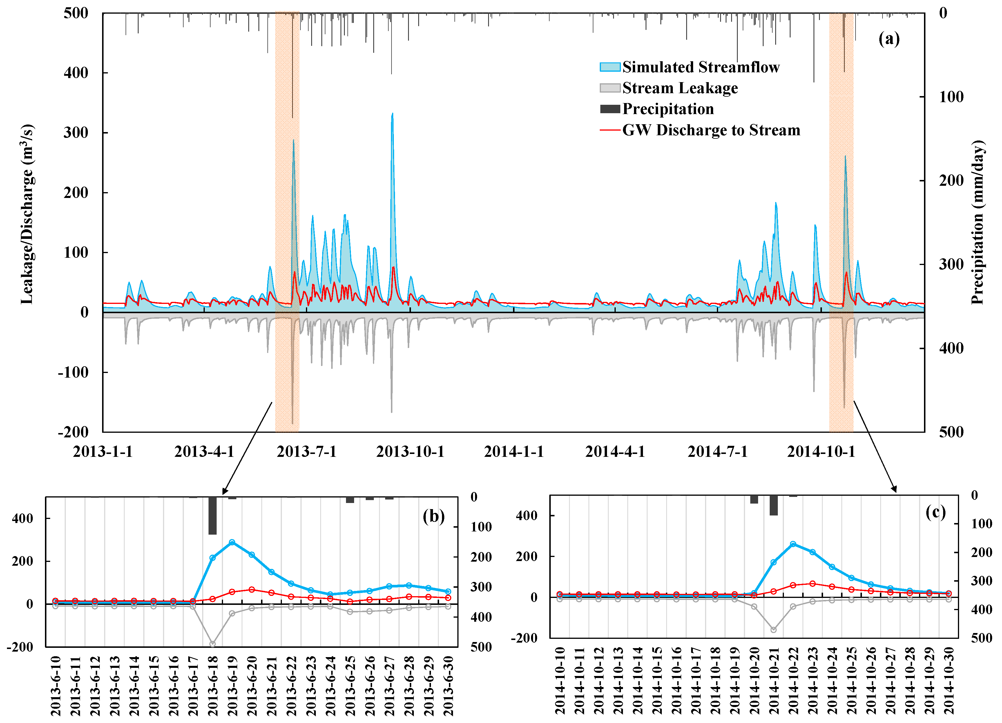
4.4. Temporal Variability in the Water Fluxes

Figure 9 presents the monthly variability in the major water balance components over the 10-year simulation period (2005–2014). Figure 9a reveals a clear seasonality with high precipitation ($P$) and streamflow ($\mathrm{Q}$) in the summer/autumn and a period of decreased flows in the winter/spring. The amplitude of this seasonality was variable with pronounced wet (2005–2007 and 2011–2012) and dry (2008–2010 and 2013–2014) periods. Figure 10 further illustrates the seasonal pattern of monthly $P$, $\mathrm{Q}$ and $ET$. $P$ was, on average, greatest in July (311–360 mm) and lowest in January (14–18 mm). $\mathrm{Q}$ was also highest in July (144–222 mm). $\mathrm{Q}$ reached a minimum in January (11–14 mm). However, monthly ET was relatively consistent from year to year. $ET$ reached a maximum in August (110–118 mm) and was at a minimum in January (13–15 mm). The temporal variability in the water fluxes related to the SW–GW interactions are presented in Figure 9b. Both the stream leakage to the groundwater (${\mathrm{q}}_{s2g}$) and groundwater discharge (${\mathrm{q}}_{g2s}$) to the streams exhibited a strong temporal variability, while the groundwater recharge (${\mathrm{GR}}_{uz}$) showed moderate temporal variability. However, the groundwater exfiltration (${\mathrm{GE}}_{sat}$) was approximately constant.

The temporal variability in the water fluxes was further investigated through correlation analysis. The correlations between $P$ and $Q$, $ET$, ${\mathrm{q}}_{s2g}$, ${\mathrm{q}}_{g2s}$ and ${\mathrm{GR}}_{uz}$ are depicted in Figure 11a–e, respectively. A distinct difference in the temporal variability between $\mathrm{Q}$ and $\mathrm{ET}$ was identified by comparing Figure 11a,b. The strong linear relationship between $\mathrm{P}$ and $\mathrm{Q}$ (${\mathrm{R}}^2=0.92$) suggests that the temporal variability in $\mathrm{Q}$ was dominated by $\mathrm{P}$. However, the temporal variability in $ET$ was likely controlled by the potential ET (PET) rather than by $\mathrm{P}$. As shown in Figure 11b, for monthly $P$ values less than 180 mm, $ET$ was linearly correlated with $P$; but for monthly $P$ values greater than 180 mm, ET was consistently limited by the increase in $P$. This threshold likely corresponds to the energy-constrained maximum evaporative capacity of the Miho catchment. Assuming that soil moisture is adequate, evapotranspiration is dependent primarily on the energy available to vaporize the water. The energy equals to net radiation minus soil heat flux. Therefore, the ET process in the Miho catchment is generally energy-limited rather than water-limited. This energy-limitation effect can also be identified in Figure 11f.

The temporal variability in the monthly ${\mathrm{q}}_{s2g}$ and ${\mathrm{q}}_{g2s}$ tends to be influenced by the monthly $P$. The R² values between $P$ and ${\mathrm{q}}_{s2g}$ and between $P$ and ${\mathrm{q}}_{g2s}$ were equal to 0.98 (Figure 11c) and 0.88 (Figure 11d), respectively. Through a series of lag-correlation analyses, we found that the monthly ${\mathrm{GR}}_{uz}$ was influenced by precipitation during the previous month (donated as Precipitation _t-1 in Figure 11e). This one-month lag between ${\mathrm{GR}}_{uz}$ and $P$ was likely caused by the damping effect of the unsaturated zone. The groundwater exfiltration (${\mathrm{GE}}_{sat}$) indicated a weaker dependence on the seasonal climatic variability (Figure 9b). The relationship between $P$ and ${\mathrm{GE}}_{sat}$ is not presented in this study.

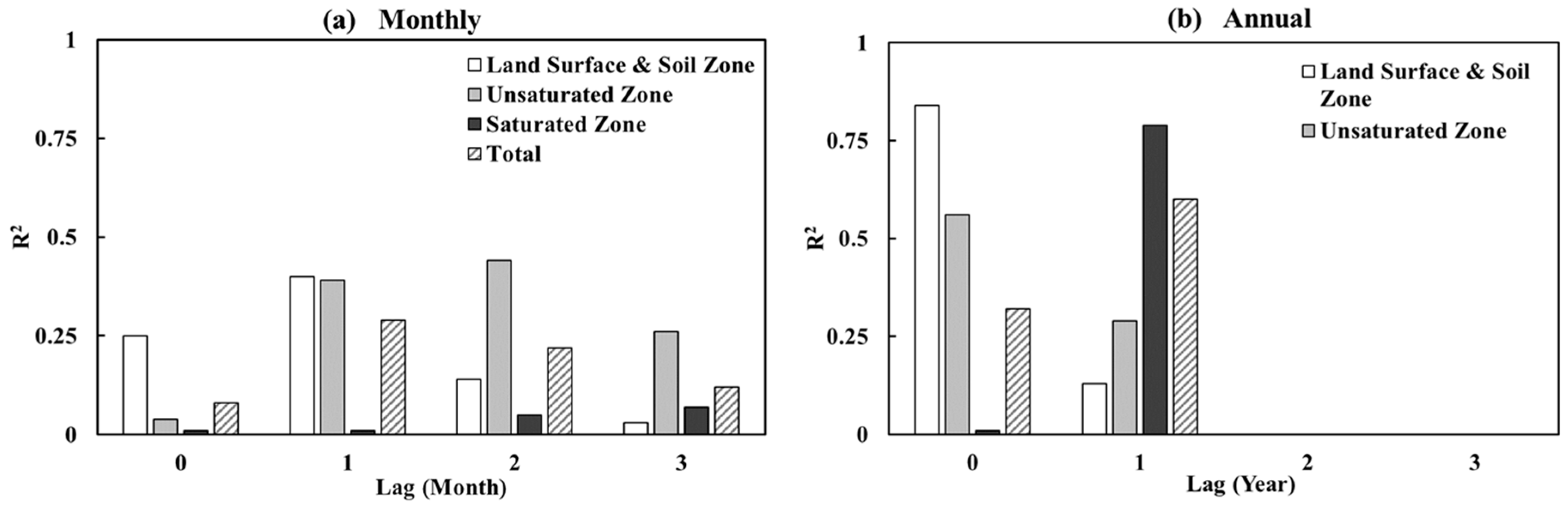
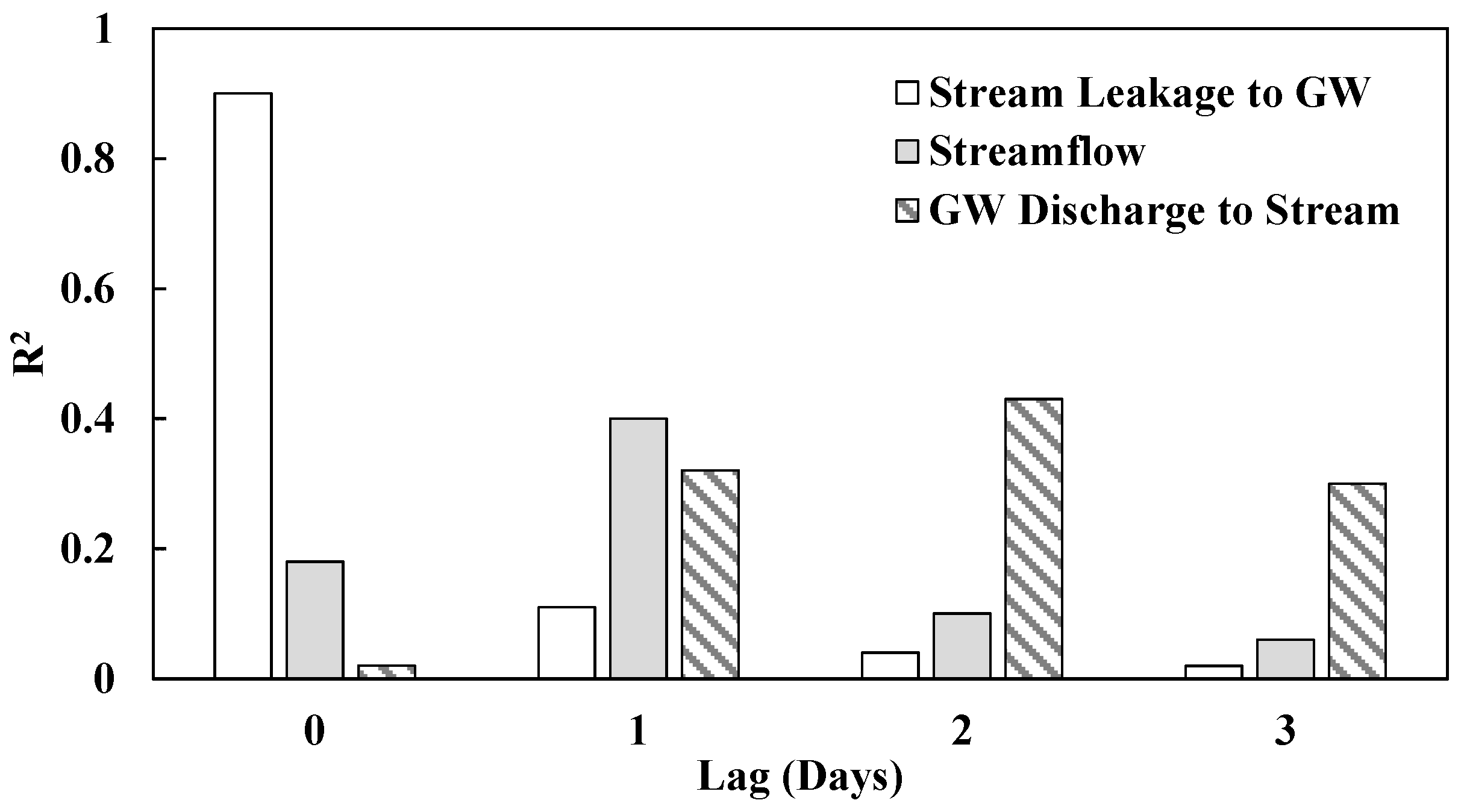
4.5. Influence of the Temporal Damping Effects on the Hydrological Cycle

The impacts of the damping effects on the hydrological cycle can be found at different temporal and spatial scales. The changes in the monthly storage at the catchment scale were calculated in the following zones: (1) surface and soil zone; (2) unsaturated zone; and (3), saturated zone (Figure 12). Note that storage change does not refer to an actual storage value but rather represents the storage relative to an arbitrary storage starting value of 0 at the beginning of the time series. Likewise, negative storage values mean that the storage was below the initial storage state. It can be seen that the temporal variability in the storage change in different zones are significantly different. These different patterns may result from temporal damping effects of the hydrological system in the study area. The highly variable precipitation may rapidly infiltrate into the soil zone, resulting in a quick response of the soil moisture. As a result, the storage change in the soil zone ($\Delta {\mathrm{S}}_{sz}$) had a large temporal variability. When the precipitation percolated through the unsaturated zone, the infiltration pulses were damped due to the lower permeability of the unsaturated zone. This damping effect was also reflected in a one-month lag between $P$ and ${\mathrm{GR}}_{uz}$ (Figure 11e). The percolations to deeper groundwater were further damped by the saturated zone, resulting in the smallest temporal variability in the storage change in the saturated zone ($\Delta {\mathrm{S}}_{sat}$). Overall, the hydrological system acts as a low-pass filter that dampens the high-frequency fluctuations of the input signal. The longer the input hydrological signal (i.e., $P$) propagates through the system, the smoother the responses are (i.e., $\Delta {\mathrm{S}}_{sat}$). Due to the temporal damping effect, the Miho catchment exhibited pronounced time dependencies of the hydrologic responses to precipitation on monthly and annual time scales.

To reveal the impact of the temporal damping effect on the storage change, lag-correlation analyses between $P$ and $\Delta {\mathrm{S}}_{sz}$, $\Delta {\mathrm{S}}_{uz}$, $\Delta {\mathrm{S}}_{sat}$ and $\Delta \mathrm{S}$ were calculated on monthly and annual time scales. On a monthly time scale (Figure 13a), it can be seen that the correlation between $P$ and $\Delta {\mathrm{S}}_s$ was strongest at a lag of one month, meaning that $P$ had a stronger influence on $\Delta {\mathrm{S}}_{sz}$ during the previous month than during the same month. The lag correlation became insignificant after two months. In the unsaturated zone, the highest correlation was at a lag of two months. The lag correlation became insignificant after three months, suggesting a longer temporal damping effect. In the saturated zone, the correlation was insignificant at lags of up to six months, meaning that its damping effect would occur at time scales longer than monthly. The lag correlation for the total storage followed a pattern similar to that in the soil zone, indicating that the soil zone played a dominant role in damping the precipitation on a monthly time scale.

On the annual time scale (Figure 13b), at zero lag (annual precipitation correlated with the storage during the same year), the correlations were significant for the soil zone and unsaturated zone but insignificant and weak for the saturated zone and whole system. However, at a lag of one year (annual storage correlated with the precipitation during the previous year), significant positive correlations emerged for the saturated zone and whole system, suggesting that the saturated zone plays a dominant role in damping precipitation at the annual scale.

The damping effect can be further analyzed by the annual variability in the hydrological system of inputs/outputs and storage changes, which are demonstrated in Figure 14. The total inflow ${\mathrm{F}}_{in}$ is the sum of $P$ and ${\mathrm{GW}}_{in}$. In the surface domain, the fluctuation of the annual $Q$ coincided with ${\mathrm{F}}_{in}$. The annual $ET$ was relatively constant throughout the years. In the subsurface domain, the annual storage dynamics were greatly affected by the damping effects. The storage in the soil zone and unsaturated zone were primarily determined by the precipitation in the same year. The soil zone and unsaturated zone tended to gain water in wetter years and lose water in drier years. However, this tendency was complicated by the storage state during the previous year. The storage in the saturated zone mostly depended on the precipitation during the previous year. This one-year lag between $P$ and $\Delta {\mathrm{S}}_{sat}$ is clearly illustrated in Figure 14, especially from 2008 to 2012. In 2008, the Miho catchment experienced serious drought; during this time, the precipitation was only 797 mm, which was 64% of the average annual precipitation (1248 mm). Due to the geological characteristics of the Miho catchment, the storage changes in the soil zone and unsaturated zone decreased, indicating a quick response to the drought. However, the storage change in the saturated zone still increased because of the earlier wet period during 2007. In the following three years, the precipitation continually increased and reached a maximum in 2011 (1781 mm). Correspondingly, $\Delta {\mathrm{S}}_s$ and $\Delta {\mathrm{S}}_{uz}$ gradually recovered and reached maximums in 2011. The recovery of $\Delta {\mathrm{S}}_{sat}$ showed a one-year lag behind $\Delta {\mathrm{S}}_s$ and $\Delta {\mathrm{S}}_{uz}$.

At smaller spatial and time scales, the temporal damping effect was also found in the stream-aquifer interaction. To explore this effect, lag correlations between $P$ and streamflow ($\mathrm{Q}$), stream leakage to the groundwater ${\mathrm{q}}_{s2g}$ and groundwater discharge to the streams ${\mathrm{q}}_{g2s}$ were calculated on a daily time scale. The values of ${\mathrm{q}}_{s2g}$ and ${\mathrm{q}}_{g2s}$ were calculated by considering all the stream reaches. The strongest correlations between $P$ and ${\mathrm{q}}_{s2g}$, $\mathrm{Q}$ and ${\mathrm{q}}_{g2s}$ were found at a lag of zero days, one day and two days, respectively (Figure 15). During a rainstorm event, rainfall was quickly converted to flood runoff, usually in less than one day. The flash flood runoff tended to develop a flood wave that traveled downstream. The flood wave caused a rapid rise in the stream head, which in turn resulted in an abrupt stream leakage if the stream head was significantly higher than the groundwater head in the channel. The time that it took the flood runoff to travel from the headwater to the outlet was approximately one day; thus, the daily $\mathrm{Q}$ shows a lag of one day behind the daily $P$. Because the flood wave celerity is faster than the flow velocity, the time lag between $P$ and ${\mathrm{q}}_{s2g}$ is smaller than that between $P$ and $\mathrm{Q}$. The stream head receded gradually after the crest of the last flood wave arrived. The leakage that percolated through the stream bed was damped by the aquifer. When the damped leakage reached the groundwater table, the groundwater head would abruptly increase and exceed the stream head, resulting in an abrupt groundwater discharge to the stream. This damping effect likely led to a lag of approximately 2 days between the daily $P$ and daily ${\mathrm{q}}_{s2g}$.

To better understand the role of stream–groundwater interaction in hydrograph recession, the daily time series of the simulated streamflow $\mathrm{Q}$ at the catchment outlet, ${\mathrm{q}}_{s2g}$ and ${\mathrm{q}}_{g2s}$ from 2013 to 2014 is illustrated in Figure 16. The negative values indicate stream recharges to the groundwater. As shown in Figure 16a, the storm precipitations were always followed by prompt changes in ${\mathrm{q}}_{s2g}$. In contrast, $\mathrm{Q}$ and ${\mathrm{q}}_{g2s}$ lagged behind $\mathrm{P}$ by one day and two days, respectively. This time lag pattern is clearly illustrated by the two flood events shown in Figure 16b,c.

4.6. Implications for Water Resources Management

Natural hazards such as flooding and drought increasingly result in significant damages. According to the latest Intergovernmental Panel on Climate Change (IPCC) report, drought frequencies and intensities may increase in the coming decades [45]. Meanwhile, the frequency and intensity of heavy precipitation events may also increase. Catchment responses to climate changes are largely a function of storage, which acts as a buffer between the water inputs and streamflow response [17]. At the Miho catchment, variability in the capacity to buffer the earlier precipitation can be observed across the entire catchment, from small to large scales. The streamflow exhibited one-day lag behind the precipitation, and the aquifers had one-year lags behind precipitation. These lags are of great importance for flood control and drought management. At the catchment scale, our results suggest that it can take one year after a drought period to refill the storage in an aquifer system. We can even forecast the storage change in the aquifer in the next year by considering the precipitation in the current year. These implications are of critical importance to developing a management regime that accounts for both the surface and subsurface water resources. The integrated modeling approach introduced in this study can offer valuable help.

5. Conclusions

In this study, we presented a systematic modeling study of complex hydrological processes in a typical humid area using an integrated SW–GW modeling approach. We also investigated the spatial variability in the surface water-groundwater interactions, temporal variability in the water fluxes, and influences of the temporal damping effects on the hydrological cycle by evaluating 10 years of observational data and modeling results. The major findings of this study are summarized below.

First, complex dynamics of surface water-groundwater interactions in humid areas requires that all the important hydrologic processes be simulated simultaneously in an integrated framework. GSFLOW applied in this study meets this requirement. Its ability to simulating whole hydrological cycle enables to reveal complicated non-linear processes such as surface runoff, groundwater recharge and exfiltration.

Second, the simulated results for the 10-year period indicate that the SW–GW interactions in the study area are significant and mainly occur within the streams. The SW–GW exchange in stream has notable spatial and temporal variations. The temporal variability in the streamflow, stream-groundwater interactions and groundwater recharge are mainly dominated by precipitation, while the temporal variability in the ET is controlled by the energy (net radiation minus soil heat flux) conditions. Third, the damping effects can influence the hydrological cycle across different temporal scales and spatial scales. Overall, the SW–GW system acts as a low-pass filter and dampens the high-frequency fluctuations of the input signal (precipitation). The longer the input hydrological signal propagates through the system, the smoother the responses are.

Finally, variability in the capacity to buffer earlier precipitation is observed at small spatial scales, such as streams, and larger spatial scales, such as the whole catchment. This variability could affect the water balance at larger spatial scales and affect the hydrography recession at smaller spatial scales. Understanding these buffering capabilities is of critical importance for the development of effective flood and drought management strategies.

It is worthwhile pointing out that several limitations are associated with study. First, the model was calibrated using a trial-and-error approach. This calibrating approach is not efficient when many parameters need to be calibrated and they affect each other. Second, several assumptions were made during the modeling due to limitation of data availability, such as the time-invariant groundwater inflow conditions and rectangle river cross sections. These assumptions may hamper accuracy of modeling results. In future studies, we will improve model calibration by employ optimization algorithm. The uncertainties induced by the assumptions will be investigated.

References

1. Winter, T.; Harvey, J.; Franke, O.; Alley, W. Natural Processes of Ground-Water and Surface–Water Interaction; Ground Water and Surface Water: A Single Resource; US Geological Survey Circular: Denver, CO, USA, 1998; Volume 1139, pp. 2–50.
2. Seibert, J.; Bishop, K.; Nyberg, L.; Rodhe, A. Water storage in a till catchment. I: Distributed modelling and relationship to runoff. Hydrol. Processes 2011, 25, 3937–3949. [Google Scholar] [CrossRef]
3. Spanoudaki, K.; Stamou, A.I.; Nanou-Giannarou, A. Development and verification of a 3-D integrated surface water–groundwater model. J. Hydrol. 2009, 375, 410–427. [Google Scholar] [CrossRef]
4. Zhang, Q.; Li, L. Development and application of an integrated surface runoff and groundwater flow model for a catchment of Lake Taihu watershed, China. Quat. Int. 2009, 208, 102–108. [Google Scholar] [CrossRef]
5. VanderKwaak, J.E. Numerical Simulation of Flow and Chemical Transport in Integrated Surface-subsurface Hydrologic Systems. Ph.D. Thesis, University of Waterloo, Waterloo, ON, Canada, 1999. [Google Scholar]
6. Abbott, M.B.; Bathurst, J.C.; Cunge, J.A.; O’Connell, P.E.; Rasmussen, J. An introduction to the European Hydrological System—Systeme Hydrologique Europeen, “SHE”, 2: Structure of a physically-based, distributed modelling system. J. Hydrol. 1986, 87, 61–77. [Google Scholar] [CrossRef]
7. Graham, N.; Refsgaard, A. MIKE SHE: A distributed, physically based modeling system for surface water/groundwater interactions. In Proceedings of the MODLFOW 2001 and Other Modeling Odysseys, Golden, CO, USA, 2001. [Google Scholar]
8. Brunner, P.; Simmons, C.T. HydroGeoSphere: A fully integrated, physically based hydrological model. Groundwater 2012, 50, 170–176. [Google Scholar] [CrossRef]
9. Maxwell, R.; Condon, L.; Kollet, S. A high-resolution simulation of groundwater and surface water over most of the continental US with the integrated hydrologic model ParFlow v3. Geosci. Model. Dev. 2015, 8, 923. [Google Scholar] [CrossRef]
10. Kim, N.W.; Chung, I.M.; Won, Y.S.; Arnold, J.G. Development and application of the integrated SWAT–MODFLOW model. J. Hydrol. 2008, 356, 1–16. [Google Scholar] [CrossRef]
11. Panday, S.; Huyakorn, P.S. A fully coupled physically-based spatially-distributed model for evaluating surface/subsurface flow. Adv. Water Resour. 2004, 27, 361–382. [Google Scholar] [CrossRef]
12. Markstrom, S.L.; Niswonger, R.G.; Regan, R.S.; Prudic, D.E.; Barlow, P.M. GSFLOW-Coupled Ground-Water and Surface-Water FLOW Model Based on the Integration of the Precipitation-Runoff Modeling System (PRMS) and the Modular Ground-Water Flow Model (MODFLOW-2005); US Geological Survey Techniques and Methods: Reston, VA, USA, 2008; Volume 6, p. 240.
13. Jones, J.; Sudicky, E.; McLaren, R. Application of a fully-integrated surface-subsurface flow model at the watershed-scale: A case study. Water Resour. Res. 2008, 44. [Google Scholar] [CrossRef] [Green Version]
14. Hassan, S.T.; Lubczynski, M.W.; Niswonger, R.G.; Su, Z. Surface–groundwater interactions in hard rocks in Sardon Catchment of western Spain: An integrated modeling approach. J. Hydrol. 2014, 517, 390–410. [Google Scholar] [CrossRef]
15. Tian, Y.; Zheng, Y.; Zheng, C.M.; Xiao, H.L.; Fan, W.J.; Zou, S.B.; Wu, B.; Yao, Y.Y.; Zhang, A.J.; Liu, J. Exploring scale-dependent ecohydrological responses in a large endorheic river basin through integrated surface water-groundwater modeling. Water Resour. Res. 2015, 51, 4065–4085. [Google Scholar] [CrossRef] [Green Version]
16. Seyoum, W.M.; Milewski, A.M. Monitoring and comparison of terrestrial water storage changes in the northern high plains using GRACE and in-situ based integrated hydrologic model estimates. Adv. Water Resour. 2016, 94, 31–44. [Google Scholar] [CrossRef]
17. Nippgen, F.; McGlynn, B.L.; Emanuel, R.E.; Vose, J.M. Watershed memory at the Coweeta Hydrologic Laboratory: The effect of past precipitation and storage on hydrologic response. Water Resour. Res. 2016, 52, 1673–1695. [Google Scholar] [CrossRef]
18. Sivapalan, M.; Blöschl, G. Time scale interactions and the coevolution of humans and water. Water Resour. Res. 2015, 51, 6988–7022. [Google Scholar] [CrossRef]
19. Tomasella, J.; Hodnett, M.G.; Cuartas, L.A.; Nobre, A.D.; Waterloo, M.J.; Oliveira, S.M. The water balance of an Amazonian micro-catchment: The effect of interannual variability of rainfall on hydrological behaviour. Hydrol. Processes 2008, 22, 2133–2147. [Google Scholar] [CrossRef]
20. Orth, R.; Seneviratne, S.I. Propagation of soil moisture memory to streamflow and evapotranspiration in Europe. Hydrol. Earth Syst. Sci. 2013, 17, 3895–3911. [Google Scholar] [CrossRef] [Green Version]
21. Garcia, E.; Tague, C. Subsurface storage capacity influences climate–evapotranspiration interactions in three western United States catchments. Hydrol. Earth Syst. Sci. 2015, 19, 4845–4858. [Google Scholar] [CrossRef] [Green Version]
22. Cha, K.-U.; Ko, I.-H.; Cheong, T.-S. Validation of the surface-ground waters interaction and water supplying to upper region of Geum river basin by optimal method for drought season. J. Korean Soc. Civ. Eng. 2007, 27, 507–513. [Google Scholar]
23. Lee, S.-I.; Kim, B.-C.; Kim, S.-M. Effective Use of Water Resource Through Conjunctive Use-(1) The Methodology. J. Korea Water Resour. Assoc. 2004, 37, 789–798. [Google Scholar] [CrossRef]
24. Chung, I.-M.; Kim, N.-W.; Lee, J.; Sophocleous, M. Assessing distributed groundwater recharge rate using integrated surface water-groundwater modelling: Application to Mihocheon watershed, South Korea. Hydrogeol. J. 2010, 18, 1253–1264. [Google Scholar] [CrossRef]
25. Bae, D.H.; Jung, I.W.; Chang, H. Long-term trend of precipitation and runoff in Korean river basins. Hydrol. Process. 2008, 22, 2644–2656. [Google Scholar] [CrossRef]
26. Jung, I.-W.; Bae, D.-H. A study on PRMS applicability for Korean river basin. J. Korea Water Resour. Assoc. 2005, 38, 713–725. [Google Scholar] [CrossRef]
27. Lee, H.; Koo, M.-H.; Lim, J.; Yoo, B.-H.; Kim, Y. Impacts of seasonal pumping on stream depletion. J. Soil Groundw. Environ. 2016, 21, 61–71. [Google Scholar] [CrossRef]
28. Ahn, S.-S.; Park, D.-I.; Oh, Y.-H. Characteristics of Ground Water Capture Zone according to Pumping Rate. J. Environ. Sci. Int. 2013, 22, 895–903. [Google Scholar] [CrossRef] [Green Version]
29. Ahn, S.R.; Jeong, J.H.; Kim, S.J. Assessing drought threats to agricultural water supplies under climate change by combining the SWAT and MODSIM models for the Geum River basin, South Korea. Hydrol. Sci. J. 2016, 61, 2740–2753. [Google Scholar] [CrossRef]
30. Jun, H.; Kim, S.; Choi, S.J. Seasonal Drought Damage Prediction Method Based on the Climate Forecasting Data in Geum River Basin. J. Korean Soc. Hazard Mitig. 2016, 16, 83–92. [Google Scholar] [CrossRef]
31. MOCT. Report on Groundwater Investigation in Cheongwon and Cheongju Area; Ministry of Construction and Transportation: Cheongwon-Cheongju, Korea, 2006; p. 118.
32. MOCT. Report on Groundwater Investigation in Anseong Area; Ministry of Construction and Transportation: Anseong, Korea, 2007; p. 190.
33. MLTMA. Report on Groundwater Investigation in Eumsung Area; Ministry of Land, Transport and Maritime Affairs: Eumsung, Korea, 2009.
34. MLTMA. Report on Groundwater Investigation in Jincheon Area; Ministry of Land, Transport and Maritime Affairs: Jincheon, Korea, 2010.
35. Markstrom, S.L.; Regan, R.S.; Hay, L.E.; Viger, R.J.; Webb, R.M.; Payn, R.A.; LaFontaine, J.H. PRMS-IV, the Precipitation-Runoff Modeling System; version 4; US Geological Survey Techniques and Methods: Denver, CO, USA, 2015.
36. Harbaugh, A.W. MODFLOW-2005, the US Geological Survey Modular Ground-Water Model: The Ground-Water Flow Process; US Department of the Interior, US Geological Survey: Reston, VA, USA, 2005.
37. Henson, W.R.; Medina, R.L.; Mayers, C.J.; Niswonger, R.G.; Regan, R.S. CRT—Cascade Routing Tool to Define and Visualize Flow Paths for Grid-Based Watershed Models; US Department of the Interior, US Geological Survey: Reston, VA, USA, 2013.
38. Niswonger, R.G.; Prudic, D.E.; Regan, R.S. Documentation of the Unsaturated-Zone Flow (UZF1) Package for Modeling Unsaturated Flow between the Land Surface and the Water Table with MODFLOW-2005; U.S. Geological Survey Techniques and Methods: Reston, VA, USA, 2006; p. 62.
39. Niswonger, R.G.; Prudic, D.E. Documentation of the Streamflow-Routing (SFR2) Package to Include Unsaturated Flow Beneath Streams-A Modification to SFR1; 232–7055; US Geological Survey: Reston, VA, USA, 2005.
40. Merritt, M.L.; Konikow, L.F. Documentation of a Computer Program to Simulate Lake-Aquifer Interaction Using the MODFLOW Ground-Water Flow Model and the MOC3D Solute-Transport Model; US Department of the Interior, US Geological Survey: Denver, CO, USA, 2000.
41. Tian, Y.; Zheng, Y.; Wu, B.; Wu, X.; Liu, J.; Zheng, C. Modeling surface water-groundwater interaction in arid and semi-arid regions with intensive agriculture. Environ. Model. Softw. 2015, 63, 170–184. [Google Scholar] [CrossRef]
42. Tian, Y.; Zheng, Y.; Han, F.; Zheng, C.; Li, X. A comprehensive graphical modeling platform designed for integrated hydrological simulation. Environ. Model. Softw. 2018, 108, 154–173. [Google Scholar] [CrossRef]
43. Yıldırım, A.A.; Watson, D.; Tarboton, D.; Wallace, R.M. A virtual tile approach to raster-based calculations of large digital elevation models in a shared-memory system. Comput. Geosci. 2015, 82, 78–88. [Google Scholar] [CrossRef]
44. Huntington, J.L.; Niswonger, R.G. Role of surface-water and groundwater interactions on projected summertime streamflow in snow dominated regions: An integrated modeling approach. Water Resour. Res. 2012, 48. [Google Scholar] [CrossRef] [Green Version]
45. Stocker, T. Climate Change 2013: The Physical Science Basis: Working Group I Contribution to the Fifth Assessment Report of the Intergovernmental Panel on Climate Change; Cambridge University Press: Cambridge, UK, 2014. [Google Scholar]
Figure 1. The study area: (a) Modeling domain and landuse; (b) topography with observation stations.
Water 10 01529 g001
Figure 2. Schematic diagram of GSFLOW.
Water 10 01529 g002
Figure 3. Grid map of the Miho catchment with key groundwater parameter zones.
Water 10 01529 g003
Figure 4. Comparison of the simulated and observed streamflow at the Hapgang stream gaging station during both the calibration and validation periods. Observed streamflow was incorrect due to rating curve errors during 2006, 2007 and 2011 (pink shading). Values during these periods were excluded when calculating the Nash–Sutcliffe efficiency (NSE) for the calibration period.
Water 10 01529 g004
Figure 5. Comparison of the simulated and observed daily groundwater heads during the calibration (2005–2011) and validation (2012–2014) periods. RMSE c and RMSE v are the root-mean-squared errors between the daily measured groundwater heads and corresponding simulated heads during the calibration and validation periods, respectively. When calculating the RMSE c for the Naedeok well, the period from 2008 to 2011 was excluded because the groundwater head was not observed during this period.
Water 10 01529 g005
Figure 6. Schematic diagram of the water balance of the Miho catchment, averaged over 2005–2014.
Water 10 01529 g006
Figure 7. Spatial distribution of the surface water–groundwater (SW–GW) interaction fluxes in the Miho catchment. (a) GW recharge; (b) Stream–GW interaction; (c) GW exfiltration; (d) GW evapotranspiration (ET); (e) net surface water (SW)-GW interaction.
Water 10 01529 g007
Figure 8. Stream-aquifer interaction along the main stream.
Water 10 01529 g008
Figure 9. Monthly variability in different water balance components over the 10-year GSFLOW simulation period (2005–2014): (a) precipitation, evapotranspiration (ET) and streamflow; (b) precipitation, stream leakage, groundwater recharge, groundwater discharge to the streams and groundwater exfiltration.
Water 10 01529 g009
Figure 10. Monthly averages of precipitation (P), streamflow (Q), and evapotranspiration (ET) over the simulation period. Shaded areas are the standard errors of the respective time series.
Water 10 01529 g010
Figure 11. Correlations between the monthly precipitation and (a) monthly streamflow; (b) monthly ET; (c) monthly stream leakage; (d) groundwater (GW) discharge to the streams; and (e) monthly GW. (f) Correlation between the monthly potential ET (PET) and monthly ET.
Water 10 01529 g011
Figure 12. Time series of the monthly storage change in the surface and soil zone, unsaturated zone and saturated zone. Shaded area is the total storage change.
Water 10 01529 g012
Figure 13. Lag correlations between the precipitation and storage changes in the surface and soil zone, unsaturated zone, saturated zone and whole system on (a) monthly and (b) annual time scales.
Water 10 01529 g013
Figure 14. Annual variability in the total inflow, ET, streamflow, and storage changes in the surface and soil zone, unsaturated zone, saturated zone and whole system.
Water 10 01529 g014
Figure 15. Lag correlations between the precipitation and stream leakage to the groundwater (GW), streamflow and GW discharge to the streams on a daily time scale.
Water 10 01529 g015
Figure 16. Daily time series of simulated hydrography at the outlet, stream leakage to groundwater (GW), and GW discharge to stream. Note that negative values indicate stream recharges to GW.
Water 10 01529 g016