Assessment of SWAT Model Performance in Simulating Daily Streamflow under Rainfall Data Scarcity in Pacific Island Watersheds


1
Water Resources Research Center, University of Hawaii at Manoa, Honolulu, HI 96822, USA
2
Department of Geology and Geophysics, University of Hawaii at Manoa, Honolulu, HI 96822, USA
3
Department of Soil Science and Water Resources, University of Kufa, Najaf 54003, Iraq
*
Author to whom correspondence should be addressed.
Water 2018, 10(11), 1533; https://doi.org/10.3390/w10111533
Submission received: 8 September 2018
/
Revised: 22 October 2018
/
Accepted: 25 October 2018
/
Published: 27 October 2018
(This article belongs to the Section Hydrology)
Abstract
:Evaluating the performance of watershed models is essential for a reliable assessment of water resources, particularly in Pacific island watersheds, where modeling efforts are challenging due to their unique features. Such watersheds are characterized by low water residence time, highly permeable volcanic rock outcrops, high topographic and rainfall spatial variability, and lack of hydrological data. The Soil and Water Assessment Tool (SWAT) model was used for hydrological modeling of the Nuuanu area watershed (NAW) and Heeia watershed on the Island of Oahu (Hawaii). The NAW, which had well-distributed rainfall gauging stations within the watershed, was used for comparison with the Heeia watershed that lacked recoded rainfall data within the watershed. For the latter watershed, daily rain gauge data from the neighboring watersheds and spatially interpolated 250 m resolution rainfall data were used. The objectives were to critically evaluate the performance of SWAT under rain gauge data scarce conditions for small-scale watersheds that experience high rainfall spatial variability over short distances and to determine if spatially interpolated gridded rainfall data can be used as a remedy in such conditions. The model performance was evaluated by using the Nash–Sutcliffe efficiency (NSE), the percent bias (PBIAS), and the coefficient of determination (R2), including model prediction uncertainty at 95% confidence interval (95PCI). Overall, the daily observed streamflow hydrographs were well-represented by SWAT when well-distributed rain gauge data were used for NAW, yielding NSE and R2 values of > 0.5 and bracketing > 70% of observed streamflows at 95PCI. However, the model showed an overall low performance (NSE and R2 ≤ 0.5) for the Heeia watershed compared to the NAW’s results. Although the model showed low performance for Heeia, the gridded rainfall data generally outperformed the rain gauge data that were used from outside of the watershed. Thus, it was concluded that finer resolution gridded rainfall data can be used as a surrogate for watersheds that lack recorded rainfall data in small-scale Pacific island watersheds.
1. Introduction
Spatially distributed watershed models are needed for a reliable assessment of the elements of watershed’s water budget under current and future climate and land use conditions. In addition, such models are needed to assess the impacts of various watershed management practices and scenarios on water budgets and sediment and nutrient loads [1,2,3,4]. Thus, watershed models are helpful tools for decision makers to better understand the spatial and temporal variability of watershed processes, to assess environmental problems, and to design effective mitigation measures [5,6,7]. The use of spatially distributed watershed models has gained increased attention due to advances in techniques to use the readily available Geographic Information System (GIS) data for accounting for the watershed’s spatial heterogeneity. Furthermore, the availability of computers with continually increasing power plays significant role in the use of computationally demanding distributed watershed models [8]. Such models are thus expected to improve the representation of various watershed processes when compared to lumped models, by accounting for heterogeneity of the watershed’s properties and hydro-climate forcing [9]. However, watershed models can suffer from substantial uncertainties, especially from those caused by scarcity of rainfall data that can potentially vary across a watershed [10,11,12]. As rainfall is the main input factor in hydrological modeling, model accuracy is expected to be adversely affected in regions where sparse rain gauge networks are prevalent [13,14,15,16]. Such an issue is critically important for the Hawaiian watersheds where rainfall spatial variability is highly persistent [17,18]. As reported by Giambelluca et al. [17], the spatially interpolated annual average rainfall by using ordinary kriging technique ranges 200–10,000 mm per year over the Hawaiian Islands, indicating a dramatic rainfall spatial variability over short distances. However, the quality of the record of these estimates is expected to decrease with the overall island-wide decrease in the number of rainfall gauging stations [18]. As a result, rainfall spatial variability may have to be represented at a certain watershed by using data from rain gauges in the neighboring watersheds. As a remedy, gridded rainfall data with various spatial scales can be used from various sources. Sources include the Climate Forecasting System Reanalysis (CFSR) data with approximately 0.3° spatial resolution [19], Water and Global Change (WATCH) data of 0.5° spatial resolution [20], Tropical Rainfall Measuring Mission (TRMM) data of 0.25° spatial scale [21], Precipitation Estimation from Remotely Sensed Information using Artificial Neural Networks (PERSIANN) data of 0.08–0.25° spatial resolutions [22,23], Climate Prediction Center (CPC) morphing (CMORPH) data of 0.25° spatial resolution [24,25], and Climate Hazards Group InfraRed Precipitation with Stations (CHIRPS) data of 0.05° spatial resolution [26]. Several studies have used such data for hydrological modeling of large-scale continental watersheds [27,28,29]. These previous studies generally show the applicability of satellite rainfall products as a remedy for data scarce regions [23,27,29]. However, the suitability of such coarse resolution rainfall data has not been addressed yet for small-scale watersheds that experience significant rainfall spatial gradient over short distances such as in Hawaii.
Various spatially distributed watershed models have been used to assess different watershed processes (e.g., hydrology, sediment, and nutrient fluxes) and the impact of several watershed management practices on these processes. These models include the Soil and Water Assessment Tool (SWAT) model [30], which is a semi-distributed model and has been widely used [7,13,31,32,33,34,35,36,37]. In the U.S., SWAT has been used by the Conservation Effect Assessment Project (CEAP) of the U.S. Department of Agriculture (USDA) [8]. The model has also been integrated into the U.S. Environmental Protection Agency’s (EPA) Better Assessment Science Integrating Point and Nonpoint Sources (BASINS) tool in the development of Total Maximum Daily Load for environmental water pollution assessment [38]. In addition to the continental U.S. watersheds, the model has been used in Hawaii [14,39]. SWAT has also been applied in projects in Africa, Asia, Europe, and other continents [40,41]. The previous studies confirm the applicability of SWAT across a broad range of watershed scales and environmental conditions, including application to less than a square kilometer watershed scale [40] to continent scales [42,43]. However, models such as SWAT have many parameters that cannot be directly measured in the field, but should be obtained through model parameter estimation and accuracy assessment procedures [44,45].
While there are different sources of uncertainty that contribute to watershed modeling, several studies have shown that model parameter estimation and hydrological models’ accuracy are highly dependent on the accuracy of rainfall data [10,13,46,47,48]. To date, the effect of scarcity of rainfall data on model parameter estimation and performance has been widely studied for large scale and continental watersheds [27,28,29,34]. However, the implications of rainfall data scarcity on watershed model parameter estimation and performance have not been broadly addressed for small scale, yet spatially heterogeneous, Pacific island watersheds. Hawaii is used for the illustration of these effects as a perfect setting due to decreasing rainfall monitoring efforts despite large rainfall spatial variability. Combined with high topographic gradients and unique volcanic rock outcrops, rainfall is very critical in developing spatially-distributed watershed models. In this study, both rain gauge and high-resolution gridded rainfall data from difference sources are used in the analyses. The gridded rainfall include data from TRMM [21], CHRIPS [26], and spatially interpolated 250 m resolution over the Hawaiian Islands [49]. Interpolation from available rain gauges data of Hawaii to 250 m gridded data has been achieved by using the modified Inverse Distance Weighting (IDW) method [49]. Before gridded rainfall data are used as inputs to the SWAT model, comparison and evaluation of their accuracy with the recorded rainfall values (ground truth data) are performed at several stations within a watershed. Specifically, the Nuuanu area watershed (NAW), which is characterized by well-distributed rain gauging stations within the watershed, is used as a benchmark. The NAW that covers approximately 100 km2 had 20 rain gauges, which roughly represents one station per 5 km2 of the watershed. It is expected that gauged watersheds, such as NAW, should provide higher modeling accuracy. Thus, it is of interest to test performance of the selected gridded rainfall data against the well-distributed rain gauge data in simulating daily streamflow of the NAW.
The second case study concerns the Heeia watershed, which completely lacks measured rainfall data in the watershed. Consequently, gridded rainfall data that are identified based on a correlation analysis with rain gauge data of the NAW are used for the Heeia watershed. In addition, rainfall values derived from the surrounding watersheds’ rain gauges data are also used for Heeia. The main goal of the study is thus to critically evaluate the performance of SWAT under the utilization of nearby rain gauges and gridded rainfall data. Application is specifically completed for an ungauged Pacific island watershed that is characterized by special hydrologic conditions. The specific objective was to critically assess and compare the performance of SWAT model in simulating daily streamflow under the use of rain gauges and gridded rainfall data.
Although the research was mainly concerned with the Heeia watershed, the application of the procedures for the well-gauged NAW was intended to select the best approach to be utilized for the ungauged Heeia watershed. In addition, it was of interest to assess the relative accuracy of utilizing gridded data for the NAW watershed, which is drastically different from the Heeia watershed. The results are expected to benefit future research efforts that are subject to scarcity of rainfall data. Findings may also help in identifying rainfall data requirements for successful modeling efforts in Pacific and other similar islands.
2. Materials and Methods
2.1. SWAT Model
SWAT is a physically-based, semi-distributed model that operates at daily or sub-daily time step for watersheds of various sizes [40,50]. The model addresses watershed’s spatial heterogeneity and connectivity by dividing the watershed into several sub-basins. As such, geospatial data such as Digital Elevation Model (DEM), land use, and soil maps are required to develop the model. Sub-basins are the first spatial division of SWAT, which are generated from a DEM data. The accuracy of delineated sub-basins and stream networks by SWAT is highly dependent on DEM resolution [51,52,53,54]. Ideally, finer DEM resolution would provide a larger elevation range, accurate sub-basin and streamflow network representation, smaller sub-basin areas, and realistic model parameterization. Such characteristics would in turn produce accurate model outputs and improve model performance especially for small-scale and spatially heterogeneous watersheds [51,52,53]. Unlike the DEM spatial resolution, the sensitivity of SWAT to land use/land cover (LULC) resolution and classification accuracy has not been significantly observed [55,56]. However, some researchers reported that the use of finer-resolution LULC for the model would reduce bias on streamflow simulation and thus improve the model accuracy [55,57]. Similar conclusions have been documented regarding the spatial resolution effect of soil data on SWAT outputs [56,57,58,59]. For example, Geza and McCray [58] used the coarser-resolution State Soil Geographic (STATSGO) and the finer-resolution Soil Survey Geographic (SSURGO) databases for the small-scale Turkey Creek watershed in Colorado. The authors found an overall similar model performance in simulating streamflow (after calibration) for both soil databases, but the SSURGO soil data provided slightly better results compared to the STATSGO soil data. Overall, although SWAT showed high sensitivity to DEM resolutions, the use of finer-resolution geospatial data is generally expected to provide better model outputs and therefore, improve model accuracy, particularly for small-scale watersheds [55,56,57].
SWAT required climatic data include daily rainfall and maximum and minimum temperatures while relative humidity, wind speed, and solar radiation are optional ones. Climatic data are provided at sub-basin level, which can be read-in from different gauging stations or generated by the model itself using its weather generator tool, if measured data are not available. The model assigns one gauging station per sub-basin. Thus, each sub-basin has homogeneous climatic condition [60], but differ in terms of land use, soil, and topographic features. SWAT automatically converts the land use and soil data resolutions to the DEM resolution during watershed delineation and geospatial data overlying processes. To account for the variability of geospatial characteristics and hydrologic processes, sub-basins are further sub-divided into several hydrological response units (HRUs), with each characterized by a unique combination of land use, soil type, and slope value within a sub-basin [61]. To facilitate the integration of geospatial and hydro-climate data, the model is interfaced with ArcGIS [62].
SWAT simulates hydrologic processes at land and routing phases. At the land phase, the model uses soil water balance approach and equations to independently estimate the water balance elements, such as precipitation, surface runoff, actual evapotranspiration, lateral flow, percolation, groundwater, and deep groundwater loss at the HRUs scale [63]. During the routing phase, the computed surface runoff, lateral flow, and groundwater flow components from different HRUs are summed up per sub-basin and routed to the main river reach. Detailed approaches for simulating the aforementioned processes are provided by Neitsch et al. [63]. This study particularly used the Curve Number method of the modified Soil Conservation Service (SCS) [64] for surface runoff simulation, the Penman–Monteith method [65] for daily Potential Evapotranspiration (PET) estimation, and the variable storage routing method [66] for daily streamflow routing.
2.2. Study Area Description
This research was carried out on two watersheds located on the Island of Oahu: the Heeia watershed and the Nuuanu area watershed (NAW). Figure 1 shows the location of the two watersheds, which had contrasting rainfall data.
2.2.1. Heeia Watershed
The Heeia watershed, which has U.S. Geological Survey (USGS) hydrologic unit code (HUC) of 20060000, covers an area of 11.5 km² and is located in the northeast, windward part of Oahu, Hawaii (Figure 1a). Elevation in the watershed ranges from 0 to 850 m (Figure 2a) above mean sea level (AMSL) with an average slope of 40%.
Evergreen forest covers the upstream part of Heeia watershed (Figure 2b) with 46% of coverage, while its downstream impervious surface accounts for 18% of the area. The silty clay soils cover 76% of the watershed. The rock outcrop, rock land, and rough mountainous land mainly occur at the crest part of the watershed (Figure 2c) and constitute 19% of the watershed. The other soils (marsh, clay, silty clay loam, and clay loam) only cover 5% of the watershed.
The surficial geological formations of Heeia are dominated by Koolau basalt that covers 46% of the watershed (Figure 1c), followed by Older Alluvium (37%) and Alluvium (13%) [67]. The Koolau basalt largely covers the mountainous region (Figure 1c) and is characterized by a very high hydraulic conductivity of up to 1500 m day−1 [68]. With such characteristic, the Koolau basalt formation may have considerable effect on the hydrological processes of the watershed, and thus expected to produce high groundwater recharge and less surface runoff [68].
2.2.2. Nuuanu Area Watershed (NAW)
The NAW is situated in the southeastern, leeward part of Oahu (Figure 1b), with the major sub-watersheds Kalihi, Nuuanu, Makiki, and Manoa-Palolo (Figure 1c). NAW shares the same HUC with the Heeia watershed, even though the two watersheds are not draining into the same outlet. This is due to small-scale nature (< 1600 km2) and topographic settings of the island that may not qualify for the standard classification of HUC. Thus, one HUC has been provided for all watersheds of Oahu. The sub-watersheds of NAW approximately cover 100 km2. The elevation of the NAW ranges from 0 to 959 m AMSL (Figure 2a), with an average slope of 33%. The upstream part of the NAW is dominated by evergreen forest that covers 47% of the area (Figure 2b). The lowland part of the NAW is more urbanized covering 38% of the area (Figure 2b).
Unlike the Heeia watershed’s soils, the soils of NAW are more diversified with 32 different soil types that were classified based on location names and properties. To simplify the display, the original soil data were grouped into the major soil categories (Figure 2c). However, the SWAT model utilized the originally obtained soil data (>30 categories). The actual soil parameters and values used in SWAT model can be found in SSURGO database of the USDA, Natural Resources Conservation Service (NRCS) (http://www.nrcs.usda.gov/wps/portal/nrcs/surveylist/soils/survey/state/?stateId=HI). Similar to Heeia, the silty clay soil of NAW accounts for the largest coverage (21%) followed by rough mountainous land (15%) that mainly prevails in the mountainous region and silty clay loam (12%) (Figure 2c). The surficial geological formations of NAW are dominated by Koolau basalt (37%), followed by Honolulu Volcanics (24%) and Alluvium (13%) (Figure 1c).
The Kalihi sub-watershed (Figure 2a), which is part of the NAW, is similar in size (16.1 km2) and watershed properties to the Heeia watershed. For fair comparison, the results of Kalihi sub-watershed were thus used to evaluate and compare with the results of Heeia watershed.
2.3. Data
2.3.1. Heeia Watershed
Geospatial data, such as a 10 m × 10 m DEM obtained from the Department of Commerce (DOC), National Oceanic and Atmospheric Administration (NOAA), Center for Coastal Monitoring and Assessment (CCMA), 1:24,000 scale soil maps from SSURGO database provided by the USDA-NRCS (http://www.nrcs.usda.gov/wps/portal/nrcs/surveylist/soils/survey/state/?stateId=HI), and a 2.4 m × 2.4 m land use map from the NOAA Coast Change Analysis Program (C-CAP) (https://coast.noaa.gov/ccapatlas/).
Majority of gauged climate data (rainfall, temperature, wind speed, relative humidity, and solar radiation) were obtained from the surrounding watersheds. However, recent climate data were collected by this study within the watershed for two years (2012–2013) to support this research. For the latter, a WatchDog 2000 Series weather station (https://www.specmeters.com/weather-monitoring/weather-stations/2000-full-stations/) was deployed inside a wetland located at the coastal plain of Heeia (Figure 1c), and is hereafter referred as Heeia station.
Two rainfall datasets, rain gauge (point measurements) and gridded values, were considered in this study. Continuous, long-term daily rain gauge data were obtained for the period of 2000 to 2013 from the Hawaii Institute of Marine Biology (HIMB) at Coconut Island (Kuulei Rodgers, personal communication, 2014). Rainfall data were also available from the USGS stations at the North Halawa Valley, Halawa Tunnel and at Moanalua rain gauge number 1 (http://waterdata.usgs.gov/nwis/sw), and from the National Climatic and Data Center (NCDC) of NOAA at Kaneohe station (http://www.ncdc.noaa.gov/cdo-web/datasets) (Table 1 and Figure 2a). Three medium to high-spatial resolution gridded daily rainfall datasets were obtained: rainfall data of the TRMM 3B42 V7 with a spatial resolution of 0.25 degree (https://disc.gsfc.nasa.gov/datasets/TRMM_3B42_Daily_7/summary) [21], the CHRIPS with a spatial resolution of 0.05 degree (http://chg.geog.ucsb.edu/data/chirps/index.html) [26], and the spatially interpolated with a spatial resolution of 250 m for the Hawaiian Islands [49]. The 250 m resolution rainfall data were obtained from the Department of Geography at the University of Hawaii at Manoa (R. Longman, 2018, personal communication) and hereafter called “UH250m”. The gridded rainfall data were available from 1981 to present for the CHIRPS, 1998 to present for the TRMM, and 1990 to 2014 for the UH250m.
Daily maximum and minimum temperatures and wind speed were obtained from the HIMB and Kaneohe stations for the period 2000–2013. Daily spatially interpolated maximum and minimum temperature data were also available from the UH250m for the period 1990–2014. The HIMB station also had daily solar radiation data. The geographically closest available records of daily relative humidity data were collected by the Western Region Climate Center (WRCC) (http://www.raws.dri.edu/wraws/hiF.html) at Oahu Schofield East and Oahu Forest National Weather Research (NWR) (Table 1), which are approximately located at 18 and 11 km, respectively, from the watershed. As long-term measured climate data were only available from the surrounding watersheds, data compilation was also facilitated by completing a correlation analysis among the recently collected data (temperature, wind speed, solar radiation, and relative humidity) at the Heeia station for the overlapping period 2012–2013 against those stations located in the surrounding watersheds. Then, those stations that had a correlation coefficient of ≥ 0.7 were used to fill the missing data. Available sources of climate data are summarized in Table 1.
The only available continuous, long-term daily streamflow data for the watershed were at the USGS gauging number 16275000 at Haiku (http://waterdata.usgs.gov/hi/nwis/), which measures flow from about 2.5 km2 drainage area. However, short-term streamflow data were recorded by this study by using a Pygmy flow meter in the period from May to December 2013 just at the entry to the Heeia coastal wetland, which drains approximately 6.3 km2 area (Figure 1c). Since continuous long-term streamflow data, which are needed for model parameter estimation, were not available at the coastal plain, its total daily streamflow values were estimated based on the measured streamflow data of 2013 and the continuous USGS data at 16275000 station (Figure 2a). The study by Leta et al. [14] describes the detailed approach for estimating daily streamflow values of the coastal wetland, which is hereafter called “wetland station”.
2.3.2. NAW
The same geospatial and gridded rainfall data sources as for the Heeia watershed were also used for NAW. The measured daily climate data of NAW, such as rainfall, minimum and maximum temperature, relative humidity, wind speed, and solar radiation, were collected from various sources for the period 1980–2014 (Table 1). Unlike Heeia watershed, several rain gauging stations were available within the watershed from the NCDC (Figure 2a) that are summarized in Table 1. However, the other data (temperature, relative humidity, wind speed, and solar radiation) were only available in the surrounding watersheds from the NCDC and the WRCC. Finally, for optimal model parameter estimation, daily streamflow data recorded at multiple gauging stations of the USGS were used (Figure 2a).
2.4. SWAT Set-Up, Sensitivity Analysis, Calibration, and Validation
2.4.1. Heeia Watershed Set-Up
Using the ArcGIS interface version of SWAT (ArcSWAT 2012) and DEM data (Figure 2a), the Heeia watershed up to its main outlet was divided into 22 sub-basins that were further sub-divided into 1330 HRUs. During HRU classification, zero threshold values for land use, soil type, and slope value were used, to maintain an accurate spatial variability as much as possible. In this case, existing land use, soil type, and slope characteristics of the watershed are preserved. In addition, the approach facilitates a better assessment of land use change and management practices effect on water budgets. Due to the high topographic variability of the watershed, the number of sub-basins was also increased compared to the SWAT default values. Moreover, this study used five slope classes, which are the maximum number in SWAT. The watershed’s slope classes were defined as 0–10%, 10–25%, 25–40%, 40–70% and >70%. The slope class values were based on previous slope classification of the watershed [69]. The model was built for the period of 2000–2013.
2.4.2. NAW Set-Up
The DEM data of NAW (Figure 2a) were used to delineate the watershed into 79 sub-basins with 5200 HRUs. The same approaches of Heeia watershed were followed for slope and HRU classification of the NAW. The model set-up covered the period of 1980–2014.
2.4.3. Rainfall Input Data
As a first step, and before applying SWAT, gridded rainfall data obtained from the three different sources were analyzed for accuracy against rain gauge data at multiple locations. Such analysis was based on the correlation coefficient values among the different datasets, including their order of magnitude. The analysis was only performed for the NAW taking the advantage of the good quality and well-distributed rain gauges within the watershed. As it should be expected, weak correlation coefficient values (r < 0.3) were obtained between the CHIRPS or TRMM data and the rain gauge values, stressing the inability of satellite products and algorithms to capture the natural spatial complexity, variability, and pattern of rainfall formation in Pacific islands. This is most likely due to their coarse resolutions of satellite products and thus smoothing of the occurrence of the rainfall spatial heterogeneity over short distances. However, it should be noted that the correlation coefficients significantly increased (r ≤ 0.75) for monthly time-scales. On the other hand, the UH250m daily rainfall data with the rain gauge values provided strong correlation coefficient values of 0.53–0.91. In addition, more than 60% of the 20 rain gauges used showed correlation values of ≥ 0.8. This should be expected since the UH250m data utilized the nearest five observations (rain gauges) in the spatial interpolation of IDW method [49,70], which likely influenced the interpolated values. The data compilation and adoption of the traditional IWD interpolation technique to capture Hawaii’s complex terrain effects on rainfall pattern are detailed in Longman et al. [70] and Longman et al. [49], respectively. As the study aimed to evaluate the SWAT model at daily time-scale, neither the TRMM nor the CHIRPS dataset was considered as rainfall input for the model. Therefore, the results presented hereafter are based on the rain gauge and the UH250m daily rainfall data.
SWAT utilizes the previously discussed climatic data from different gauging stations. However, the model selects only one station per sub-basin, based on the closest station to the centroid of the sub-basin. Therefore, the daily gridded rainfall data cannot be directly used by the model. To address this issue, daily average rainfall values per sub-basin were estimated by overlaying SWAT delineated sub-basins with daily rainfall raster maps and using the zonal mean statistics tool of ArcGIS. The estimated daily time series values were then assigned to virtual stations that were created by considering the centroid of each sub-basins.
For the Heeia watershed, both the UH250m rainfall data and rain gauge data from outside the watershed were used. In addition, due to lack of recorded rainfall data inside the watershed, additional calculations were made based on rainfall data recorded at four rain gauges of adjacent watersheds that are approximately located within 2–4 km from the centroid of the watershed (Figure 2a). The values were also spatially rescaled based on monthly average scaling factors estimated from the monthly average rainfall maps of Oahu [18]. Derived rainfall isohyets (see, e.g., Figure 2a) were used to estimate a monthly average scaling factor for each rain gauge. Then, those factors were linearly applied to rescale the observed rainfall values from the four rain gauging stations at certain virtual stations that were created in the watershed at the centroid of each sub-basins (Figure 2a).
For the NAW, all the available rain gauging stations within and the surrounding watersheds were used (Figure 2a). If missing rainfall value was detected for a given rain gauge, rainfall spatial variability was considered based on the monthly isohyet maps (see, e.g., Figure 2a) that were derived from the monthly rainfall maps of Oahu [18]. Then, missing rainfall values were filled based on the nearest stations by using linear interpolation techniques. Similarly, the monthly maximum and minimum temperature, solar radiation, and relative humidity maps of Oahu [71] were used to fill the corresponding data gaps. In addition to rain gauge data, the UH250m rainfall data were also used for SWAT model performance comparison purpose.
2.4.4. Sensitivity Analysis, Calibration, and Validation
In this study, the Sequential Uncertainty Fitting (SUFI2) algorithm of the SWAT Calibration and Uncertainty Program (SWAT-CUP) [15] was used for an automatic calibration procedure. The SWAT simulation period was divided into a warming-up period of two years to initialize the state variables of the system (e.g., soil moisture), a calibration period, and a validation period. Depending on the availability of daily observed streamflow data, the calibration and validation periods generally cover 1985–2014 at multiple streamflow gauging stations.
To facilitate the calibration process, first, the sensitive parameters were identified by using the global Latin Hypercube-One-factor-At-a-Time (LH-OAT) sensitivity analysis (SA) technique [72] of SWAT-CUP. For SA, the minimum and maximum values of the SWAT parameters were set based on the ranges given in SWAT and SWAT-CUP guidelines [15,61] as well as incorporating our experience of the sites [14,39]. It should be noted that the purpose of SA was only to identify the sensitive parameters from about 26 flow related parameters of SWAT for the subsequent calibration and validation processes. For some parameters that show spatially different values (heterogeneity) based on land use, soil type, and slope value, relative global multipliers to the original parameter values were applied. These parameters include the SCS Curve Number at antecedent soil moisture condition II (CN2), available soil water holding capacity (SOL_AWC), saturated soil hydraulic conductivity (SOL_K), and maximum canopy storage (CANMX). SA was run for 500 simulations. SWAT was automatically calibrated for those parameters that showed high sensitivity. The slightly modified SWAT by Leta et al. [14] that considered high initial rainfall abstraction for the Hawaiian volcanic soils was used. While some researchers argued to reduce the most widely used initial abstraction coefficient (λ) value of 0.2 in Curve Number method for continental watersheds [73,74,75], Leta et al. [14] proposed to increase the value for the unique volcanic soils and climatic conditions of the Hawaiian watersheds. Considering the high soil permeability and thus initial infiltration rate of volcanic soils [68], the authors doubled the λ value from 0.2 to 0.4 and obtained better streamflow results, including improvement on model performance. Hence, this study also utilized the modified SWAT model of Leta et al. [14].
2.5. SWAT Performance Evaluation
SWAT performance on streamflow simulations was assessed by using three statistical evaluation metrics as recommended by several researchers [76,77,78]. The metrics include the Nash–Sutcliffe efficiency (NSE) [79], the percent bias (PBIAS) [76], and the coefficient of determination (R2) [78]. These metrics are calculated as follows:
In these equations, and are simulated and observed streamflows at time step i (m3/s), respectively, whereas and are the corresponding mean of simulated and observed streamflows over the entire period (m3/s), and N is the total number of streamflow data points.
Due to equifinality (non-uniqueness) issues on model parameter estimation and prediction uncertainty, SWAT performance was further evaluated by using the percent of observations bracketed (p-factor) and the average width of uncertainty band to observation standard deviation ratio (r-factor) at 95% confidence interval (95PCI) [15]. The 95PCI essentially considers the total model prediction uncertainty [80]. Yang et al. [80] stated that a good calibration and predictive uncertainty is achieved when p-factor is close to 1 and the r-factor is close to 0. However, due to input data measurement errors and other sources of uncertainties, such as model structure, parameter values, and calibration data, the desired p-factor and r-factor values may not always be achieved and, thus, need to be compromised [15]. Consequently, Abbaspour et al. [43] suggested a p-factor ≥ 0.7 and r-factor ≤ 1.5 as acceptable values. Based on these two additional criteria, the results were considered as acceptable or not. In this study, SUFI2 was run for 500 simulations, but the 95PCI uncertainty was assessed for those simulations that provided a behavioral solution (threshold value) of NSE ≥ 0.5 or 0.2. Due to lack of measured rainfall data, and thus a lower performance of SWAT, the threshold value was lowered to 0.2 for the Heeia watershed.
Finally, to assess the overall performance of SWAT for daily streamflow simulations, a qualitative general performance rating was formulated by using NSE, PBIAS, and R2 values. For these indices, Moriasi et al. [78] provided four qualitative performance evaluation criteria and the respective threshold values for streamflow simulations (Table 2). However, due to variation in calculated metrics’ values and quality ratings of the three indicators summarized in Table 2, an overall (normalized) performance rating was used. This was done by calculating individual indicator values and comparing the values with the corresponding threshold values in Table 2. Then, a performance weight of 4 for very good, 3 for good, 2 for satisfactory, and 1 for unsatisfactory was assigned (Table 2). Lastly, an average (normalized) value of these ratings was used to determine an overall performance rating of SWAT. Similar approach was also used by other researchers [6,45,81].
3. Results and Discussion
3.1. Parameter Sensitive Analysis
Although this study assessed the sensitivity of SWAT parameters at various flow gauging stations and identified the parameters that can be used in the subsequent model calibration and validation processes, only SA results of Kalihi sub-watershed at 16229000 and Heeia watershed at 16275000 are shown and discussed under the use of rain gauge data. These stations were purposely selected as both represent similar upstream fraction of the watersheds and show similarity in terms of topographic and land use features that facilitate easy comparison of the model results.
Globally, the SA showed that CN2, CH_K2, ALPHA_BF, ESCO, SOL_K, CH_N2, OV_N, SOL_AWC, and EPCO (see Table 3 for parameter descriptions) were the most sensitive parameters for the watersheds, as they showed larger absolute values of t-statistics and their p-values are significant (p < 0.05) at 5% level of significance [82]. Table 3 also provides the calibrated values of sensitive and considered parameters for both the Kalihi and Heeia watersheds under both rain gauge and UH250m data. It can be clearly noted that the use of rain gauge and UH250m data can potentially provide different parameter values, indicating the importance of rainfall data in SWAT parameter value estimation.
Finally, the validities of selected parameters were checked by comparing the annual observed and simulated streamflow, surface runoff, and subsurface flow components, with subsurface flow as a combination of lateral and groundwater flow components. Baseflow filter program [83] was used to split the total streamflow into surface runoff and subsurface flow. Subsurface flow components and their corresponding percentages are reported in Table 4 for both Heeia and Kalihi. Best results of SA showed comparable representation of observed flow components and their percentage values, but systematically overestimated the subsurface flow components. This indicates that the sensitive parameters ranked by the SUFI2 are influential and well identified to be utilized as important parameters for further improvements of the representation of observed flow components and percentage values through the subsequent calibration procedures. Calibrating SWAT model based on the sensitive parameters significantly improved the representation of observed streamflow components and corresponding percentage values of Heeia and Kalihi (Table 4).
3.1.1. Heeia Watershed
The most sensitive parameter for the Heeia watershed is the CN2, followed by the CH_K2 and the ALPHA_BF, respectively (Table 3). The parameter CN2 has a primary influence on the amount of surface runoff generated from each HRUs, and hence a high sensitivity of CN2 is expected. The model also showed high sensitivity to the parameter ALPHA_BF that could affect the recession curve of the streamflow hydrograph. This could be partly due to the presence of dikes in the shallow aquifer of the mountainous area [84] that can cause slow groundwater discharge to stream, quick recession curve, and steep streamflow hydrograph where ALPHA_BF plays substantial role. This is a unique characteristic of Hawaiian watersheds when compared to large continental watersheds. The SOL_K that controls the lateral flow contribution to streamflow is also a sensitive parameter. This could be expected because the upstream part of the watershed is dominated by forested land use and highly permeable volcanic soils. Such characterizations may cause high lateral flow due to high hydraulic conductivity (SOL_K) of volcanic soils with steep slope that play a significant role in lateral flow estimation. The Heeia watershed showed low sensitivity to the SOL_AWC, which is probably due to the dominance of rock outcrop soil in the upstream part of the watershed (see Figure 2c). Considering the coarse nature and low water holding capacity of rock outcrop soil [14], the SOL_AWC parameter may not play a substantial role for the watershed.
3.1.2. Kalihi Sub-Watershed
The top three most sensitive parameters of the Kalihi sub-watershed are the same as of the Heeia watershed. However, the parameters average sub-basin slope length (SLSUBBSN) and channel Manning’s roughness coefficient (CH_N2) seemed not to be important for this sub-watershed (Table 3). The lower sensitivity of these parameters for the Kalihi sub-watershed, when compared to the Heeia watershed, most likely indicates a larger surface roughness (rock outcrops) and steeper nature of the Heeia watershed. In contrast, the Kalihi sub-watershed showed higher sensitivity to the parameter SOL_AWC compared to the Heeia watershed (Table 3), most likely due to the dominance of silty clay soil (see Figure 2c).
3.2. Daily Streamflow Simulation Using Rain Gauge Data
Based on available observed streamflow data, the SWAT model was calibrated and validated at various flow gauging stations for different periods. The respective goodness-of-fit statistical values are summarized in Table 5. For clarity purposes, results for only one year at selected stations are shown (Figure 3, Figure 4, Figure 5 and Figure 6). The results show the streamflow hydrographs and the corresponding prediction uncertainty. Scatter plots of all stations that cover both the calibration and validation periods (1985–2014) are shown in Figure 7.
3.2.1. Heeia Watershed
Generally, the graphical comparison of observed and simulated daily streamflow values of Heeia at 16275000 station showed that SWAT tracks the trend and temporal variability of observed streamflow hydrograph (Figure 3b,d). This is further confirmed with similar R2 values, which is insensitive to differences in magnitude between observed and simulated values [78], for both initial (uncalibrated) and calibrated SWAT results (Table 5). Initial streamflow results indicate that the observed peak flows are systematically overestimated by the model with high negative NSE and positive PBIAS values. Calibrating the model significantly improved these values, as well as observed streamflow hydrographs representation (Table 5 and Figure 3). However, the model still tends to underestimate some peak flow values during the calibration period, e.g., in 2006. At the same time, the model generated several peak flow events that were not consistent with the respective measured low flow values (Figure 3). In addition, while the low flows of 2002–2004 were systematically underestimated, the low values are well-represented for the period 2005–2008, e.g., in 2006 (Figure 3b). Further calibration indicated that some of the underestimated low and peak flows in certain periods cannot be adjusted without further overestimating the flows of 2005–2008. Therefore, additional calibration with lack of rainfall data would not provide improved results. On the other hand, streamflow values at the wetland station of Heeia were captured by the model, but this should be cautiously interpreted as the flow calibration data were generated from the recorded streamflow data of the USGS at 16275000. A scaling factor of approximately three times of the data recorded at 16275000 was used, but Leta et al. [14] noted that the scaling factor is highly biased. With negligible land-use changes during the study period, it is clear that the lack of rainfall data within the watershed is the cause of the model inaccuracies for the Heeia watershed.
For the same simulation period, SWAT well-represented both the observed low and peak flows of the Kalihi sub-watershed at 16229000, where multiple observed rain records within the watershed were used (Figure 4b,d). The model also captured the observed streamflow of the NAW sub-watersheds at various stations (Figure 7e–j). These pieces of evidence suggest the significant influence of the availability of rainfall data on reproducing observed daily streamflow.
Additional insights into the effects of lack of rainfall data on streamflow simulation and model performance were further discussed by Leta et al. [14]. For example, the observed peak flow event of Heeia in March 2006, which was significantly underestimated, did not correspond to a peak rainfall event recorded in the neighboring watershed that caused overestimation of observed peak flows. In addition, it was noted that this period was well-captured by the model for the Kalihi sub-watershed (Figure 4b). Thus, the use of rain gauges from the surrounding watersheds was not able to capture the local micro-climate effect on rainfall values that caused the peak flow event of 2006 in Heeia watershed. Moreover, the inconsistency of the rainfall data among the used rain gauges was also reported by Leta et al. [14]. In contrast to the calibration period, the model overestimated some peak flows of 2009, 2010, and 2013 during the validation period (see, e.g., Figure 3d for 2013). This was particularly the case for the observed daily rainfall amount of approximately 200 mm day−1 and above (Figure 3c). As a result, a maximum daily streamflow of 340 mm day−1 in 2013 was simulated with a corresponding rainfall value of 540 mm day−1, while the corresponding observed streamflow was 71 mm day−1 (Figure 3d). This situation caused a negative NSE value of 2 and thus lowered model performance (Table 5), but the NSE was increased to 0.3 when this particular date was ignored from the statistical metrics calculation. Interestingly, this period was adequately reproduced by the model for the Kalihi sub-watershed (Figure 4d). Earlier studies also reported that there is a weak correlation between leeward and windward rain gauging stations [14], indicating less similarity in rainfall values between leeward and windward stations. Consequently, the use of rainfall data from the closest leeward stations particularly for the upstream of USGS #16275000, most likely resulted in poor representation of the streamflow hydrograph and its temporal variability in the Heeia watershed (Figure 3). The results also demonstrated a model’s lower accuracy for this watershed reflected with lower NSE values and smaller percent of observations bracketed at 95PCI, p-factor (Table 5), and more deviation of simulated flows from one-to-one line plot (Figure 7a–d).
3.2.2. NAW
The Kalihi’s streamflow hydrographs were better reproduced by the model (Figure 4). For example, for the same simulation period of Heeia watershed, both the simulated peak and low flows well-matched the observed flows at 16229000 station (Figure 4b,d). In addition, for another period, the model showed good agreement with observation at various stations of NAW (Figure 7e–j). However, the model showed the highest performance for the Kalihi compared to the other sub-watersheds of NAW (Table 5). A possible explanation of such results can be attributed to the topographic settings of Kalihi compared to the rest. For example, relatively more rugged and mountainous areas (slopes ≥ 70%) are prevalent in the upstream part of the other sub-watersheds of NAW. In such areas, the available 10 m resolution DEM might be coarser and were not able to appropriately capture the watersheds’ topographic variability, such as slopes, flow path lengths, and slope gradients. Coarser DEM can generally result in smaller range of elevation values and decreased slopes than exist in reality, which may cause more runoff contributing areas [85]. This in turn would negatively affect the accuracy of SWAT in simulating streamflow and thus reduce its performance. Overall, the findings indicated the paramount importance of rainfall data on watershed hydrological modeling and suggested the need of multiple rain gauging stations within a watershed, even with a relatively small size watershed, which is characterized by spatially heterogeneous rainfall pattern.
3.3. Daily Streamflow Simulation Using UH250m Data
Using the same SWAT parameters and range values of the rain gauge data, SWAT was run with the 250 m resolution rainfall data for both the Heeia watershed and NAW. The goodness-of-fit statistics under these data are listed in Table 6, while one-year streamflow hydrographs are shown in Figure 5 and Figure 6. Similarly, scatter plots for both the calibration and validation periods at several stations are presented in Figure 7.
3.3.1. Heeia Watershed
Similar to the rain gauge data, some observed peak flows of Heeia at 16275000 station were missed by the model when the UH250m data were also used (Figure 5). An interesting observation from the figure is the recorded peak flow data of March 2006, which was missed under the use of rain gauge data, and still underestimated when the UH250m data were used. This indicates that the spatially interpolated rainfall data were not able to capture some of the local micro-climate effects and thus still reflects the importance of using recorded rainfall values in the watershed. However, the low flows were generally well simulated under the UH250m data for both the calibration and validation periods. In addition, a better representation of some observed peak flows during the validation period were achieved, which were noticeably overestimated under the use of rain gauge data from the neighboring watersheds (Figure 5 and Figure 7).
3.3.2. NAW
Contrary to the Heeia watershed, the observed low flows of NAW were systematically underestimated at some flow gauging stations under the use of UH250m data, while the peak flows were well-captured (Figure 6). This is also clearly seen in Figure 7. Further, percent bias values of 30% and above were obtained, whereas the rain gauge data provided less than 15% (Table 5 and Table 6). In general, findings indicate that the performance of gridded rainfall data is watershed specific, which could be related to the complexity of rainfall formations and patterns over the islands. Due to such complexities, the spatially interpolated rainfall data might not be able to capture the spatial variability in some areas where the rainfall spatial pattern is significantly different. Thus, the use of UH250m data for the NAW is inconclusive, suggesting the significance of well-distributed rain gauge data over the gridded values. However, overall, satisfactory results were obtained under the use of UH250m rainfall data (Table 6).
3.4. SWAT Performance Comparison
The model generally provided “unsatisfactory to satisfactory” results for the Heeia watershed for both rain gauge and UH250m data (Table 5 and Table 6). A negative NSE value was obtained during the validation period of the Heeia watershed under the rain gauge data, but this was significantly improved for the UH250m data yielding NSE of 0.38. Moreover, while the UH250m data produced NSE ≥ 0.2 (threshold value) for more than 225 of the 500 parameter sets, the rain gauge data did not provide even a single positive NSE value during validation period at 16275000 station (Table 5 and Table 6). This indicates that, in the absence of rain gauge data within a watershed, the UH250m data can be used as a remedy for rainfall data scarcity. This is very important, especially for remote and inaccessible mountainous areas. An overall “satisfactory to very good” performance rating was obtained for the NAW, but a lower performance is noticed under the UH250m data compared to the rain gauge data (Table 5 and Table 6), emphasizing the superiority of rain gauge data over gridded values for highly heterogeneous watersheds, such as in Hawaii.
Further analysis on both low and high flow values (calibration period) showed that the low flow and high flow NSE values for the Heeia watershed were −0.53 and 0.77 (using rain gauge data), respectively. However, these values were 0.26 and 0.65 under the use of UH250m data, respectively, indicating significant improvement on the simulated low flows of the Heeia watershed (Figure 7 and Figure 8). In addition, while 68–73% of observations were bracketed within the 95PCI with narrow uncertainty band for the UH250m data (Table 6), the use of rain gauge data from the neighboring stations only covered up to 57% of streamflow observations even with a wider band of the 95PCI (Table 5). Nevertheless, some peak flow values are still underestimated under the UH250m data, which is most likely due to the averaging and smoothing effect of spatial interpolation on rainfall amount. Compared to Heeia, more observations were bracketed at 95PCI (p-factor > 0.7) for the Kalihi and other sub-watersheds of the NAW at all flow stations, but a few stations showed lower p-factor and larger r-factor values under the use of UH250m data (Table 5 and Table 6). In addition, the use of UH250m resulted in high percent bias (PBIAS) for a few stations when compared to the rain gauge data. This most probably indicates that the spatially interpolated rainfall values were not able to well-capture the local spatial variability and patterns of rainfall at some specific areas. Overall, although the use of rain gauge data inside the watershed clearly indicated better results (Figure 7), the UH250m data can be used as a surrogate in the absence of such data, especially for watersheds such as Heeia and in remotely inaccessible parts. This may be more acceptable in cases that do not require high accuracy data, such as monthly and yearly streamflow estimations.
Finally, it is important to note that the lack of rainfall data not only affected streamflow hydrograph simulation and model performance (e.g., NSE value), but also introduced uncertainties in estimating model parameter values and identifying their optimal ranges. Although the same range of parameter values were used, the results identified considerably different parameter values when rain gauge and UH250m data were used for model calibration and validation (Table 3).
4. Summary and Conclusions
Using existing geospatial and hydro-climate data, SWAT models were developed for the Heeia watershed and the NAW, two watersheds with contrasting rain gauge data. This study mainly examined the effect of using nearby rain gauges and gridded rainfall data on daily streamflow simulation and model performance for watersheds under scarcity of measured rainfall data. This was tested for the Heeia watershed by utilizing rain gauge data from the surrounding watersheds and the spatially interpolated 250 m resolution rainfall data as a remedy in the absence of rainfall observations within the watershed. Following parameters sensitivity analysis, SWAT was calibrated and validated with respect to the observed daily streamflow data operated by the USGS at multiple gauging stations.
During SA, the SWAT estimated percent contributions of surface runoff and subsurface flow to total streamflow are in similar order of magnitudes with observation percentages. This gave us confidence to select the sensitive parameters screened by SUFI2. The parameters CN2, CH_K2, and ALPHA_BF were identified as the three most sensitive ones for the Oahu’s watersheds. By calibrating those sensitive and other important parameters, SWAT reproduced acceptable temporal trend and variability of observed daily streamflow hydrographs. However, while the simulated daily streamflow hydrographs temporal variability generally matched the observed daily streamflow hydrographs of the Heeia watershed, the model provided unsatisfactory results during validation period when rain gauge data from the neighboring watersheds were used. In addition, the observed low flows were systematically overestimated for some periods under the use of the surrounding rain gauges data. On the other hand, the use of the UH250m data provided better representation of streamflow hydrographs for those periods, especially on the low flows, and thus significantly improved model performance for the ungauged Heeia watershed. Findings indicate the overall outperformance of the UH250m over the use of rain gauge data from the surrounding watersheds for ungauged watersheds. Therefore, the UH250m data can be used as an alternative over the use of rain gauge data from outside for ungauged watersheds. Such a conclusion is significant considering the small size (11.5 km2) of the Heeia watershed. In addition, the use of such data facilitates analyses of watersheds in areas where rain gauges are lacking, e.g., in mountainous regions.
In the case of NAW, while more observations were generally bracketed at 95PCI (p-factor > 0.7) with narrow uncertainty band (r-factor ≤ 1.0) and NSE ≥ 0.5 for both rain gauge and UH250m data, findings indicated that the model performance was unexpectedly lowered when the model forced with the UH250m data. This was only seen for flow gauging stations of Makiki and Kalihi (validation period), where the observed flows at some stations were not well-represented under the use of such data. The latter indicates the outperformance of well-distributed rain gauge data over gridded rainfall products. Hence, the use of UH250m data is site specific, which could be due to area specific and high complexity of rainfall formation in Hawaii, including interpolation estimation errors. Overall, the study generally confirmed the superiority and usefulness of distributed rain gauge data over gridded rainfall data, but the latter high-resolution data can still be used as a remedy for watersheds without rain records in the Hawaiian Watersheds. In general, satisfactory results are obtained with the use of UH250m data for the generally representative of volcanic sites with similar rainfall patterns in Pacific islands. It is thus believed that this study’s methodology can be applicable for other ungauged watersheds in such regions, where hydro-climate data scarcity commonly prevails.
Finally, SWAT showed an overall lower performance for the Heeia watershed when compared to the NAW, which is most likely due to lack of rain gauge data inside the watershed. Based on the NAW results, having rain gauges within the watershed is expected to improve modeling results. Therefore, installing at least two rain gauges within Heeia and validating the model performance with the UH250m data results is highly recommended in future work. Given the rainfall pattern gradient, rain gauge locations should preferably be distributed to capture the upstream, mountainous part and the downstream part of the watershed. In addition, considering the small size of Heeia watershed and its significant topographic variability, the used 10 m DEM data might be too coarse to capture the hydrologic processes that can occur at finer-scale. Therefore, utilizing finer-resolution elevation data, such as Light Detection and Ranging (LiDAR), in future studies is recommended.
Author Contributions
O.T.L. conceived of, designed, performed, analyzed, interpreted, and wrote the paper; A.I.E.-K. and H.D. supervised the research, contributed ideas during analysis and interpretation, and edited the paper. K.A.G. collected data and contributed to discussions.
Funding
This paper was partly funded by a grant from the Pacific Regional Integrated Sciences and Assessments (Pacific RISA), NOAA Climate Program Office grant NA10OAR4310216, and the Honolulu Board of Water Supply grant C15548001. And the APC was funded by Pacific RISA. The views expressed herein are those of the authors and do not reflect the funding agencies. This is School of Ocean and Earth Science and Technology (SOEST) publication 10475 and a contributed paper WRRC-CP-2019-09 of the Water Resources Research Center (WRRC), University of Hawaii at Manoa, Honolulu, Hawaii.
Conflicts of Interest
The authors declare no conflict of interest.
References
- Bae, D.-H.; Jung, I.-W.; Lettenmaier, D.P. Hydrologic uncertainties in climate change from IPCC AR4 GCM simulations of the Chungju Basin, Korea. J. Hydrol. 2011, 401, 90–105. [Google Scholar] [CrossRef]
- Narasimhan, B.; Srinivasan, R.; Bednarz, S.T.; Ernst, M.R.; Allen, P.M. A comprehensive modeling approach for reservoir water quality assessment and management due to point and nonpoint source pollution. Trans. ASABE 2010, 53, 1605–1617. [Google Scholar] [CrossRef]
- Schilling, K.E.; Jha, M.K.; Zhang, Y.-K.; Gassman, P.W.; Wolter, C.F. Impact of land use and land cover change on the water balance of a large agricultural watershed: Historical effects and future directions. Water Resour. Res. 2008, 44, W00A09. [Google Scholar] [CrossRef]
- Santhi, C.; Srinivasan, R.; Arnold, J.G.; Williams, J.R. A modeling approach to evaluate the impacts of water quality management plans implemented in a watershed in Texas. Environ. Model. Softw. 2006, 21, 1141–1157. [Google Scholar] [CrossRef]
- Leta, O.T.; Shrestha, N.K.; de Fraine, B.; van Griensven, A.; Bauwens, W. Integrated Water Quality Modelling of the River Zenne (Belgium) Using OpenMI. In Advances in Hydroinformatics; Gourbesville, P., Cunge, J., Caignaert, G., Eds.; Springer: Singapore, 2014; pp. 259–274. [Google Scholar]
- Shrestha, N.K.; Leta, O.T.; de Fraine, B.; van Griensven, A.; Bauwens, W. OpenMI-based integrated sediment transport modelling of the river Zenne, Belgium. Environ. Model. Softw. 2013, 47, 193–206. [Google Scholar] [CrossRef]
- Betrie, G.D.; Mohamed, Y.A.; van Griensven, A.; Srinivasan, R. Sediment management modelling in the Blue Nile Basin using SWAT model. Hydrol. Earth Syst. Sci. 2011, 15, 807–818. [Google Scholar] [CrossRef] [Green Version]
- Arnold, J.G.; Allen, P.M.; Volk, M.; Williams, J.R.; Bosch, D.D. Assessment of different representations of spatial variability on SWAT model performance. Trans. ASABE 2010, 53, 1433–1443. [Google Scholar] [CrossRef]
- Wi, S.; Yang, Y.C.E.; Steinschneider, S.; Khalil, A.; Brown, C.M. Calibration approaches for distributed hydrologic models in poorly gaged basins: Implication for streamflow projections under climate change. Hydrol. Earth Syst. Sci. 2015, 19, 857–876. [Google Scholar] [CrossRef]
- Leta, O.T.; Nossent, J.; Velez, C.; Shrestha, N.K.; van Griensven, A.; Bauwens, W. Assessment of the different sources of uncertainty in a SWAT model of the River Senne (Belgium). Environ. Model. Softw. 2015, 68, 129–146. [Google Scholar] [CrossRef]
- Vrugt, J.A.; ter Braak, C.J.F.; Clark, M.P.; Hyman, J.M.; Robinson, B.A. Treatment of input uncertainty in hydrologic modeling: Doing hydrology backward with Markov chain Monte Carlo simulation. Water Resour. Res. 2008, 44, W00B09. [Google Scholar] [CrossRef]
- Renard, B.; Kavetski, D.; Leblois, E.; Thyer, M.; Kuczera, G.; Franks, S.W. Toward a reliable decomposition of predictive uncertainty in hydrological modeling: Characterizing rainfall errors using conditional simulation. Water Resour. Res. 2011, 47, 11. [Google Scholar] [CrossRef]
- Strauch, M.; Bernhofer, C.; Koide, S.; Volk, M.; Lorz, C.; Makeschin, F. Using precipitation data ensemble for uncertainty analysis in SWAT streamflow simulation. J. Hydrol. 2012, 414–415, 413–424. [Google Scholar] [CrossRef]
- Leta, O.T.; El-Kadi, A.I.; Dulai, H.; Ghazal, K.A. Assessment of climate change impacts on water balance components of Heeia watershed in Hawaii. J. Hydrol. Reg. Stud. 2016, 8, 182–197. [Google Scholar] [CrossRef]
- Abbaspour, K.C.; Yang, J.; Maximov, I.; Siber, R.; Bogner, K.; Mieleitner, J.; Zobrist, J.; Srinivasan, R. Modelling hydrology and water quality in the pre-alpine/alpine Thur watershed using SWAT. J. Hydrol. 2007, 333, 413–430. [Google Scholar] [CrossRef]
- Götzinger, J.; Bárdossy, A. Generic error model for calibration and uncertainty estimation of hydrological models. Water Resour. Res. 2008, 44, W00B07. [Google Scholar] [CrossRef]
- Giambelluca, T.W.; Chen, Q.; Frazier, A.G.; Price, J.P.; Chen, Y.-L.; Chu, P.-S.; Eischeid, J.K.; Delparte, D.M. Online Rainfall Atlas of Hawai‘i. Bull. Am. Meteorol. Soc. 2013, 94, 313–316. [Google Scholar] [CrossRef]
- Giambelluca, T.W.; Chen, Q.; Frazier, A.G.; Price, J.P.; Chen, Y.-L.; Chu, P.-S.; Eischeid, J.K. The Rainfall Atlas of Hawai’i; University of Hawaii at Manoa: Honolulu, HI, USA, 2011; p. 72. [Google Scholar]
- Saha, S.; Moorthi, S.; Pan, H.-L.; Wu, X.; Wang, J.; Nadiga, S.; Tripp, P.; Kistler, R.; Woollen, J.; Behringer, D.; et al. The NCEP Climate Forecast System Reanalysis. Bull. Am. Meteorol. Soc. 2010, 91, 1015–1058. [Google Scholar] [CrossRef]
- Weedon, G.P.; Gomes, S.; Viterbo, P.; Shuttleworth, W.J.; Blyth, E.; Österle, H.; Adam, J.C.; Bellouin, N.; Boucher, O.; Best, M. Creation of the WATCH Forcing Data and Its Use to Assess Global and Regional Reference Crop Evaporation over Land during the Twentieth Century. J. Hydrometeorol. 2011, 12, 823–848. [Google Scholar] [CrossRef] [Green Version]
- Huffman, G.J.; Bolvin, D.T.; Nelkin, E.J.; Wolff, D.B.; Adler, R.F.; Gu, G.; Hong, Y.; Bowman, K.P.; Stocker, E.F. The TRMM Multisatellite Precipitation Analysis (TMPA): Quasi-Global, Multiyear, Combined-Sensor Precipitation Estimates at Fine Scales. J. Hydrometeorol. 2007, 8, 38–55. [Google Scholar] [CrossRef]
- Yang, Z.; Hsu, K.; Sorooshian, S.; Xu, X.; Braithwaite, D.; Zhang, Y.; Verbist, K.M.J. Merging high-resolution satellite-based precipitation fields and point-scale rain gauge measurements—A case study in Chile. J. Geophys. Res. Atmos. 2017, 122, 5267–5284. [Google Scholar] [CrossRef]
- Serrat-Capdevila, A.; Valdes, J.B.; Stakhiv, E.Z. Water Management Applications for Satellite Precipitation Products: Synthesis and Recommendations. JAWRA J. Am. Water Resour. Assoc. 2014, 50, 509–525. [Google Scholar] [CrossRef]
- Joyce, R.J.; Janowiak, J.E.; Arkin, P.A.; Xie, P. CMORPH: A Method that Produces Global Precipitation Estimates from Passive Microwave and Infrared Data at High Spatial and Temporal Resolution. J. Hydrometeorol. 2004, 5, 487–503. [Google Scholar] [CrossRef]
- Nikolopoulos, E.I.; Anagnostou, E.N.; Borga, M. Using High-Resolution Satellite Rainfall Products to Simulate a Major Flash Flood Event in Northern Italy. J. Hydrometeorol. 2013, 14, 171–185. [Google Scholar] [CrossRef]
- Funk, C.; Peterson, P.; Landsfeld, M.; Pedreros, D.; Verdin, J.; Shukla, S.; Husak, G.; Rowland, J.; Harrison, L.; Hoell, A.; et al. The climate hazards infrared precipitation with stations—A new environmental record for monitoring extremes. Sci. Data 2015, 2, 150066. [Google Scholar] [CrossRef] [PubMed]
- Alemayehu, T.; Kilonzo, F.; van Griensven, A.; Bauwens, W. Evaluation and application of alternative rainfall data sources for forcing hydrologic models in the Mara Basin. Hydrol. Res. 2018, 49, 1271–1282. [Google Scholar] [CrossRef]
- Dile, Y.T.; Srinivasan, R. Evaluation of CFSR climate data for hydrologic prediction in data-scarce watersheds: An application in the Blue Nile River Basin. JAWRA J. Am. Water Resour. Assoc. 2014, 50, 1226–1241. [Google Scholar] [CrossRef]
- Pan, M.; Li, H.; Wood, E. Assessing the skill of satellite-based precipitation estimates in hydrologic applications. Water Resour. Res. 2010, 46. [Google Scholar] [CrossRef]
- Arnold, J.G.; Srinivasan, R.; Muttiah, R.S.; Williams, J.R. Large area hydrologic modeling and assessment part I: Model development. JAWRA J. Am. Water Resour. Assoc. 1998, 34, 73–89. [Google Scholar] [CrossRef]
- Githui, F.; Gitau, W.; Mutua, F.; Bauwens, W. Climate change impact on SWAT simulated streamflow in western Kenya. Int. J. Climatol. 2009, 29, 1823–1834. [Google Scholar] [CrossRef] [Green Version]
- Mango, L.M.; Melesse, A.M.; McClain, M.E.; Gann, D.; Setegn, S.G. Land use and climate change impacts on the hydrology of the upper Mara River Basin, Kenya: Results of a modeling study to support better resource management. Hydrol. Earth Syst. Sci. 2011, 15, 2245–2258. [Google Scholar] [CrossRef]
- Kumar, S.; Mishra, A.; Raghuwanshi, N. Identification of critical erosion watersheds for control management in data scarce condition using the SWAT model. J. Hydrol. Eng. 2014, 20, C4014008. [Google Scholar] [CrossRef]
- Ndomba, P.; Mtalo, F.; Killingtveit, A. SWAT model application in a data scarce tropical complex catchment in Tanzania. Phys. Chem. Earth Parts A/B/C 2008, 33, 626–632. [Google Scholar] [CrossRef]
- Nyeko, M. Hydrologic modelling of data scarce basin with SWAT model: Capabilities and limitations. Water Resour. Manag. 2015, 29, 81–94. [Google Scholar] [CrossRef]
- Thampi, S.; Raneesh, K.; Surya, T.V. Influence of scale on SWAT model calibration for streamflow in a river basin in the humid tropics. Water Resour. Manag. 2010, 24, 4567–4578. [Google Scholar] [CrossRef]
- Notter, B.; Hurni, H.; Wiesmann, U.; Abbaspour, K.C. Modelling water provision as an ecosystem service in a large East African river basin. Hydrol. Earth Syst. Sci. 2012, 16, 69–86. [Google Scholar] [CrossRef] [Green Version]
- Di Luzio, M.; Srinivasan, R.; Arnold, J.G. Integration of watershed tools and SWAT model into basin. J. Am. Water Resour. Assoc. 2002, 38, 1127–1141. [Google Scholar] [CrossRef]
- Leta, O.T.; El-Kadi, A.I.; Dulai, H. Implications of climate change on water budgets and reservoir water harvesting of Nuuanu area watersheds, Oahu, Hawaii. J. Water Resour. Plan. Manag. 2017, 143, 05017013. [Google Scholar] [CrossRef]
- Gassman, P.W.; Reyes, M.R.; Green, C.H.; Arnold, J.G. The Soil and Water Assessment Tool: Historical development, applications, and future research directions. Trans. ASABE 2007, 50, 1211–1250. [Google Scholar] [CrossRef]
- Gassman, P.W.; Sadeghi, A.M.; Srinivasan, R. Applications of the SWAT Model Special Section: Overview and Insights. J. Environ. Qual. 2014, 43, 1–8. [Google Scholar] [CrossRef] [PubMed]
- Schuol, J.; Abbaspour, K.C.; Yang, H.; Srinivasan, R.; Zehnder, A.J.B. Modeling blue and green water availability in Africa. Water Resour. Res. 2008, 44, W07406. [Google Scholar] [CrossRef]
- Abbaspour, K.C.; Rouholahnejad, E.; Vaghefi, S.; Srinivasan, R.; Yang, H.; Kløve, B. A continental-scale hydrology and water quality model for Europe: Calibration and uncertainty of a high-resolution large-scale SWAT model. J. Hydrol. 2015, 524, 733–752. [Google Scholar] [CrossRef]
- Li, Z.; Shao, Q.; Xu, Z.; Cai, X. Analysis of parameter uncertainty in semi-distributed hydrological models using bootstrap method: A case study of SWAT model applied to Yingluoxia watershed in northwest China. J. Hydrol. 2010, 385, 76–83. [Google Scholar] [CrossRef]
- Leta, O.T.; van Griensven, A.; Bauwens, W. Effect of single and multisite calibration techniques on the parameter estimation, performance, and output of a SWAT model of a spatially heterogeneous catchment. J. Hydrol. Eng. 2017, 22, 1–16. [Google Scholar] [CrossRef]
- Wagner, P.D.; Fiener, P.; Wilken, F.; Kumar, S.; Schneider, K. Comparison and evaluation of spatial interpolation schemes for daily rainfall in data scarce regions. J. Hydrol. 2012, 464–465, 388–400. [Google Scholar] [CrossRef]
- Li, J.; Heap, A.D. A review of comparative studies of spatial interpolation methods in environmental sciences: Performance and impact factors. Ecol. Inform. 2011, 6, 228–241. [Google Scholar] [CrossRef]
- Masih, I.; Maskey, S.; Uhlenbrook, S.; Smakhtin, V. Assessing the impact of areal precipitation input on streamflow simulations using the SWAT model. J. Am. Water Resour. Assoc. 2011, 47, 179–195. [Google Scholar] [CrossRef]
- Longman, R.J.; Frazier, A.G.; Newman, A.J.; Giambelluca, T.W.; Schanzebach, D.; Kagawa-Viviani, A.; Needham, L.; Arnold, J.R.; Clark, M.P. High-resolution gridded daily rainfall and temperature for the Hawaiian Islands (1990–2014). J. Hydrometeorol. 2018. under review. [Google Scholar]
- Arnold, J.G.; Moriasi, D.N.; Gassman, P.W.; Abbaspour, K.C.; White, M.J.; Srinivasan, R.; Santhi, C.; Harmel, R.D.; van Griensven, A.; Van Liew, M.W.; et al. SWAT: Model use, calibration and validation. Trans. ASABE 2012, 55, 1491–1508. [Google Scholar] [CrossRef]
- Goulden, T. Sensitivity of Hydrological Outputs from SWAT to DEM Spatial Resolution. Photogramm. Eng. Remote. Sens. 2014, 80, 639–652. [Google Scholar] [CrossRef]
- Lin, S.; Jing, C.; Coles, N.A.; Chaplot, V.; Moore, N.J.; Wu, J. Evaluating DEM source and resolution uncertainties in the Soil and Water Assessment Tool. Stoch. Environ. Res. Risk Assess. 2013, 27, 209–221. [Google Scholar] [CrossRef]
- Tan, M.L.; Ficklin, D.L.; Dixon, B.; Ibrahim, A.L.; Yusop, Z.; Chaplot, V. Impacts of DEM resolution, source, and resampling technique on SWAT-simulated streamflow. Appl. Geogr. 2015, 63, 357–368. [Google Scholar] [CrossRef] [Green Version]
- Zhang, P.; Liu, R.; Bao, Y.; Wang, J.; Yu, W.; Shen, Z. Uncertainty of SWAT model at different DEM resolutions in a large mountainous watershed. Water Res. 2014, 53, 132–144. [Google Scholar] [CrossRef] [PubMed]
- Camargos, C.; Julich, S.; Houska, T.; Bach, M.; Breuer, L. Effects of Input Data Content on the Uncertainty of Simulating Water Resources. Water 2018, 10, 621. [Google Scholar] [CrossRef]
- Cotter, A.S.; Chaubey, I.; Costello, T.A.; Soerens, T.S.; Nelson, M.A. Water quality model output uncertainty as affected by spatial resolution of input data1. JAWRA J. Am. Water Resour. Assoc. 2003, 39, 977–986. [Google Scholar] [CrossRef]
- Di Luzio, M.; Arnold, J.G.; Srinivasan, R. Effect of GIS data quality on small watershed stream flow and sediment simulations. Hydrol. Process. 2005, 19, 629–650. [Google Scholar] [CrossRef]
- Geza, M.; McCray, J.E. Effects of soil data resolution on SWAT model stream flow and water quality predictions. J. Environ. Manag. 2008, 88, 393–406. [Google Scholar] [CrossRef] [PubMed]
- Mukundan, R.; Radcliffe, D.E.; Risse, L.M. Spatial resolution of soil data and channel erosion effects on SWAT model predictions of flow and sediment. J. Soil Water Conserv. 2010, 65, 92–104. [Google Scholar] [CrossRef]
- Van Liew, M.W.; Arnold, J.G.; Bosch, D.D. Problems and potential of autocalibrating a hydrologic model. Trans. ASABE 2005, 48, 1025–1040. [Google Scholar] [CrossRef]
- Arnold, J.G.; Kiniry, J.R.; Srinivasan, R.; Williams, J.R.; Haney, E.B.; Neitsch, S.L. Soil and Water Assessment Tool. Input/Output File Documentation, Version 2009; Agrilife Blackland Research Center: Temple, TX, USA, 2011. [Google Scholar]
- Winchell, M.; Srinivasan, R.; Luzio, M.D. ArcSWAT Interface for SWAT2009 User’s Guide; Soil and Water Research Laboratory, Agricultural Research Service: Blackland, TX, USA, 2010. [Google Scholar]
- Neitsch, S.L.; Arnold, J.G.; Kiniry, J.R.; Williams, J.R. Soil & Water Assessment Tool. Theoretical Documentation, Version 2009; Grassland, Soil and Water Research Laboratory, Agricultural Rsearch Service Blackland Research Center-Texas AgriLife Research: Temple, TX, USA, 2011. [Google Scholar]
- USDA-SCS. US Department of Agriculture-Soil Conservation Service: Urban Hydrology for Small Watersheds; USDA: Washington, DC, USA, 1986.
- Monteith, J.L. Evaporation and environment. In 19th Symposia of the Society for Expimental Biology; The Society for Experimental Biology: London, UK, 1965; Volume 19, pp. 205–234. [Google Scholar]
- Williams, J.R. Flood routing with variable travel time or variable storage coefficients. Trans. ASABE 1969, 12, 100–103. [Google Scholar] [CrossRef]
- Sherrod, D.R.; Sinton, J.M.; Watkins, S.E.; Brunt, K.M. Geologic Map of the State of Hawaii; U.S. Geological Survey Open-File Report 2007-1089; U.S. Geological Survey: Reston, VA, USA, 2007.
- Lau, L.S.; Mink, J.F. Hydrology of the Hawaiian Islands; University of Hawaii Press: Honolulu, HI, USA, 2006; p. 267. [Google Scholar]
- Kako’o’oiwi. Application for Coverage under Nationwide Permit 27 for Aquatic Habitat Restoration, Establishment, and Enhancement. Pre-Construction Notification and Supporting Documentation; POH-2010-00159; Townscape, Inc.: Kaneohe, HI, USA, 2011; p. 111. [Google Scholar]
- Longman, R.J.; Giambelluca, T.W.; Nullet, M.A.; Frazier, A.G.; Kodama, K.; Crausbay, S.D.; Krushelnycky, P.D.; Cordell, S.; Clark, M.P.; Newman, A.J.; et al. Compilation of climate data from heterogeneous networks across the Hawaiian Islands. Sci. Data 2018, 5, 180012. [Google Scholar] [CrossRef] [PubMed]
- Giambelluca, T.W.; Shuai, X.; Barnes, M.L.; Alliss, R.J.; Longman, R.J.; Miura, T.; Chen, Q.; Frazier, A.G.; Mudd, R.G.; Cuo, L.; et al. Evapotranspiration of Hawai’i; University of Hawaii at Manoa: Honolulu, HI, USA, 2014; p. 131. [Google Scholar]
- Van Griensven, A.; Meixner, T.; Grunwald, S.; Bishop, T.; Di Lluzio, M.; Srinivasan, R. A global sensitivity analysis tool for the parameters of multi-variable catchment models. J. Hydrol. 2006, 324, 10–23. [Google Scholar] [CrossRef]
- D’Asaro, F.; Grillone, G.; Hawkins, R.H. Curve Number: Empirical Evaluation and Comparison with Curve Number Handbook Tables in Sicily. J. Hydrol. Eng. 2014, 19, 04014035. [Google Scholar] [CrossRef]
- Woodward, D.E.; Hawkins, R.H.; Jiang, R.; Hjelmfelt, A.T., Jr.; Van Mullem, J.A.; Quan, Q.D. Runoff Curve Number Method: Examination of the Initial Abstraction Ratio; Bizier, P., DeBarry, P., Eds.; ASCE: Philadelphia, PA, USA, 2003; pp. 691–700. [Google Scholar]
- Gonzalez, A.; Temimi, M.; Khanbilvardi, R. Adjustment to the curve number (NRCS-CN) to account for the vegetation effect on hydrological processes. Hydrol. Sci. J. 2015, 60, 591–605. [Google Scholar] [CrossRef]
- Moriasi, D.N.; Arnold, J.G.; Van Liew, M.W.; Bingner, R.L.; Harmel, R.D.; Veith, T.L. Model evaluation guidelines for systematic quantification of accuracy in watershed simulations. Trans. ASABE 2007, 50, 885–900. [Google Scholar] [CrossRef]
- Bennett, N.D.; Croke, B.F.W.; Guariso, G.; Guillaume, J.H.A.; Hamilton, S.H.; Jakeman, A.J.; Marsili-Libelli, S.; Newham, L.T.H.; Norton, J.P.; Perrin, C.; et al. Characterising performance of environmental models. Environ. Model. Softw. 2013, 40, 1–20. [Google Scholar] [CrossRef]
- Moriasi, D.N.; Gitau, M.W.; Pai, N.; Daggupati, P. Hydrologic and Water Quality Models: Performance Measures and Evaluation Criteria. Trans. ASABE 2015, 58, 1763. [Google Scholar]
- Nash, J.E.; Sutcliffe, J.V. River flow forecasting through conceptual models part I—A discussion of principles. J. Hydrol. 1970, 10, 282–290. [Google Scholar] [CrossRef]
- Yang, J.; Reichert, P.; Abbaspour, K.C.; Xia, J.; Yang, H. Comparing uncertainty analysis techniques for a SWAT application to the Chaohe basin in China. J. Hydrol. 2008, 358, 1–23. [Google Scholar] [CrossRef]
- Shrestha, N.K.; Leta, O.T.; Bauwens, W. Development of RWQM1-based Integrated water quality model in OpenMI with application to the River Zenne, Belgium. Hydrol. Sci. J. 2017, 62, 774–799. [Google Scholar] [CrossRef]
- Abbaspour, K.; Vaghefi, S.; Srinivasan, R. A Guideline for Successful Calibration and Uncertainty Analysis for Soil and Water Assessment: A Review of Papers from the 2016 International SWAT Conference. Water 2018, 10, 6. [Google Scholar] [CrossRef]
- Arnold, J.G.; Allen, P.M. Automated methods for estimating baseflow and ground water recharge from streamflow records. J. Am. Water Resour. Assoc. 1999, 35, 411–424. [Google Scholar] [CrossRef]
- Izuka, S.K.; Hill, B.R.; Shade, P.J.; Tribble, G.W. Geohydrology and Possible Transport Routes of Polychlorinated Biphenyls in Haiku Valley, Oahu, Hawaii; 92-4168; U.S. Geological Survey: Honolulu, HI, USA, 1993; p. 57.
- Baffaut, C.; Dabney, S.M.; Smolen, M.D.; Youssef, M.A.; Bonta, J.V.; Chu, M.L.; Guzman, J.A.; Shedekar, V.S.; Jha, M.K.; Arnold, J.G. Hydrologic and Water Quality Modeling: Spatial and Temporal Considerations. Trans. ASABE 2015, 58, 1661–1680. [Google Scholar]
Figure 1.
(a) the Hawaiian Islands; (b) location of the study areas on Oahu Island (solid black lines show watersheds boundaries and blue lines indicate stream networks; and (c) the geological formations of Heeia (top) and Nuuanu area watershed (bottom).
Figure 1.
(a) the Hawaiian Islands; (b) location of the study areas on Oahu Island (solid black lines show watersheds boundaries and blue lines indicate stream networks; and (c) the geological formations of Heeia (top) and Nuuanu area watershed (bottom).

Figure 2.
Heeia and Nuuanu area watersheds: (a) digital elevation model with hydro-meteorological stations and annual rainfall isohyet (in mm); (b) land use; and (c) soil type.
Figure 2.
Heeia and Nuuanu area watersheds: (a) digital elevation model with hydro-meteorological stations and annual rainfall isohyet (in mm); (b) land use; and (c) soil type.

Figure 3.
(a) Daily gauge rainfall of 2006 and (b) the respective observed and simulated daily streamflows at USGS gauging #16275000 (calibration period); and (c) daily gauge rainfall of 2013 and (d) the respective simulated and observed daily streamflows (validation period) at Haiku.
Figure 3.
(a) Daily gauge rainfall of 2006 and (b) the respective observed and simulated daily streamflows at USGS gauging #16275000 (calibration period); and (c) daily gauge rainfall of 2013 and (d) the respective simulated and observed daily streamflows (validation period) at Haiku.

Figure 4.
(a) Daily gauge rainfall of 2006 and (b) the respective simulated and observed streamflows at USGS gauging #16229000 (calibration period); and (c) daily gauge rainfall of 2013 and (d) the respective simulated and observed streamflows (validation period) for the Kalihi sub-watershed.
Figure 4.
(a) Daily gauge rainfall of 2006 and (b) the respective simulated and observed streamflows at USGS gauging #16229000 (calibration period); and (c) daily gauge rainfall of 2013 and (d) the respective simulated and observed streamflows (validation period) for the Kalihi sub-watershed.

Figure 5.
(a) Daily UH250m rainfall of 2006 and (b) the respective observed and simulated daily streamflows at USGS gauging #16275000 (calibration period); and (c) daily UH250m rainfall of 2013 and (d) the respective simulated and observed daily streamflows (validation period) at Haiku.
Figure 5.
(a) Daily UH250m rainfall of 2006 and (b) the respective observed and simulated daily streamflows at USGS gauging #16275000 (calibration period); and (c) daily UH250m rainfall of 2013 and (d) the respective simulated and observed daily streamflows (validation period) at Haiku.

Figure 6.
(a) Daily UH250m rainfall of 2006 and (b) the respective observed and simulated daily streamflows at USGS gauging #16229000 (calibration period); and (c) daily UH250m rainfall of 2013 and (d) the respective simulated and observed daily streamflows (validation period) for Kalihi sub-watershed.

Figure 7.
Scatter plots of observed and simulated daily streamflows at various stations for the calibration and validation periods of Heeia (a–d) and Nuuanu area (e–j) watersheds. Black circles refer to when rain gauge data were used while blue squares represent when the 250 m resolution data were used as rainfall input.


Figure 8.
Effect of using nearby rain gauge and interpolated 250 m rainfall data on daily streamflow hydrographs of Heeia watershed at Haiku during calibration (a) and validation (b) periods. Daily observed and simulated flows are only shown for one-year period.
Figure 8.
Effect of using nearby rain gauge and interpolated 250 m rainfall data on daily streamflow hydrographs of Heeia watershed at Haiku during calibration (a) and validation (b) periods. Daily observed and simulated flows are only shown for one-year period.


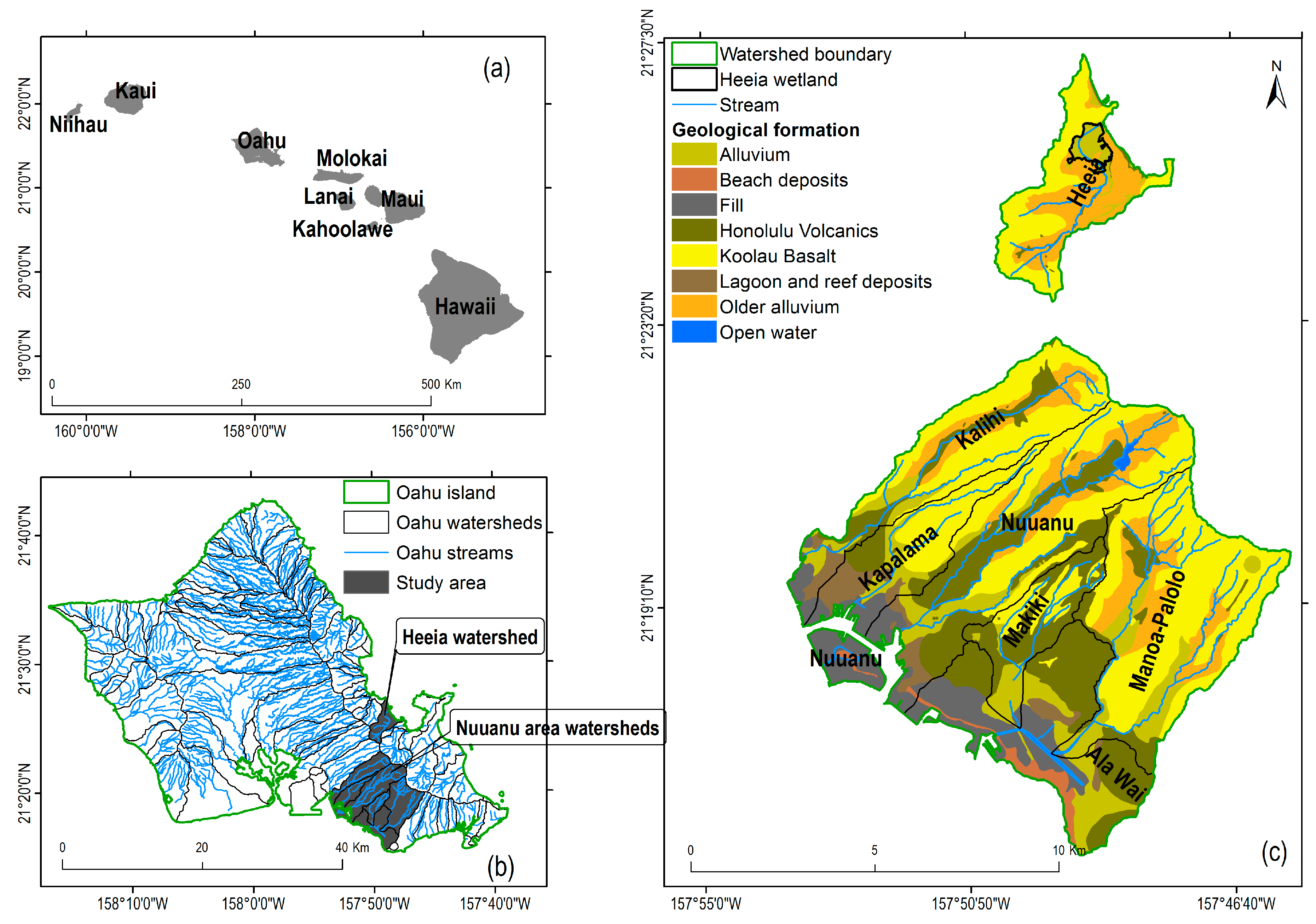
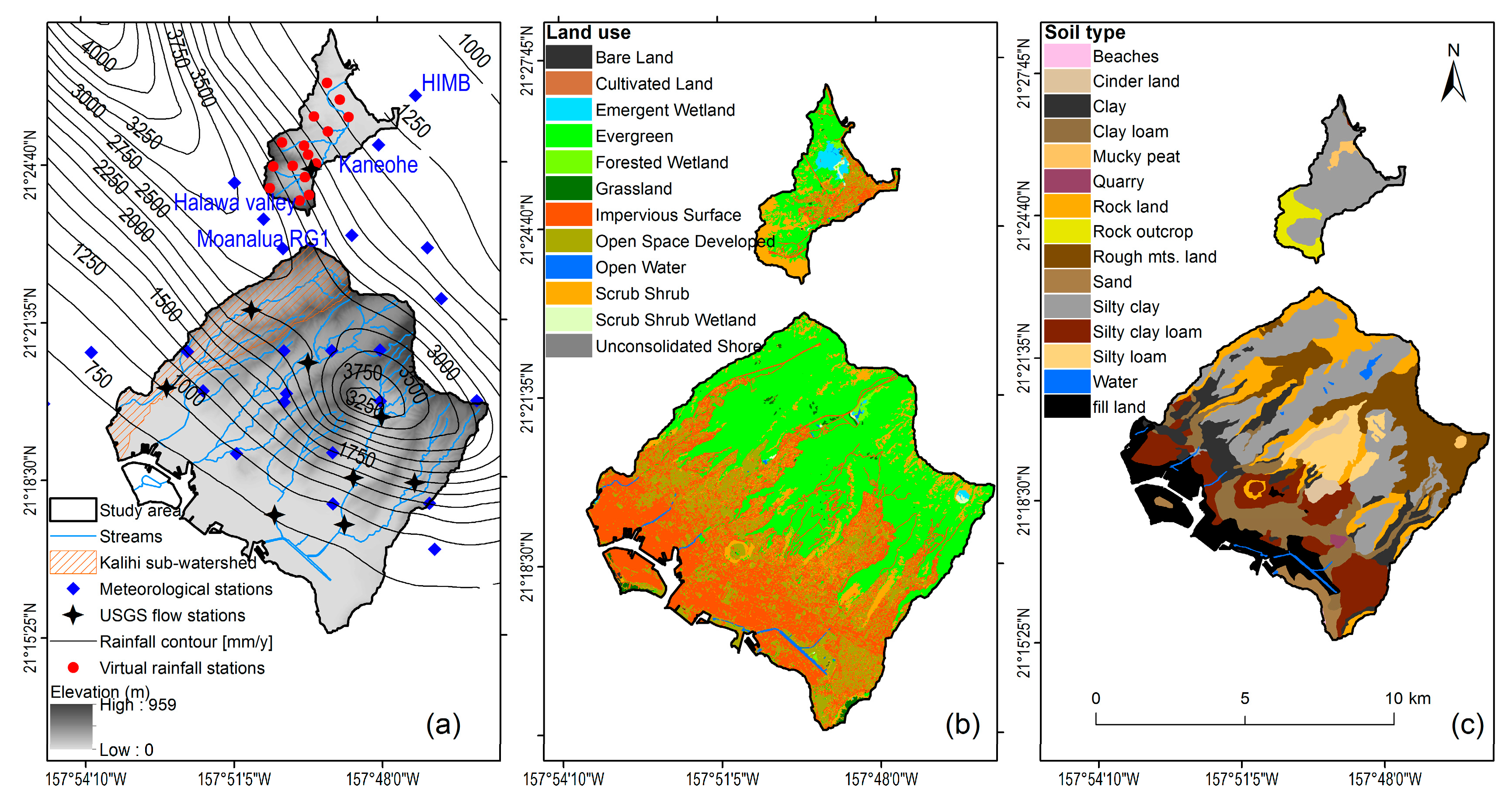
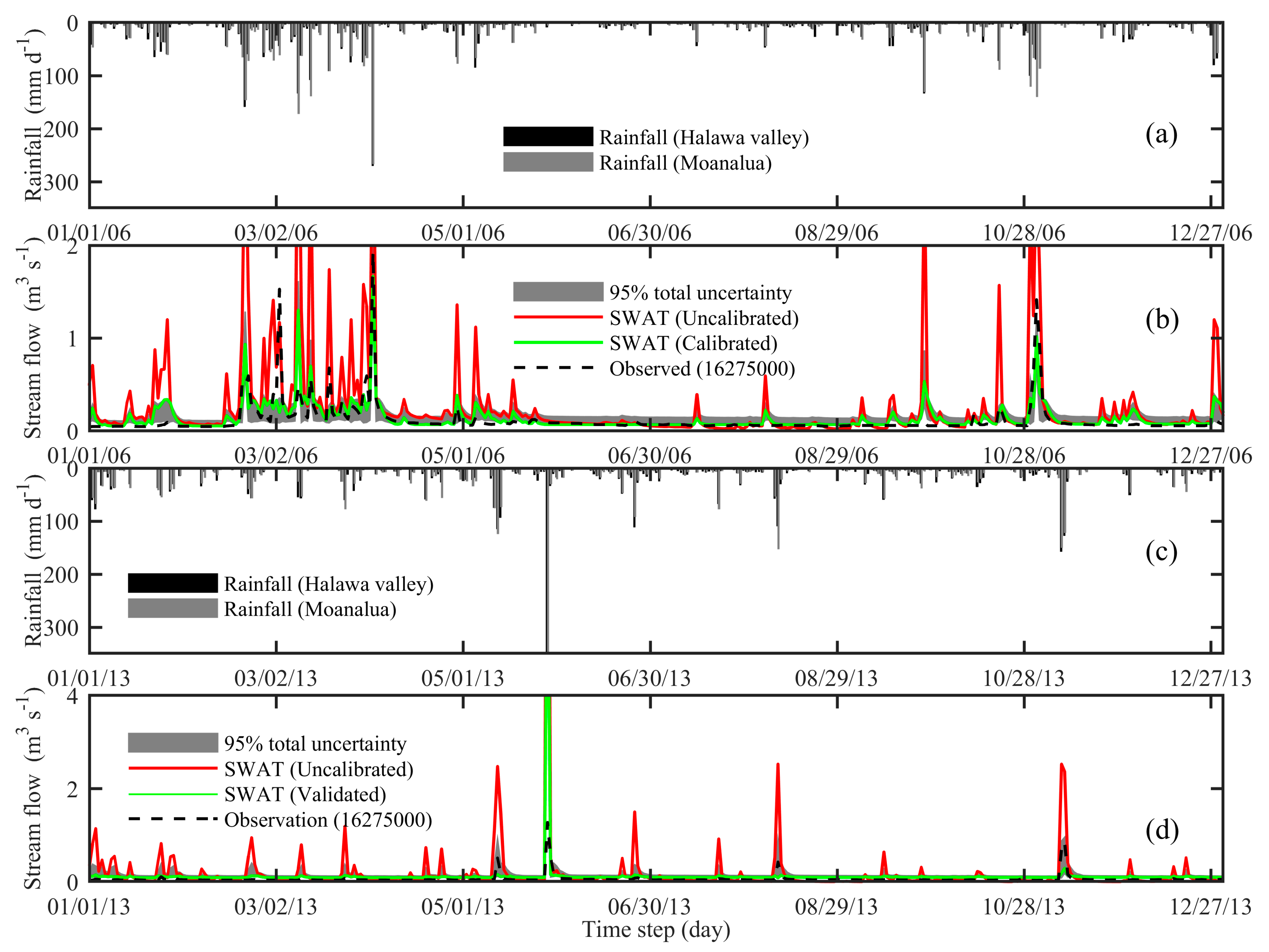
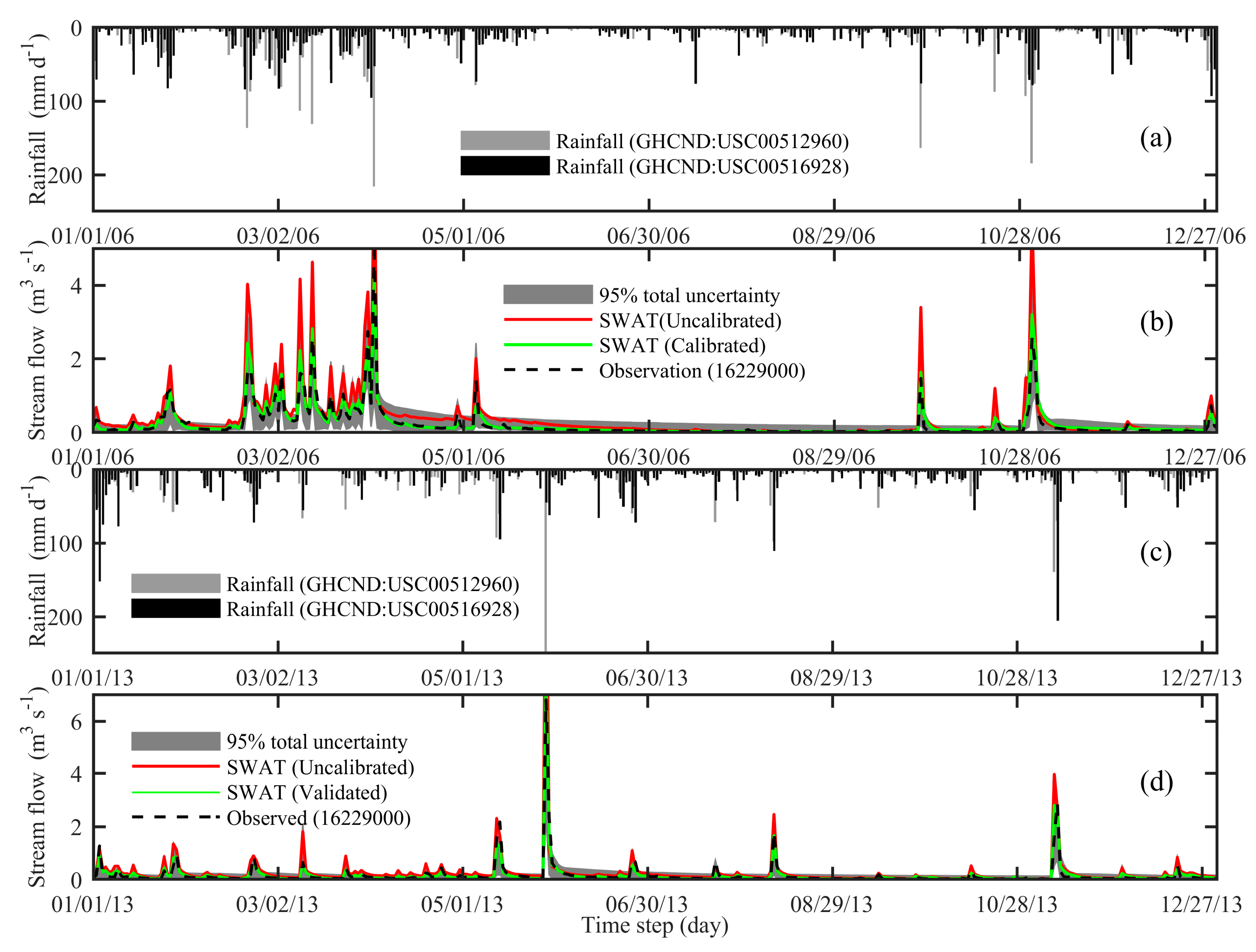
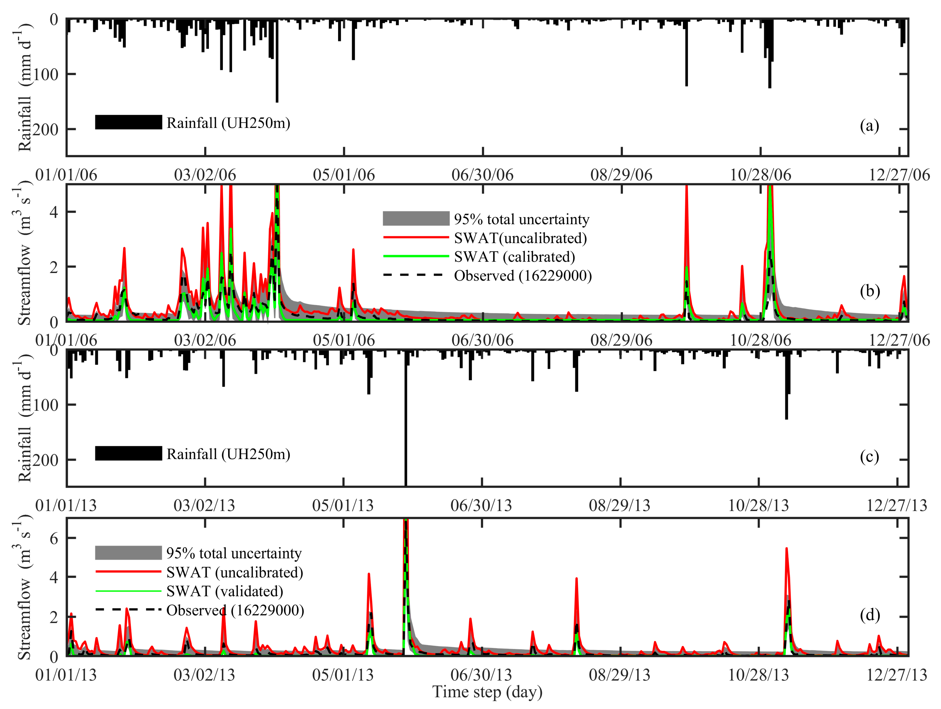
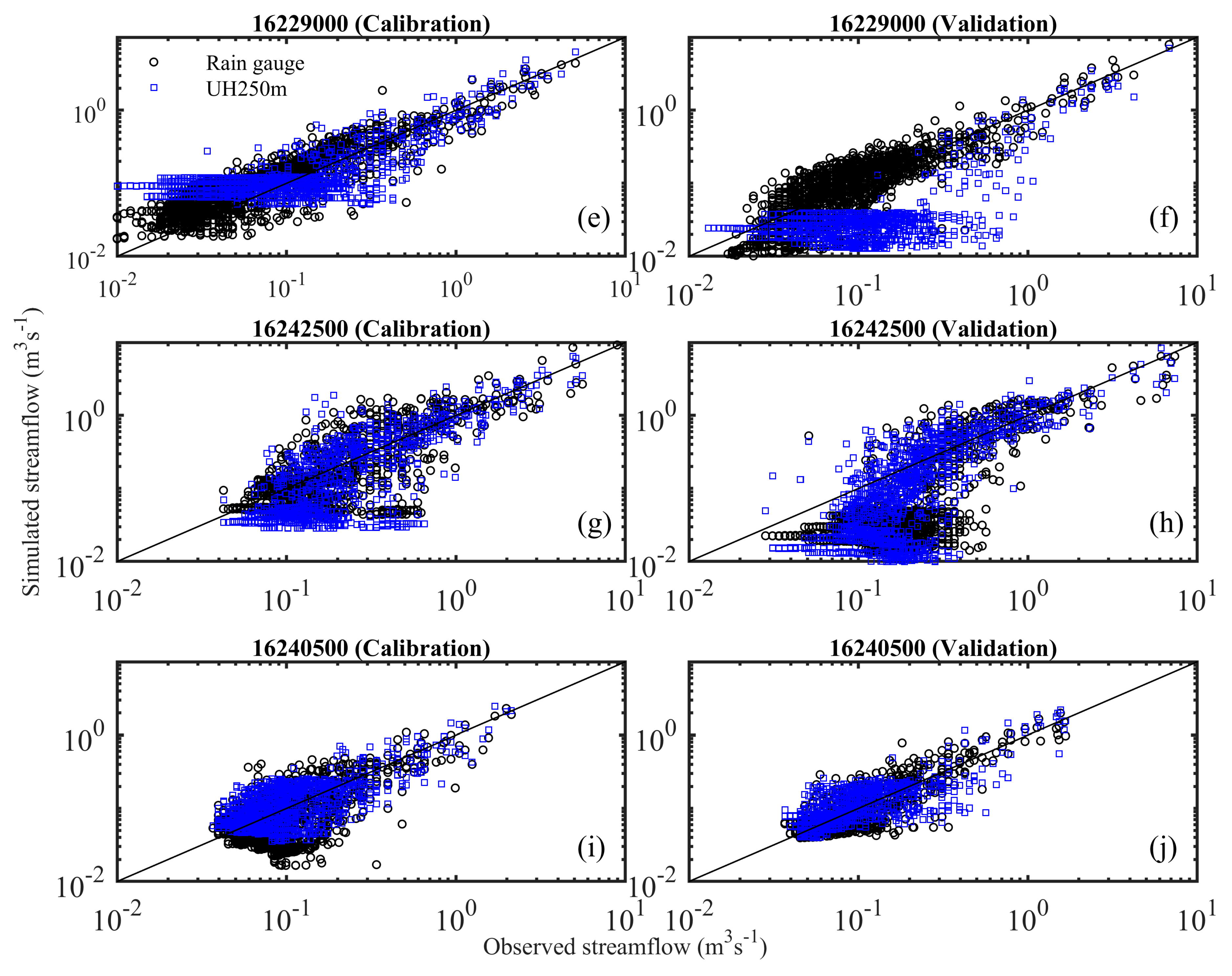
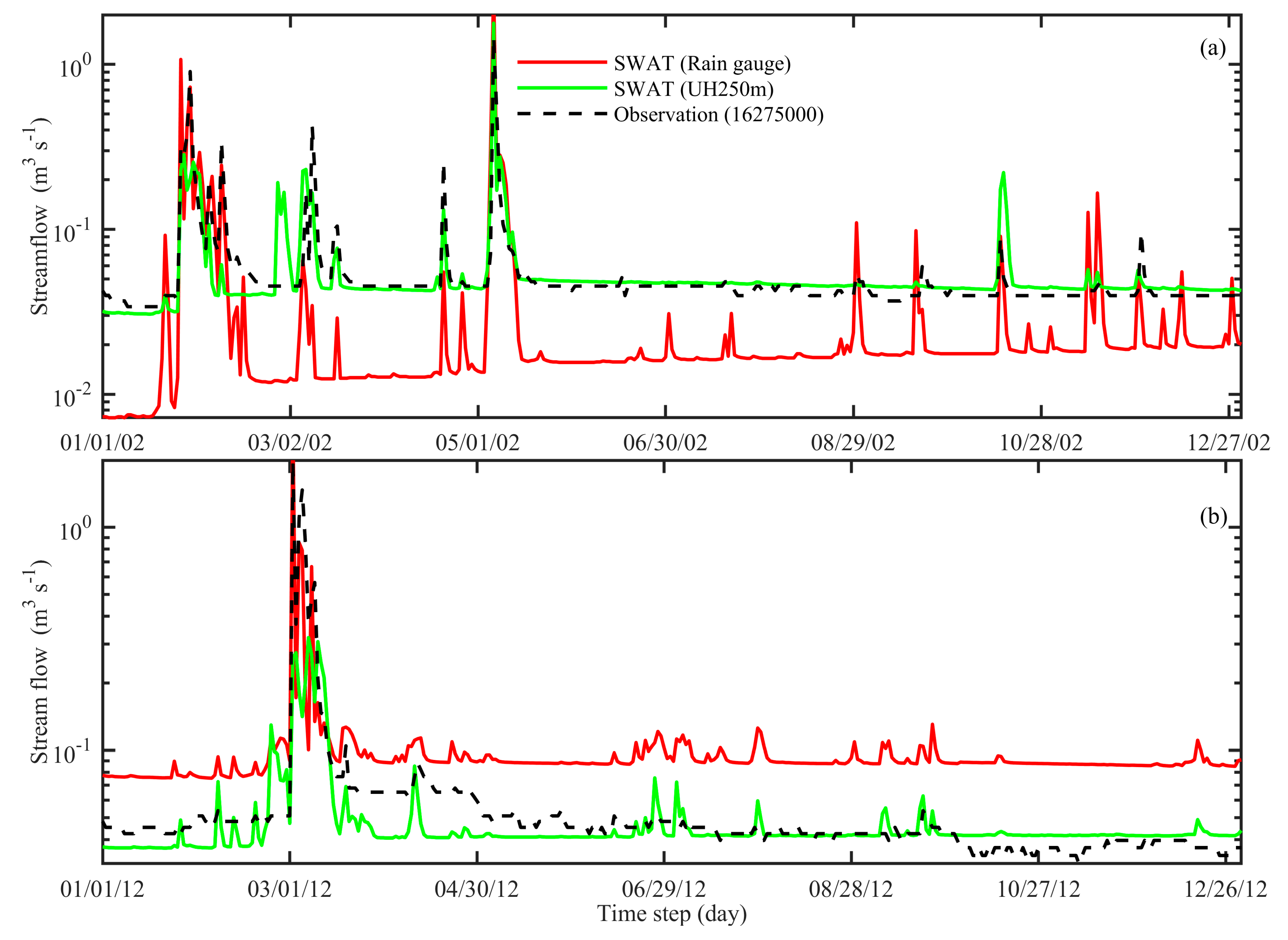
Table 1.
Meteorological stations of SWAT for Heeia and Nuuanu area watersheds.
| Climate Type | Description | Station ID | Resolution | Elevation (m) | Lat. | Long. | Available Period | Source |
|---|---|---|---|---|---|---|---|---|
| Rainfall | BERETANIA PUMP STATION 7 HI US | GHCND:USC00510211 | Daily | 6.1 | 21.317 | −157.850 | 1/1/1980 to present | NOAA-NCDC a |
| HONOLULU INTERNATIONAL AIRPORT HI US | GHCND:USW00022521 | Daily | 2.1 | 21.333 | −157.917 | 1/1/1980 to present | NOAA-NCDC | |
| HONOLULU 2.2 NW HI US | GHCND:US1HIHN0009 | Daily | 126.5 | 21.336 | −157.833 | 18/6/2011 to 1/7/2013 | NOAA-NCDC | |
| HONOLULU 2.7 SSE HI US | GHCND:US1HIHN0010 | Daily | 112.5 | 21.285 | −157.782 | 27/6/2011 to present | NOAA-NCDC | |
| HONOLULU 3.9 WNW HI US | GHCND:US1HIHN0013 | Daily | 105.8 | 21.337 | −157.861 | 6/12/2012 to 12/18/2014 | NOAA-NCDC | |
| KALIHI RES SITE 777 HI US | GHCND:USC00512960 | Daily | 278.0 | 21.383 | −157.833 | 1/1/1980 to present | NOAA-NCDC | |
| KAPALAMA 773 HI US | GHCND:USC00513268 | Daily | 185.9 | 21.350 | −157.867 | 1/1/1980 to present | NOAA-NCDC | |
| MANOA 712.1 HI US | GHCND:USC00516122 | Daily | 6.1 | 21.350 | −157.900 | 1/1/1980 to present | NOAA-NCDC | |
| MANOA LYON ARBO 785.2 HI US | GHCND:USC00516128 | Daily | 153.0 | 21.333 | −157.800 | 1/1/1980 to present | NOAA-NCDC | |
| MANOA TUN 2 716 HI US | GHCND:USC00516130 | Daily | 198.1 | 21.333 | −157.800 | 1/1/1980 to 7/31/2006 | NOAA-NCDC | |
| MOANALUA 770 HI US | GHCND:USC00516395 | Daily | 6.1 | 21.350 | −157.900 | 1/1/1980 to present | NOAA-NCDC | |
| NUUANU RES 4 783 HI US | GHCND:USC00516928 | Daily | 320.0 | 21.350 | −157.817 | 1/1/1980 to present | NOAA-NCDC | |
| NUUANU RES 5 775 HI US | GHCND:USC00516933 | Daily | 125.0 | 21.350 | −157.833 | 1/1/1980 to present | NOAA-NCDC | |
| PALOLO VALLEY 718 HI US | GHCND:USC00517664 | Daily | 305.1 | 21.333 | −157.767 | 1/1/1980 to present | NOAA-NCDC | |
| PAUOA FLATS 784 HI US | GHCND:USC00517810 | Daily | 499.9 | 21.350 | −157.800 | 1/1/1980 to present | NOAA-NCDC | |
| PUNCHBOWL CRATER 709 HI US | GHCND:USC00518316 | Daily | 110.0 | 21.317 | −157.850 | 1/1/1980 to present | NOAA-NCDC | |
| TANTALUS 2 780.5 HI US | GHCND:USC00518738 | Daily | 402.9 | 21.333 | −157.833 | 1/1/1980 to present | NOAA-NCDC | |
| UNIVERSITY OF HAWAII 713 HI US | GHCND:USC00518815 | Daily | 24.1 | 21.300 | −157.817 | 1/1/1980 to present | NOAA-NCDC | |
| WILHELMINA RISE 721 HI US | GHCND:USC00519980 | Daily | 335.9 | 21.300 | −157.783 | 1/1/1980 to present | NOAA-NCDC | |
| KANEOHE 838.1 HI US | GHCND:USC00513117 | Daily | 5.6 | 21.417 | −157.800 | 1/4/1985 to present | NOAA-NCDC | |
| Hawaii Institute of Marine Biology (HIMB) | NA | Daily | 1.0 | 21.433 | −157.787 | 1/9/1992 to present | HIMB | |
| 772.3 Moanalua RG No. 1 at alt 1000 ft, Oahu, HI | 212359157502601 | Daily | 304.8 | 21.393 | −157.840 | 1/1/1978 to present | USGS b | |
| 771.11 N. Halawa Valley RG at tunnel, Oahu, HI | 212428157511201 | Daily | 335.3 | 21.405 | −157.850 | 16/7/1998 to present | USGS | |
| Temperature | HONOLULU INTERNATIONAL AIRPORT HI US | GHCND:USW00022521 | Daily | 2.1 | 21.333 | −157.917 | 1/1/1980 to present | NOAA-NCDC |
| MANOA LYON ARBO 785.2 HI US | GHCND:USC00516128 | Daily | 153.0 | 21.333 | −157.800 | 1/1/1980 to present | NOAA-NCDC | |
| KANEOHE 838.1 HI US | GHCND:USC00513117 | Daily | 18.3 | 21.417 | −157.800 | 1/4/1985 to present | NOAA-NCDC | |
| Hawaii Institute of Marine Biology (HIMB) | NA | Daily | 5.6 | 21.433 | −157.787 | 1/9/1992 to present | HIMB | |
| Wind speed | HONOLULU INTERNATIONAL AIRPORT HI US | GHCND:USW00022521 | Daily | 2.1 | 21.333 | −157.917 | 1/1/1980 to present | NOAA-NCDC |
| KANEOHE 838.1 HI US | GHCND:USC00513117 | Daily | 5.6 | 21.417 | −157.800 | 1/4/1985 to present | NOAA-NCDC | |
| Hawaii Institute of Marine Biology (HIMB) | NA | Daily | 1.0 | 21.433 | −157.787 | 1/9/1992 to present | HIMB | |
| Relative humidity | HONOLULU INTERNATIONAL AIRPORT | 911820/22521 | Hourly | 2.1 | 21.324 | −157.929 | 1/1/1980 to present | NOAA-ISD c |
| Schofield East Hawaii | 325AB384 | Daily | 381.0 | 21.499 | −157.993 | 18/5/2000 to present | WRCC d | |
| Oahu Forest National Weather Research | 8379F6FA | Daily | 698.9 | 21.499 | −157.9 | 25/8/2006 to present | WRCC | |
| Solar radiation | DILLINGHAM HAWAII | 3278D278 | Daily | 30.6 | 21.572 | −158.199 | 1/4/2004 to present | WRCC |
| Hawaii Institute of Marine Biology (HIMB) | NA | Daily | 1.0 | 21.433 | −157.787 | 1/9/1992 to present | HIMB |
a National Oceanic and Atmospheric Administration (NOAA)—National Climatic Data Center; b U.S. Geological Survey; c NOAA Integrated Surface Database; d Western Regional Climate Center.
Table 2.
The performance evaluation criteria (PEC), statistical threshold values, and corresponding assigned weight.
Table 2.
The performance evaluation criteria (PEC), statistical threshold values, and corresponding assigned weight.
| PEC | PBIAS | R2 | NSE | Assigned Weight |
|---|---|---|---|---|
| Very good | PBIAS < ± 5 | R2 > 0.85 | NSE > 0.80 | 4 |
| Good | ±5 ≤ PBIAS < ± 10 | 0.75 < R2 ≤ 0.85 | 0.70 < NSE ≤ 0.80 | 3 |
| Satisfactory | ±10 ≤ PBIAS < ± 15 | 0.60 < R2 ≤ 0.75 | 0.50 < NSE ≤ 0.70 | 2 |
| Unsatisfactory | PBIAS ≥ ±15 | R2 ≤ 0.60 | NSE ≤ 0.50 | 1 |
R2, coefficient of determination; NSE, Nash–Sutcliffe efficiency; PBIAS, percent bias.
Table 3.
Sensitivity rank of SWAT parameters and their corresponding calibrated values for Heeia and Kalihi watersheds.
Table 3.
Sensitivity rank of SWAT parameters and their corresponding calibrated values for Heeia and Kalihi watersheds.
| Parameter | Description | Kalihi (6229000) | Haiku (16275000) | ||||||||||
|---|---|---|---|---|---|---|---|---|---|---|---|---|---|
| Initial-Value | Unit | Rank | t-stat | p-Value | Fitted-RG | Fitted-GRD | Rank | t-stat | p-Value | Fitted-RG | Fitted-GRD | ||
| CN2 | Curve number at moisture condition II a | 55–91 | 1 | −28.12 | 0.000 | −46.50% | −29.90% | 1 | −53.57 | 0.000 | −47.93% | −49.37% | |
| CH_K2 | Effective hydraulic conductivity in main channel | 0.000 | mmh−1 | 2 | 14.50 | 0.000 | 103.500 | 182.500 | 2 | 30.38 | 0.000 | 201.720 | 246.600 |
| ALPHA_BF | Baseflow alpha factor | 0.048 | day−1 | 3 | −4.59 | 0.000 | 0.090 | 0.005 | 3 | −18.18 | 0.000 | 0.001 | 0.001 |
| SOL_AWC | Soil water available capacity b | 0.1–0.18 | 4 | 3.98 | 0.000 | −24.10% | 20.50% | 19 | −0.14 | 0.891 | 12.12% | 24.68% | |
| EPCO | Plant transpiration compensation factor | 1.000 | 5 | 3.28 | 0.001 | 0.810 | 0.623 | 8 | 2.18 | 0.029 | 0.563 | 0.563 | |
| SOL_K | Saturated soil hydraulic conductivity b | 34.2–100.8 | mmh−1 | 7 | 2.30 | 0.022 | 12.10% | −33.70% | 5 | −4.24 | 0.000 | −12.66% | −8.00% |
| REVAPMN | Minimum depth for groundwater revap occurrence | 750.000 | mm | 8 | −2.24 | 0.026 | 175.920 | 15.050 | 12 | −1.45 | 0.147 | 430.250 | 415.75 |
| OV_N | Manning’s roughness coefficient for overland flow a | 0.1–0.15 | 9 | −1.98 | 0.049 | −18.50% | 10.90% | 9 | 1.85 | 0.065 | 6.95% | 5.00% | |
| SOL_Z | Soil depth b | 100–1650 | mm | 10 | 1.88 | 0.060 | 11.70% | −0.71% | 16 | 0.50 | 0.615 | 3.23% | 14.99% |
| GW_REVAP | Groundwater revap coefficient | 0.020 | 0.020 | 11 | 1.66 | 0.098 | 0.180 | 0.028 | 18 | 0.20 | 0.844 | 0.020 | 0.020 |
| ESCO | Soil evaporation compensation factor | 0.950 | 14 | −1.25 | 0.212 | 0.950 | 0.950 | 4 | −5.54 | 0.000 | 0.314 | 0.321 | |
| CH_N2 | Channel Manning’s roughness coefficient | 0.014 | 15 | 0.93 | 0.354 | 0.014 | 0.014 | 6 | 3.97 | 0.000 | 0.035 | 0.035 | |
| GWQMN | Minimum depth for groundwater flow occurrence | 1000.000 | mm | 16 | −0.79 | 0.428 | 1587.500 | 3687.500 | 11 | 1.50 | 0.134 | 2731.50 | 1945.500 |
| CANMX | Maximum canopy storage c | 0.0–8.0 | mm | 19 | −0.08 | 0.940 | 0.0–8.0 | 0.0–8.0 | 10 | 1.73 | 0.085 | 4.0–8.0 | 4.0–8.0 |
| SLSUBBSN | Average sub-basin slope length | 9.0–92.0 | m | 20 | −0.07 | 0.947 | 9.0–92.0 | 9.0–92.0 | 7 | 2.22 | 0.027 | 9.0–92.0 | 9.0–92.0 |
a varies with land use, soil, and slope; b varies with soil type; c varies with land use, but set to zero for urban land use; RG, Rain gauges data; GRD, Gridded rainfall data.
Table 4.
Observed and simulated annual average streamflow, surface runoff (SR), and subsurface flow (SSF) (in mm) and percentages of SR and SSF relative to total streamflow for Heeia and Kalihi. Bold signifies unsatisfactory.
Table 4.
Observed and simulated annual average streamflow, surface runoff (SR), and subsurface flow (SSF) (in mm) and percentages of SR and SSF relative to total streamflow for Heeia and Kalihi. Bold signifies unsatisfactory.
| Watershed | Station | Period | Type | Streamflow | SR | Subsurface Flow |
|---|---|---|---|---|---|---|
| Heeia | 16275000 | 2002–2008 | Observed | 994 | 303 | 691 |
| Sensitivity analysis (SA) | 1622 | 333 | 1289 | |||
| Calibration | 1059 | 390 | 669 | |||
| Percent (Observed) a | NA | 31 | 69 | |||
| Percent (SA) | NA | 21 | 79 | |||
| Percent (Calibration) | NA | 37 | 63 | |||
| PBIAS (SA) | 63.2 | 9.8 | 86.6 | |||
| PBIAS (Calibration) | 6.5 | 28.7 | −3.2 | |||
| Kalihi | 16229000 | 2006–2010 | Observed | 680 | 302 | 378 |
| Sensitivity analysis (SA) | 990 | 260 | 730 | |||
| Calibration | 780 | 360 | 420 | |||
| Percent (Observed) | NA | 44 | 56 | |||
| Percent (SA) | NA | 26 | 74 | |||
| Percent (Calibration) | NA | 46 | 54 | |||
| PBIAS (SA) | 45.5 | −13.9 | 92.8 | |||
| PBIAS (Calibration) | 14.7 | 19.1 | 11.1 |
a Percent was calculated relative to the total annual streamflow values.
Table 5.
Goodness-of-fit statistics for daily streamflow simulations at Heeia and Nuuanu area watersheds using rain gauge data. Bold signifies unsatisfactory.
Table 5.
Goodness-of-fit statistics for daily streamflow simulations at Heeia and Nuuanu area watersheds using rain gauge data. Bold signifies unsatisfactory.
| Watershed | Station No. | Period | Time Span | Behavioral No. | p-factor | r-factor | NSE | R2 | PBIAS (%) | Assigned Weight | Overall | |||
|---|---|---|---|---|---|---|---|---|---|---|---|---|---|---|
| NSE | R2 | PBIAS | Average | Ratings | ||||||||||
| Heeia | 16275000 | Uncalibration | 2002–2008 | NA | NA | NA | −6.87 | 0.55 | 98.4 | 1.0 | 1.0 | 1.0 | 1.0 | Unsatisfactory |
| Calibration | 2002–2008 | 78 | 0.57 | 0.63 | 0.39 | 0.48 | 6.5 | 1.0 | 1.0 | 4.0 | 2.0 | Satisfactory | ||
| Validation | 2009–2013 | 0 | 0.40 | 1.11 | −2.00 | 0.29 | 20.3 | 1.0 | 1.0 | 1.0 | 1.0 | Unsatisfactory | ||
| NA | Uncalibration | 2002–2008 | NA | NA | NA | −1.45 | 0.62 | 30.83 | 1.0 | 2.0 | 1.0 | 1.3 | Unsatisfactory | |
| Calibration | 2002–2008 | 420 | 0.79 | 0.67 | 0.66 | 0.66 | −11.5 | 2.0 | 2.0 | 3.0 | 2.3 | Satisfactory | ||
| Validation | 2009–2013 | 221 | 0.82 | 0.47 | 0.53 | 0.56 | −1.6 | 2.0 | 1.0 | 4.0 | 2.3 | Satisfactory | ||
| Kalihi | 16229000 | Uncalibration | 2006–2010 | NA | NA | NA | −0.07 | 0.86 | 77.09 | 1.0 | 4.0 | 1.0 | 2.0 | Satisfactory |
| Calibration | 2006–2010 | 299 | 0.83 | 0.84 | 0.86 | 0.86 | 14.66 | 4.0 | 4.0 | 2.0 | 3.3 | Good | ||
| Validation | 2011–2014 | 344 | 0.93 | 0.72 | 0.88 | 0.88 | 1.10 | 4.0 | 4.0 | 4.0 | 4.0 | Very good | ||
| Nuuanu | 16232000 | Uncalibration | 1990–1995 | NA | NA | NA | −2.55 | 0.74 | 221.93 | 1.0 | 2.0 | 1.0 | 1.3 | Unsatisfactory |
| Calibration | 1990–1995 | 303 | 0.93 | 0.78 | 0.72 | 0.76 | 8.80 | 3.0 | 3.0 | 3.0 | 3.0 | Good | ||
| Validation | 1985–1989 | 360 | 0.90 | 0.46 | 0.58 | 0.59 | 11.30 | 2.0 | 1.0 | 2.0 | 1.7 | Satisfactory | ||
| Makiki | 16238000 | Uncalibration | 2010–2012 | NA | NA | NA | −3.14 | 0.70 | 30.11 | 1.0 | 2.0 | 1.0 | 1.3 | Unsatisfactory |
| Calibration | 2010–2012 | 32a | 0.91 | 0.49 | 0.65 | 0.76 | −4.70 | 2.0 | 3.0 | 4.0 | 3.0 | Good | ||
| Validation | 2013–2014 | 3a | 0.94 | 1.99 | 0.57 | 0.66 | −8.40 | 2.0 | 2.0 | 3.0 | 2.3 | Satisfactory | ||
| Manoa-Palolo | 16240500 | Uncalibration | 2006–2010 | NA | NA | NA | −1.38 | 0.77 | 68.42 | 1.0 | 3.0 | 1.0 | 1.7 | Satisfactory |
| Calibration | 2006–2010 | 102 | 0.85 | 0.89 | 0.71 | 0.72 | −1.30 | 3.0 | 2.0 | 4.0 | 3.0 | Good | ||
| Validation | 2011–2014 | 21 | 0.95 | 0.81 | 0.79 | 0.81 | −1.40 | 3.0 | 3.0 | 4.0 | 3.3 | Good | ||
| 16242500 | Uncalibration | 2006–2010 | NA | NA | NA | −1.61 | 0.76 | 130.80 | 1.0 | 3.0 | 1.0 | 1.7 | Satisfactory | |
| Calibration | 2006–2010 | 417 | 0.94 | 0.91 | 0.71 | 0.72 | −3.20 | 3.0 | 2.0 | 4.0 | 3.0 | Good | ||
| Validation | 2011–2014 | 418 | 0.97 | 0.91 | 0.75 | 0.77 | −21.70 | 3.0 | 3.0 | 1.0 | 2.3 | Satisfactory | ||
| 16244000 | Uncalibration | 2010–2012 | NA | NA | NA | −1.83 | 0.73 | 286.09 | 1.0 | 2.0 | 1.0 | 1.3 | Unsatisfactory | |
| Calibration | 2010–2012 | 8 a | 0.93 | 1.17 | 0.63 | 0.64 | 15.80 | 2.0 | 2.0 | 1.0 | 1.7 | Satisfactory | ||
| Validation | 2013–2014 | 343 | 0.71 | 0.77 | 0.83 | 0.81 | 18.20 | 4.0 | 3.0 | 1.0 | 2.7 | Good | ||
a There are more than 200 behavioral solutions if NSE is set to ≥0.2 (similar to Heeia watershed). Behavioral solutions of Nuuanu area watershed were calculated at NSE ≥ 0.5. p-factor, percent of observations bracketed at 95% confidence interval (95PCI); r-factor, average width of 95PCI; NSE, Nash–Sutcliffe efficiency; R2, coefficient of determination; PBIAS, percent bias; NA = Not Available.
Table 6.
Goodness-of-fit statistics for daily streamflow simulations at Heeia and Nuuanu area watersheds using UH250m rainfall data. Bold signifies unsatisfactory.
Table 6.
Goodness-of-fit statistics for daily streamflow simulations at Heeia and Nuuanu area watersheds using UH250m rainfall data. Bold signifies unsatisfactory.
| Watershed | Station No. | Period | Time Span | Behavioral No. | p-factor | r-factor | NSE | R2 | PBIAS (%) | Assigned Weight | Overall | |||
|---|---|---|---|---|---|---|---|---|---|---|---|---|---|---|
| NSE | R2 | PBIAS | Average | Ratings | ||||||||||
| Heeia | Uncalibration | 2002–2008 | NA | NA | NA | −3.96 | 0.66 | 56.8 | 1.0 | 2.0 | 1.0 | 1.3 | Unsatisfactory | |
| 16275000 | Calibration | 2002–2008 | 437 | 0.73 | 0.59 | 0.50 | 0.53 | 15.8 | 1.0 | 1.0 | 3.0 | 1.7 | Satisfactory | |
| Validation | 2009–2013 | 226 | 0.68 | 0.61 | 0.38 | 0.40 | −22.4 | 1.0 | 1.0 | 2.0 | 1.3 | Unsatisfactory | ||
| Uncalibration | 2002–2008 | NA | NA | NA | −2.01 | 0.64 | 27.4 | 1.0 | 2.0 | 1.0 | 1.3 | Unsatisfactory | ||
| NA | Calibration | 2002–2008 | 405 | 0.89 | 0.71 | 0.60 | 0.61 | −5.2 | 2.0 | 2.0 | 4.0 | 2.7 | Good | |
| Validation | 2009–2013 | 333 | 0.94 | 0.64 | 0.62 | 0.62 | −5.5 | 2.0 | 2.0 | 4.0 | 2.7 | Good | ||
| Kalihi | 16229000 | Uncalibration | 2006–2010 | NA | NA | NA | −1.34 | 0.84 | 134.2 | 1.0 | 3.0 | 1.0 | 1.7 | Satisfactory |
| Calibration | 2006–2010 | 99 | 0.46 | 0.89 | 0.80 | 0.82 | 13.7 | 3.0 | 3.0 | 3.0 | 3.0 | Good | ||
| Validation | 2011–2014 | 112 | 0.57 | 0.84 | 0.78 | 0.83 | −53.6 | 3.0 | 3.0 | 1.0 | 2.3 | Satisfactory | ||
| Nuuanu | 16232000 | Uncalibration | 1992–1995 | NA | NA | NA | −0.32 | 0.67 | 118.6 | 1.0 | 2.0 | 1.0 | 1.3 | Unsatisfactory |
| Calibration | 1992–1995 | 430 | 0.78 | 0.54 | 0.74 | 0.75 | 2.1 | 3.0 | 2.0 | 4.0 | 3.0 | Good | ||
| Validation | NA | NA | NA | NA | NA | NA | NA | NA | NA | NA | NA | NA | ||
| Makiki | 16238000 | Uncalibration | 2010–2012 | NA | NA | NA | −4.47 | 0.73 | 183.1 | 1.0 | 2.0 | 1.0 | 1.3 | Unsatisfactory |
| Calibration | 2010–2012 | 3a | 0.70 | 0.26 | 0.62 | 0.67 | −36.0 | 2.0 | 2.0 | 1.0 | 1.7 | Satisfactory | ||
| Validation | 2013–2014 | 0a | 0.55 | 2.17 | 0.24 | 0.44 | −72.4 | 1.0 | 1.0 | 1.0 | 1.0 | Unsatisfactory | ||
| Manoa-Palolo | 16240500 | Uncalibration | 2006–2010 | NA | NA | NA | −1.18 | 0.81 | 49.1 | 1.0 | 3.0 | 1.0 | 1.7 | Satisfactory |
| Calibration | 2006–2010 | 108 | 0.82 | 0.83 | 0.69 | 0.72 | 6.9 | 2.0 | 2.0 | 4.0 | 2.7 | Good | ||
| Validation | 2011–2014 | 55 | 0.87 | 0.88 | 0.68 | 0.74 | 7.4 | 2.0 | 2.0 | 4.0 | 2.7 | Good | ||
| 16242500 | Uncalibration | 2006–2010 | NA | NA | NA | −0.15 | 0.85 | 75.6 | 1.0 | 3.0 | 1.0 | 1.7 | Satisfactory | |
| Calibration | 2006–2010 | 496 | 0.87 | 0.65 | 0.83 | 0.85 | −11.0 | 4.0 | 3.0 | 3.0 | 3.3 | Good | ||
| Validation | 2011–2014 | 484 | 0.93 | 0.72 | 0.74 | 0.75 | −18.9 | 3.0 | 2.0 | 2.0 | 2.3 | Satisfactory | ||
| 16244000 | Uncalibration | 2010–2012 | NA | NA | NA | −4.74 | 0.78 | 337.2 | 1.0 | 2.0 | 1.0 | 1.3 | Unsatisfactory | |
| Calibration | 2010–2012 | 3 a | 0.87 | 0.39 | 0.65 | 0.80 | −30.0 | 2.0 | 3.0 | 1.0 | 2.0 | Satisfactory | ||
| Validation | 2013–2014 | 7 a | 0.90 | 0.50 | 0.72 | 0.73 | 14.7 | 3.0 | 2.0 | 3.0 | 2.7 | Good | ||
a Behavioral solutions of Nuuanu area watershed were calculated at NSE ≥ 0.5 and could be more if set to 0.2 (similar to Heeia watershed). p-factor, percent of observations bracketed at 95% confidence interval (95PCI); r-factor, average width of 95PCI; NSE, Nash–Sutcliffe efficiency; R2, coefficient of determination; PBIAS, percent bias; NA = Not Available.
© 2018 by the authors. Licensee MDPI, Basel, Switzerland. This article is an open access article distributed under the terms and conditions of the Creative Commons Attribution (CC BY) license (http://creativecommons.org/licenses/by/4.0/).
Share and Cite
MDPI and ACS Style
Leta, O.T.; El-Kadi, A.I.; Dulai, H.; Ghazal, K.A. Assessment of SWAT Model Performance in Simulating Daily Streamflow under Rainfall Data Scarcity in Pacific Island Watersheds. Water 2018, 10, 1533. https://doi.org/10.3390/w10111533
AMA Style
Leta OT, El-Kadi AI, Dulai H, Ghazal KA. Assessment of SWAT Model Performance in Simulating Daily Streamflow under Rainfall Data Scarcity in Pacific Island Watersheds. Water. 2018; 10(11):1533. https://doi.org/10.3390/w10111533
Chicago/Turabian StyleLeta, Olkeba Tolessa, Aly I. El-Kadi, Henrietta Dulai, and Kariem A. Ghazal. 2018. "Assessment of SWAT Model Performance in Simulating Daily Streamflow under Rainfall Data Scarcity in Pacific Island Watersheds" Water 10, no. 11: 1533. https://doi.org/10.3390/w10111533
Note that from the first issue of 2016, this journal uses article numbers instead of page numbers. See further details here.