Stomatal Conductance Responses of Acacia caven to Seasonal Patterns of Water Availability at Different Soil Depths in a Mediterranean Savanna

Abstract

Soil water availability controls plant productivity in seasonally dry ecosystems, although plant water use at different soil depths and times is, to the best of our knowledge, not clearly understood. Environmental variables at the canopy level and the soil volumetric water content (VWC) at five different soil depths were continuously recorded for three years (2011–2014) in an Acacia caven savanna site in central Chile. Stomatal conductance ($g_s$) was measured every hour during daytime for 42 days distributed across the study period. Values of $g_s$ were weakly controlled by photosynthetically active radiation, vapor pressure deficit, and leaf temperature when considering the whole series. The variance proportion being explained increased from 5% to 20% if the whole series was partitioned into a dry and a wet season. According to the above, A. caven exhibited a more anisohydric behavior than previously thought. When we added the VWC in the root zone, to the $g_s$ atmospheric variables model, R² increased to 47% when separately considering the dry and wet seasons. However, we did not find a differentiated use of water in the root zone, but instead a joint activity of the radicular system within the top 100 cm of the soil controlling $g_s$.

1. Introduction

In seasonally dry ecosystems, such as those of central Chile, water is the limiting factor for vegetation growth and survival [1,2,3,4]. Plant productivity is a process intimately controlled by stomatal aperture [5,6,7], which is commonly measured as leaf stomatal conductance ($g_s$) and expressed as mmol H₂O per m² of leaf area and second, per unit change in air vapor pressure deficit (D) [8,9]. Stomatal conductance promptly responds to changes in the water content in the atmosphere and soil [10], therefore regulating the relation between the processes of transpiration and assimilation [11,12]. However, there are only a few field observations of $g_s$, which, together with other measurements such as predawn and midday plant water potential, may assist to determine whether A. caven exhibits an isohydric or anisohydric behavior.

Stomatal conductance has a strong dependence on the availability of water in the root zone [13,14,15,16]. Such dependence can be examined by at least two approaches: a microscopic approach focused on a detailed analysis of radicular function during water capture, and a macroscopic one where the entire radicular system is treated as a unit; that is, the dynamics of the water within the soil correspond to the sum of the effects on the whole root. However, an intermediate approach can be implemented because the desiccation of the soil during periods without rain is more pronounced in the superficial layers than deeper in the soil [15,16].

Oren et al. [17] showed that the plant water potential of adult Pinus taeda trees would be conditioned by the equilibrium between leaf stomatal conductance ($g_s$) and the soil water content (VWC) at 30 and 50 cm depths. Similarly, Irvine et al. [18] noted that 54% of water extracted from the soil is removed from the first 50 cm in the root zone driven by transpiration, and that stomatal conductance exhibited a positive linear response with respect to the total amount of available water when the soil volumetric water content was between 5% and 12% in adult Pinus silvestris trees during dry periods. Stewart [19] showed that $g_s$ for Pinus species starts to decline when the soil water content at 90 cm depth reaches <5%, with 0% representing the hygroscopic point for the soil, or minimum water content and 100% field capacity. Gu et al. [20] reported that, unlike the species mentioned above, those associated with woody shrub formations are able to capture water from the soil in an adaptive manner from both superficial and deeper layers under water stress conditions. Despite that report, the impact of soil moisture distribution in the root zone over the $g_s$ of vegetation exposed to marked seasonal changes has been rarely studied [15,19,21,22], although arid and semi-arid zones cover around two-thirds of the terrestrial area [23].

Anav et al. [16] showed that a decrease in soil water content in the root zone associated with recurrent droughts caused a decline of stomatal conductance followed, in extreme cases, by foliage shedding or branch death. According to the authors, this effect is more marked in Mediterranean semi-arid environments. In Chile, this ecosystem extends between latitudes of 30° and 36° S, covers approximately two million hectares and is represented by a woody community of Acacia caven (Mol.) Mol and annual herbs [24,25,26]. According to Schulz et al. [27] and Van de Wouw et al. [28], this species has rapidly colonized strongly disturbed areas, being the most important agroforest systems in the unirrigated portion of central Chile [25]. For A. caven there is an apparent synchronizing pattern involving the availability of water in the upper soil layer (0–30 cm) and $g_s$, which is typical of isohydric species [29]. Such response makes this species particularly well suited to study the short-term $g_s$ responses to seasonal changes in atmospheric conditions and soil water content at different soil depths.

Our ability to predict long term plant responses in seasonally dry ecosystems to the increase in hydrological variability depends critically on our ability to better understand, interpret and scale local and short-term responses to larger spatial and longer temporal scales. According to the above, we hypothesize that A. caven maintains high stomatal conductance even under dry and hot atmospheric conditions, while differentially using water from different soil depths. We aimed to test whether the temporal variability of stomatal conductance ($g_s$) can be better explained if both the seasonality of the atmospheric variables and the vertical dynamics of the volumetric water content (VWC) are incorporated. Our questions in this regard are the following: (1) What is the gain in temporal $g_s$ representation when seasonality and the vertical distribution of water in the root zone are incorporated? (2) At what depth in the root zone does the stored water significantly impact the $g_s$ representation?

2. Materials and Methods

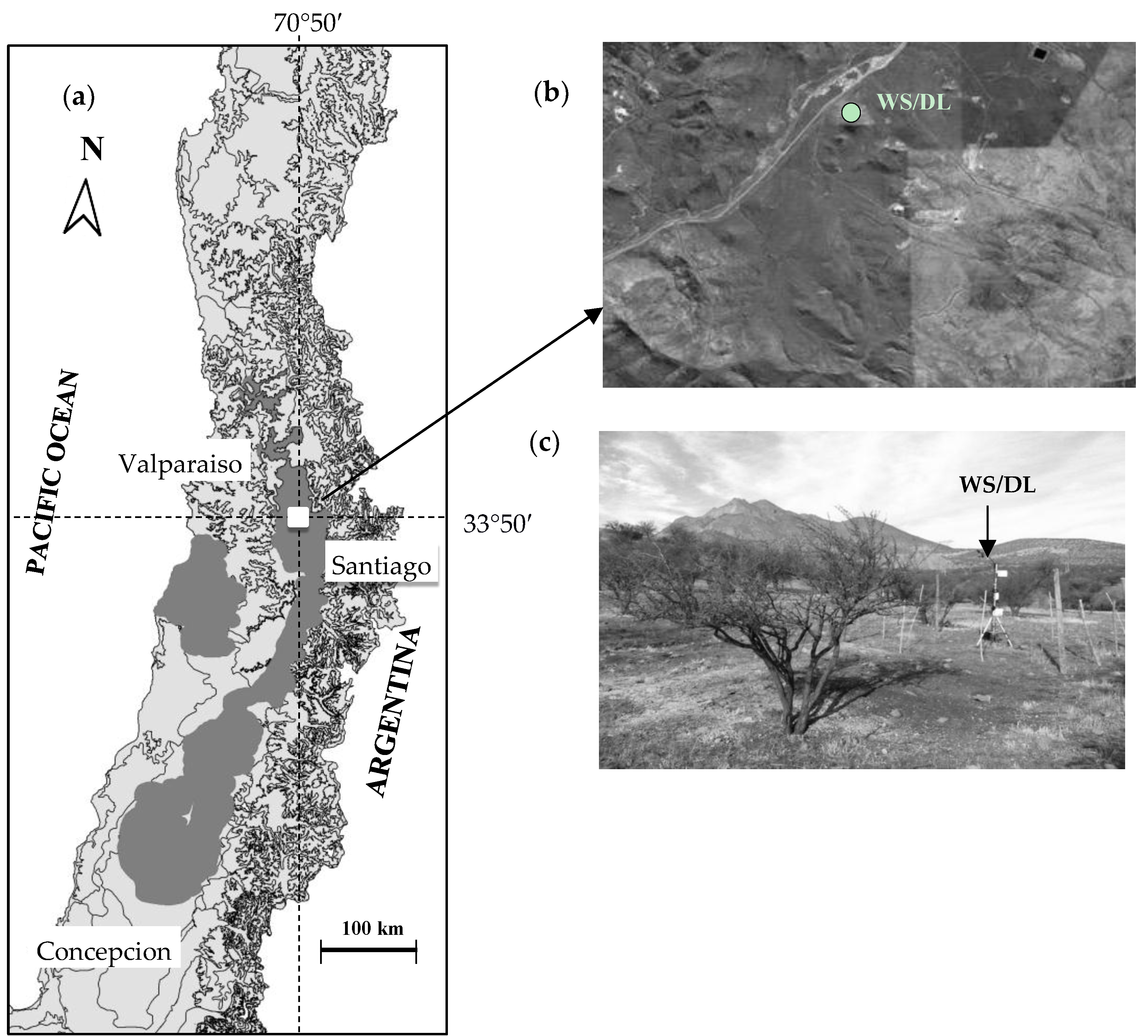
2.1. Study Area

The studied site was located at latitude 33°50′ S and longitude 70°50′ W, 550 m above the sea level, 50 km north of the city of Santiago, Chile (Figure 1). According to Peel et al. [30], the climate is Mediterranean with a warm dry season (Csa, a Koppen classification and corresponds to “Hot-summer mediterranean climate”) lasting from 7 to 8 months, where the potential evapotranspiration (1100 mm·year⁻¹) far exceeds the precipitation (289 mm·year⁻¹). The mean annual temperature during the period 2000–2014 was 14.5 °C, with maximum values in January (~30 °C) and minimums in July (~2 C). According to the Meteorological Office of Chile, the long-term mean annual precipitation (MAP) in the past 50 years (period 1964–2014) was 289 mm·year⁻¹, with a minimum of 53 mm·year⁻¹ (1968) and a maximum of 820 mm·year⁻¹ (1987).

The study site (Figure 1c) was relatively homogeneous in terms of vegetation, soil, land form and aspect [31]. We selected a homogeneous site of about 20 ha where Acacia caven was the woody dominant species. The plant community was made out of two strata configuring a savanna landscape. The first stratum provides soil coverage of 5% to 10%, composed mainly of two perennial species: Acacia caven, sporadically accompanied by Lithraea caustica (Molina) Hook. & Arn. The second has an additional soil coverage between 5% and 7%, increasing to a maximum of about 35% for a brief period early in the dry season, being composed of annual herbs dominated by slender wild oat (Avena barbata Pott ex Link). We observed a few isolated shrubs of Flourensia thurifera (Mol.) DC and Proustia cinerea D. Don. Because the site has not been disturbed by human activities since the early 1990s, we assumed that $g_s$ responses would be mainly controlled by atmospheric and soil conditions rather than other factors such as disturbance.

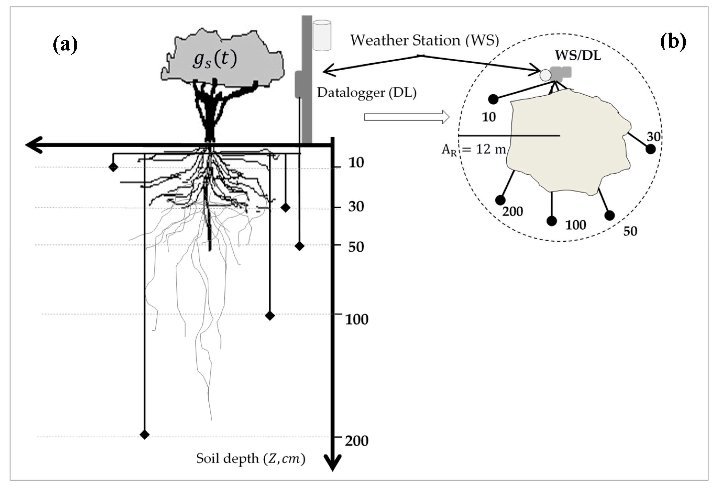
2.2. Recording the Microclimate Variables at the Site

Soil description of the site was based on 4 randomly located pits of 1 m × 1 m and variable depths which were dug during 7–8 June 2011, after three major rainfall events (1 in April and 2 in May). From these pits, we obtained bulked samples of about 1 kg, following the protocols suggested by the Soil and Plant Laboratory of the Pontificia Universidad Católica de Chile, at 5 different depths: 10, 30, 50, 100, and 200 cm, which were analyzed for soil texture, bulk density, field capacity (FC) and permanent wilting point (PWP). Soil depth of the root zone was measured at the pit based on the presence or absence of roots for the different soil horizons.

Environmental conditions at the study site were recorded with a micro-meteorological station (WS) mounted on a metallic stand at 3.5 m in height, being approximately 0.5 m over the maximum height of the A. caven trees. Precipitation, wind velocity, solar radiation in the visible spectrum (400–700 nm), air temperature, and relative humidity were recorded every 5 min using a high-resolution rain gauge (ECRN-100, Decagon Devices, Pullman, WA, USA), an anemometer, a photosynthetically active radiation (PAR) Quantum Sensor QSO, and a Temperature/Relative Humidity Sensor (EHT, Decagon Devices, Pullman, WA, USA), respectively. Vapor pressure deficit (VPD) was calculated from $T_{air}$ and $R{H}_{air}$ according to Allen et al. [32] and Abtew and Melesse [33].

The soil volumetric water content (soil VWC) was recorded with frequency domain reflectometry (FDR) type sensors (model 5TM, Decagon Devices, Pullman, WA, USA) placed at 5 different soil depths: 10, 30, 50, 100 and 200 cm (Figure 2). FDR sensors were calibrated before starting the experiment by taking soil samples and measuring soil water content by the gravimetric method. The bulk density was determined using the paraffin-sealed clod method [34]. We choose the mineral soil calibration option in the Decagon’s ProCheck reader, in the ECH2O Utility Software (Decagon Devices, Pullman, WA, USA), because it converts raw dielectric permittivity values using the Topp equation. The Topp equation resulted in measurements within ±3% of the VWC determined using the gravimetric method. Additionally, we recorded soil VWC in 3 points around the micro-meteorological station using a FieldScout™ TDR 300 (Spectrum Technologies Inc., Aurora, IL, USA) to 20 cm in soil depth in a high clay mode, to contrast with the records in the middle root zone taken by the micrometeorological station. These records were made during 7 days in the wet season and 9 days in the dry season between 2011 and 2013. We found that the VWC measurements taken at 20 cm with the TDR 300 were not significantly different from those taken with the FDR at 30 cm (Figure S1).

2.3. Stomatal Conductance Measurements

Four mid-crown measurements of stomatal conductance ($g_s$) were made on 15 selected A. caven trees over 42 days spread within the period 24 July 2011 to 27 December 2013. Within this period, 26 days were in the dry season (October–April) and 16 days in the wet season (May–September). Date and hour of measurement were recorded to match with measurements from the micrometeorological station. Values of $g_s$ were recorded systematically from 7 am to 6 pm, totaling 329 measurements, after taking out invalid records. Measurements were taken with a leaf porometer (model SC-1, Decagon Devices, Pullman, WA, USA), following the protocols suggested by Johnson et al. [35]. The porometer also provided estimates of leaf temperature ($T_L$ in °C) and leaf boundary-layer relative humidity ($R{H}_{leaf}$). In the wet season, $g_s$ measurements were not made on rainy days, or two days following a rain event, and also discarded if air temperature was less than 5 °C as suggested by the manufacturer.

2.4. Statistical Analysis

Data were evaluated using exploratory data analysis, as recommended by Zuur et al. [36]. Taking into consideration the big-leaf approximation, we evaluated the significance of the atmospheric variables on stomatal conductance ($g_s$), through a multiple linear regression analysis (MR) using both the complete series (CS) and a seasonal adjustment (K), that considered a dry and a wet season following Matsumoto et al. [37]. Then, leaf stomatal conductance ($g_s$) was regressed against PAR, VPD, wind velocity ($W_v$), and leaf temperature ($T_{leaf}$), the latter following Urban et al. [38]. Forward stepwise regression was used to include only significant variables by minimizing the sum of squares errors (SSE) in each step using the ordinary least squares (OLS) method [39]. The Durbin-Watson (D-W) statistic was calculated at each step to identify any temporal auto-correlation [40]. Also, the variance inflation factor (VIF) for each variable was calculated at each step to determine multicollinearity. The criterion used was as follows: when VIF > 10 on a given variable, the model should be corrected to eliminate that variable from the analysis. Afterward, the simulated seasonal subseries were temporally incorporated to form series of similar extension to the data observed according to Equation (1):

$${\left[g_{s\left(sim\right)}\right]}_{K\left(t\right)}=\left[g_{s\left(sim\right)DRY}\right]D\left(t\right)+\left[g_{s\left(sim\right)WET}\right]W\left(t\right)$$

(1)

where $D$ and $W$ represent the day of the year with data corresponding to dry (D(t)) or wet (W(t)) seasons, respectively, and with $K\left(t\right)=D\left(t\right)+W\left(t\right)$. Then, $D\left(t\right)=1$, if 1 October $\le t<$ 30 April, and D = 0 otherwise. Similarly, $W\left(t\right)=1$, if 1 May $\le t<$ 30 September, and $W=0$ otherwise. We considered the dates above as a general approximation to the beginning and end of each season according to the observation of rainfall events.

Because the regression models generated using the atmospheric variables are restricted to temporally synchronized correlations and explain only a part of the $g_s$ variation, we implemented an analysis of residues ($N\left(t\right)=g_{s\_OBS}-g_{s\_SIM}$) to characterize the structure and to establish a potential dependence with past states in relative extractable water (REW, dimensionless) (see Equation (2)) calculated according to Granier et al. [22] for each soil depth i.

$$RE{W}_i=\frac{VW{C}_i-VW{C}_{min\left(i\right)}}{VW{C}_{fc\left(i\right)}-VW{C}_{min\left(i\right)}}$$

(2)

where $VW{C}_i$ is the volumetric water content (VWC) at depth i (mm) in an hourly scale, and $VW{C}_{min\left(i\right)}$ and $VW{C}_{fc\left(i\right)}$ are the observed minimum and field capacity values measured at each depth, respectively. The denominator $VW{C}_{fc\left(i\right)}-VW{C}_{min\left(i\right)}$ indicates the theoretical fraction of total water available for the plant at soil depth i. Available soil water (ASW, mm) for each layer $i$ was calculated as the product of $VW{C}_i-VW{C}_{min\left(i\right)}$ and the layer vertical thickness (mm).

The purpose of the dynamic regression (DR) analysis was to first identify the temporal structure of $N\left(t\right)$ through the adjustment of auto-regressive models ($AR\left(p\right)$), moving average ($MA\left(q\right)$), or mixed ($ARMA(p,q)$). Next a dynamic regression (DR) analysis was performed while adjusting the transference function (TF) model type ($TF(r,s,b)$), where $r$ corresponds to the auto-regressive coefficient defined by its ${\delta }_r$ parameters (with $r=$ 1, 2, 3,…); $s$ is the exogenous coefficient related to REW, defined by its ${\varpi }_s$ parameters (with $s=$ 0, 1, 2,…); and $b$ is the initial delay coefficient identified in the analysis of the temporal structure in the residue series. The optimal values of ${\delta }_r$ and ${\varpi }_s$ were those values that minimized the variance in the residues (${\eta }_t$) associated with these TF models, using the Generalized Reduced Gradient (GRG) method from SOLVER, included in MicroSoft Excel.

We used three metrics to compare the representative power of the obtained models: the coefficient of determination ($R^2$), the modified coefficient of efficiency (MCE) (Equation (3)), and the mean absolute error (MAE) (Equation (4)):

$$MCE=1-\frac{{{\displaystyle \sum }}_i\left|g_{s\left(obs\right)}{}_t-g_{s\left(sim\right)}{}_t\right|}{{{\displaystyle \sum }}_i\left|g_{s\left(obs\right)}{}_t-\overline{g_{s\left(obs\right)}}\right|}$$

(3)

$$MAE=n_{total}{}^{-1}{\displaystyle \sum }_t\left|g_{s\left(obs\right)}{}_t-g_{s\left(sim\right)}{}_t\right|$$

(4)

where $g_{s\left(obs\right)}{}_t$ and $g_{s\left(sim\right)}{}_t$ are the observed and simulated data at time t, respectively; $\overline{g_{s\left(obs\right)}}$ is the observed average; and $n_{total}$ is the total number of observations.

The MCE is a measure of the relative error used to identify the ability of the model to preserve the pattern of the observed data [41]. Likewise, Legates and McCabe [42] suggest that this indicator is best suited to measure the relative error of the model because it combines the coefficient of correlation and the observed and simulated means ($\overline{x}$) along with the standard deviation ($s_x$) [41], and is similar to the Nash-Sutcliffe Efficiency coefficient. Finally, MAE represents the absolute difference in observed and modeled data in the units of the variable [42]. Therefore, the selection criteria were established considering the maximum $R^2$ and MCE and the minimum MAE.

To analyze the effect of the variables on the simulated $g_s$ series, we implemented an analysis of remaining errors using the indicator $\mu$ defined by Harris et al. [43] according to Equation (5):

$$\mu =\frac{g_{s\left(obs\right)}}{g_{s\left(sim\right)}}$$

(5)

If $\mu =$ 1, an exact adjustment exists between the modeled and the observed values; $\mu <$ 1 indicates an overestimation of the model, and $\mu >$ 1 indicates a subestimation of the model.

All variables were checked for normality and homogeneity variance as well as the necessary transformations to meet the basic assumptions of linearity, homoscedasticity, and independence. We used the software Statistica package v. 12.0 (StatSoft, Tulsa, OK, USA). All analyses considered a significance level ($\alpha$) of 0.05.

3. Results

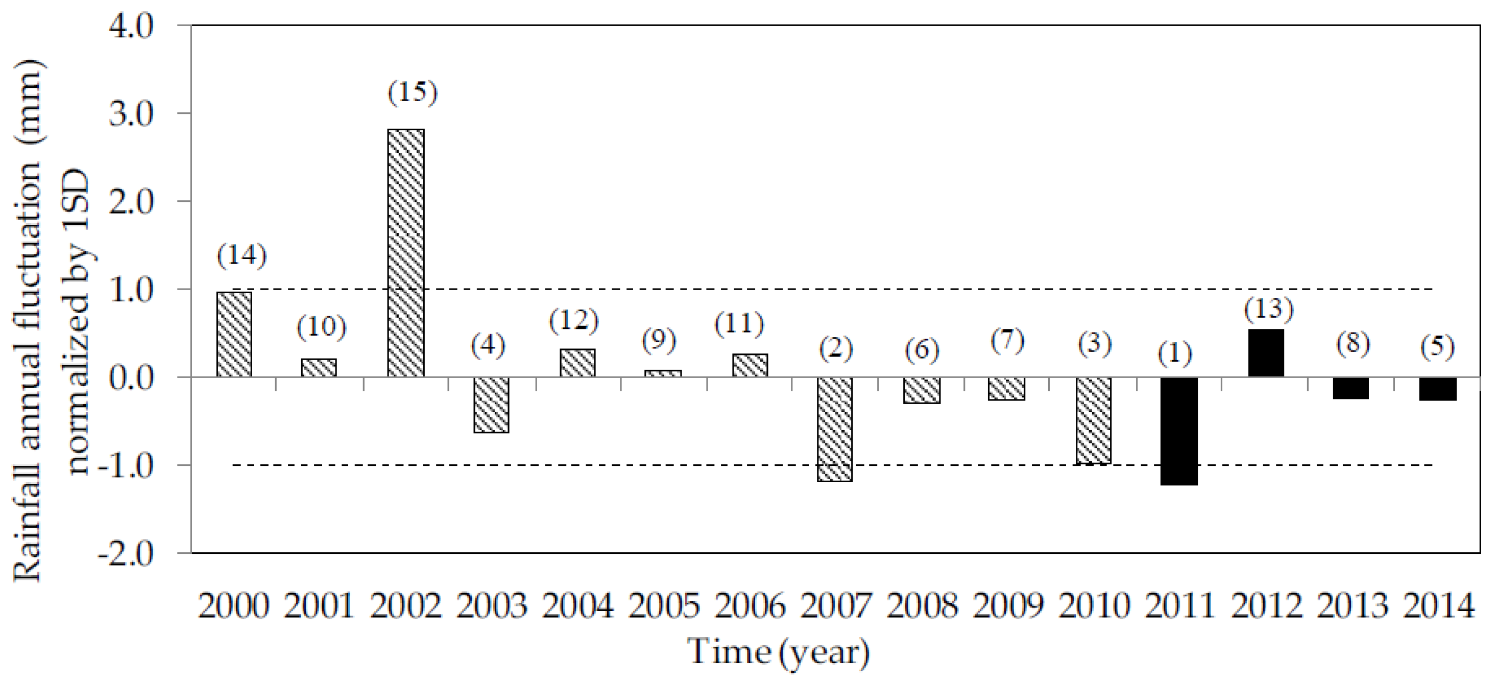
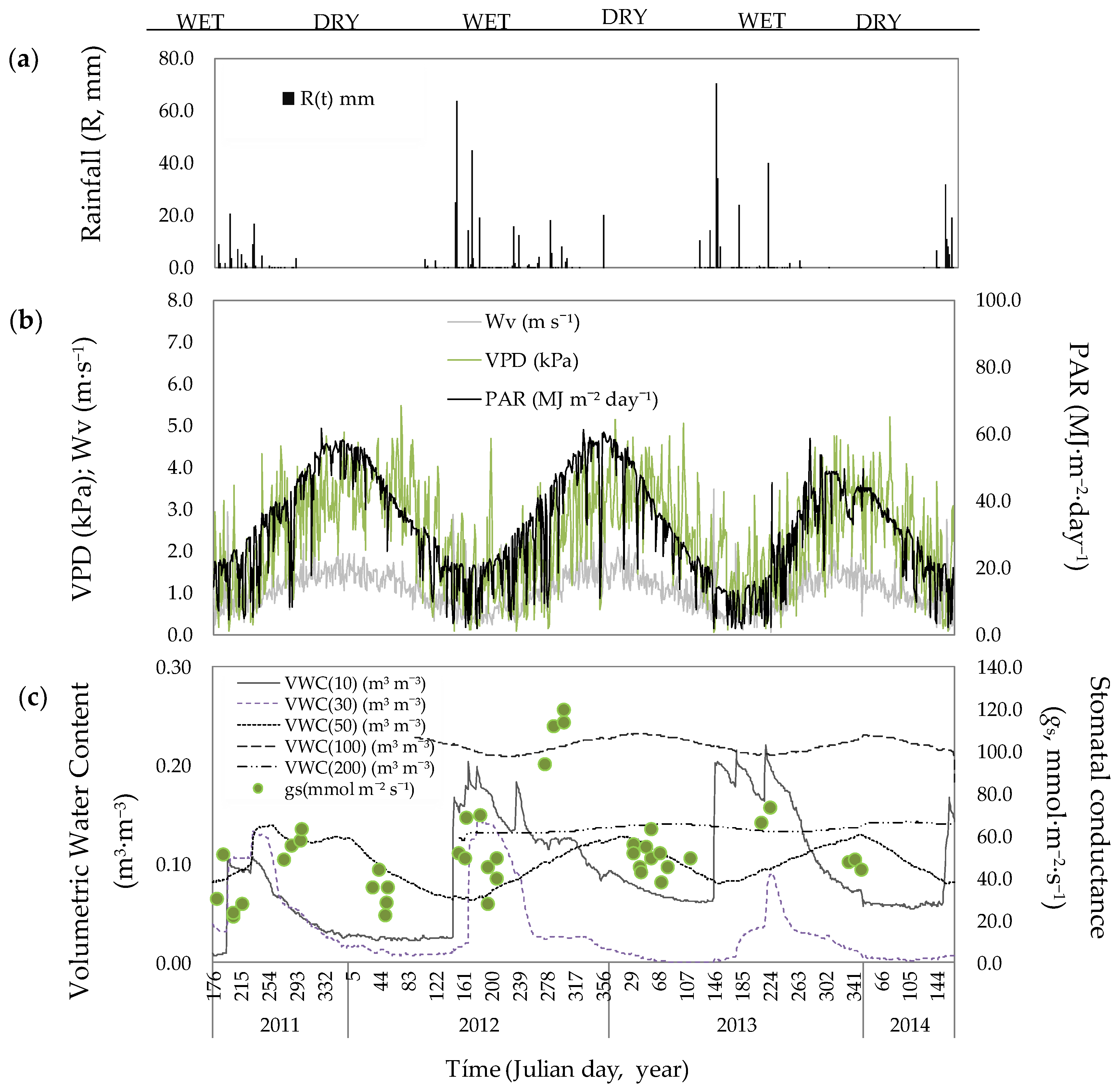
3.1. Environmental Conditions

Precipitation showed high interannual variation. For the period 2000–2014, years 2002, 2007, 2010 and 2011 were outside the band formed by the average ±1 standard deviation (Figure 3). Within this period, year 2011 was the driest, reaching only 50% of the average annual value, whereas 2012 the wettest, with 63.5 mm of surplus. Years 2013 and 2014 were below the average but within the expected variability for this period. At a monthly scale (Figure 4a), the rainfall events were concentrated in the wet season, between May and June.

Daily averages of wind velocity ($\mathrm{Wv}$), VPD, and PAR, show the typical pattern of a Mediterranean climate with a cold-wet followed by a hot-dry season (Figure 4b). Values of $\mathrm{Wv}$ were on average 0.3 m·s⁻¹ in the wet season and 2.1 m·s⁻¹ in the dry season. PAR values ranged from less than 14 MJ·m⁻²·day⁻¹ in the wet season to more than 50 MJ·m⁻²·day⁻¹ in the dry season. Maximum daily VPD values in the order of 5 kPa were recorded towards the end of the dry season (February–April), with daily minimums of 0.5 kPa during the wet season.

3.2. Soil Volumetric Water Content

According to

Table 1. Summary of relevant soil physical variables based on four soil pits. Average values ±1SD.

	Un	Soil Layer Depth (i) in cm
		i = 10	i = 30	i = 50	i = 100
Field capacity	% weight	40.8 ± 4.8	40.2 ± 4.3	41.6 ± 3.9	47.1 ± 4.5
Wilting point	% weight	24.4 ± 3.2	25.5 ± 3.5	26.6 ± 4.2	30.6 ± 4.6
Organic Matter	%	1.8 ± 1.2	2.5 ± 1.4	3.9 ± 2.3	2.5 ± 1.6
Bulk density	g·cm−3	1.19 ± 0.08	1.16 ± 0.06	1.08 ± 0.06	1.13 ± 0.05
Texture	Sand (%)	21 ± 6.4		10 ± 3.2
	Silt (%)	28 ± 4.2		20 ± 3.1
	Clay (%)	51 ± 8.7		70 ± 5.1
Total porosity	%	55 ± 5.3	51 ± 5.5	51 ± 4.5	50 ± 4.5

, the soil at the study site is relatively homogeneous. The textural class is a clay with about 51% clay, 28% silt and 21% sand for the soil depth 0–30 cm. At a greater soil depth (30–100 cm), clay was about 70%, silt 20% and sand 10%. Soil porosity was about 52% independent of soil depth. Bulk density was also relatively stable with soil depth at 1.08–1.19 g·cm⁻³. Soil organic matter varied considerably, ranging from 1.8% at 10 cm to 3.9% at 50%, without a clear pattern to decrease with soil depth. We observed the development of roots as deep as 100 cm with greater abundance at the 30–50 cm. This would explain the high values of organic matter at this soil depth. At approximately 180–200 cm, we observed a horizon composed of dense material, of fine compacted structure, and with low water permeability and root development. Field capacity (FC) and permanent wilting point (PWP) were about 41% and 25% at 0–30 cm on a gravimetric basis, respectively. At 100 cm, FC and PWP were about 47% and 31%, respectively, about 6% above the values recorded at 0–30 cm, probably associated with the greater proportion of clay at this soil depth. Santra et al. [44] developed pedotransfer functions for arid areas in India and the United States, allowing the estimation of field capacity (FC, % = 27.80 − 0.231 × Sand + 0.262 × Clay) and permanent wilting point (PWP, % = 10.06 – 0.0847 × Sand + 0.303 × Clay). For a clay texture (51% Clay, 28% Silt, 21% Sand) such as the one found at 0–30 cm in soil depth, the predicted FC and PWP based on Santra et al. [44] equations would be 0.36 and 0.23 g·g⁻¹, respectively, with maximum potential available soil water (ASW) of about 0.13 g·g⁻¹. At 100 cm (70% clay, 20% silt, 10% sand), FC, PWP and ASW using Santra et al. [44] equations would be 0.44, 0.30 and 0.14 g·g⁻¹, respectively. These values would be similar to the ones found in this study. For additional information see Table S1 in the Supplementary Material.

The rain events during the wet season of 2011, 2012 and 2013 did not raise the VWC to field capacity (Figure 4c). Moreover, the VWC of the dry season of 2011/2012 was lower compared to the dry seasons of 2012/2013 and 2013/2014, probably because 2011 was the driest year of the 2000–2014 period (see Figure 3). Across all dry seasons for the period under study, the VWC at 10 cm were about 40–50% of the PWP.

The temporal dynamics of VWC depend on soil depth. At 10 cm, the soil responded rapidly—in an hourly scale—to the occurrence of rainfall pulses. Once the wet season ended, usually by the end of September, the VWC quickly decreased below the PWP and remained at that level until the first rains occurred during the following wet season, at which time the VWC rapidly increased. At 30 cm, the VWC behaved similarly to that at 10 cm regarding its marked seasonality, although showing a temporal delay (lag-time) with respect to the rainfall pulses. Visible increases in VWC at 30 cm were brought about by large rainfall pulses (>30 mm) and with the delayed response. We observed that at the start of the wet season, the levels in soil water content for the first two years in the study period were under the estimated PWP for this depth.

It is worth noting that the temporal behavior of VWC at 50 cm exhibited an anticyclic trajectory with respect to the period in which the rainfalls are concentrated, with a longer lag-time compared to the 30 cm soil depth. Consequently, the maximum value was recorded during the early phase of the dry season (November–December) at about 0.14 to 0.16 m³·m⁻³ and a minimum during the wet season (May–July) of 0.06–0.07 m³·m⁻³.

In contrast to the soil layer above, the VWC at 100 and 200 cm, showed a quasi-stable behavior during the whole period under study. When we observed the temporal dynamic of VWC, we noted that these are lower than the estimated PWP (Permanent Wilting Point) for these soil depths. However, this VWC represents a water reserve for the plant below 1 m in soil depth. The almost null seasonal variation in water content observed at these depths, along with a semi-permeable layer preventing the flow of water to the lower layers, suggests that A. caven may have extensive water use at this depth, particularly during the dry season. It is worth noting that the PWP is calculated for a soil water potential of −15 MPa equivalent to the point where sunflower plants would die. However, tree species from semiarid environments are known to use water at VWC as low as 0.08 m³·m⁻³, which are clearly below the standard PWP from laboratory analysis or pedotransfer equations [44].

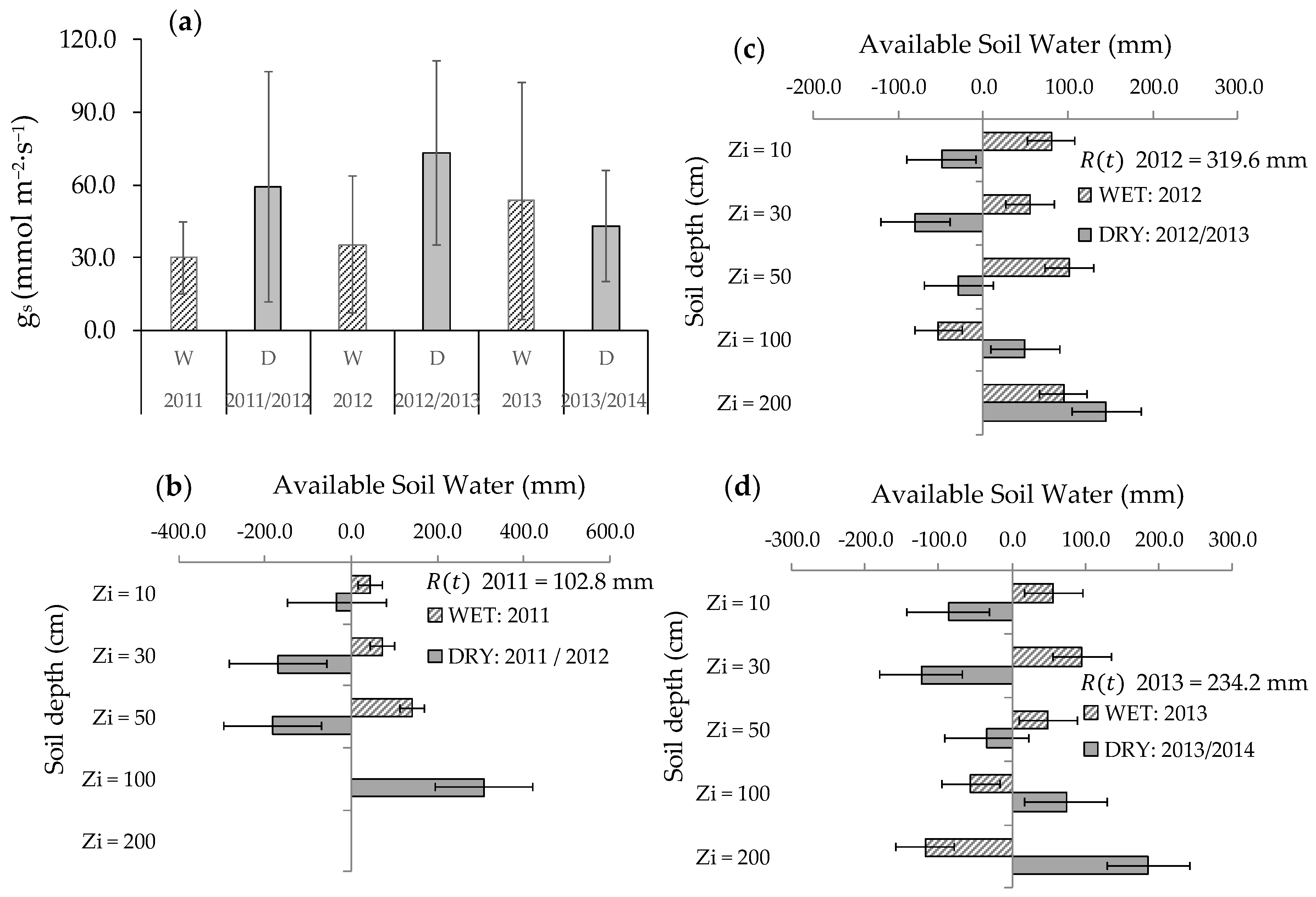
3.3. Stomatal Conductance and Vertical VWC Dynamics

Stomatal conductance ($g_s$) exhibited a clear seasonal behavior (Figure 5a). In the dry season, $g_s$ generally ranged from 40 to 60 mmol·m⁻²·s⁻¹, with a peak of 212 mmol·m⁻²·s⁻¹ recorded in October 2012, i.e., early in the dry season during the Austral spring. During the wet season, the $g_s$ values were much lower compared to the dry season, except for 2013, where this value surpassed 50 mmol·m⁻²·s⁻¹, becoming punctually 100 mmol·m⁻²·s⁻¹ towards the end of the wet season in the indicated year.

In Figure 5b–d, we show the vertical dynamics of VWC, considering the hydrological year for the southern hemisphere, within the root zone. We found positive and negative variations in available soil water (ASW) depending on soil depth. For example, rain events in the wet season of 2011 show positive variations at 10, 30 and 50 cm of soil depth, but negative variations in the 2011/2012 dry season, except to 100 cm. The same pattern for the other wet seasons under study was observed with positive variations in ASW down to 50 cm. Negative variations in ASW occurred consistently for the dry period under study, except in the deepest layers, at 100 and 200 cm, where variations were positive. This behavior is also consistent with the temporal dynamics observed in Figure 4c.

3.4. $g_s$ Responses to Environmental Conditions

Values of $g_s$ were weakly but significantly correlated to environmental variables. Atmospheric variables only explained about 5.4% of the $g_s$ variance when using the complete series (

Table 2. Results of the regression for $g_s$ as response variable, considering the complete series (CS) and the seasonal adjustment (K) of the atmospheric variables at the canopy level. ${\beta }_j$ indicates parameter regression; AtmV: atmospheric variables; $R^2,$ determination coefficient; MCE, modified coefficient of efficiency; MAE, mean absolute error. n corresponds to the sample size used in the analysis (329 records). D(t) and W(t), analysis corresponding to the dry and wet seasons, respectively.

	${\mathit{\beta }}_{\mathit{j}}$ (p < 0.05)
	$\mathbf{X}(\mathit{A}\mathit{t}\mathit{m}\mathit{V})(\mathbf{CS})$	$\mathbf{X}(\mathit{A}\mathit{t}\mathit{m}\mathit{V})(\mathbf{K})$
Variables	CS	D(t)	W(t)
${\mathit{T}}_{\mathit{leaf}}$	0.013	−0.364	0.319
${\mathit{W}}_{\mathit{v}}$	0.070	0.141	0.004
PAR	0.231	0.389	−0.101
VPD	0.026	0.001	0.132
Intercept	3.27	4.57	2.63
n	329	227	102
D-W	1.15	1.07	1.11
${\mathit{R}}^{\mathbf{2}}$(%)	5.4	17.8	12.3
		19.5
MCE	0.10	0.16
MAE	24.55	23.04

, Figure 6a). However, when partitioning the database for the wet and the dry seasons, the coefficient of determination increased to 17.8% for the dry season series and to 12.3% for the wet season series. Notably, in all cases, using either the complete series (CS) or the seasonal adjustment (K), the variables PAR and VPD, only in the wet season, made a significant contribution. When the simulated $g_s$ values for the complete series and with the seasonal adjustment were compared, we did not find significant differences in their medians (Kolmogorov−Smirnov test = 1.01, $p=0.18>0.05$) although their variances were different (F = 1.95; $p<0.05$). The same is true if each of the simulated series is compared with the observed $g_s$ values.

Precision and bias indicators in the models suggest that the seasonal adjustment provided a 14% improvement compared to the CS. The same occurs with MCE, being 0.16 for the seasonal adjustment (K) and 0.10 when using the complete series (CS).

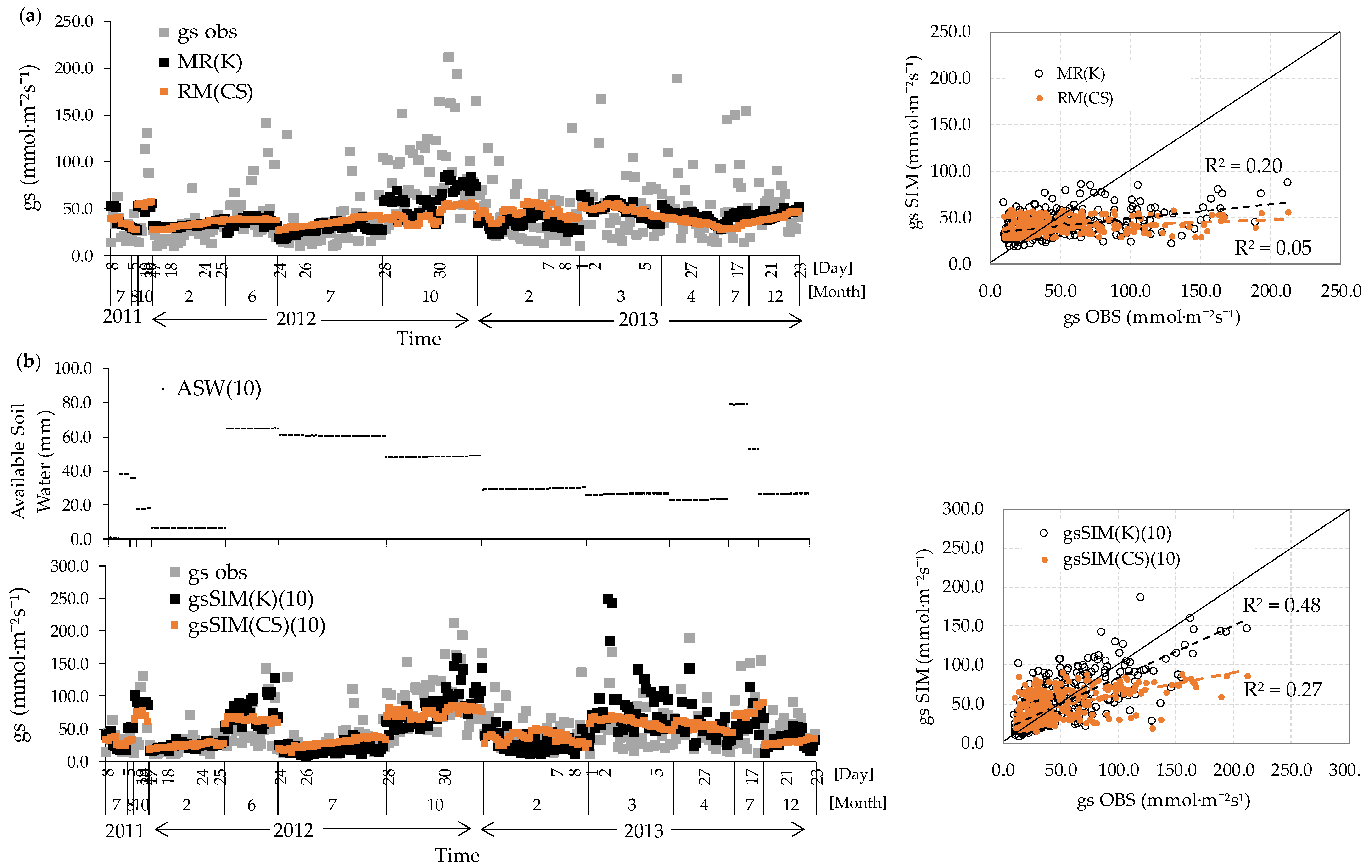
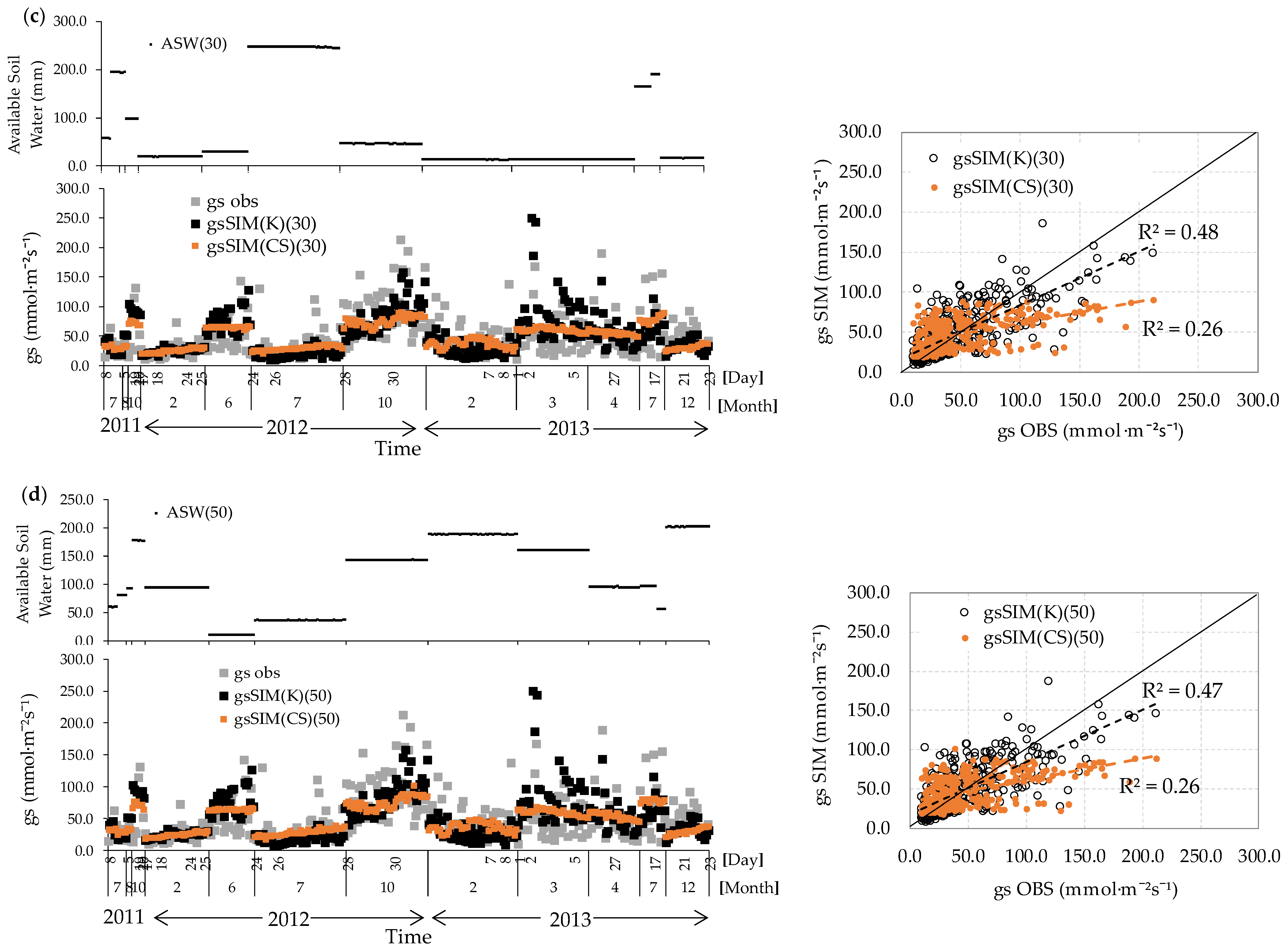
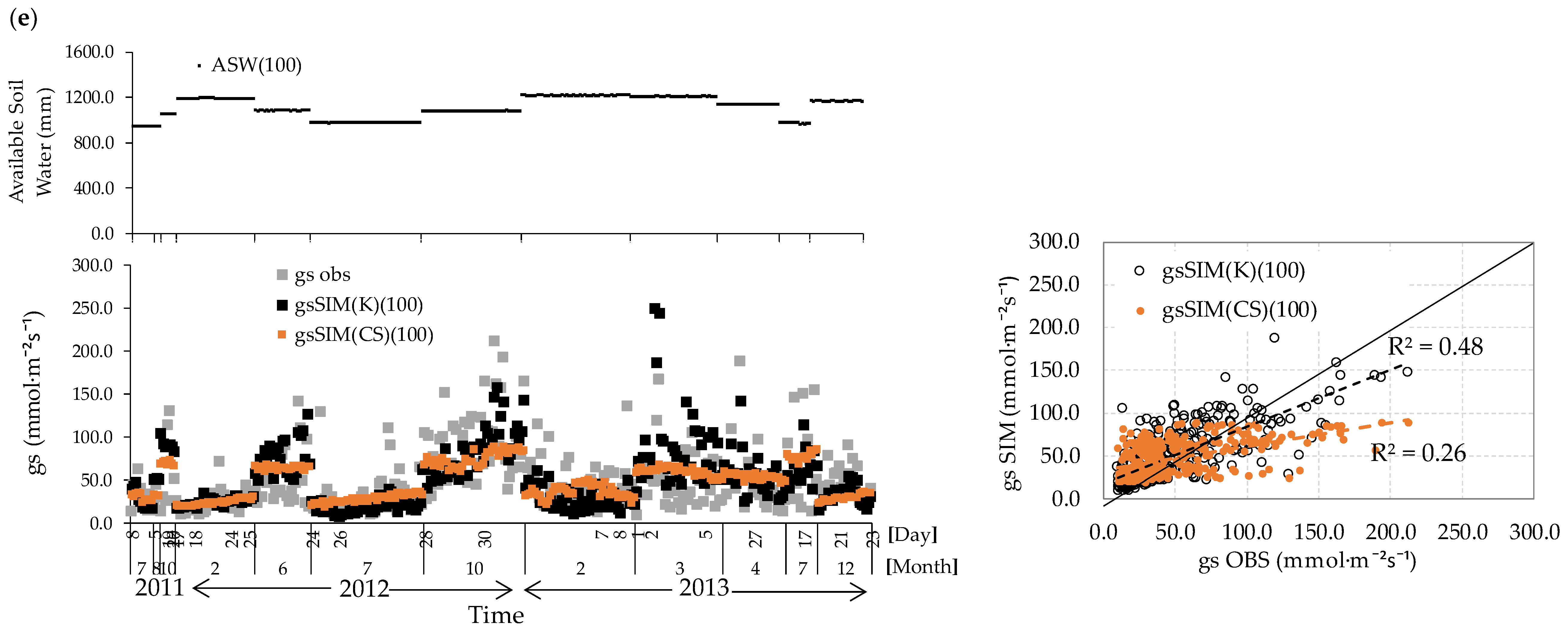
3.5. gs Responses Incorporating Volumetric Water Content

The residues ($N\left(t\right)$) generated from the Multiple Regression (MR) models were analyzed to identify an auto-regressive ($AR\left(f\right)$) structure in a dynamic regression (DR) context. Based on an AR model adjusted, we determinate a one significant dephasing ($f=1$ month) in the $g_s$ response regarding the VWC dynamics. This lag-time was also observed in its cross-correlations ($r_{xy}\left(f\right)$) functions, and clearly indicates an asynchrony relationship between VWC and $g_s$.

We also analyzed different configurations for the transference function (TF) model, which allowed us to determine that TF$(r=2,s=1,b=1)$ was statistically superior. With this TF(2,1,1) model (see

Table 3. Parameters and indicators for the dynamic regression (DR) analysis. (a) Estimation of the TF(2,1,1) coefficients with seasonal adjustment (K) and complete series (CS) incorporating the VWC records at different depths in the root zone. (b) Efficiency criteria of the $g_{sSIM}$ models obtained, where $R^2$ is the coefficient of determination; MCE, modified coefficient of efficiency; MAE, mean absolute error, calculated with respect to the observed $g_s$ values; $Z_i$, soil depth (in cm).

(a)	$\mathit{N}\left(\mathit{t}\right)\left(\mathbf{K}\right)=\mathbf{DR}(\mathit{REW}({\mathit{Z}}_{\mathit{i}}))$				$\mathit{N}\left(\mathit{t}\right)(\mathbf{CS})=\mathbf{DR}(\mathit{REW}({\mathit{Z}}_{\mathit{i}}))$
$\mathbf{FT}(\mathbf{211})$	$\mathit{i}=$10	$\mathit{i}=$30	$\mathit{i}=$50	$\mathit{i}=$100	$\mathit{i}=$10	$\mathit{i}=$30	$\mathit{i}=$50	$\mathit{i}=$100
${\delta }_1$	0.002	0.005	0.005	0.003	0.002	0.005	0.005	0.003
${\delta }_2$	−0.029	−0.028	−0.021	−0.027	−0.029	−0.028	−0.021	−0.027
${\varpi }_0$	0.038	−0.017	−0.001	0.029	0.038	−0.017	−0.001	0.029
${\varpi }_1$	−0.017	0.049	0.096	−0.027	−0.017	0.049	0.096	−0.027
(b)	${\mathit{g}}_{\mathit{sSIM}}\left(\mathit{t}\right)\left(\mathbf{K}\right)$				${\mathit{g}}_{\mathit{sSIM}}\left(\mathit{t}\right)\left(\mathbf{CS}\right)$
	$\mathit{i}=$10	$\mathit{i}=$30	$\mathit{i}=$50	$\mathit{i}=$100	$\mathit{i}=$10	$\mathit{i}=$30	$\mathit{i}=$50	$\mathit{i}=$100
MCE	0.49	0.48	0.49	0.49	0.44	0.44	0.45	0.44
MAE	13.96	14.27	14.05	14.16	15.33	15.36	15.22	15.34
R2	47.7%	47.9%	47.2%	47.6%	26.8%	26.2%	25.6%	26.0%

a), we characterized the residues $N\left(t\right)$ for each simulated series with seasonal adjustment (K), as well as the complete series (CS), and for each depth in the root zone. We generated new simulated series of $g_s$ values, whose behavior with respect to the series of observed values ($g_{sOBS}$) are presented in Figure 6.

In Table 3b, statistics of precision and bias are shown. In this regard, the MCE values are slightly better under a seasonal adjustment, although this difference was not significant. The same was observed with the absolute errors, where the differences in the MAE between the groups did not surpass 2 mmol·m⁻²·s⁻¹, which was inferior in all cases to the observed standard deviation (36.6 mmol·m⁻²·s⁻¹). Finally, the analysis considering seasonality shows $R^2$ values about 47%. In contrast, these $R^2$ are significantly superior ($t=$ 24.7; $p<0.05$) to those obtained in the models using the complete series that also integrates the VWC at different $Z_i$ ($g_{sSIM}\left(t\right)(\mathrm{CS})$).

Figure 6 shows that the adjustment improved significantly between the months of August and October, when the $g_s$ variability is maximal because the plant has started its annual production, i.e., new leaves and branches. Likewise, by incorporating the N(t) analysis, the model allows a better adjustment of the observed values during the middle of the dry season (February). However, there are not significant differences in their averages (ANOVA, $p>0.05$), and medians (Kruskal−Wallis test, kw = 13.56, $p=0.09>0.05$). In contrast, significant differences exist in their variances (Levene test: 4.87793; $p<0.05$), mainly because the performed adjustments do not represent the maximum punctual values observed during the study period.

3.6. Analysis of Remaining Errors Concerning the Explanatory Variables

Table 4. Main statistical values for remaining errors ($\mu$) according to multiple regression (MR) and dynamic regression (DR) analysis. Av: Average; SD: standard deviation; CV: coefficient of variation; Max: maximum value; Min: minimum value; K: seasonal; CS: complete series; $\mu \left(i\right)$, with i soil depths in cm (10, 30, 50 and 100).

	MR		DR Incorporating ${\mathit{Z}}_{\mathit{i}}$
			Seasonal (K)				Complete Serie (CS)
	µ(K)	µ(CS)	µ(10)	µ(30)	µ(50)	µ(100)	µ(10)	µ(30)	µ(50)	µ(100)
Av	1.21	1.24	1.10	1.10	1.11	1.10	1.09	1.08	1.09	1.08
SD	0.82	0.89	0.54	0.54	0.56	0.54	0.71	0.68	0.70	0.69
CV	0.68	0.72	0.49	0.49	0.51	0.49	0.65	0.63	0.65	0.64
Max	6.14	5.22	4.62	4.60	4.89	4.76	6.92	5.27	5.78	5.49
Min	0.15	0.19	0.13	0.13	0.13	0.13	0.16	0.16	0.16	0.17

shows the main statistical indicators regarding the remaining errors ($\mu =g_{sOBS}/g_{sSIM}$). As we can see, the average $\mu$ is $>1$ (underestimation) in the MR analysis, and in the DR analysis when incorporating the VWC at different soil depths. Also, we observed that when we included seasonality, the remaining errors were 21%. On the contrary, when incorporating REW($Z_i$) with the $N\left(t\right)$ analysis using DR, the remaining errors were between 8% and 11% with both the seasonal adjustment and the complete series. In all cases, the maximum values of remaining errors indicate large underestimations, between 2.5 and 4.4 times lower than the observed $g_s$ values.

When we incorporated REW, the $\mu$ obtained of seasonal adjustment (K) showed punctual maximum values (1 value in each case) between 4.6 and 4.8. On the contrary, in the CS analysis, we observed punctual maximums between 5.3 and 6.9, representing $<$ 1%.

The behavior of $\mu$ shows well-defined patterns depending upon the explanatory variable. For example, maximal errors are found when $T_{leaf}$ is approximately 25 °C. For PAR and VPD, the errors increased as each variable increased, although when $\mu$ is about 1.0, PAR is usually over 200 W·m⁻² and VPD > 1.0 kPa, which is consistent when considering that around such values, these variables are not a limiting factor in the response of the vegetation. Regarding VWC at different soil depths, the errors increase when REW(10) is found between 0.6 and 0.8 and when these reports are linked to specific moments after rainy days, during the wet season. The cases of REW(30) and REW(50) are similar; that is, the errors increase until reaching the maximum values associated with 0.2 and 0.5 and become smaller after the available water for the plant increases. Finally, the case of REW(100) was not significant.

4. Discussion

Our results show that the studied Acacia formation displays a typical temporal response when subjected to rapid interannual hydroclimatic changes, where the dry season is warm and lacks rainfall events. This condition characterizes what Vico et al. [1] define as seasonally dry ecosystems, which can also be observed in other countries of South America (e.g., campo limpo in Brazil and sabana de Acacia in Paraguay), Africa (e.g., foret Claire and miombo), Europe (e.g., maquis) and North America (e.g., chaparral and oak savannas in México and the United States), among others. According to Meza et al. [45], interannual variations are largely regulated by the El Niño-Southern Oscillation, which induces precipitation anomalies during the El Niño/La Niña phases.

Values of $g_s$ were significantly but weakly explained by atmospheric variables (about 5%), increasing to 19.5% when incorporating seasonal adjustments. In addition, interactions between the variables could be observed that could not be otherwise identified if only using the complete series. Specifically, the adjustment for the dry season ($n_D$ = 227 hourly records in the dry season) shows a better correlation ($r$) when compared with the wet season ($n_W$ = 102 hourly records in wet season), with values of 0.42 and 0.35, respectively. These values are consistent with those obtained by Rabb et al. [29] in an environment dominated by an Acacia caven savanna in central Chile. However, the authors classified the behavior of this species as isohydric, different from what our results suggest where a loose correlation with environmental variables is shown, suggesting an anisohydric behavior.

Although the relationship between $g_s$ and PAR and VPD are consistently reported in some studies [29,37], other variables, such as wind velocity ($W_v$) and leaf temperature, are rarely mentioned. VPD is a relevant variable in all the generated models based on atmospheric factors at the canopy level [45,46]. In our study, the incorporation of VPD was different from what was reported by Granier et al. [22] and Gao et al. [6], since we avoided the joint use of the records of temperature and relative humidity of the air, together with VPD, as this would induce circularity. The latter is consistent with Huang et al. [47] who reported that high VPD values (>2 kPa) exert a significant control on stomatal conductance and that when these values drop (<1 kPa), the $g_s$ increases with solar radiation.

In our study, the incorporation of VWC complemented the variables at the canopy level, and improved the temporal representation of stomatal conductance, mainly when considering a seasonal adjustment, similar to that reported by Oren et al. [17], Irvine et al. [18], and Huang et al. [47], among others. Likewise, significant VWC contribution was reported previously by Meza et al. [45], who, based on a study performed in a similar ecosystem in central Chile, determined that VWC was the main response activator of the ecosystem.

When we used the CS of observed hourly data (n = 329), the integration of REW contributed less than 5% in addition to the percentage of the unexplained variance. This contribution was mainly evident in the months of August and October, when we recorded an increment in plant activity, and to a lesser degree during the period without rainfall, between January and March. The latter period was also characterized by an increment in the levels of PAR and VPD, thus being considered as dominant variables. In this regard, Williams et al. [48], using a SVAT-type model (Soil-Vegetation-Atmosphere Transfer), determined that when the soil water content is low and VPD is high, the atmospheric variables predominate in the process of stomatal response.

Regarding the seasonal adjustment (K), the contribution of REW to $R^2$ is approximately between 27% and 28%, absolute errors between 23.04 and 24.55 mmol·m⁻²·s⁻¹, and MCE between 0.16 and 0.10, with no significant difference between soil depths. Our statistics were worse than those reported by Raab et al. [29], for Acacia caven in central Chile.

The generated results, both in the analysis of a CS, as well as in a seasonal adjustment (K), allows us to suggest that seasonality has a significant effect that is improved by the contribution of soil water. The latter is in line with the reports by Harris et al. [43], Oren and Pataki [49], and Oren et al. [17], who stated that the variability in stomatal response is affected by the variation in the water content in the root zone.

Due to high diurnal variability of $g_s$, the predictive performance of the model, relative to the variables considered in the analysis, was, in general, moderate. Given the configuration of the regression model $g_{sSIM}=e^{({\beta }_j\mathit{X})}$, we obtained simulated values below those observed. Regardless, both the observed and estimated values, in their average and maximums, are consistent with the reports by Xu and Baldocchi [50], Mediavilla and Escudero [51], Matsumoto et al. [37], Uddling et al. [52] and Raab et al. [29]. The implemented seasonal analysis, similar in scope to Matsumoto et al. [37] and Huang et al. [47], presented maximum values between 180 and 210 mmol·m⁻²·s⁻¹, for the phase with higher plant activity during an early stage of the dry season; that is, between October and November. Complementing these findings, we obtained values between 40 and 100 mmol·m⁻²·s⁻¹ at mid and late phases of the dry season (between February and March) that are similar to those values reported by Raab et al. [29]. Low VWC values in the root zone were notorious in the first 30 cm during the dry season.

The behavior of the residue error series ($\mu$) shows a similar pattern for CS and K. We observed a more pronounced subestimation for the atmospheric variables and, in general, a more stable behavior for VWC at different depths in the root zone. In all the analyzed cases, the $\mu$ values vary around 1.0, which shows that generally estimated values were unbiased.

Our results show that A. caven possesses a highly active radicular system in the first 100 cm of the soil showing evident adaptations to the soil hydric conditions, allowing the species to make extensive use of the water accumulated in the soil after rainfall events. According to Roman et al. [53], plant species growing under seasonal drought, like Acacia caven, could decrease leaf water potential during drought by sustaining relatively high $g_s$ and thus carbon assimilation, becoming more susceptible to hydraulic failure at midday. Considering our initial hypothesis, the temporal variability in stomatal conductance can be better explained if both the seasonality of the atmospheric variables and the vertical dynamics of the VWC are incorporated.

Finally, the limitations of the performed analyses must be considered. On one hand, this study is restricted to the observed values, and on the other, it is site-specific. The former has been partially overcome as we count with meteorological records for three contrasting conditions—one extremely dry year (2011), a humid year (2012), and two dry years (2013–2014)—which provides a wider range regarding the behavior of the environment under study. The second limitation is associated with the inherent restriction of regression analysis assessing correlation but not necessarily causality.

5. Conclusions

We have characterized the temporal dynamics of leaf stomatal conductance at a site scale in a savanna-like shrubland formation of Acacia caven in central Chile, considering the synchronic behavior of atmospheric variables and asynchrony in soil water availability at different depths in the roots zone. We found that:

(1)

A clear gain was achieved in the temporal representation of $g_s$ based on atmospheric variables at the level of the canopy when incorporating the VWC in the root zone.

(2)

The contribution of VWC at different depths in the root zone was relevant when performing an adjustment with the CS and seasonal adjustment. In the first case, VWC and not the atmospheric variables determined the seasonal fluctuation in the simulated series.

(3)

When we included seasonality in the adjustment of atmospheric variables, VWC was also a relevant variable.

(4)

No differentiated use of water within the root zone, but rather a constant activity of the radicular system, was observed as a whole in the capture of available water at 100 cm.

References

1. Vico, G.; Thompson, S.E.; Manzoni, S.; Molini, A.; Albertson, J.D.; Almeida-Cortez, J.S.; Fay, P.A.; Feng, X.; Guswa, A.J.; Liu, H.; et al. Climatic, ecophysiological, and phenological control son plant ecohydrological strategies in seasonally dry ecosystems. Ecohydrology 2015, 8, 660–681. [Google Scholar] [CrossRef]
2. Noy-Meir, I. Desert ecosystems: Environment and producers. Annu. Rev. Eco. Syst. 1973, 4, 25–51. [Google Scholar] [CrossRef]
3. Tietjen, B.; Zehe, E.; Jeltsch, F. Simulating plant water availability in dry lands under climate change: A generic model of two soil layer. Water Resour. Res. 2009, 45, W01418. [Google Scholar] [CrossRef]
4. Miranda, J.; Jorquera, M.J.; Pugnaire, F.I. Phenological and reproductive responses of a semiarid shrub to pulsed watering. Plant Ecol. 2014, 215, 769–777. [Google Scholar] [CrossRef]
5. Katul, G.; Ellsworth, D.; Lai, C.-T. Modelling assimilation and intercellular CO2 from measured conductance: A synthesis of approaches. Plant Cell Environ. 2000, 23, 1313–1328. [Google Scholar] [CrossRef]
6. Gao, Q.; Zhao, P.; Zeng, X.; Cai, X.; Shen, W. A model of stomatal conductance to quantify the relationship between leaf transpiration, microclimate and soil water stress. Plant Cell Environ. 2002, 25, 1373–1381. [Google Scholar] [CrossRef] [Green Version]
7. Arve, L.E.; Torre, S.; Olsen, J.E.; Tanino, K.K. Stomatal responses to drought stress and air humidity. In Abiotic Stress in Plants—Mechanisms and Adaptations; IntechOpen: London, UK, 2011. [Google Scholar] [CrossRef]
8. Schulze, E.D.; Kelliher, F.M.; Körner, C.; Lloyd, J.; Leuning, R. Relationships among maximum stomatal conductance, ecosystem surface conductance, carbon assimilation rate and plant nitrogen nutrition: A global ecology scaling exercise. Annu. Rev. Ecol. Syst. 1994, 25, 629–660. [Google Scholar] [CrossRef]
9. Ding, R.; Kang, S.; Du, T.; Hao, X.; Zhang, Y. Scaling up stomatal conductance from leaf to canopy using a dual-leaf model for estimating crop evapotranspiration. PLoS ONE 2014, 9, e95584. [Google Scholar] [CrossRef] [PubMed]
10. Damour, G.; Simonneau, T.; Cochard, H.; Urban, L. An overview of models of stomatal conductance at the leaf level. Plant Cell Environ. 2010, 33, 1419–1438. [Google Scholar] [CrossRef] [PubMed]
11. Cowan, I.R.; Farquhar, G.D. Stomatal function in relation to leaf metabolism and environment. Symp. Soc. Exp. Biol. 1977, 31, 471–505. [Google Scholar] [PubMed]
12. Law, B.E.; Falge, E.; Gu, L.; Baldocchi, D.D.; Bakwin, P.; Berbigier, P.; Davis, K.; Dolman, A.J.; Falk, M.; Fuentes, J.D.; et al. Environmental controls over carbon dioxide and water vapor exchange of terrestrial vegetation. Agric. For. Meteorol. 2002, 113, 97–120. [Google Scholar] [CrossRef] [Green Version]
13. Schulze, E.D.; Mooney, H.A.; Sala, O.E.; Jobbagy, E.; Buchmann, N.; Bauer, G.; Canadell, J.; Jackson, R.B.; Loreti, J.; Oesterheld, M.; et al. Rooting depth, water availability, and vegetation cover along an aridity gradient in Patagonia. Oecologia 1996, 108, 503–511. [Google Scholar] [CrossRef] [PubMed]
14. Zavala, M. Integration of drought tolerance mechanisms in Mediterranean sclerophylls: A functional interpretation of leaf gas exchange simulators. Ecol. Modell. 2004, 176, 211–226. [Google Scholar] [CrossRef]
15. Anderegg, W.R.L.; Wolf, A.; Arango-Velez, A.; Choat, B.; Chmura, D.J.; Jansen, S.; Kolb, T.; Li, S.; Meinzer, F.; Pita, P.; et al. Plant water potential improves prediction of empirical stomatal models. PLoS ONE 2017, 12, e0185481. [Google Scholar] [CrossRef] [PubMed]
16. Anav, A.; Proietti, C.; Menut, L.; Carnicelli, S.; De Marco, A.; Paoletti, E. Sensitivity of stomatal conductance to soil moisture: Implications for troposphere ozone. Atmos. Chem. Phys. 2018, 18, 5747–5763. [Google Scholar] [CrossRef]
17. Oren, R.; Ewers, B.E.; Todd, P.; Phillips, N.; Katul, G. Water balance delineates the soil layer in which moisture affects canopy conductance. Ecol. Appl. 1998, 8, 990–1002. [Google Scholar] [CrossRef]
18. Irvine, J.; Perks, M.P.; Magnani, F.; Grace, J. The response of Pinus sylvestris to drought: Stomatal control of transpiration and hydraulic conductance. Tree Physiol. 1998, 18, 393–402. [Google Scholar] [CrossRef] [PubMed]
19. Stewart, J.B. Modelling surface conductance of pine forest. Agric. For. Meteorol. 1988, 43, 19–35. [Google Scholar] [CrossRef]
20. Gu, D.; Wang, Q.; Otieno, D. Canopy transpiration and stomatal responses to prolonged drought by a dominant desert species in Central Asia. Water 2017, 9, 404. [Google Scholar] [CrossRef]
21. Emanuel, R.; D’Odorico, P.; Epstein, H. A dynamic soil water threshold for vegetation water stress derived from stomatal conductance models. Water Resour. Res. 2005, 43. [Google Scholar] [CrossRef]
22. Granier, A.; Bréda, N.; Biron, P.; Villete, S. A lumped water balance model to evaluate duration and intensity of drought constraints in forest stands. Ecol. Modell. 1999, 116, 269–283. [Google Scholar] [CrossRef]
23. Cudennec, C.; Leduc, C.; Koutsoyiannis, D. Dryland hydrology in Mediterranean regions—A review. Hydrol. Sci. J. 2007, 52, 1077–1087. [Google Scholar] [CrossRef]
24. Gerstmann, C.; Miranda, M.; Condal, A. Description of space-time variability of the potential productivity of Acacia caven espinales based on MODIS images and the Enhanced Vegetation Index (EVI). Cienc. Investig. Agrar. 2010, 37, 63–73. [Google Scholar] [CrossRef]
25. Ovalle, C.; Avendaño, J.; Aronson, J.; Del Pozo, A. Land occupation patterns and vegetation structure in the anthropogenic savannas (espinales) of central Chile. For. Ecol. Manag. 1996, 86, 129–139. [Google Scholar] [CrossRef]
26. Aronson, J.; Ovalle, C.; Aguilera, L.; Leon, P. Phenology of an ‘inmigrant’ savanna tree (Acacia caven, Legumoniosae) in the Mediterranean climate zone of Chile. J. Arid Environ. 1994, 27, 55–70. [Google Scholar] [CrossRef]
27. Schultz, J.J.; Cayuela, L.; Rey-Benayas, J.M.; Schröder, B. Factors influencing vegetation cover change in Mediterranean Central Chile (1975–2008). Appl. Veg. Sci. 2011, 14, 571–582. [Google Scholar] [CrossRef]
28. Van de Wouw, P.; Echeverria, C.; Rey-Benayas, J.M.; Holmgren, M. Persistent Acacia savannas replace Mediterranean sclerophyllous forests in South America. For. Ecol. Manag. 2011, 262, 1100–1108. [Google Scholar] [CrossRef]
29. Raab, N.; Meza, F.J.; Franck, N.; Bambach, N. Empirical stomatal conductance models revel that the isohydric behavior of an Acacia caven Mediterranean Savannah scales from leaf to ecosystem. Agric. For. Meteorol. 2013, 213, 203–216. [Google Scholar] [CrossRef]
30. Peel, M.C.; Finlayson, B.L.; McMahon, T.A. Updated world map of the Köppen-Geiger climate classification. Hydrol. Earth Syst. Sci. 2007, 11, 1633–1644. [Google Scholar] [CrossRef]
31. Sepulveda, M.; Bown, E.H.; Miranda, M.D.; Fernandez, B. Impact of rainfall frequency and intensity on inter- and intra-annual satellite-derived EVI vegetation productivity of an Acacia caven shrubland community in Central Chile. Plant Ecol. 2018. [Google Scholar] [CrossRef]
32. Allen, R.G.; Pruitt, W.O.; Raes, D.; Smith, M.; Pereira, L.S. Estimating evaporation from base soil and the crop coefficient for the initial period using common soils information. J. Irrig. Drain. Eng. 2005, 131, 14–23. [Google Scholar] [CrossRef]
33. Abtew, W.; Melesse, A.M. Evaporation and Evapotranspiration: Measurements and Estimations; Springer: Argovie, The Netherlands, 2013; ISBN 978-94-007-4737-1. [Google Scholar]
34. Blake, G.R. Bulk density. In Methods of Soil Analysis: Part 1, Physical and Mineralogical Properties, Including Statistics of Measurement and Sampling; Black, C.A., Evans, D.D., White, J.L., Ensminger, L.E., Clark, F.E., Eds.; American Society of Agronomy: Madison, WI, USA, 1965; pp. 374–390. [Google Scholar]
35. Johnson, M.-V.; Kiniry, J.; Burson, B. Ceptometer deployment method affects measurement of fraction of intercepted photosynthetically active radiation. Agron. J. 2010, 102, 1132–1137. [Google Scholar] [CrossRef]
36. Zuur, A.F.; Leno, E.N.; Elphick, C.S. A protocol for data exploration to avoid common statistical problems. Meth. Ecol. Evol. 2010, 1, 3–14. [Google Scholar] [CrossRef]
37. Matsumoto, K.; Ohta, T.; Tanaka, T. Dependence of stomatal conductance on leaf chlorophyll concentration and meteorological variables. Agric. For. Meteorol. 2005, 132, 44–57. [Google Scholar] [CrossRef]
38. Urban, J.; Ingwers, M.W.; McGuire, M.A.; Teskey, R.O. Increase in leaf temperature opens stomata and decouples net photosynthesis from stomatal conductance in Pinus taeda and Populus deltoids x nigra. J. Exp. Bot. 2017, 68, 1757–1767. [Google Scholar] [CrossRef] [PubMed]
39. Coleman, M.L.; Niemann, J.D. An evaluation of nonlinear methods for estimating catchment-scale soil moisture patterns based on topographic attributes. J. Hydroinf. 2012, 14, 800–814. [Google Scholar] [CrossRef] [Green Version]
40. Wooldridge, J.M. Introductory Econometrics: A Modern Approach, 5th International ed.; South-Western: Mason, OH, USA, 2013; pp. 409–415. [Google Scholar]
41. Bennett, N.D.; Croke, G.F.W.; Guariso, G.; Guillaume, J.H.A.; Hamilton, S.H.; Jakeman, A.J.; Marsili-Libelli, S.; Newham, L.T.H.; Norton, J.P.; Perrin, C.; et al. Characterizing performance of environmental models. Environ. Modell. Softw. 2013, 40, 1–20. [Google Scholar] [CrossRef]
42. Legates, D.R.; McCabe, G.J. Evaluating the use of “goodness-of-fit” measures in hydrologic and hydroclimatic model validation. Water Resour. Res. 1999, 35, 233–241. [Google Scholar] [CrossRef]
43. Harris, P.P.; Huntingford, C.; Cox, P.M.; Gash, J.H.C.; Malhi, Y. Effect of soil moisture on canopy conductance of Amazonian rainforest. Agric. For. Meteorol. 2004, 122, 215–227. [Google Scholar] [CrossRef]
44. Santra, P.; Kumar, M.; Kumawat, R.N.; Painuli, D.K.; Hati, K.M.; Heuvelink, G.B.M.; Batjes, N.H. Pedotransfer functions to estimate soil water content at field capacity and permanent wilting point in hot Arid Western India. J. Earth Syst. Sci. 2018, 127, 35. [Google Scholar] [CrossRef]
45. Meza, F.J.; Montes, C.; Bravo-Martinez, F.; Serrano-Ortiz, P.; Kowalski, A.S. Soil water content effects on net ecosystem CO2 exchange and actual evapotranspiration in a Mediterranean semiarid savanna of Central Chile. Sci. Rep. 2018, 8, 8570. [Google Scholar] [CrossRef] [PubMed]
46. Ou, X.; Gan, Y.; Chen, P.; Qiu, M.; Jiang, K.; Wang, G. Stomata prioritize their responses to multiple biotic and abiotic signal inputs. PLoS ONE 2014, 9, e101587. [Google Scholar] [CrossRef] [PubMed]
47. Huang, Y.; Li, X.; Zhang, Z.; He, C.; Zhao, P.; You, Y.; Mo, L. Seasonal changes in Cyclobalanopsis glauca transpiration and canopy stomatal conductance and their dependence on subterranean water and climatic factors in rocky karst terrain. J. Hydrol. 2011, 402, 135–143. [Google Scholar] [CrossRef]
48. Williams, M.; Malhi, Y.; Nobre, A.D.; Rastetter, E.B.; Grace, J.; Pereira, M.G.P. Seasonal variation in net carbon exchange and evapotranspiration in a Brazillian rain forest: A modelling analysis. Plant Cell Environ. 1998, 21, 953–968. [Google Scholar] [CrossRef]
49. Oren, R.; Pataki, D.E. Transpiration in response to variation in microclimate and soil moisture in southeastern deciduous forests. Oecologia 2001, 127, 549–559. [Google Scholar] [CrossRef] [PubMed]
50. Xu, L.; Baldocchi, D.D. Seasonal trends in photosynthetic parameters and stomatal conductance of blue oak (Quercus douglasii) under prolonged summer drought and high temperature. Tree Physiol. 2003, 23, 865–877. [Google Scholar] [CrossRef] [PubMed]
51. Mediavilla, S.; Escudero, A. Stomatal responses to drought of mature trees and seedlings of two co-ocurring Mediterranean oaks. For. Ecol. Manag. 2004, 187, 281–294. [Google Scholar] [CrossRef]
52. Uddling, J.; Teclaw, R.M.; Pregitzer, K.S.; Ellsworth, D.S. Leaf and canopy conductance in aspen and aspen-birch forests under free-air enrichment of carbon dioxide and ozone. Tree Physiol. 2009, 29, 1367–1380. [Google Scholar] [CrossRef] [PubMed] [Green Version]
53. Roman, D.T.; Novick, K.A.; Brzostek, E.R.; Dragoni, D.; Rahman, F.; Phillips, R.P. The role of isohydric and anisohydric species in determining ecosystem-scale to severe drought. Oecologia 2015, 179, 641–654. [Google Scholar] [CrossRef] [PubMed]
Figure 1. (a) Location of the study area (white square) in central Chile. The gray area indicates an estimation of the extension of the Acacia caven savanna [24,25,26]. (b) The open circle indicates the location of the weather station (WS) and data loggers (DL) within the watershed. (c) Photograph of the Acacia caven savanna showing the enclosure within which the weather station (WS) and data logger (DL) were located.
Water 10 01534 g001
Figure 2. (a) Instrument set-up to measure atmospheric variables and soil volumetric water content at different soil depths. (b) A R indicates the area within which soil sensors were installed.
Water 10 01534 g002
Figure 3. Normalized annual precipitation for the period 2000–2014. Dark bars indicate the study period. The years are ranked from the driest to the rainiest in parentheses. Dashed lines represent ±1SD.
Water 10 01534 g003
Figure 4. (a) Rainfall (R, mm); (b) atmospheric variables (n = 1042 days): wind velocity ( W v , m·s−1); vapor pressure deficit (VPD, kPa) and photosynthetically active radiation (PAR, W·m−2); (c) daily average (n = 1042 days) for VWC (m3·m−3) at different soil depths (cm): 10, 30, 50, 100 and 200 cm, and leaf stomatal conductance daily average (mmol·m2·s−1) for n = 42 days with records. Julian day is shown in the x-axis considering day 1 being January 1st of every year.
Water 10 01534 g004
Figure 5. (a) Leaf stomatal conductance ( g s ) and (bd) vertical dynamics of available soil water (ASW) content for each soil depth (ASW = ( V W C i V W C P W P × Z i ) (mm)) based on hourly ASW total values ±1SD. Balance for the hydrological year was performed considering the period between March and April. Positive values represent “recharge” or “input” of water to the layer i, whereas negative values indicate an “output”. R ( t ) indicates total annual rainfall (mm).
Water 10 01534 g005
Figure 6. Behavior of the hourly average series for observed (OBS) and simulated (SIM) g s over 42 d with records while considering the seasonal adjustment (K) and the complete series (CS) of the atmospheric variables (a) and then for each one (be), incorporating the analysis of residues ( N ( t ) ) in function of the dynamic regression using REW( Z i ), where Z i is the depth in the soil at 10, 30, 50, and 100 cm within the root zone. ASW = ( V W C i V W C P W P ) × Z i , where Z i is the vertical length of the soil horizon. The x-axes indicate time in days, month and year.
Water 10 01534 g006aWater 10 01534 g006bWater 10 01534 g006c