Numerical and Experimental Comparative Study on the Flow-Induced Vibration of a Plane Gate

1
State Key Laboratory of Hydraulics and Mountain River Engineering, Sichuan University, Chengdu 610065, China
2
Faculty of Electrical Power Engineering, Kunming University of Science and Technology, Kunming 650500, China
*
Author to whom correspondence should be addressed.
Water 2018, 10(11), 1551; https://doi.org/10.3390/w10111551
Submission received: 13 September 2018
/
Revised: 26 October 2018
/
Accepted: 29 October 2018
/
Published: 31 October 2018
(This article belongs to the Special Issue Advances in Hydraulics and Hydroinformatics)
Abstract
:A numerical method is applied here to simulate the unstable flow and the vibration of a plane gate. A combination of the large eddy simulation (LES) method and the volume of fluid (VOF) model is used to predict the three-dimensional flow field in the vicinity of a plane gate with submerged discharge. The water surface profile, the streamline diagrams, the distribution of turbulent kinetic energy, the power spectrum density curve of the fluctuating pressure coefficient at typical points underneath the gate, and the complete vortex distribution around the gate are obtained by LES-VOF numerical calculation. The vibration parameters of the gate are calculated by the fluid-structure coupling interface transferring the hydrodynamic load. A simultaneous sampling experiment is performed to verify the validity of the algorithm. The calculated results are then compared with experimental data. The difference between the two is acceptable and the conclusions are consistent. In addition, the influence of the vortex in the slot on the flow field and the vibration of the gate are investigated. It is feasible to replace the experiment with the fluid-structure coupling computational method, which is useful for studying the flow-induced vibration mechanism of plane gates.
1. Introduction
With the wide application of a high head gate in hydraulic engineering, the vibration problem of the plane gate is increasingly prominent. Essentially, the flow-induced vibration of the plane gate is a complex fluid-structure interaction phenomenon. The time varying hydrodynamic load that is caused by the unstable flow around the gate is the main excitation source. The coexistence of the vortices at the gate’s bottom edge, in the gate slot and in the gate downstream, further complicates the flow structure of the sluice flow. However, it is difficult to capture these vortices simultaneously and to catch the comprehensive information of the vortex-induced vibration by using an experimental approach. Researchers, such as Hardwick [1], Kolkman [2], Jongeling [3], and Ishii [4], have been making efforts to explore the mechanism of gate vibration. Hardwick conducted a model test investigation on the plane gate vibration. It is believed that this nonlinear vertical vibration response is caused by the resonance between the fluid shear force acting at the bottom edge of the gate and the gate. Kolkman et al. believed that the flow fluctuation and the variation of the pressure due to the inertia effect of sluice flow might be the main reason for the vertical vibration of the gate. Jongeling proved that the streamwise vibration of the gate is induced by the instability of the bottom edge shear layer. Ishii considered that the vortices at the bottom edge of the gate and the interaction with the structure lead to the streamwise vibration of the gate. These research results are mostly limited to the qualitative description of the physical process of the gate vibration, and tend to separate the vertical vibration and the streamwise flow vibration. Therefore, it is especially important to analyze the vibration of the gate combining the vertical and the streamwise vibration. Simultaneously, these researches mainly focus on investigating the vibration mechanism that resulted from the vortex at the bottom edge of the gate.
With the rapid development of computational fluid dynamics (CFD) and computer technology, the accuracy of numerical calculation of flow field and the complexity of solving problems have been greatly improved, and it has been possible to numerically simulate the sluice flow in some extent. The method adopted is mainly based on the finite volume scheme. The SIMPLE series algorithm is used in the calculation of pressure field and velocity field. When dealing with turbulence problems, the turbulence model is employed to solve the Reynolds time-averaged Navier-Stokes equation. Pani et al. [5] used a finite element technique to investigate the fluid-structure interaction effect on the hydrodynamic pressure. Erdbrink et al. [6] also assessed the local velocities and pressures of the two-dimensional field by using the finite element method. Liu et al. [7] adopted the two-dimensional (2-D) mathematical model of Reynolds-averaged equations to study the turbulent flow behind a sluice gate. Kostecki [8,9,10] predicted the two-dimensional flow field in the vicinity of an underflow vertical lift gate by using a combinative numerical model of the vortex method and the boundary element method. Kazemzadeh [11] applied the smoothed fixed grid finite element method to simulate free surface flow in gated tunnels. In recent years, some novel computational methods and models have been developed. For example, Zhu et al. [12,13] proposed a new slip model, which was used in the study of lid-driven cavity flows in both continuum and transition flow regimes. However, there is still a lack of theories and methods to analyze effectively and deal with the complex vibration phenomenon of plane gates.
The development of parallel algorithms and supercomputers has strongly promoted the progress of direct numerical simulation (DNS) and large eddy simulation (LES) methods. Analyzing the pressure pulsation of turbulent flow using LES method has received more and more attention. However, the application of CFD technology, especially simulating pressure pulsation, in the sluice flow is still preliminary.
Different from the arc gate, the side walls of a plane gate have the gate slots that are used for the lifting movement of gate. In the case of the submerged sluice flow, the random movement of multiple vortices behind the gate, in the gate slot and at the gate’s bottom edge will aggravate the pulsation of velocity and the pressure. When water flow crosses the slot, such as that which exists in the hydraulic plane gate, the vortices in the slot will interact with the separated flow near the downstream corner of the slot due to local boundary mutation in the slot area, which can easily lead to flow cavitation and even endanger the safe operation of hydraulic projects [14]. The vortex-induced vibration of a blunt body or other solid boundary caused by vortex shedding has been studied most [15,16,17,18], while studies of the gate vibration induced by the vortex in the gate slot has been reported rarely.
Based on the theory of fluid-structure interaction, the present investigation studies the characteristics of the flow-induced vibration of the hydraulic plane gate with a submerged discharge. The three-dimensional numerical simulation method with a large eddy simulation turbulence model can obtain a complete flow structure, including a funnel vortex in the slot. The vibration parameters of the gate are acquired by the fluid-structure coupling interface transferring the hydrodynamic load. The fluid-structure coupling method is validated by the experimental evidence.
2. Computational Modeling
2.1. Turbulence Model
The large eddy simulation (LES) method uses instantaneous flow control equations to directly simulate the large scale vortex in a turbulent flow field. After processing by using the filtering function, the instantaneous Navier-Stokes equation and continuity equation of control fluid flow become:
where i, j = 1, 2, 3; is the specific mass; is the dynamic viscosity; is
the mass force; and,
and are the filtered pressure and velocity components, respectively. are the components of the sub grid scale (SGS) stress tensor representing the effect of the small scale motion on the large scale motion. According to the basic SGS model, Smagorinsky [19] assumes the SGS stress in the following form:
The Smagorinsky-Lilly model is used in this paper. In the Smagorinsky-Lilly [20] model, the eddy-viscosity is modeled by:
where , , Cs is the Smagorinsky constant; and, Δ is the local grid scale, which is computed according to the volume of the computational cell using Δ = V1/3.
It is more difficult to simulate the free surface accurately, and the volume of fluid (VOF) method is more advantageous to track the complex free surface in the multiphase flow models. Due to the downstream flow directly in contact with the atmosphere, the VOF model is used to track the air-water surface in the present investigation.
The tracking of the interface between the phases is accomplished by solving the continuity equation of the volume fraction of one or more phases. The volume fraction of water is a function of time and space, so the VOF model must be solved by transient. Assuming that αw denotes the volume fraction for water phase, αw = 0 indicates the exclusion of the water phase in the region, αw = 1 indicates that the region is full of water phase, and 0 < αw < 1 indicates the interface for water phase and other phases.
The tracking equations of the interface are as follows:
2.2. Structural Model
The gate structure is assumed to consist of linear elastic small deformation material, which is made of organic glass. Under the Lagrangian system, structural vibration control equations with a small deformation assumption are as follows:
The F, E, and J are defined as:
where is the density of structure, is the vibration displacement, is Cauchy’s stress tensor of the gate structure, and are the constants of the gate material, is material elastic modulus, and is Poisson’s ratio.
For complete fluid and structure coupling, the geometry coordination condition and the force equilibrium condition on the fluid-structure coupling interface should be satisfied.
The geometry coordination condition on the fluid-structure coupling interface is:
The force equilibrium condition on the fluid-structure coupling surface is:
where is the normal unit vector on the fluid-structure interface, is
the fluid region, and is the structure region. Due to the water flow effect, the gate structure contacting with the fluid vibrates, which leads to flow field changes. The changing flow field acts on the gate structure again, which forms fluid-structure interaction problems.
2.3. Meshing and Numerical Approach
The direction of flow is the x direction, the depth direction of flow is the y direction, and the direction across the flume is the z direction. Submerged discharge occurs downstream of the gate. The flow inlet is the speed boundary, and the flow outlet is the pressure boundary converted by the head. The top of the downstream flow is the air boundary, and the relative pressure is zero. The flume bottom and the sidewalls are no-slip solid boundary conditions, and the given normal velocity is zero. The method of the wall function is used for processing the near-wall viscous sublayer.
Due to the symmetry of the gate and the flume, half the model is selected to be meshed to reduce the calculating work. In this paper, the cases of the calculation are shown in Table 1, where e is the opening of the gate and H is the upstream water head. The underflow ratio U, is used to access the characteristics of the gate vibration caused by the submerged flow. Comprehensively considering the upstream and the downstream water head, underflow ratio U is defined, as follows:
where
is the downstream water depth, is the contraction section depth, is the conjugate water depth of the contraction section, and is the total head.
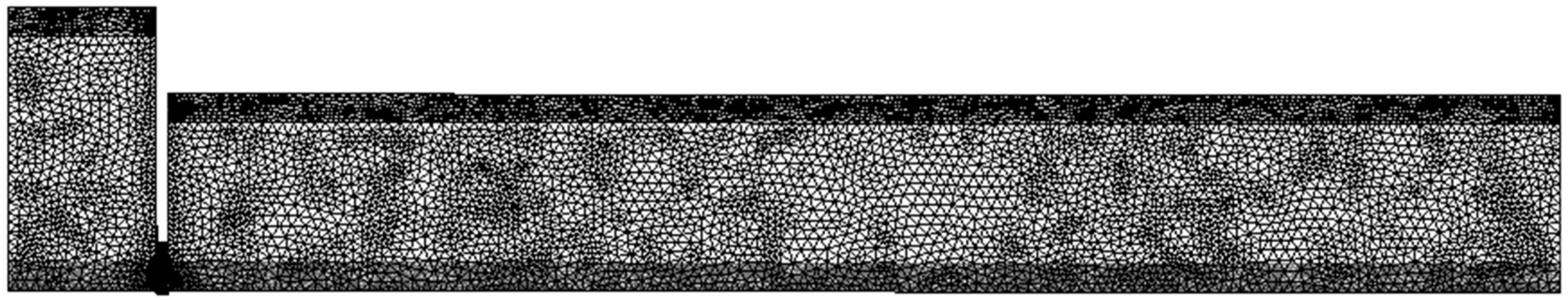
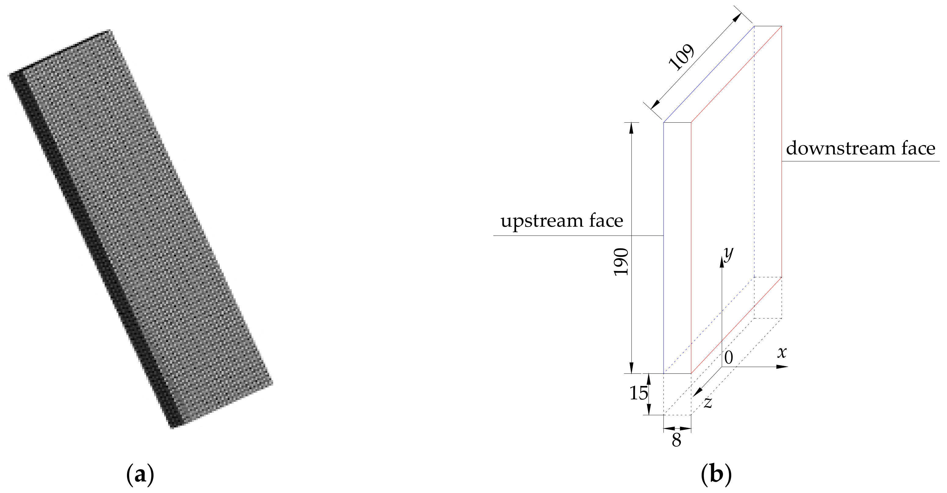
For U = 0.059, the half grid of fluid with tetrahedral mesh has 252,758 units and a total of 49,112 nodes (Figure 1). The time step length of unsteady flow is 0.001 s, and the maximum number of iterations of each step is 20 times. At the same time, the numerical simulation of turbulent flow under the unslotted condition is carried out to calculate the vortex effect of the gate slot. The half grid of the plane gate is shown in Figure 2a, and the size of the plane gate is shown in Figure 2b.
The ANSYS Worckbench17.0 is used to solve the system of dependent variables. After constructing a three-dimensional fluid-structure coupling model, the flow field in the vicinity of the lift gate with a submerged discharge condition is simulated by the finite volume method. A combination of the k − 𝜀 double-equation turbulence model and the VOF model of the multiphase flow is used to calculate the flow field before 10.5 s. With the result as the initial conditions of the Smagorinsky-Lilly subgrid model and the LES method after 10.5 s, the VOF model is still adopted to determine of the water-air interface. Velocity pressure coupling by the PISO algorithm and the momentum equation in discrete form by the second-order windward scheme are used to obtain the hydrodynamic pressure distribution that acts on the gate surface. Under the action of the surface pressure load, the vibration response of the gate structure is analyzed by the finite element method. To analyze the calculation results visually, the magnitude and the materials of the calculation model are consistent with the synchronous experiment model. The density, elastic modulus, and the Poisson’s ratio of the gate material are 1400 kg/m3, 3 × 10⁹ N/m2, and 0.4, respectively. Constraints are imposed on the top and sides of the gate. The width-to-depth ratio of the gate slot is 1.78.
3. The Results of Numerical Simulation
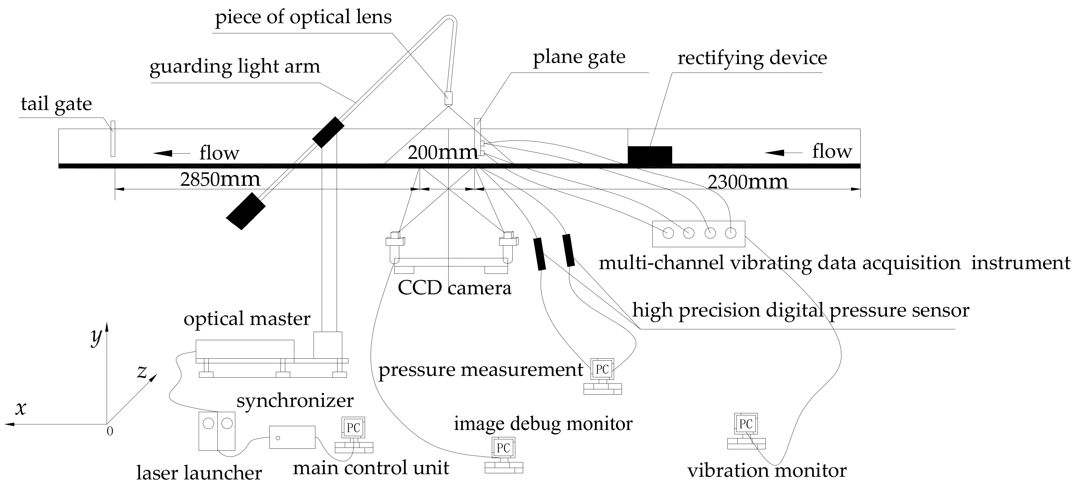
To verify the validity of the numerical simulation method, the numerical results are compared with the experimental data. The flow field behind the plane gate with submerged discharge, the hydrodynamic pressure process at typical points underneath the gate and the vibration parameters of the gate are acquired by the combination experiment [21] of three-dimensional particle image velocimetry (3D-PIV) made by TSI Company, the digital pressure sensor with high precision and the multichannel vibrating data acquisition system made by Lance Measurement Technologies Company, respectively.
The PIV test uses the Insight3G software to start the laser, and simultaneously captures the flow field particle images with two PIV-specific cross-frame CCD cameras. The autocorrelation or cross-correlation principle is used to extract the image of flow characteristics. Finally vector diagram of transient flow velocity in the measured range is obtained by professional post-processing software, such as Tecplot and Matlab. The maximum emission frequency of the laser is set to 14.5 Hz. In this test, a certain concentration of SiO2 is selected as the tracer particle, and the particle size is 10–15 μm. The three-axis accelerometer is directly attached to the upstream surface of the gate. The accuracy of the pressure sensor and accelerometer both are ±0.1%FS, and the sampling interval of the pulsating pressure and the vibration displacement are 0.01 s and 0.001 s, respectively. Three instruments are tested simultaneously.
The size of the organic glass flume is 4880 mm × 100 mm × 190 mm, and the length behind the plane gate is approximately 3000 mm. The calculations and the experimental cases are consistent with each other. The general arrangement of the experiment is shown in Figure 3.
3.1. Flow Field Distribution
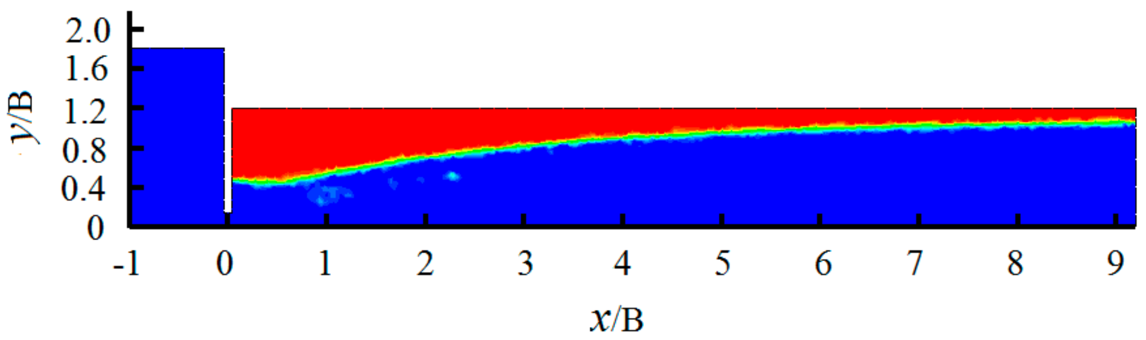
The calculation length after the lift gate is 920 mm and width B of the flume is 100 mm. The computation results of the time-averaged surface profiles with the whole flow passage of the modeling after the gate in U = 0.059 are shown in Figure 4. Blue represents the water phase and red represents the gas phase.
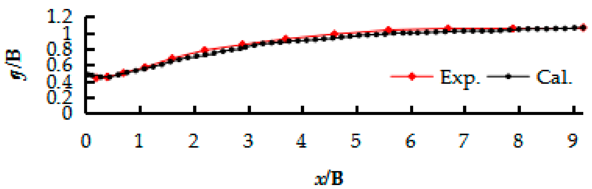
Figure 5 shows the time-averaged flow profile comparison behind the gate of section z = 0 mm for the calculation and experiment of U = 0.059. The maximum and minimum of relative difference of the height between the calculation and the test values of the flow profile are 4.8% and 0.16%, respectively, which shows that the VOF method can simulate the water-air interface well.
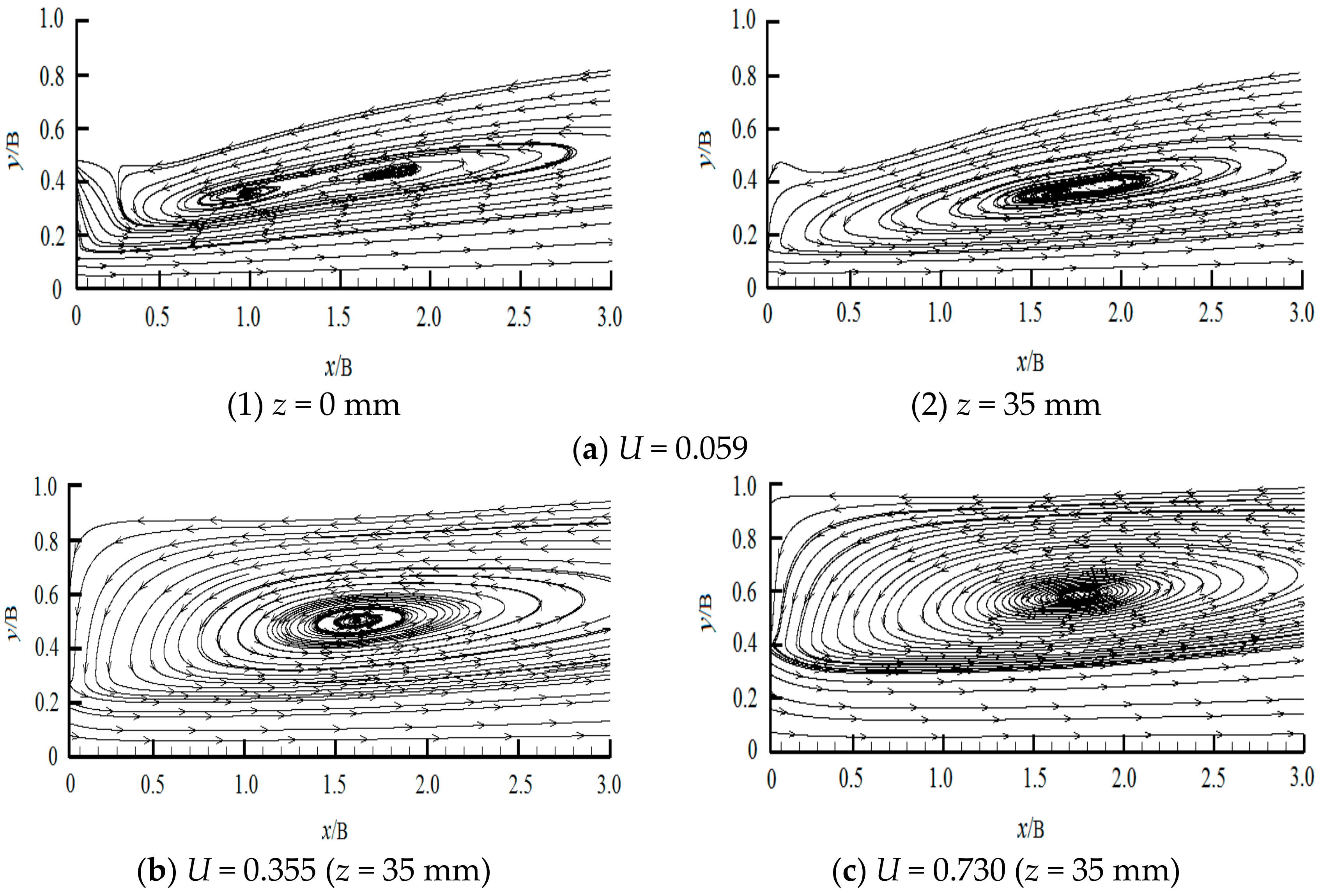
The calculational time-averaged streamlines on sections z = 0 mm and z = 35 mm in different cases are presented in Figure 6. According to (a), (b), and (c) in Figure 6, there is only a vortex on section z = 35 mm in the time-averaged flow field behind the plane gate in the x direction, but there are two vortices on section z = 0 mm that are within the 300 mm range. At different sections in the same case, the vertical distances of the vortex center from the x-axis are approximately the same. With the e/H increasing, the vertical distance of the vortex center from the x-axis increases gradually.
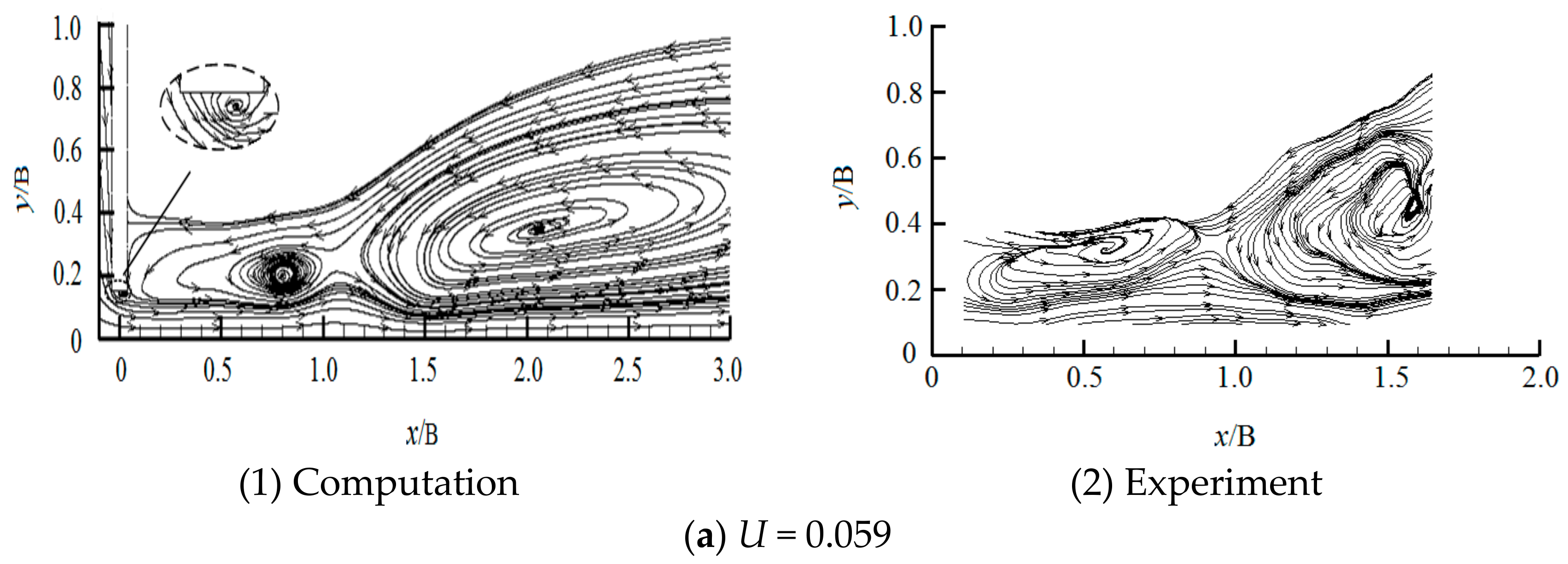
The size of the PIV calibration target is 200 mm × 200 mm. Due to the size limitation, it is impossible to test the vortices in the slot and at the bottom edge of the gate by PIV, so the computational results of only the vortices behind the gate are compared carefully with those of the three-dimensional PIV test. Both the simulated and the experimental velocity vector diagrams are achieved at 20.6 s.
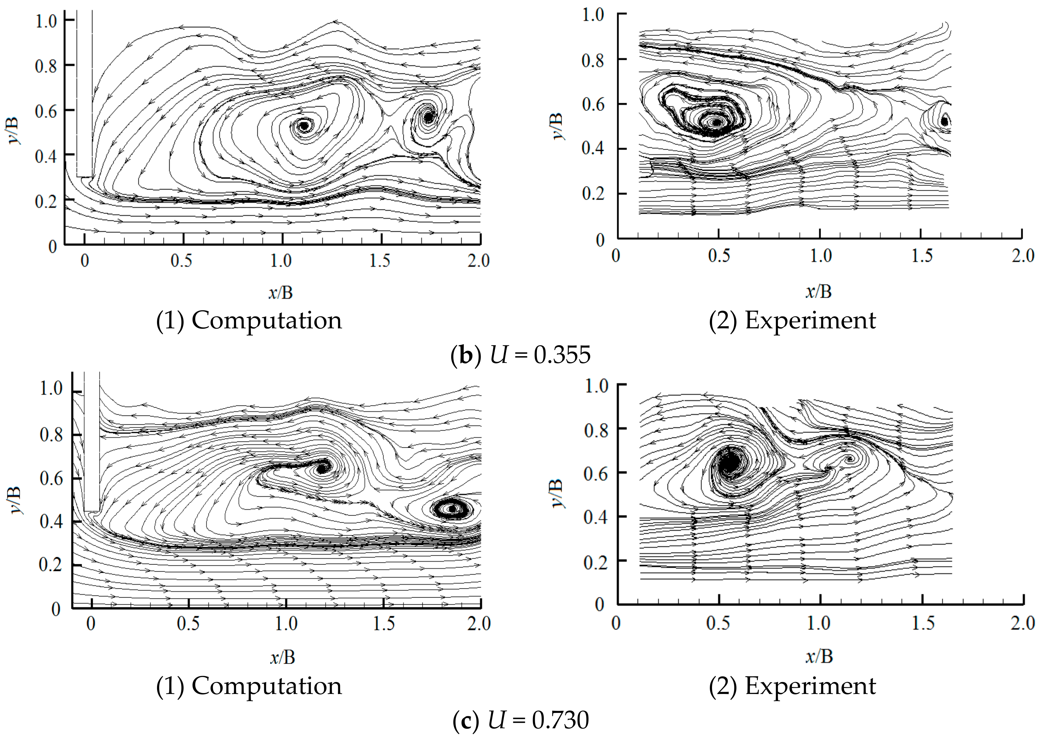
Figure 7 shows the instantaneous streamlines behind the gate on the same section z = 0 mm for the calculation and the experiment. The numerical simulation can make up for the drawback of losing the velocity vector by 3D-PIV positioning. When compared with the experimental results, the vortex center, which is closest to the gate obtained by the simulation, is lower in the y direction under U = 0.059, but this distance is basically same for the other two cases. On the whole, the numerical simulation still obtained the most ideal vortex information.
It can be seen from the instantaneous streamlines in Figure 7a–c that there are the same number of vortexes on section z = 0 mm between the computation and the experiment. Under U = 0.059, the numerical simulation captures the phenomenon of the vortex detachment from the gate’s bottom edge, but there is no such phenomenon when U = 0.355 or U = 0.730. Therefore, when the e/H and U reach a certain extent, the vortex shedding phenomenon can be generated from the bottom edge of the gate.
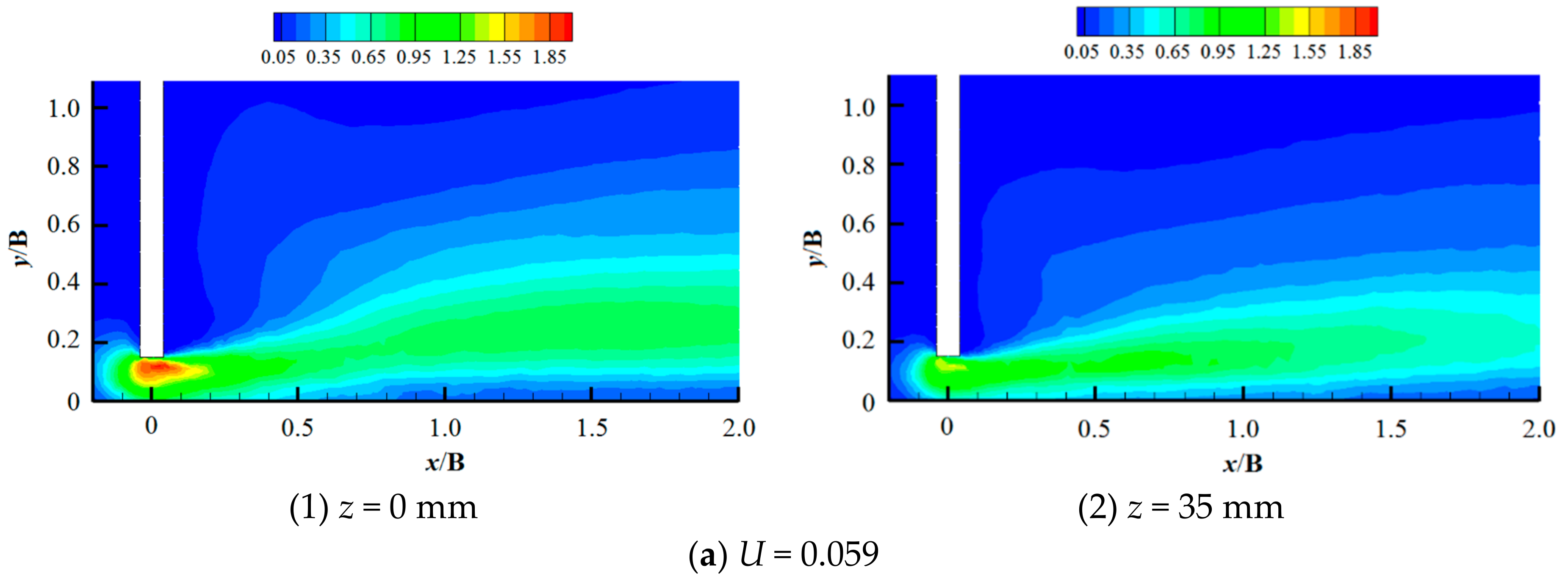
Normalizing the turbulent kinetic energy by the square of the mean flow velocity of the gate downstream section, Figure 8 presents the computational normalized turbulent kinetic energy distribution on section z = 0 mm and section z = 35 mm. Turbulent kinetic energy under the gate on section z = 0 mm is higher than the value on section z = 35 mm. The different magnitude of turbulent kinetic energy is one of the significant factors affecting the gate vibration extremum. The experiment proved that the extremum of vibration displacement on section z = 0 mm is larger than that on section z = 35 mm.
3.2. Hydrodynamic Pressure
The measuring points of hydrodynamic pressure just below the gate are point 1 (0, 0, 0 mm) and point 2 (0, 0, 35 mm). The digital pressure sensor with high precision is used to test the hydrodynamic pressure with a sampling frequency of 0.01 s, while the monitoring points are also set up in the numerical calculation.
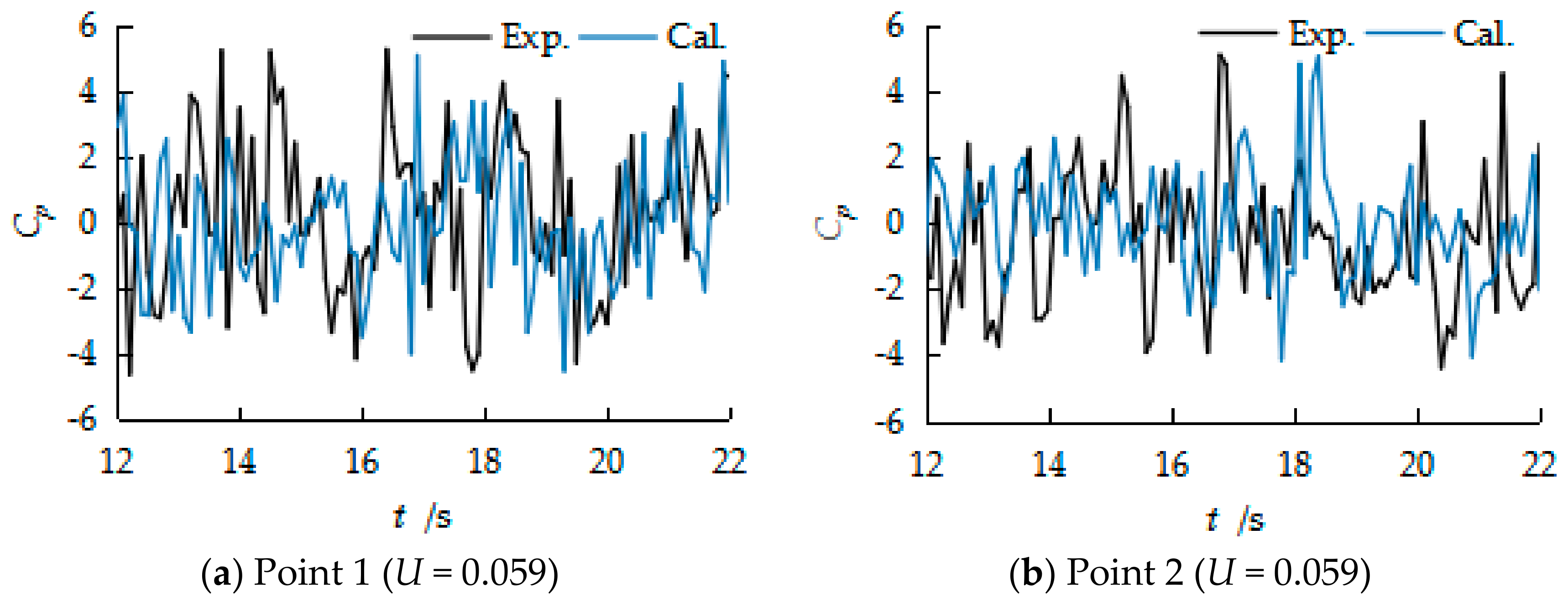
Figure 9 shows the time history curves of the fluctuating pressure coefficient of points 1 and 2 in 10 s. Cp = (p − )/0.5ρv2, where Cp is the fluctuating pressure coefficient, p is the instantaneous pressure, is the average pressure, ρ is the water flow density, and v is the average velocity of the exit section. Under the same case, the fluctuating pressure of point 1 is stronger than that of point 2. The time to reach the extreme of the two points is out of synchronization.
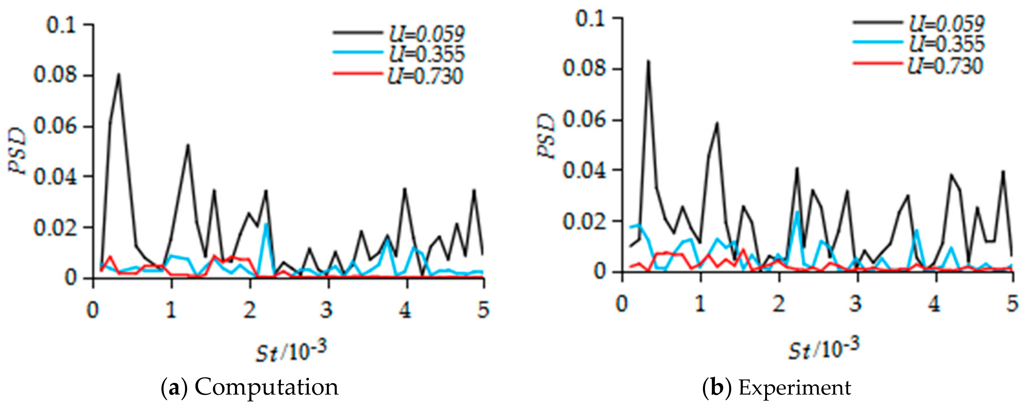
Figure 10 shows the normalized power spectrum density curve of the pressure for point 1 in different cases. St is the Strouhal number and St = f · L/, Where f is the frequency of the pressure pulsating, L is the characteristic length and taken as the gate opening, and is the mean velocity of section just below the gate. With the e/H or U increasing, the energy of pulsating pressure of point 1 decreases. The computational Strouhal numbers for dominant frequencies of the pressure are 0.332 × 10⁻³, 2.217 × 10⁻³, 1.545 × 10⁻³ with the corresponding cases of U = 0.059, 0.355, 0.730. Accordingly, the experimental Strouhal numbers for dominant frequencies of the pressure are 0.337 × 10⁻³, 2.242 × 10⁻³, 1.552 × 10⁻³ in corresponding cases. The Strouhal number difference for main frequency of the pressure between the computational and the experimental results is very small.
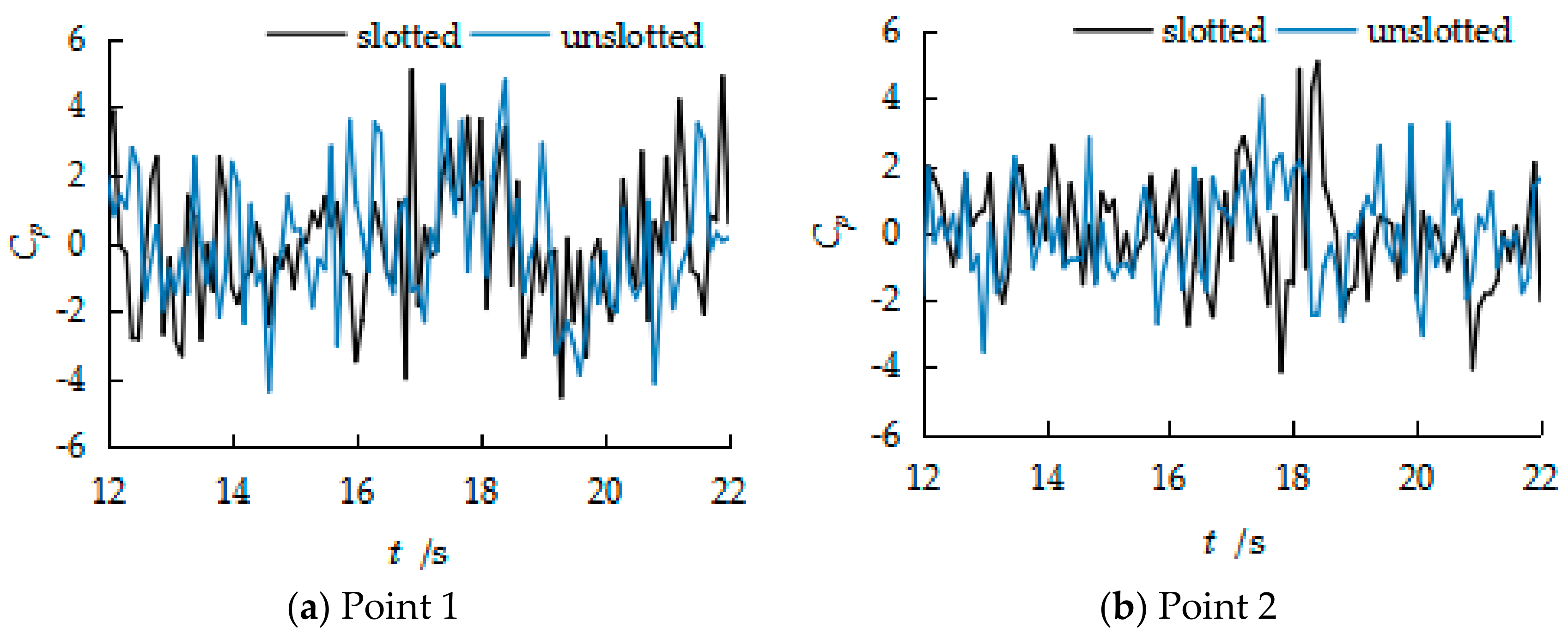
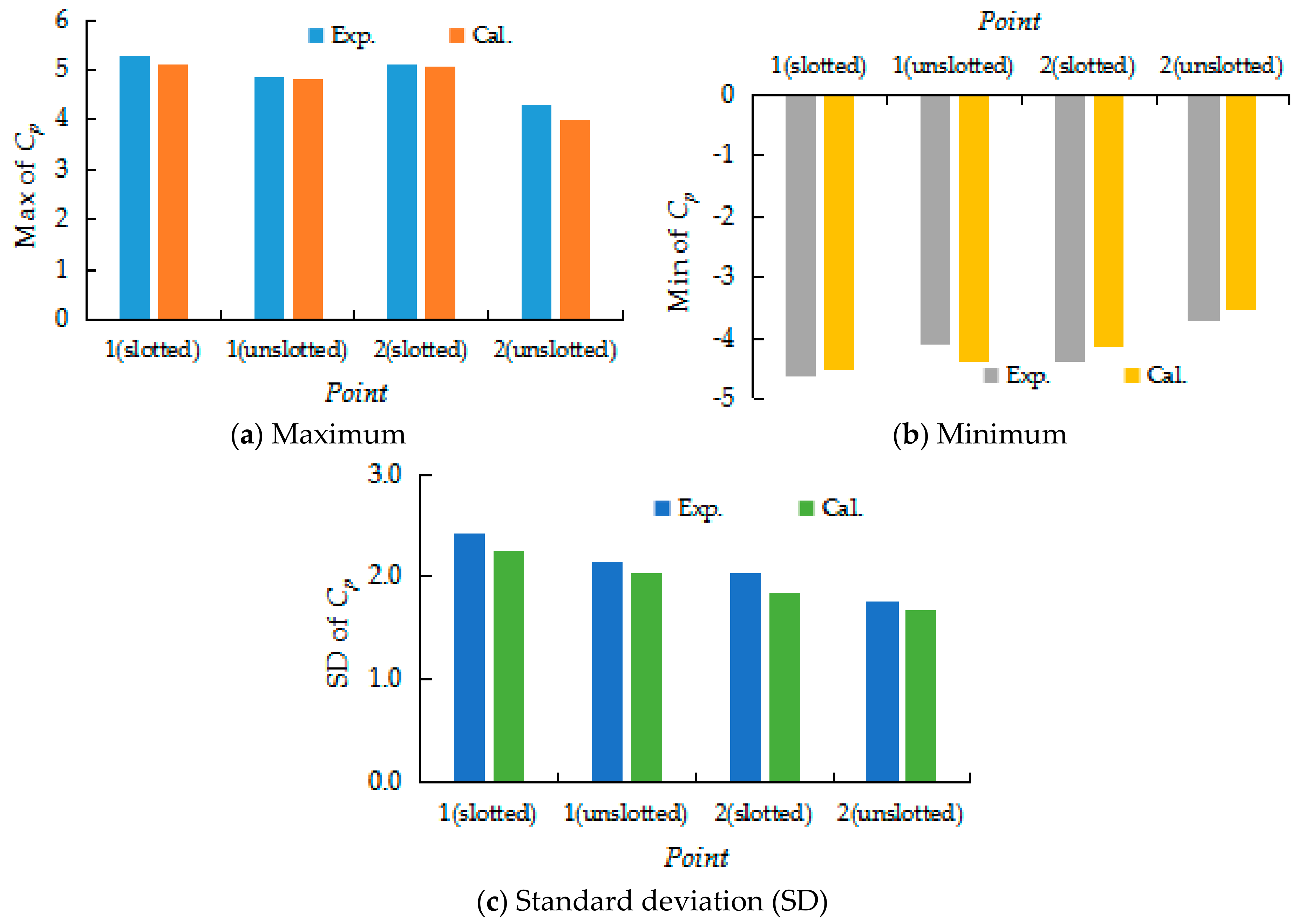
In order to illustrate the influence of the gate slot on the flow field and the gate vibration, both calculation and experiment are carried out on the filling of the slots underneath the gate (unslotted). Figure 11 shows the time history curve of the slotted and unslotted pressure pulsating coefficients in U = 0.059. It can be found that the maximum values of the slotted pressure pulsation coefficients for both points 1 and 2 were larger than those of the without a slot. The characteristic values of the pressure pulsating coefficients (slotted and unslotted) for both the experiment and for the calculation in U = 0.059 are presented in Figure 12. When comparing the value of the computational and the synchronous experimental results, the relative difference is within 10%, which indicates that the numerical simulation results meet the basic requirements.
In the experiment, the dominant frequency of the pressure at the measuring points underneath the gate are only 0.025~1.245 Hz, and the dominant frequency of the pressure at the measuring points behind the gate are only 0.183~14.63 Hz. The natural frequencies of the gate vibration by the modal analysis are 247.43 Hz, 529.85 Hz, 1086.6 Hz, 1280.6 Hz, 1605.1 Hz, and 1963.1 Hz, respectively. The natural frequency of the gate vibration is far from the dominant frequency of the flow pressure, so it would not have produced resonance.
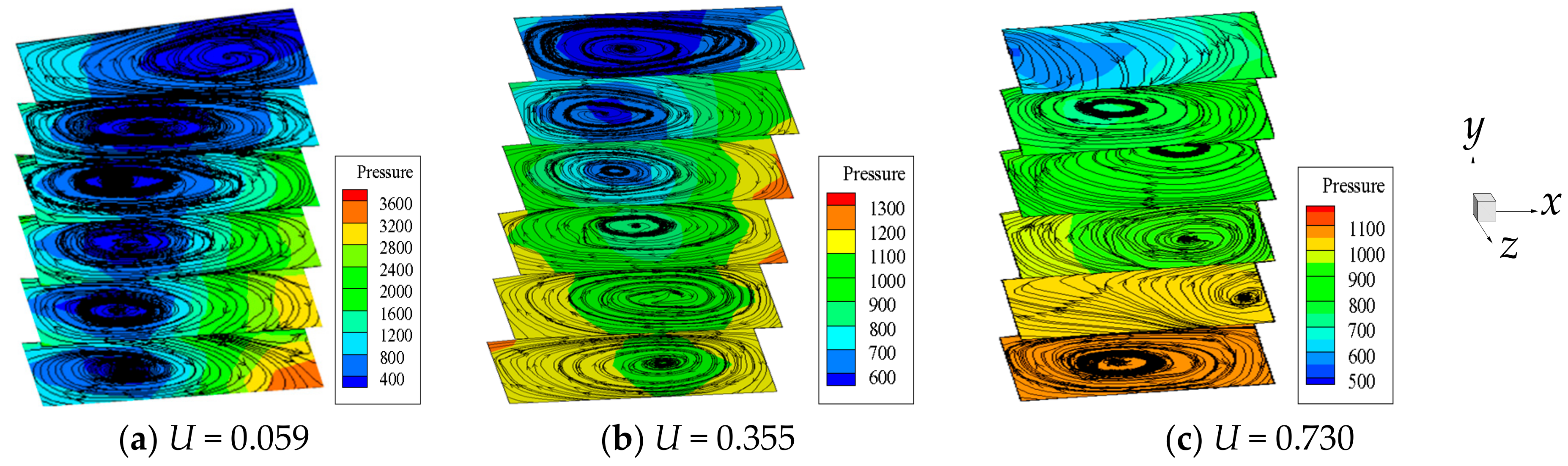
Figure 13a presents the computational pressure distribution and streamlines in the gate slot for different level cross sections (y/e = 0.067, y/e = 0.2, y/e = 0.333, y/e = 0.467, y/e = 0.6, y/e = 0.733) from the bottom to the top in y direction for U = 0.059. It can be seen from the superimposed vortex diagram that the low-pressure zone of the vortex gradually enlarges from the bottom to the top, which is shaped like a funnel and it shifted to the downstream. The pressure is lowest in the vortex center where it is also most prone to generate cavitation in the gate slot. Due to the water impacting the slot from the left to the right, the pressure is highest at the right of the slot. The closer to the bottom the place is, the higher the pressure is. Under U = 0.355 (Figure 13b) and U = 0.730 (Figure 13c), the range of the low pressure and the high pressure zones in the gate slot is much smaller than that in U = 0.059. The funnel vortex of U = 0.355 still exists, but the center of the vortex is shifted to the upstream from the bottom to the top, and the center pressure of the bottom vortex is relatively large. For U = 0.730, the centerline of the vortex is similar to the spiral line, and the funnel vortex is not obvious.
The maximum vibration displacement of the gate with a submerged condition in the x direction is not due to the resonance, but it is due to the mixed vortex-induced process, including the vortices behind the gate, in the gate slot and at the gate’s bottom edge. It can be seen from the above analysis that the numerical simulation method in this paper can obtain not only the pressure fluctuation distribution, but also a more complete flow structure, such as multiple vortices of the sluice flow, and it forms the excitation force of the plane gate vibration.
3.3. Vibration of the Gate
Define the non-dimensional coefficient Kd = (d − )/σd, where d is vibration displacement, is the average vibration displacement, and σd is the vibration standard deviation. Point A, which is located on the central axis of the upstream surface of the gate and 10 mm away from the bottom edge, is used to study the response of the gate vibration.
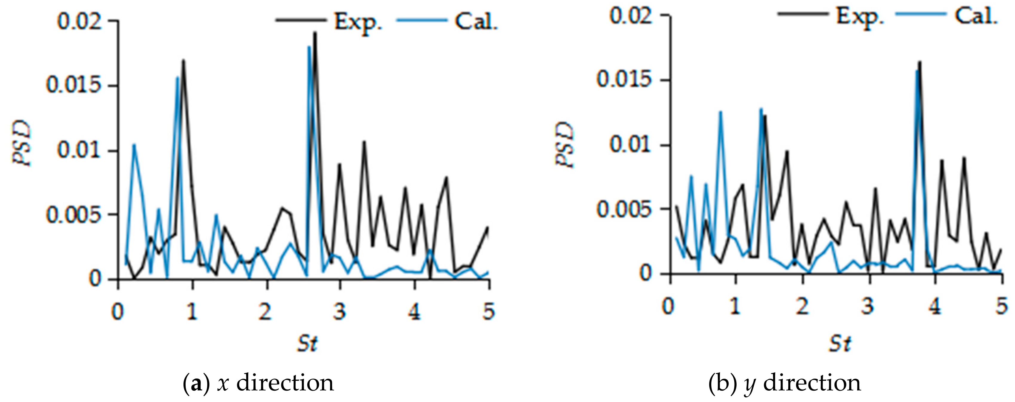
The normalized power spectrum density curve of vibration displacement for point A in U = 0.059, which is obtained by the computation and the experiment, is shown in Figure 14. In the experiment, the acceleration sensor and the multichannel data acquisition instrument were used to monitor the acceleration of the gate vibration in the x direction and y direction. The vibration displacement is achieved by the second integral of the acceleration. The computational Strouhal number for dominant frequency of vibration displacement in x direction is 2.582 with the corresponding experiment of 2.660. In addition, the computational Strouhal number for dominant frequency of vibration displacement in y direction is 3.724 with the corresponding experiment of 3.768. The Strouhal number for main frequency of the vibration displacement between the computational and the experimental results is closer.
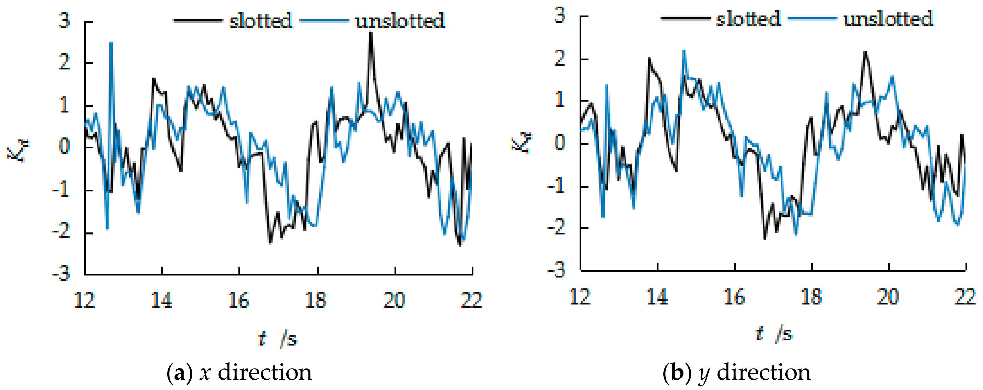
Figure 15 plots the time-history curve of the vibration displacement coefficient Kd in the x direction and in the y direction of point A, with and without slots, by using the numerical simulation. It can be seen that the maximum value of the vibration displacement coefficient of the plane gate with a slot is larger than that of the plane gate without a slot in both the x and y directions. When there is no slot, the maximum value of the x direction vibration displacement coefficient appears at 12.7 s and the minimum value appears at 21.8 s. The maximum value in the y direction appears at 14.7 s and the minimum value appears at 17.6 s. The moment when the vibration displacement coefficient of the x direction and the y direction appears is out of sync.
4. Conclusions
In this study, numerical simulations were performed to compute the flow field and the water surface profile for a plane gate with a submerged discharge by the combination of the LES and the VOF methods. Overall, the numbers and locations of the vortex are consistent with the synchronous experimental results. When compared with the experimental values, the relative difference of both the standard deviation pressure and the maximum pressure of the calculation is within 10%, which verifies the validity of the numerical simulation methods that were adopted in the present work. Simultaneously, the maximum vibration displacement coefficient was acquired from a calculation of the vibration displacement process of Point A, which was very close to that of the experiment. So, the fluid-structure coupling computational method used in certain conditions can replace the complex experiment and make up for the lack of experiment.
The turbulent kinetic energy under the gate on section z = 0 mm was higher than the value on section z = 35 mm. The change trend of the turbulent kinetic energy was consistent with the amplitude of the gate vibration displacement, which shows that the turbulent kinetic energy under the gate plays an important role in the amplitude of the gate vibration. The maximum value of the vibration displacement coefficient of the plane gate with a slot was larger than that of the plane gate without a slot in both x and y directions. Thus, the vortex in the gate slot aggravates the vibration of the gate. Turbulence pressure pulsation and multiple vortices in the flow field are the main causes of gate vibration. The mixed vortex-induced process includes the vortices behind the gate, in the gate slot, and at the gate’s bottom edge.
Author Contributions
C.S. and W.W. conceived and designed the model; C.S. and S.H. set up and debugged the programmes; C.S. analysed the results and wrote the paper; C.S. and Y.X. provided editorial improvements to the paper.
Acknowledgments
Financial support provided by the National Key Research and Development Program (Grant No. 2016YFC0401603) and the National Natural Science Foundation of China (Grant No. 51369013) are gratefully acknowledged.
Conflicts of Interest
The authors declare no conflict of interest.
References
- Hardwick, J.D. Flow-induced vibration of vertical lift gate. J. Hydraul. Div. 1974, 100, 631–644. [Google Scholar]
- Kolkman, P.A.; Vrijer, A. Gate edge suction as a cause of self-exciting vertical vibrations. In Proceedings of the 17th IAHR Congress, Baden, Germany, 15–19 August 1977; Volume 17, pp. 425–437. [Google Scholar]
- Jongeling, T.H.G. Flow-induced Self-excited in Flow Vibrations of Gate Plates. J. Fluids Struct. 1988, 2, 541–566. [Google Scholar] [CrossRef]
- Ishii, N. Flow-induced vibration of long span gates, Part I: Model development. J. Fluids Struct. 1992, 6, 539–562. [Google Scholar] [CrossRef]
- Pani, P.K.; Bhattacharyya, S.K. Hydrodynamic pressure on a vertical gate considering fluid-structure interaction. Finite Elem. Anal. Des. 2008, 44, 759–766. [Google Scholar] [CrossRef]
- Erdbrink, C.D.; Krzhizhanovskaya, V.V.; Sloot, P.M.A. Reducing cross-flow vibrations of underflow gates: Experiments and numerical studies. J. Fluids Struct. 2014, 50, 25–48. [Google Scholar] [CrossRef]
- Liu, S.; Liao, T.; Luo, Q. Numerical simulation of turbulent flow behind sluice gate under submerged discharge conditions. J. Hydrodyn. 2015, 27, 257–263. [Google Scholar] [CrossRef]
- Kotecki, S.W. Numerical modeling of flow through moving water-control gates by vortex method. Part I—Problem formulation. Arch. Civ. Mech. Eng. 2008, 8, 73–89. [Google Scholar] [CrossRef]
- Kotecki, S.W. Numerical modeling of flow through moving water-control gates by vortex method. Part II—Calculation result. Arch. Civ. Mech. Eng. 2008, 8, 39–49. [Google Scholar] [CrossRef]
- Kotecki, S.W. Numerical analysis of hydrodynamic forces due to flow instability at lift gate. Arch. Civ. Mech. Eng. 2011, 11, 943–961. [Google Scholar] [CrossRef]
- Kazemzadeh-Parsi, M.J. Numerical flow simulation in gated hydraulic structures using smoothed fixed grid finite element method. Appl. Math. Comput. 2014, 246, 447–459. [Google Scholar] [CrossRef]
- Zhu, T.; Ye, W. Theoretical and numerical studies of noncontinuum gas-phase heat conduction in micro/nano devices. Numer. Heat Transf. Part B Fundam. 2010, 57, 203–226. [Google Scholar] [CrossRef]
- Liu, H.; Xu, K.; Zhu, T.; Ye, W. Multiple temperature kinetic model and its applications to micro-scale gas flows. Comput. Fluids 2012, 67, 115–122. [Google Scholar] [CrossRef] [Green Version]
- He, S.; Zhang, L. Large Eddy Simulation of Effect of Geometric Parameters on Low Pressure of Turbulent Flow over Gate Slot. J. Syst. Simul. 2015, 27, 1081–1086. [Google Scholar]
- Leclercq, T.; de Langre, E. Vortex-induced vibrations of cylinders bent by the flow. J. Fluids Struct. 2018, 80, 77–93. [Google Scholar] [CrossRef]
- Chizfahm, A.; Yazdi, E.A.; Eghtesad, M. Dynamic modeling of vortex induced vibration wind turbines. Renew. Energy 2018, 121, 632–643. [Google Scholar] [CrossRef]
- Postnikov, A.; Pavlovskaia, E.; Wiercigroch, M. 2DOF CFD calibrated wake oscillator model to investigate vortex-induced vibrations. Int. J. Mech. Sci. 2017, 127, 176–190. [Google Scholar] [CrossRef] [Green Version]
- Bouratsis, P.; Diplas, P.; Dancey, C.L.; Apsilidis, N. Quantitative Spatio-Temporal Characterization of Scour at the Base of a Cylinder. Water 2017, 9, 227. [Google Scholar] [CrossRef]
- Smagorinsky, J. General circulation experiment with primitive equations. Mon. Weather Rev. 1963, 91, 99–164. [Google Scholar] [CrossRef]
- Lilly, D.K. Aproposed modification of the Germa no subgrid-scale closure method. Phys. Fluid A 1992, 4, 633–635. [Google Scholar] [CrossRef]
- Shen, C.; He, S.; Yang, T.; Wang, W. Model tests for synchronous measurement of fluid-structure interaction vibration of a plane vertical lift gate. J. Vib. Shock 2016, 35, 219–224. [Google Scholar]
Figure 1.
The grid of fluid.

Figure 2.
The plane gate: (a) the grid; and, (b) the size (unit: mm).

Figure 3.
General arrangement of the experiment.

Figure 4.
The color nephogram of the time-averaged flow profile.

Figure 5.
The time-averaged flow profile.

Figure 6.
The calculational time-averaged streamlines.

Figure 7.
The instantaneous streamlines (z = 0 mm).


Figure 8.
Normalized turbulent kinetic energy distribution.


Figure 9.
The time history curve of the pressure pulsating coefficient for different point.

Figure 10.
The power spectrum density (PSD) curve of the pressure for point 1 in different cases.

Figure 11.
The time history curve of the pressure pulsating coefficients (slotted and unslotted).

Figure 12.
The comparison of characteristic value of the pressure pulsating coefficient.

Figure 13.
Pressure (pa) distribution and streamlines at 22.0 s in the gate slot.

Figure 14.
The power spectrum density (PSD) curve of vibration displacement for point A.

Figure 15.
The time history curve of the vibration displacement coefficient Kd of point A.


Table 1.
A list of the cases of calculation.
| Case | e/H | U |
|---|---|---|
| 1 | 0.049 | 0.059 |
| 2 | 0.197 | 0.355 |
| 3 | 0.375 | 0.730 |
© 2018 by the authors. Licensee MDPI, Basel, Switzerland. This article is an open access article distributed under the terms and conditions of the Creative Commons Attribution (CC BY) license (http://creativecommons.org/licenses/by/4.0/).
Share and Cite
MDPI and ACS Style
Shen, C.; Wang, W.; He, S.; Xu, Y. Numerical and Experimental Comparative Study on the Flow-Induced Vibration of a Plane Gate. Water 2018, 10, 1551. https://doi.org/10.3390/w10111551
AMA Style
Shen C, Wang W, He S, Xu Y. Numerical and Experimental Comparative Study on the Flow-Induced Vibration of a Plane Gate. Water. 2018; 10(11):1551. https://doi.org/10.3390/w10111551
Chicago/Turabian StyleShen, Chunying, Wei Wang, Shihua He, and Yimin Xu. 2018. "Numerical and Experimental Comparative Study on the Flow-Induced Vibration of a Plane Gate" Water 10, no. 11: 1551. https://doi.org/10.3390/w10111551
Note that from the first issue of 2016, this journal uses article numbers instead of page numbers. See further details here.