Drought Propagation in Semi-Arid River Basins in Latin America: Lessons from Mexico to the Southern Cone

 ,
,  , and
, and
Abstract
:1. Introduction
2. Data and Methods
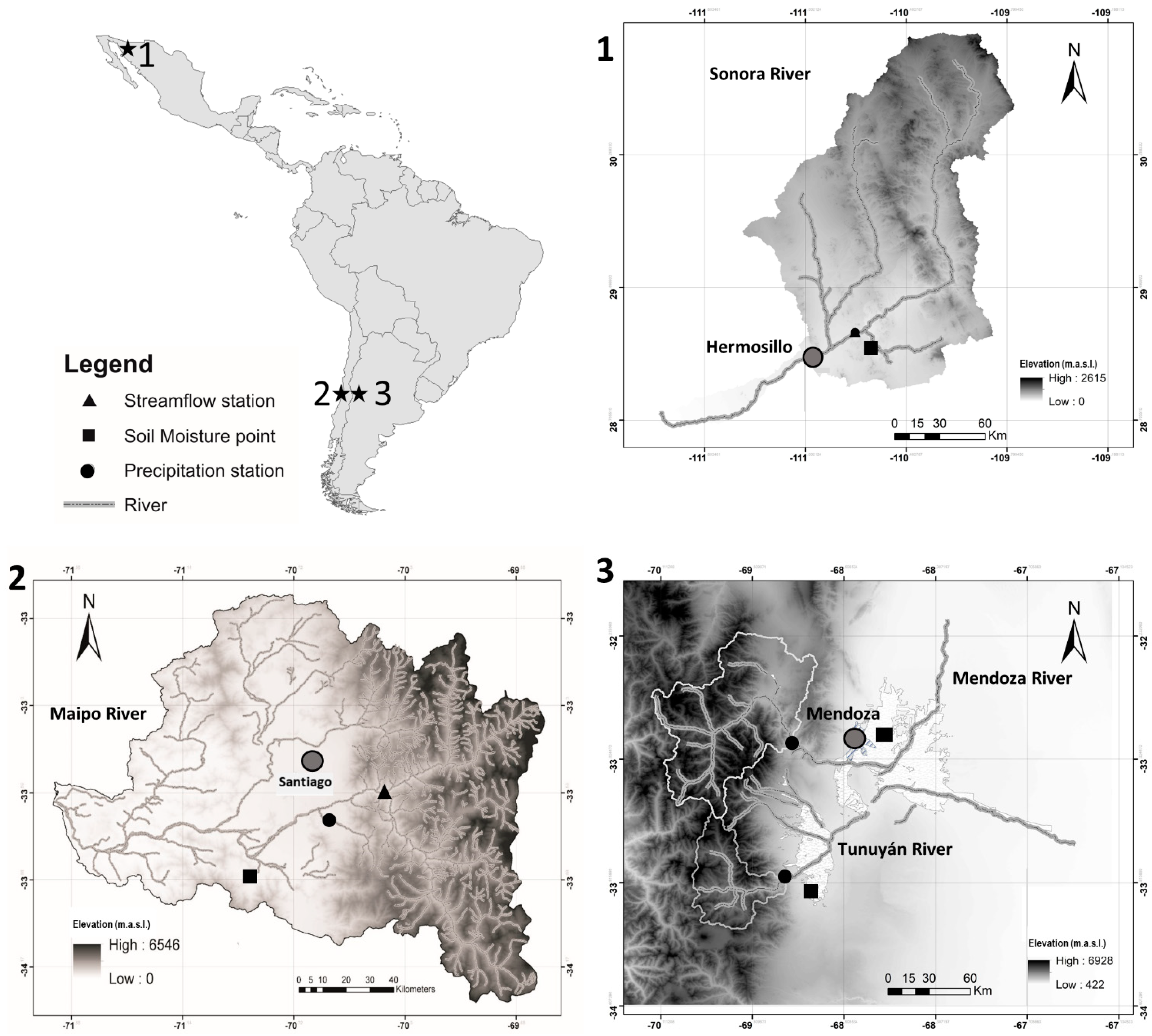
2.1. River Basins
2.1.1. Sonora, Mexico
2.1.2. Maipo, Chile
2.1.3. Mendoza-Tunuyán, Argentina
2.2. Data
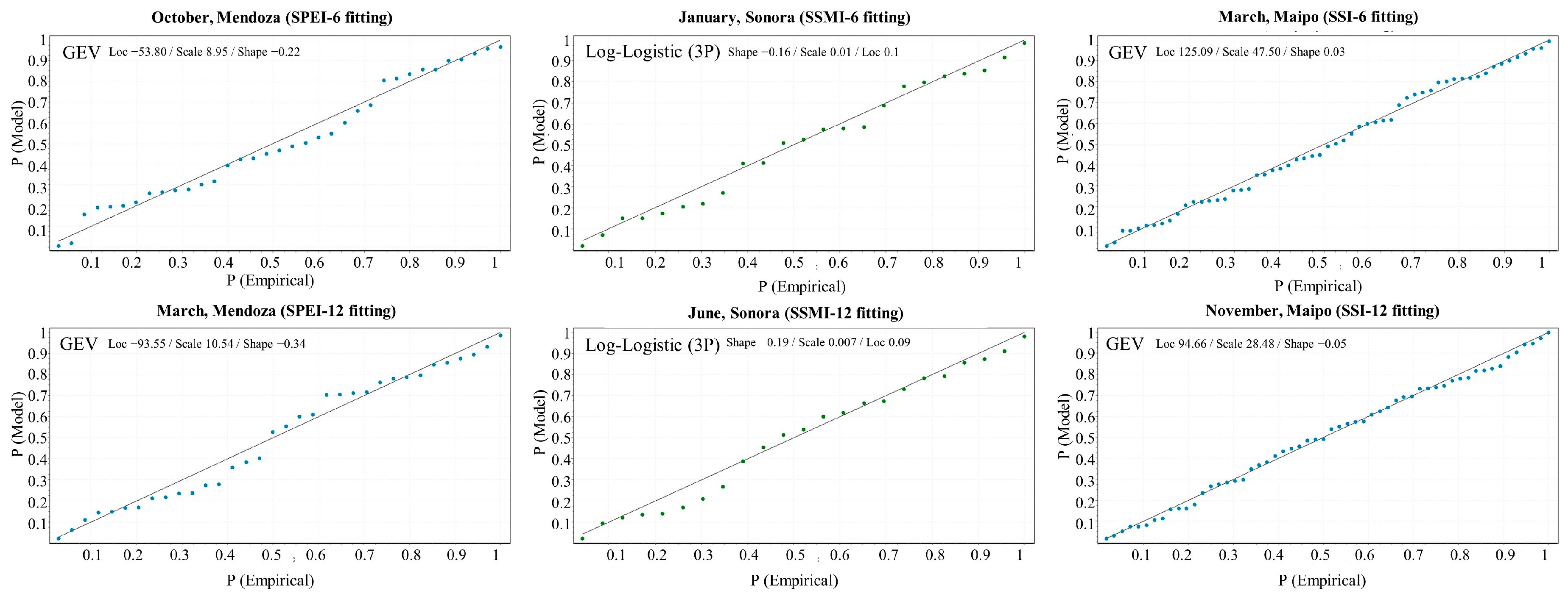
2.3. Standardized Indices
- obtaining the time series of the desired variable at a given time step (e.g., monthly),
- fitting a probability distribution function to monthly data aggregated using different cumulative periods (e.g., 1-, 3-, 6-, 12-month),
- converting to a cumulative distribution function, and
- use an inverse function to obtain standardized gaussian values (i.e., values that follow a normal distribution with mean 0 and standard deviation 1).
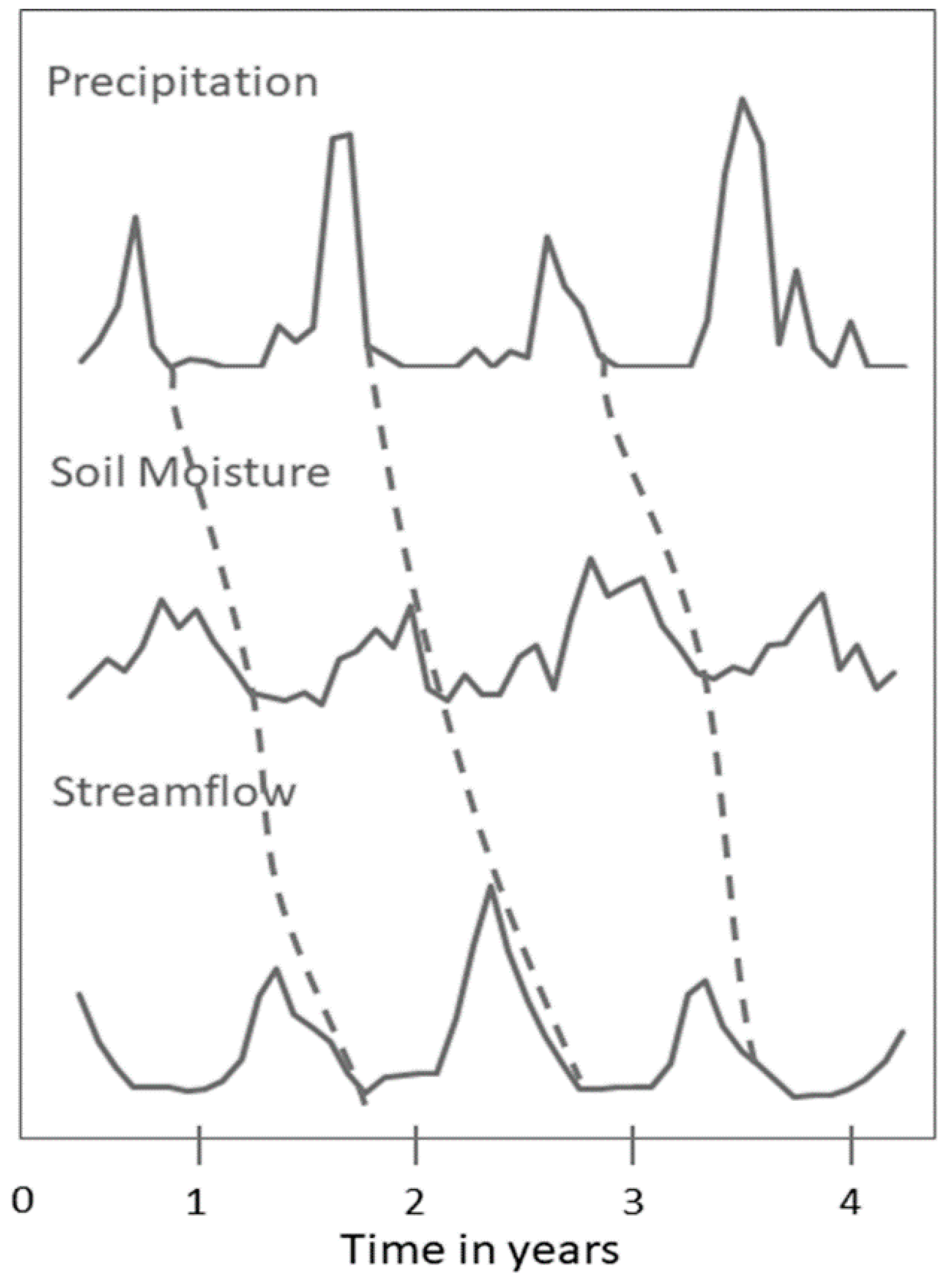
2.4. Drought Propagation
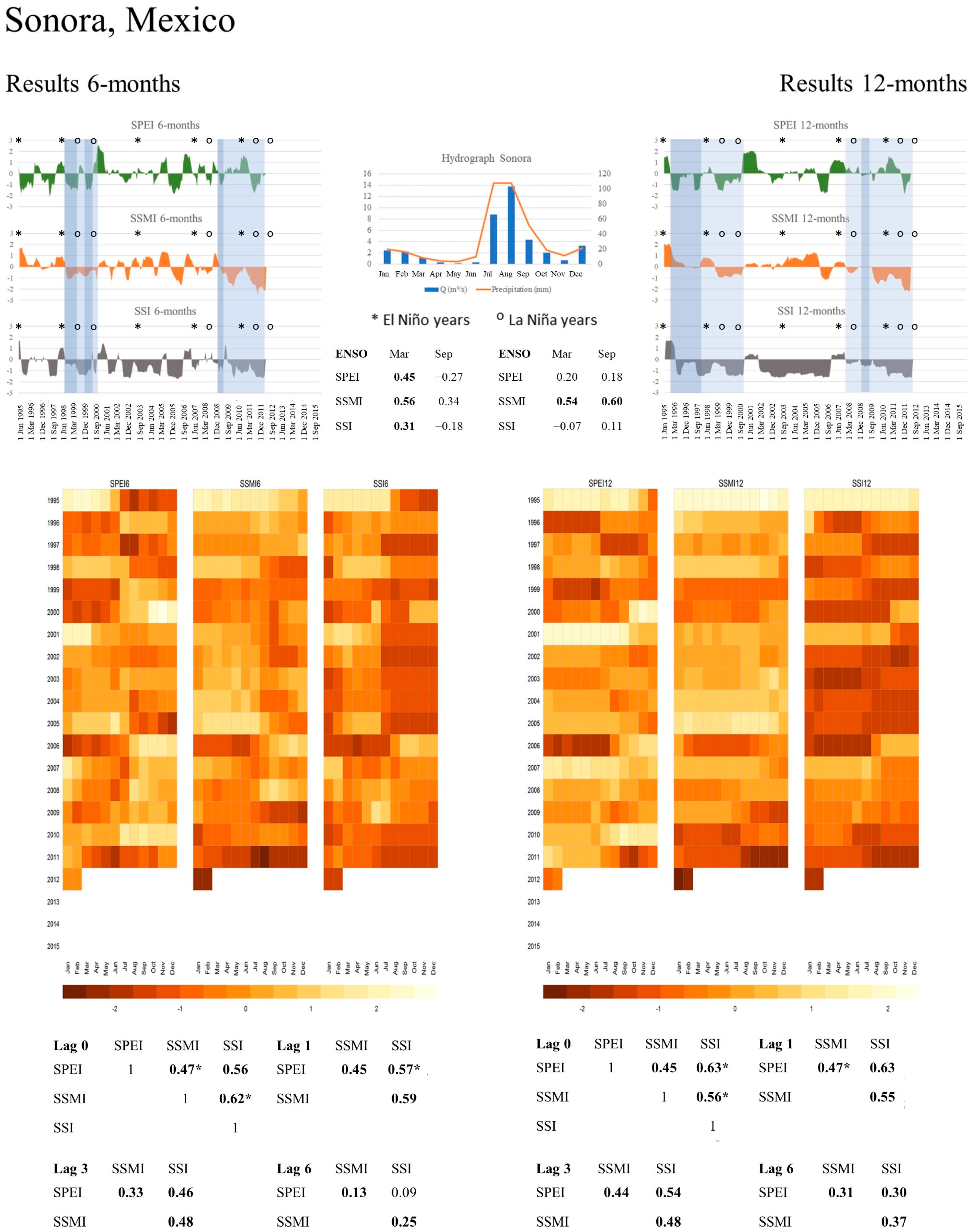
2.5. ENSO Influence
3. Results
3.1. Sonora, Mexico
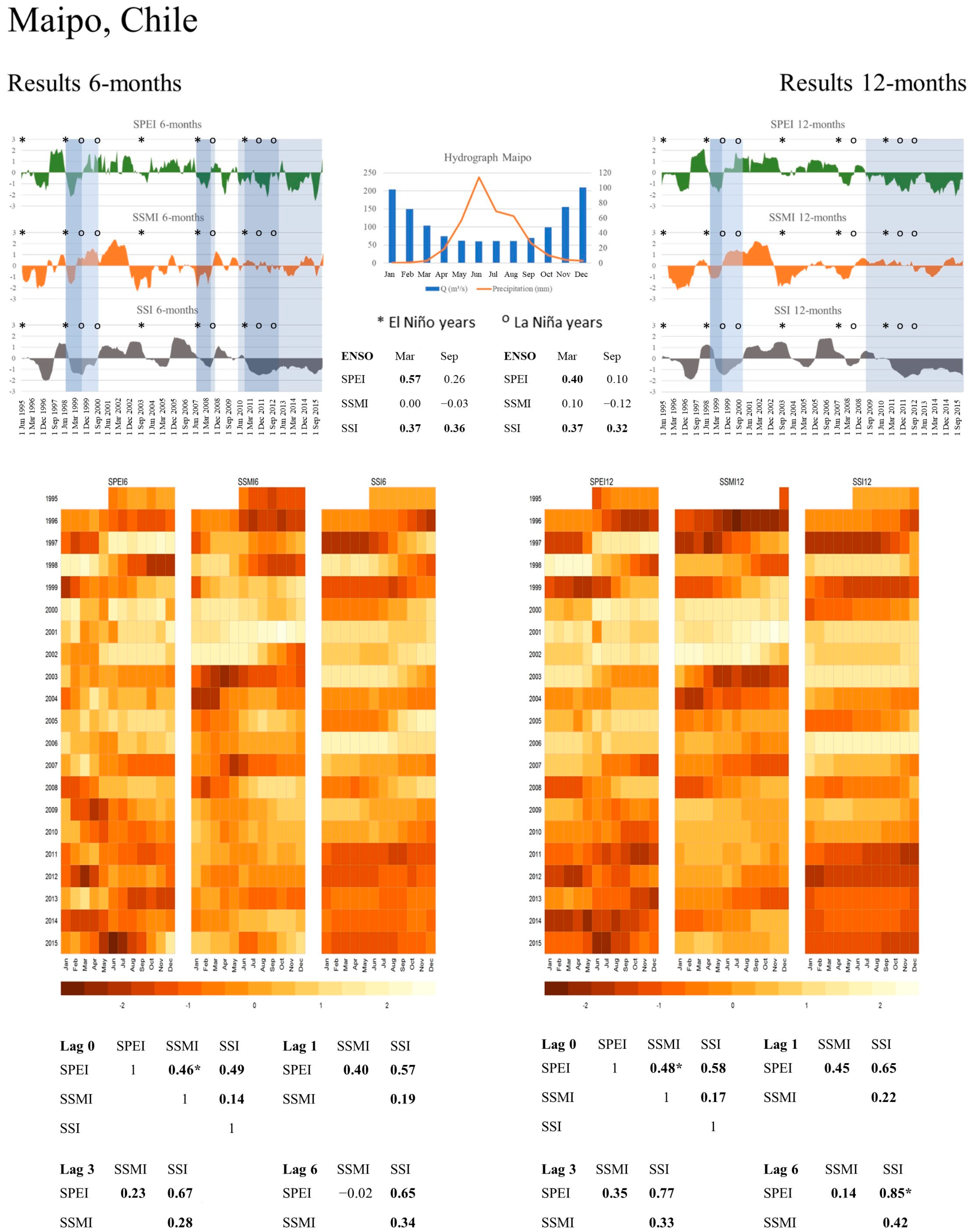
3.2. Maipo, Chile
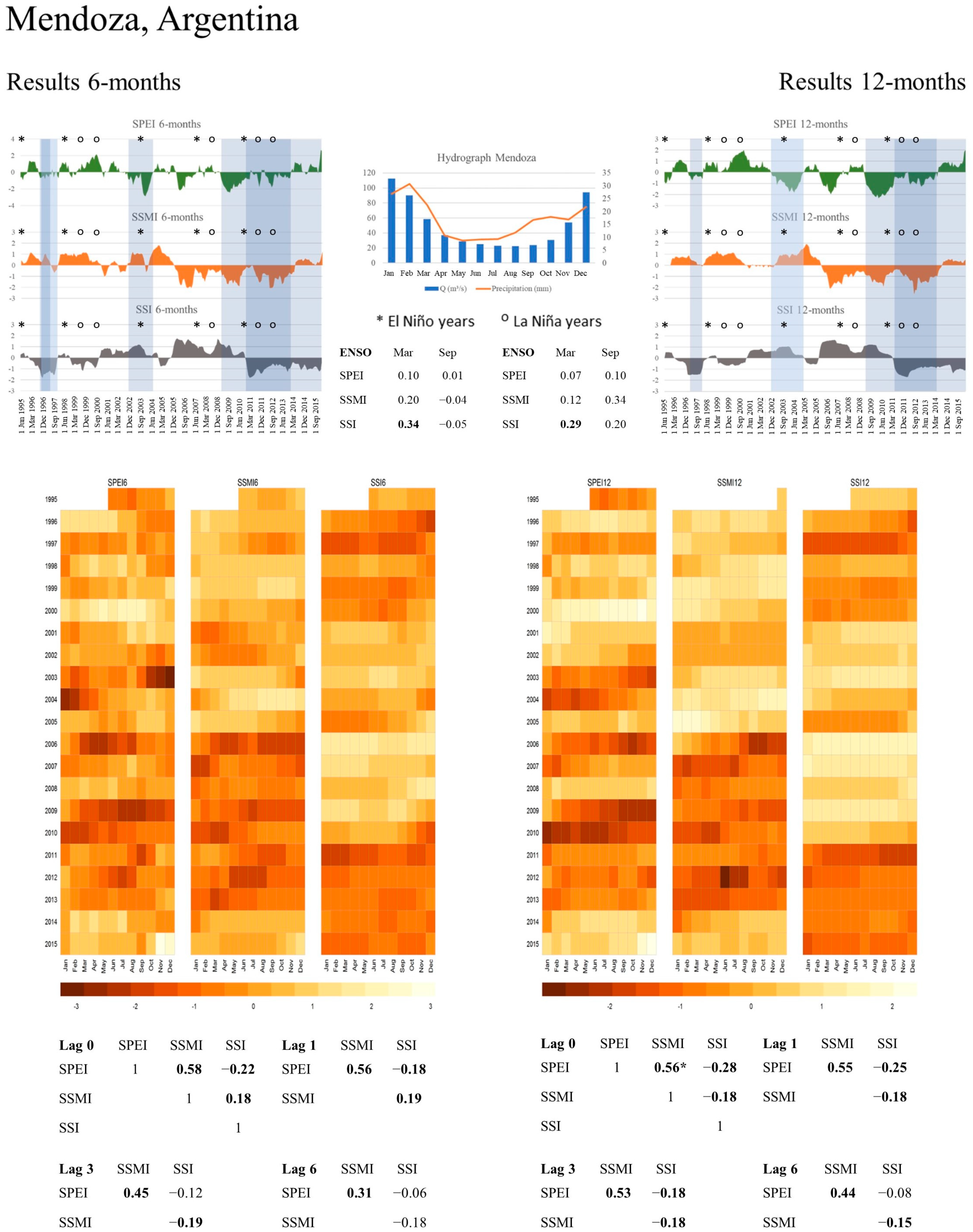
3.3. Mendoza, Argentina
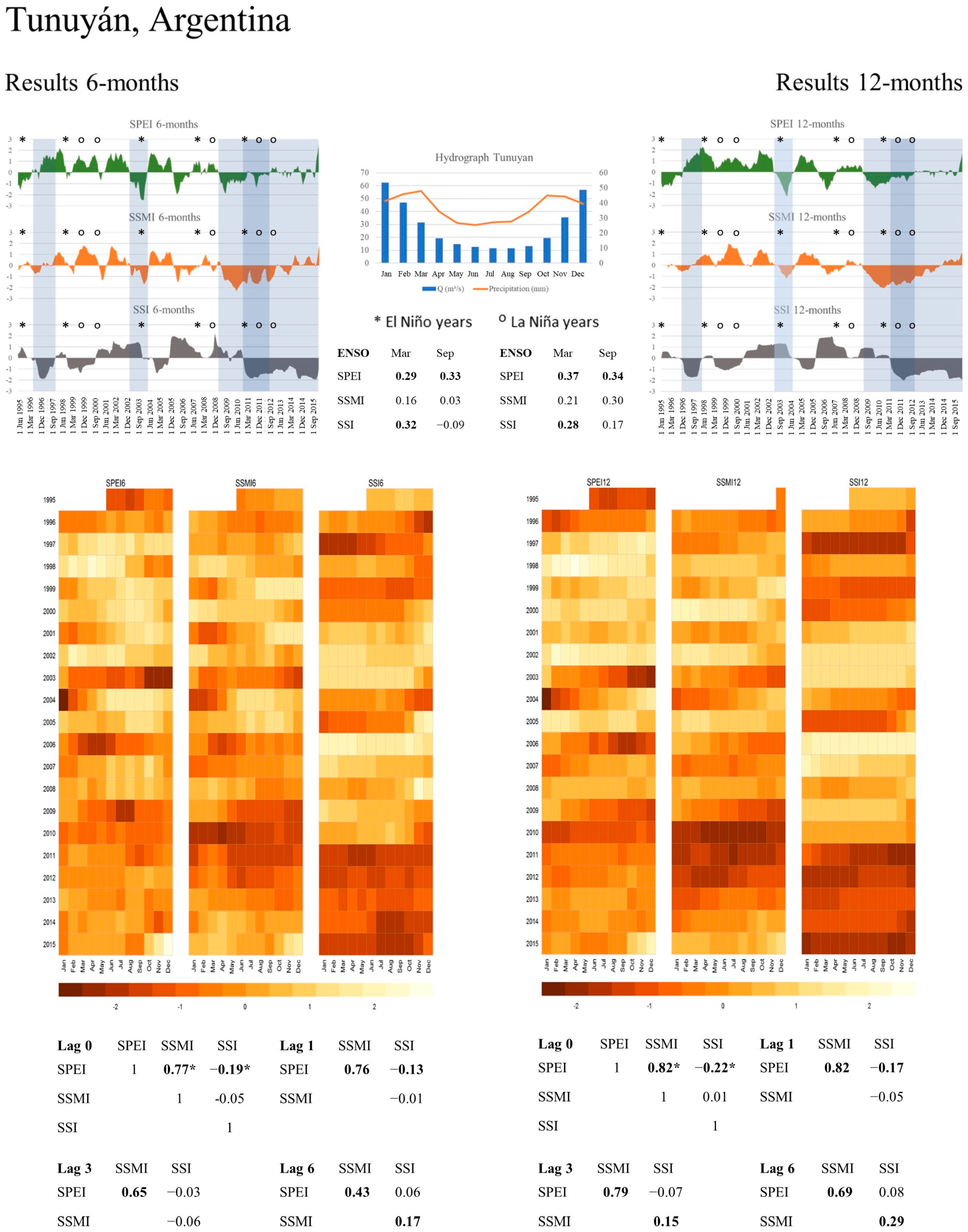
3.4. Tunuyán, Argentina
4. Discussion
4.1. “Interconnected” Andes
4.2. Drought Propagation via Standardized Indices
5. Conclusions
Author Contributions
Funding
Acknowledgments
Conflicts of Interest
References
- Ding, Y.; Hayes, M.J.; Widhalm, M. Measuring economic impacts of drought: A review and discussion. Disaster Prev. Manag. 2011, 20, 434–446. [Google Scholar] [CrossRef]
- Wilhite, D.A.; Glantz, M.H. Understanding the drought phenomenon: The role of definitions. Water Int. 1985, 10, 111–120. [Google Scholar] [CrossRef]
- AghaKouchak, A. Recognize anthropogenic drought. Nature 2015, 524, 409–411. [Google Scholar] [CrossRef] [PubMed]
- Van Dijk, A.I.J.M.; Beck, H.E.; Crosbie, R.S.; de Jeu, R.A.M.; Liu, Y.Y.; Podger, G.M.; Timbal, B.; Viney, N.R. The Millennium Drought in southeast Australia (2001–2009): Natural and human causes and implications for water resources, ecosystems, economy, and society. Water Resour. Res. 2013, 49, 1040–1057. [Google Scholar] [CrossRef]
- Peters, E.; Bier, G.; van Lanen, H.A.J.; Torfs, P.J.J.F. Propagation and spatial distribution of drought in a groundwater catchment. J. Hydrol. 2006, 321, 257–275. [Google Scholar] [CrossRef]
- Wood, E.F.; Sheffield, J. Drought: Past Problems and Future Scenarios; Taylor and Francis: Hoboken, NJ, USA, 2012. [Google Scholar]
- Changnon, S.A. Detecting Drought Conditions in Illinois; Department of Energy and Natural Resources: Springfield, IL, USA, 1987. [Google Scholar]
- Van Lanen, H.A.J. Drought propagation through the hydrological cycle. In Climate Variability and Change, Proceedings of the Fifth Friend World Conference, Havana, Cuba, 27 November–1 December 2006; IAHS Press: Wallingford, UK, 2006. [Google Scholar]
- Tallaksen, L.M.; Hisdal, H.; van Lanen, H.A.J. Space–time modelling of catchment scale drought characteristics. J. Hydrol. 2009, 375, 363–372. [Google Scholar] [CrossRef]
- Van Loon, A.F. On the Propagation of Drought. Ph.D. Thesis, Wageningen University, Wageningen, The Netherlands, 2013. [Google Scholar]
- Barker, L.J.; Hannaford, J.; Chiverton, A.; Svensson, C. From meteorological to hydrological drought using standardised indicators. Hydrol. Earth Syst. Sci. 2016, 20, 2483–2505. [Google Scholar] [CrossRef]
- Liu, Y.Y.; Dorigo, W.A.; Parinussa, R.M.; de Jeu, R.A.M.; Wagner, W.; McCabe, M.F.; Evans, J.P.; van Dijk, A.I.J.M. Trend-preserving blending of passive and active microwave soil moisture retrievals. Remote Sens. Environ. 2012, 123, 280–297. [Google Scholar] [CrossRef]
- Dorigo, W.; Wagner, W.; Albergel, C.; Albrecht, F.; Balsamo, G.; Brocca, L.; Chung, D.; Ertl, M.; Forkel, M.; Gruber, A.; et al. ESA CCI Soil Moisture for improved Earth system understanding: State-of-the art and future directions. Remote Sens. Environ. 2017, 203, 185–215. [Google Scholar] [CrossRef]
- Gruber, A.; Dorigo, W.A.; Crow, W.; Wagner, W. Triple Collocation-Based Merging of Satellite Soil Moisture Retrievals. IEEE Trans. Geosci. Remote Sens. 2017, 55, 6780–6792. [Google Scholar] [CrossRef]
- Keshavarz, M.R.; Vazifedoust, M.; Alizadeh, A. Drought monitoring using a Soil Wetness Deficit Index (SWDI) derived from MODIS satellite data. Agric. Water Manag. 2014, 132, 37–45. [Google Scholar] [CrossRef]
- Mishra, A.; Vu, T.; Veettil, A.V.; Entekhabi, D. Drought monitoring with soil moisture active passive (SMAP) measurements. J. Hydrol. 2017, 552, 620–632. [Google Scholar] [CrossRef]
- Martínez-Fernández, J.; González-Zamora, A.; Sánchez, N.; Gumuzzio, A.; Herrero-Jiménez, C.M. Satellite soil moisture for agricultural drought monitoring: Assessment of the SMOS derived Soil Water Deficit Index. Remote Sens. Environ. 2016, 177, 277–286. [Google Scholar] [CrossRef]
- Kędzior, M.; Zawadzki, J. SMOS data as a source of the agricultural drought information: Case study of the Vistula catchment, Poland. Geoderma 2017, 306, 167–182. [Google Scholar] [CrossRef]
- Instituto Nacional de Estadística y Geografía (INEGI). Censo de Población y Vivienda 2010. 2016. Available online: http://www.beta.inegi.org.mx/proyectos/ccpv/2010/ (accessed on 19 January 2018).
- Robles-Morua, A.; Halvorsen, K.E.; Mayer, A.S.; Vivoni, E.R. Exploring the application of participatory modeling approaches in the Sonora River Basin, Mexico. Environ. Model. Softw. 2014, 52, 273–282. [Google Scholar] [CrossRef]
- Romo-Leon, J.R.; van Leeuwen, W.J.D.; Castellanos-Villegas, A. Using remote sensing tools to assess land use transitions in unsustainable arid agro-ecosystems. J. Arid Environ. 2014, 106, 27–35. [Google Scholar] [CrossRef]
- Pineda-Pablos, N.; Moreno-Váquez, J.-L.; Salazar-Adams, A.; Lutz-Ley, A.N. Derechos de agua y gestión por cuencas en México. El caso del río Sonora. Espiral Estud. Sobre Estado Soc. 2014, 21, 191–225. [Google Scholar]
- Comisión Nacional del Agua (CONAGUA). Programas de Medidas Preventivas y de Mitigación de la Sequía: Guía de Elaboración para Usuarios Urbanos de agua Potable y Sanemiento; Versión 1.0; Comisión Nacional del Agua: Mexico City, Mexico, 2014. [Google Scholar]
- Adams, A.; Vázquez, J.L.; Ley, A.N. Agricultura y manejo sustentable del acuífero de la Costa de Hermosillo. Reg. Soc. 2012, 54, 155–179. [Google Scholar]
- Meza, F.J.; Vicuña, S.; Jelinek, M.; Bustos, E.; Bonelli, S. Assessing water demands and coverage sensitivity to climate change in the urban and rural sectors in central Chile. J. Water Clim. Chang. 2014, 5, 192. [Google Scholar] [CrossRef]
- Meza, F.; Wilks, D.; Gurovich, L.; Bambach, N. Impacts of climate change on irrigated agriculture in the Maipo Basin, Chile: Reliability of water rights and changes in the demand for irrigation. J. Water Resour. Plan. Manag. 2012, 138, 421–430. [Google Scholar] [CrossRef]
- Garreaud, R.; Alvarez-Garreton, C.; Barichivich, J.; Boisier, J.P.; Christie, D.; Galleguillos, M.; LeQuesne, C.; McPhee, J.; Zambrano-Bigiarini, M. The 2010–2015 mega drought in Central Chile: Impacts on regional hydroclimate and vegetation. Hydrol. Earth Syst. Sci. 2017, 21, 6307–6327. [Google Scholar] [CrossRef]
- Bustos, E.; Meza, F.J. A method to estimate maximum and minimum air temperature using MODIS surface temperature and vegetation data: Application to the Maipo Basin, Chile. Theor. Appl. Climatol. 2015, 120, 211–226. [Google Scholar] [CrossRef]
- Departamento General de Irrigación (DGI). Plan Director del Rio Mendoza; Gobierno de Mendoza, Secretaría de Agricultura, Ganadería, Pesca y Alimentación de la Nación, Proyecto PNUD/FAO/ARG/00/008; DGI: Mendoza, Argentina, 2006. [Google Scholar]
- Departamento General de Irrigación (DGI). Plan Director del Rio Tunuyán; Gobierno de Mendoza, Secretaría de Agricultura, Ganadería, Pesca y Alimentación de la Nación, Proyecto PNUD/FAO/ARG/00/008; DGI: Mendoza, Argentina, 2006. [Google Scholar]
- Castex, V.; Tejeda, E.M.; Beniston, M. Water availability, use and governance in the wine producing region of Mendoza, Argentina. Environ. Sci. Policy 2015, 48, 1–8. [Google Scholar] [CrossRef] [Green Version]
- Salatino, S.; Morábito, J.; Bermejillo, A.; Dediol, C.; Stocco, A.; Tapia, O.; Miralles, S.; Hernández, R.; Mastrantonio, L.; Genovese, D.; et al. Calidad de aguas y análisis de la contaminación en el Río Tunuyán Superior (Mendoza, Argentina) en el periodo 2007–2014: Water quality and analysis of contamination in upper Tunuyán River (Mendoza, Argentina) in period 2007–2014. Augmdomus 2017, 9, 67–82. [Google Scholar]
- Salas, S.; Jiménez, E.; Montaña, E.; Garay-Flühmann, R.; Gauthier, D.; Polo Díaz, H. Vulnerabilidad al Cambio Climático: Desafíos para la Adaptación en las Cuencas de Elqui y Mendoza; Inter-American Institute for Global Change Research: Montevideo, Uruguay, 2012. [Google Scholar]
- Guttmann, N. Accepting the standardized precipitation index: A calculation algorithm. J. Am. Water Resour. Assoc. 1999, 35, 311–322. [Google Scholar] [CrossRef]
- World Meteorological Organization (WMO). Standardized Precipitation Index User Guide; Svoboda, M., Hayes, M., Wood, D., Eds.; World Meteorological Organization: Geneva, Switzerland, 2012. [Google Scholar]
- Otkin, J.A.; Anderson, M.C.; Hain, C.; Svoboda, M. Using temporal changes in drought indices to generate probabilistic drought intensification forecasts. J. Hydrometeorol. 2014. [Google Scholar] [CrossRef]
- Pappas, C.; Papalexiou, S.M.; Koutsoyiannis, D. A quick gap filling of missing hydrometeorological data. J. Geophys. Res. Atmos. 2014, 119, 9290–9300. [Google Scholar] [CrossRef] [Green Version]
- McKee, T.; Doesken, N.; Kleist, J. The relationship of drought frequency and duration to time scales. In Proceedings of the Eight Conference, Anaheim, CA, USA, 17–22 January 1993; pp. 179–184. [Google Scholar]
- Heim, R.R. A review of twentieth-century drought indices used in the United States. Bull. Am. Meteorol. Soc. 2002, 1149–1165. [Google Scholar] [CrossRef]
- Mishra, A.K.; Singh, V.P. Drought modeling—A review. J. Hydrol. 2011, 403, 157–175. [Google Scholar] [CrossRef]
- Quiring, S.M. Developing objective operational definitions for monitoring drought. J. Appl. Meteorol. Climatol. 2009, 48, 1217–1229. [Google Scholar] [CrossRef]
- Guttman, N.B. Comparing the palmer drought index and the standardized precipitation index. J. Am. Water Resour. Assoc. 1998, 34, 113–121. [Google Scholar] [CrossRef]
- Sivakumar, M.V.K.; Motha, R.P.; Wilhite, D.A.; Wood, D.A. (Eds.) Agricultural Drought Indices, 1572nd ed.; World Meteorological Organization: Geneva, Switzerland, 2011. [Google Scholar]
- Vicente-Serrano, S.M.; Beguería, S.; López-Moreno, J.I. A multiscalar drought index sensitive to global warming: The standardized precipitation evapotranspiration index. J. Clim. 2010, 23, 1696–1718. [Google Scholar] [CrossRef]
- Droogers, P.; Allen, R.G. Estimating reference evapotranspiration under inaccurate data conditions. Irrig. Drain. Syst. 2002, 16, 33–45. [Google Scholar] [CrossRef]
- Beguería, S.; Vicente-Serrano, S.M.; Reig, F.; Latorre, B. Standardized precipitation evapotranspiration index (SPEI) revisited: Parameter fitting, evapotranspiration models, tools, datasets and drought monitoring. Int. J. Climatol. 2014, 34, 3001–3023. [Google Scholar] [CrossRef]
- Stagge, J.H.; Tallaksen, L.M.; Gudmundsson, L.; van Loon, A.F.; Stahl, K. Candidate distributions for climatological drought indices (SPI and SPEI). Int. J. Climatol. 2015, 35, 4027–4040. [Google Scholar] [CrossRef]
- Stagge, J.H.; Tallaksen, L.M.; Gudmundsson, L.; van Loon, A.F.; Stahl, K. Response to comment on ‘Candidate distributions for climatological drought indices (SPI and SPEI)’. Int. J. Climatol. 2016, 36, 2132–2138. [Google Scholar] [CrossRef]
- Vicente-Serrano, S.M.; Beguería, S. Comment on ‘Candidate distributions for climatological drought indices (SPI and SPEI)’ by James H. Stagge et al. Int. J. Climatol. 2016, 36, 2120–2131. [Google Scholar] [CrossRef]
- Carrão, H.; Russo, S.; Sepulcre-Canto, G.; Barbosa, P. An empirical standardized soil moisture index for agricultural drought assessment from remotely sensed data. Int. J. Appl. Earth Obs. Geoinf. 2016, 48, 74–84. [Google Scholar] [CrossRef]
- Hao, Z.; AghaKouchak, A. Multivariate standardized drought index: A parametric multi-index model. Adv. Water Resour. 2013, 57, 12–18. [Google Scholar] [CrossRef]
- Shukla, S.; Wood, A.W. Use of a standardized runoff index for characterizing hydrologic drought. Geophys. Res. Lett. 2008, 35. [Google Scholar] [CrossRef] [Green Version]
- Nalbantis, I. Evaluation of a hydrological drought index. Eur. Water 2008, 23/24, 67–77. [Google Scholar]
- Vicente-Serrano, S.M.; López-Moreno, J.I.; Beguería, S.; Lorenzo-Lacruz, J.; Azorin-Molina, C.; Morán-Tejeda, E. Accurate computation of a streamflow drought index. J. Hydrol. Eng. 2012, 17, 318–331. [Google Scholar] [CrossRef]
- Gudmundsson, L.; Stagge, J.H. SCI: Standardized Climate Indices such as SPI, SRI or SPEI, R-Package Version 1.0-2. 2016. Available online: https://cran.r-project.org/web/packages/SCI/index.html (accessed on 1 November 2018).
- Rodgers, J.L.; Nicewander, W.A. Thirteen ways to look at the correlation coefficient. Am. Stat. 1988, 42, 59–66. [Google Scholar] [CrossRef]
- Urdiales, D.; Meza, F.; Gironás, J.; Gilabert, H. Improving stochastic modelling of daily rainfall using the ENSO index: Model development and application in Chile. Water 2018, 10, 145. [Google Scholar] [CrossRef]
- Saavedra, F.A.; Kampf, S.K.; Fassnacht, S.R.; Sibold, J.S. Changes in Andes snow cover from MODIS data, 2000–2016. Cryosphere 2018, 12, 1027–1046. [Google Scholar] [CrossRef] [Green Version]
- Masiokas, M.H.; Villalba, R.; Luckman, B.H.; Mauget, S. Intra- to multidecadal variations of snowpack and streamflow records in the Andes of Chile and Argentina between 30° and 37° S. J. Hydrometeorol. 2010, 11, 822–831. [Google Scholar] [CrossRef]
- Masiokas, M.H.; Villalba, R.; Luckman, B.H.; Le Quesne, C.; Aravena, J.C. Snowpack variations in the Central Andes of Argentina and Chile, 1951–2005: Large-scale atmospheric influences and implications for water resources in the region. J. Clim. 2006, 19, 6334–6352. [Google Scholar] [CrossRef]
- Wu, H.; Hayes, M.J.; Wilhite, D.A.; Svoboda, M.D. The effect of the length of record on the standardized precipitation index calculation. Int. J. Climatol. 2005, 25, 505–520. [Google Scholar] [CrossRef] [Green Version]
- Rangecroft, S.; van Loon, A.F.; Maureira, H.; Verbist, K.; Hannah, D.M. Multi-method assessment of reservoir effects on hydrological droughts in an arid region. Earth Syst. Dynam. Discuss. 2016. [Google Scholar] [CrossRef]
- Van Lanen, H.A.J.; Laaha, G.; Kingston, D.G.; Gauster, T.; Ionita, M.; Vidal, J.-P.; Vlnas, R.; Tallaksen, L.M.; Stahl, K.; Hannaford, J.; et al. Hydrology needed to manage droughts: The 2015 European case. Hydrol. Process. 2016, 30, 3097–3104. [Google Scholar] [CrossRef] [Green Version]
- Van Loon, A.F.; Stahl, K.; Di Baldassarre, G.; Clark, J.; Rangecroft, S.; Wanders, N.; Gleeson, T.; van Dijk, A.I.J.M.; Tallaksen, L.M.; Hannaford, J.; et al. Drought in a human-modified world: Reframing drought definitions, understanding, and analysis approaches. Hydrol. Earth Syst. Sci. 2016, 20, 3631–3650. [Google Scholar] [CrossRef]


| River Basin | Variables | Sources | Station Name | Period | Coordinates | Missing Values |
|---|---|---|---|---|---|---|
| Sonora, Mexico | Precipitation | Comisión Nacional del Agua (CONAGUA) | El Oregano | 1941–2014 | Lat–29.229; Long–110.706 | 4% * |
| Temperature | Comisión Nacional del Agua (CONAGUA) | El Oregano | 1961–2014 | Lat–29.229; Long–110.706 | 3% ** | |
| Soil moisture | ESA CCI SM v03.3 | - | 1992–2015 | Lat–29.125; Long–110.875 | 0% | |
| Streamflow | Comisión Nacional del Agua (CONAGUA) | El Oregano | 1942–2014 | Lat–29.229; Long–110.706 | 12% ** | |
| Maipo, Chile | Precipitation | Dirección General de Aguas (DGA) | El Vergel | 1988–2016 | Lat–33.674; Long–70.587 | 0% |
| Temperature | Dirección General de Aguas (DGA) | Laguna Aculeo | 1988–2016 | Lat–33.886; Long–70.878 | 15% * | |
| Soil moisture | ESA CCI SM v03.3 | - | 1995–2016 | Lat–33.875; Long–70.875 | 8% ** | |
| Streamflow | Dirección General de Aguas (DGA) | El Manzano | 1960–2017 | Lat–33.594; Long–70.379 | 5% ** | |
| Mendoza, Argentina | Precipitation | Red Hidrológica Nacional (BDHI) | Guido | 1957–2017 | Lat–32.915; Long–69.238 | 0% |
| Temperature | Red Hidrológica Nacional (BDHI) | Guido | 1982–2017 | Lat–32.915; Long–69.238 | 0% | |
| Soil moisture | ESA CCI SM v03.3 | - | 1995–2016 | Lat–32.875; Long–68.625 | 0% | |
| Streamflow | Red Hidrológica Nacional (BDHI) | Guido | 1956–2016 | Lat–32.915; Long–69.238 | 0% | |
| Tunuyan, Argentina | Precipitation | Red Hidrológica Nacional (BDHI) | Valle de Uco | 1955–2017 | Lat–33.776; Long–69.273 | 2% * |
| Temperature | Red Hidrológica Nacional (BDHI) | Valle de Uco | 1962–2017 | Lat–33.776; Long–69.273 | 3% ** | |
| Soil moisture | ESA CCI SM v03.3 | - | 1995–2016 | Lat–33.875; Long–69.125 | 8% * | |
| Streamflow | Red Hidrológica Nacional (BDHI) | Valle de Uco | 1954–2017 | Lat–33.776; Long–69.273 | 0% |
| Accumulation Period | Correlations | Sonora | Lag | Maipo | Lag | Mendoza | Lag | Tunuyán | Lag |
|---|---|---|---|---|---|---|---|---|---|
| 6 months | SPEI/SSMI | 0.47 | 0 | 0.46 | 0 | 0.58 | 0 | 0.77 | 0 |
| SPEI/SSI | 0.57 | 1 | 0.69 | 4 | −0.22 | 0 | −0.19 | 0 | |
| SSMI/SSI | 0.62 | 0 | 0.35 | 7 | −0.18 | 0 | 0.33 | 10 | |
| 12 months | SPEI/SSMI | 0.47 | 1 | 0.48 | 0 | 0.56 | 0 | 0.82 | 0 |
| SPEI/SSI | 0.63 | 0 | 0.85 | 6 | −0.28 | 0 | −0.22 | 0 | |
| SSMI/SSI | 0.56 | 0 | 0.43 | 8 | −0.18 | 0 | 0.47 | 10 |
© 2018 by the authors. Licensee MDPI, Basel, Switzerland. This article is an open access article distributed under the terms and conditions of the Creative Commons Attribution (CC BY) license (http://creativecommons.org/licenses/by/4.0/).
Share and Cite
Oertel, M.; Meza, F.J.; Gironás, J.; A. Scott, C.; Rojas, F.; Pineda-Pablos, N. Drought Propagation in Semi-Arid River Basins in Latin America: Lessons from Mexico to the Southern Cone. Water 2018, 10, 1564. https://doi.org/10.3390/w10111564
Oertel M, Meza FJ, Gironás J, A. Scott C, Rojas F, Pineda-Pablos N. Drought Propagation in Semi-Arid River Basins in Latin America: Lessons from Mexico to the Southern Cone. Water. 2018; 10(11):1564. https://doi.org/10.3390/w10111564
Chicago/Turabian StyleOertel, Melanie, Francisco Javier Meza, Jorge Gironás, Christopher A. Scott, Facundo Rojas, and Nicolás Pineda-Pablos. 2018. "Drought Propagation in Semi-Arid River Basins in Latin America: Lessons from Mexico to the Southern Cone" Water 10, no. 11: 1564. https://doi.org/10.3390/w10111564