Synthetic Hydrographs Generation Downstream of a River Junction Using a Copula Approach for Hydrological Risk Assessment in Large Dams

Abstract

Peak flows values (Q) and hydrograph volumes (V) are obtained from a selected family of historical flood events (period 1957–2017), for two neighboring mountain catchments located in the Ebro river basin, Spain: rivers Ésera and Isábena. Barasona dam is located downstream of the river junction. The peaks over threshold (POT) method is used for a univariate frequency analysis performed for both variables, Q and V, comparing several suitable distribution functions. Extreme value copulas families have been applied to model the bivariate distribution (Q, V) for each of the rivers. Several goodness-of-fit tests were used to assess the applicability of the selected copulas. A similar copula approach was carried out to model the dependence between peak flows of both rivers. Based on the above-mentioned statistical analysis, a Monte Carlo simulation of synthetic design flood hydrographs (DFH) downstream of the river junction is performed. A gamma-type theoretical pattern is assumed for partial hydrographs. The resulting synthetic hydrographs at the Barasona reservoir are finally obtained accounting for flow peak time lag, also described in statistical terms. A 50,000 hydrographs ensemble was generated, preserving statistical properties of marginal distributions as well as statistical dependence between variables. The proposed method provides an efficient and practical modeling framework for the hydrological risk assessment of the dam, improving the basis for the optimal management of such infrastructure.

1. Introduction

The reliable estimation of design flood hydrographs is paramount to successfully tackle a variety of objectives required for the planning and management of water resources systems, as well as for optimizing the design and operation of hydraulic infrastructures. In the case of dams, the design flood hydrograph (DFH) is a theoretical flood hydrograph associated to a high return period, to assess and guarantee the hydrological safety of the infrastructure [1]. Normally, the peak flow of the hydrograph is the chosen variable to assign the return period [2], although it is a known fact that other variables such as volume, duration, or the shape of the hydrograph can be very relevant [3,4,5]. Proper statistical treatment of this matter requires the employment of multivariate techniques that reproduce the observed statistical dependences, and more particularly, the statistical correlation existing between the peak flow and the volume of the hydrograph [6].

The use of copulas allows to tackle the matter in a practical way, separating the statistical analysis of the marginal distributions from the analysis of the statistical dependence pattern among variables [7]. This technique has been successfully used in numerous prominent studies with the aim of estimating flood hydrographs and, in particular, the frequency analysis of maximum peaks and volumes of hydrographs for a given river or hydrological system. Among others, the works of [8,9,10,11,12,13] stand out.

This type of approach is very appropriate to assess and quantify the hydrological risk of large dams, since it allows the synthetic generation of maximum hydrographs with infinite combinations of flow and volume (Q, V). The subsequent application of dam routing processes allow to translate that hydrological input into hydrological risk variables for the infrastructure, which basically depend on the maximum level reached in the reservoir during the flood event, as well as on the maximum released flow during the event [4,6,14].

When the dam is located downstream of the river junction of two rivers where gauge stations exist, the problem becomes significantly more complicated since the corresponding flow peaks do not generally occur at the same time. This problem has been researched by several authors in the past [15,16,17,18,19,20].

The statistical analysis of peak flow time lag is a central matter in this case of river junction. Although hydrograph volumes are essentially additive, it is obviously not the case when it comes to flow peaks. In order to generate synthetic hydrographs at the desired point, it becomes necessary to incorporate time lags in a suitable way and assume a theoretical time pattern which allows to superimpose both hydrographs in time.

The present study describes and applies a method for the synthetic generation of flood hydrographs downstream of the junction of two rivers, oriented towards the design, operation, and hydrological risk assessment of dams. The above mentioned method is based on the use of copulas for the bivariate statistical description of the representative variables (Q, V) of the partial hydrographs of each of the rivers at their corresponding gauge station.

Later, the issue of hydrograph generation at the desired point downstream of the river junction is approached through a Monte Carlo simulation of synthetic hydrographs. That synthetic generation also reproduces the bivariate statistical distribution of flow peaks in both rivers (Q_a, Q_b). Its practical application requires certain statistical hypothesis related to the variable “time lag between peaks”, as well as the adoption of an appropriate hydrograph time pattern Q(t) to enable the overlapping in time of partial synthetic hydrographs. In this case, a gamma pattern has been adopted, in the same way it was used by other authors in similar studies [21].

2. Methodology

This section presents the methodology employed in this research, structured in three different subsections. The first one deals with the treatment of the input data and the fitting of the marginal distributions that are part of the copula. The second one exposes the theoretical aspects about copulas and their formulation for their subsequent practical application. Also, it exposes the treatment of the river junction by means of the use of conditional copulas. Finally, the third subsection presents the procedure to carry out a Monte Carlo simulation with the aim of obtaining multiple synthetic hydrographs for different return periods, downstream of the junction of both rivers.

2.1. Statistical Analysis of Flow Peaks and Volumes

This research develops a POT (peaks over threshold) analysis applied to Q and V variables, where Q is the flow peak expressed in m³/s and V the volume expressed in 10⁶ m³ corresponding to the maximum hydrographs historically registered in the gauge stations of the two rivers Ésera and Isábena, belonging to the Ebro system, Spain. Section 3 describes the hydrological characteristics of these rivers in detail, as well as the available data sample and the developed analysis.

The starting hydrological information consists of ordinary and extraordinary flood hydrographs. In each gauge station, and for each historical event, both the flow peak (Q) and volume (V) are identified. For each of the samples a univariate statistical POT analysis was done. Although General Pareto Distribution (GPD) is the theoretically consistent choice in this case [22,23], other common distributions in flood frequency studies were tested for comparison purposes, i.e., General Extreme Value (GEV), and Log Pearson III (LPIII).

Several parameter estimation procedures and goodness-of-fit tests might be perfectly adequate for the purposes of the applied research case study presented herein. For the benefit of a homogeneous treatment for the chosen distribution functions, and not being the central issue in the methodological framework developed, probability weighted moments (PWM) method has been generally adopted as parameter estimation procedure [24,25]. It is a well-known, extensively used method, particularly interesting for high quantile estimators [23,24,25]. Concerning goodness-of-fit tests, the Anderson-Darling test was applied.

The application of the goodness-of-fit test allows to choose, for each case, the distribution function that provides the best representation of the observed data. This determines the marginal distribution functions of the flow peak and volume variables of the hydrograph, a previous step needed before applying it to statistical copulas.

2.2. Copula Modeling

Copulas allow to tackle the problem of bivariate statistical modeling of stochastic hydrological variables, separating the analysis of the univariate marginal distributions, on the one hand, from the aspects that define the statistical dependence structure among these variables, on the other one. The independent analysis of these two matters enables the subsequent building of a common distribution function [7].

A copula can be defined as a distribution function, C, of m-variables with uniformly distributed marginal functions $F_k\left(x_k\right)=u_k$, $x_k\in ℛ$, $u_k\in \left[0,1\right]$ for $k=1,\dots ,m$, through the following expression (Equation (1)):

$$H\left(x_1,x_{2,}\dots ,x_m\right)=C\left[F_1\left(x_1\right), F_2\left(x_2\right), \dots F_m\left(x_m\right)\right]=C\left(u_1,u_2\dots ,u_m\right)$$

(1)

where H is the multivariate distribution function.

The practical use of copulas in the statistical hydrological analysis consists of four steps:

• Analysis of the observed statistical dependence among variables;
• Copula selection;
• Copula fitting; and
• Goodness-of-fit assessment

2.2.1. Analysis of the Observed Statistical Dependence among Variables

The first section focuses on estimating the degree of statistical dependence among variables, a paramount aspect for the proper selection of the copula to be later employed.

With this aim, the graphic methods, ranks or pair scatterplots, K-plots and Chi-plots, among others, can be particularly useful to identify the existing empirical statistical dependence. In parallel, analytical methods make it possible to quantify this dependence, necessary for the implementation of copulas (γ-Pearson, ρ-Sperman and τ-Kendall are the most usual ones). In [26] a comprehensive review of these methods can be found.

These former statistical analyses allow to direct the proper choice of the best-suited copula. In [11] 10 different types of copulas from three families are described and applied to the case of the hydrographs in the river Danube. These are: Archimedean copulas (Ali-Mikhail-Haq, Clayton, Frank, Joe, Gumbel), extreme value copulas (Hüsler–Reiss (H–R), Galambos, Tawn), and other copulas (normal, Plackett, FGM).

2.2.2. Copula Selection

For the case of extreme value hydrological variables (i.e., high return periods), as it is the object of the study in the present paper, the best-suited copulas are the so-called extreme value copulas, since they capture the dependence among highly fluctuant variables in a more generic way than other types of copulas. An interesting study assessing limitations, properties and key aspects for a proper copula selection can be found in [27]. It should be pointed out that the Gumbel copula happens to be the only copula that is at the same time Archimedean and extreme-value [5,6,28].

Table 1. Extreme value copulas tested.

Copula	Analytical Definition	θ ∈
Gumbel	$e^{\left[-{\left({\overline{u}}^{-\theta }+{\overline{v}}^{\theta }\right)}^{\frac{1}{\theta }}\right]}$	$\left[1,\infty \right]$
Galambos	$u·v·e^{\left[{\left({\overline{u}}^{-\theta }+{\overline{v}}^{-\theta }\right)}^{\frac{-1}{\theta }}\right]}$	$\left[0,\infty \right]$
H–R	$e^{\left[-\overline{u}·\Phi \left\{\frac{1}{\theta }+\frac{\theta }{2}ln\left(\raisebox{1ex}{$\overline{u}$}\!\left/ \!\raisebox{-1ex}{$\overline{v}$}\right.\right)\right\}-\overline{v}·\Phi \left\{\frac{1}{\theta }+\frac{\theta }{2}ln\left(\raisebox{1ex}{$\overline{v}$}\!\left/ \!\raisebox{-1ex}{$\overline{u}$}\right.\right)\right\}\right]}$	$\left[0,\infty \right]$

where $\overline{u}=-lnu$, $\overline{v}=-lnv$, and Φ is the standard univariate normal distribution. $u,v\in I, \theta \ge 0$.

shows the characteristic function that defines each of these copulas.

2.2.3. Copula Fitting

The goal of this section is to determine the different methods that lead to the estimation of the copula parameter providing the best-fit to the original observed sample. Essentially, there exist two groups of methods:

Methods based in ranges, where the determination of the parameter is independent from the copula marginals. Among these ones, the maximum pseudo-likelihood method (MPL), Kendall’s inversion and Sperman’s inversion are worth noticing.

Methods where the choice of the parameter depends on marginals: inference function for margins (IFM) method proposed by [29].

There is no consensus in the bibliography about the suitability of the above-mentioned methods, and opinions in both senses can be found [30]. In this research, methods belonging to the first group were employed and the three mentioned methods were compared.

2.2.4. Goodness-of-Fit of the Model

With regard to the last point, the goodness-of-fit of the copula, there is also a wide variety of tests in the available literature, both graphic and analytical ones. As for the analytical tests, three groups can be named, whether they are based on empirical copulas, Kendal’s transformation and Rosenblatt transformation [26].

The results indicate that overall, the Cramér-von Mises statistics (S_n based on the empirical copula) shows the best behavior for all copula models, making it possible to differentiate among extreme value copulas [31]. It is important to calculate the p value associated to the goodness-of-fit test to formally assess whether the selected model is suitable.

The p value is obtained through a parametric bootstrap-based procedure that was validated in [31,32].

The S_n statistics can be written as Equation (2).

$$S_n={{\displaystyle \int }}_0^{1}n{\left|A_n\left(t\right)-A_{{\theta }_n}\left(t\right)\right|}^2·dt$$

(2)

where S_n is the Cramer-Von Mises statistics, A is the Pickands dependence function, A_n is a non-parametric estimator of A and $A_{{\theta }_n}$ is a parametric estimator of A.

Given the specific interest in high return period hydrographs, the dependence coefficients at the distribution tail have also been used as indicators of goodness-of-fit, and are given by ${\lambda }_U$:

$${\lambda }_U=\underset{w\to 1^{-}}{\lim }P \left[F\left(x\right)>w|G\left(y\right)\rangle w\right]$$

(3)

where w, is a threshold value, such that $w\in \left[0,1\right]$ and F(x) and G(y) are the marginal distributions of the copula.

The ${\lambda }_U$ value is associated to the degree of statistical dependence observed among variables in the upper tail of the distribution and is described in [33,34,35,36,37], who propose different expressions for the empirical calculation of that statistic. Following the recommendation of [36], the present research employs the estimator proposed by [38], which is expressed as follows:

$${\widehat{\lambda }}_U^{CFG}=2-2e^{\frac{1}{n}{{\displaystyle \sum }}_{i=1}^{n}ln\frac{\sqrt{\left(ln u_i\right)\left(ln v_i\right)}}{-ln max{\left(u_i,v_i\right)}^2}}$$

(4)

where n is the size of the sample, u = F_x(x_i) and v = G_y(y_i).

The capacity of the different copulas to reproduce the statistical dependence observed in the distribution tail can be assessed through the comparison between empirical and theoretical values of the statistic.

The theoretical values of ${\lambda }_U$ for a given copula C(u,v) can be obtained as [33]:

$${\lambda }_U=\underset{w\to 1^{-}}{\lim }\frac{1-2·w+C\left(w,w\right)}{\left(1-w\right)}$$

(5)

where C is the copula

Applying this expression for each of the three used copulas, the following theoretical expressions of ${\lambda }_U^C$ are obtained,

Table 2. Tail dependence coefficient for each of the tested copulas.

Copula	$\mathit{Analytical}\mathit{Expression}\mathit{for}{\mathit{\lambda }}_{\mathit{U}}^{\mathit{C}}\left(\mathit{\theta }\right)$
Gumbel	$2-2^{\frac{1}{\theta }}$
Galambos	$2^{\frac{-1}{\theta }}$
H–R	$2-2·\Phi \left\{\frac{1}{\theta }\right\}$

where $\theta$ is the copula parameter and $\Phi$ the univariate normal distribution function.

.

2.3. Hydrographs Generation

The problem analyzed in the present research is focused on the generation of flood hydrographs downstream of the junction of two rivers.

While it is true that the hydrograph volume can be approximated as the arithmetic addition of the partial flood volumes, it is not the case when it comes to flow, due to the existing time lag between both partial events.

This problem has been studied by several authors. For instance, Prohaska et al. [15,16,17] analyzed the multiple-coincidence of flood waves on the main river and its tributaries. Klein et al. [10] analyzed the probability of hydrological loads using copulas. Schulte et al. [39] analyzed multivariate flood peak coincidence using copulas.

Chen et al. [18] analyzed the coincidence of flood magnitudes and flood occurrence dates based on 4-dimensional Gumbel copula for the upper Yangtze River in China and the Colorado River in the United States. Zhang et al. [40] analyzed the coincidence probability of flood for the middle and the lower Weihe river and its tributaries based on the Latin hypercube sampling method. But in the two papers mentioned above, only the peak flow of the flood event was discussed.

The present research analyzes the case of flood hydrographs generation downstream of the junction of two rivers, according to the following hypotheses: existence of gauges or flow measurements in each river, and the presence of a reservoir controlled by a large dam located downstream the junction of both rivers.

Under this assumption, when calling each river “a” and “b”, 5 main variables are involved in the analysis of the hydrographs: Q_a, V_a, Q_b, V_b and t_a−b, where t_a−b, is the time lag between the flow peaks of rivers a and b.

An important additional hypothesis is added: the statistical Independence of time lag t_a−b with regard to the rest of variables. This hypothesis will be discussed later in the paper within the context of the analyzed case study. Under these hypotheses, it is feasible to propose the following general methodological scheme for the generation of synthetic hydrographs at the entrance of the reservoir, downstream of the junction of both rivers:

-

Generation of a copula that relates peak flows: Q_a, Q_b.

-

Generation of a conditional copula for each of the rivers, where the main involved variables are: Q_a, V_a.

-

Determination of V_a from the already obtained values Q_a.

-

Generation of a conditional copula Q_b, V_b; where V_b is determined from the already obtained values of Q_b values.

-

t_a−b values are derived from a chosen theoretical distribution function representing adequately the empirical values observed in the sample (Section 3.1, Table 6).

The goal is to generate n pairs (q, v) from the original sample of observations at the gauge station (Q, V). Firstly, the marginal distributions F_Q and F_V of Q and V and the copula function C² are obtained. By virtue of Sklar theorem, it is necessary to generate (x, y) pairs and to transform (x, y) into (q, v) through the following expressions, Equations (6) and (7):

$$q=F_Q^{-1}\left(x\right)$$

(6)

$$v=G_V^{-1}\left(y\right)$$

(7)

To generate the variables (x, y) the concept of conditional distribution, Equation (8), of Y given the event X = x, such that:

$$C_x(y)=P\{Y\le y|X=x\}=\frac{\partial }{\partial x}C\left(x,y\right)$$

(8)

The resulting algorithm is as follows:

It starts with the generation of pairs (x, t) which are uniformly distributed within the range [0; 1] and are also independent.

The variable y is determined through the following expression, Equation (9):

$$y=C_u^{-1}\left(t\right)$$

(9)

Finally, the variables (q, v) are calculated through the expressions Equations (6) and (7).

The details of the algorithm of generation can be consulted at [41,42].

For the complete definition of synthetic hydrographs, besides the essential variables-flow peak and total volume-, it becomes necessary to introduce a theoretical time pattern for the hydrograph. Literature provides different alternatives, among which triangular shapes and gamma functions stand out by their simplicity. For the application presented herein, the gamma shaped hydrograph is adopted. This hypothesis is a classic approximation in hydrology, proposed by mid-twentieth century investigators [43,44], and provides an ideal representation of the most usual cases found in the observed hydrographs, since it contemplates a rising branch until reaching the peak, followed by a more gradual decrease and more extended period in time.

Basically, the gamma shape results from the convolution of an instantaneous unit hydrograph of a cascade of n equal linear reservoirs [44].

Although there exists a variety of methods to estimate the parameters of this hydrograph, a practical procedure to determine it is as follows. Time to the peak is firstly calculated by using the simplest triangular formulation of the hydrograph, and then both parameters of the gamma function are estimated. This method is proposed by [21]. Equation (10) shows the theoretical resulting expression.

$$Q\left(t\right)=\frac{V{\left(\frac{t}{\beta }\right)}^{\gamma -1}{e}^{\frac{-t}{\beta }}}{\beta \Gamma \left(\gamma \right)}$$

(10)

where $T_p=\frac{3V}{4Q_{max}}$, β and γ must satisfy $T_p=\beta \left(\gamma -1\right)$ and $\frac{Q{T}_p}{V}={\left(\gamma -1\right)}^{\gamma }\frac{e^{\left(1-\gamma \right)}}{\mathsf{\Gamma }\left(\gamma \right)}$.

Equation (10) is used as the basis of an iterative numerical process to reach a solution, after the estimation of $\beta \mathrm{and} \gamma$. More details of this iterative process can be found in [45].

Other hydrograph shapes which could be employed within the framework of the present research are those suggested by [1] or [4].

3. Case Study

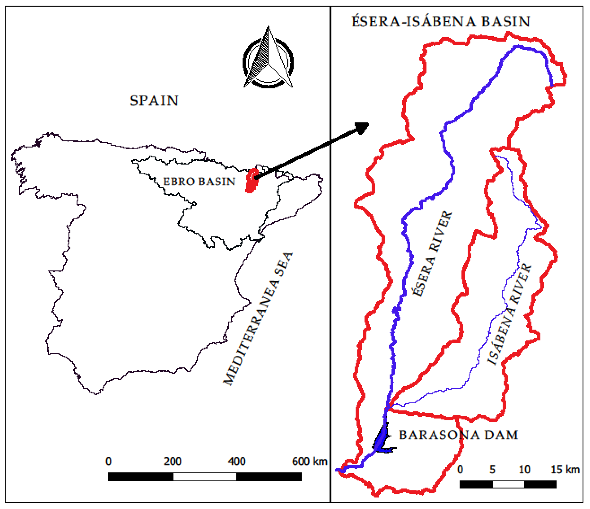
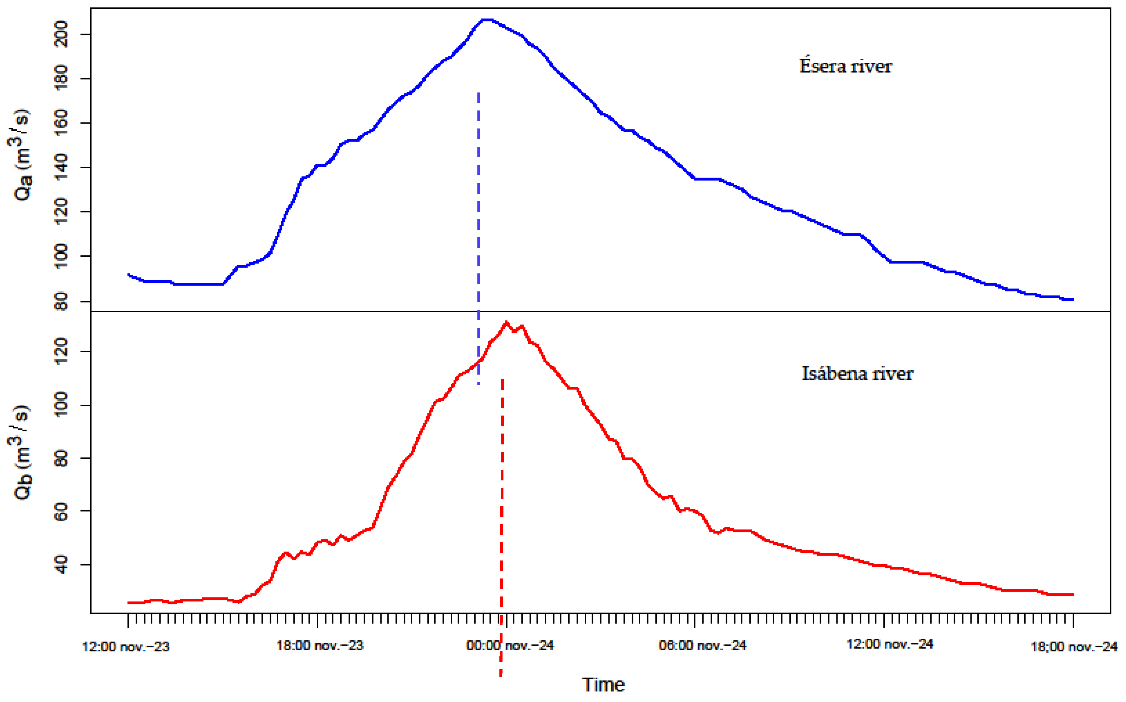
For the application of the formerly described methodology the following case study, located in the Ebro River basin (Spain) (Figure 1) was selected. More specifically, it consists of two mountain rivers: river Ésera and river Isábena, belonging to the basin of river Ebro. The areas of each catchment, are 893 km² and 426 km², respectively. Each of them has its own gauge station: Graus gauge station for river Ésera and Capella gauge station for Isábena. The ensemble of data was obtained, for both rivers, from the corresponding gauge stations, in such a way that 122 flood events were selected for the Esera River, and 157 for the Isábena River. All selected events match two conditions, i.e., present a rising limb with average slope over 20%, while the falling or recession limb presents a decay approximately exponential, following criteria in [4,46]. For illustration purposes, Figure 2 shows two observed hydrographs at river Esera and river Isábena for a given flood event.

Table 3. Basic hydrological descriptors for both river basins.

Variables	Ésera River	Isábena River
Area (km2)	983	446
Length (km)	97.32	66.13
Slope	0.030	0.034
Recorded Qmax (m3/s)	995	370
Recorded Vmax (m3)	147 × 4 × 106	61.7 × 106
Shape factor	0.27	0.24

summarizes some of the main hydrological characteristics of both river basins:

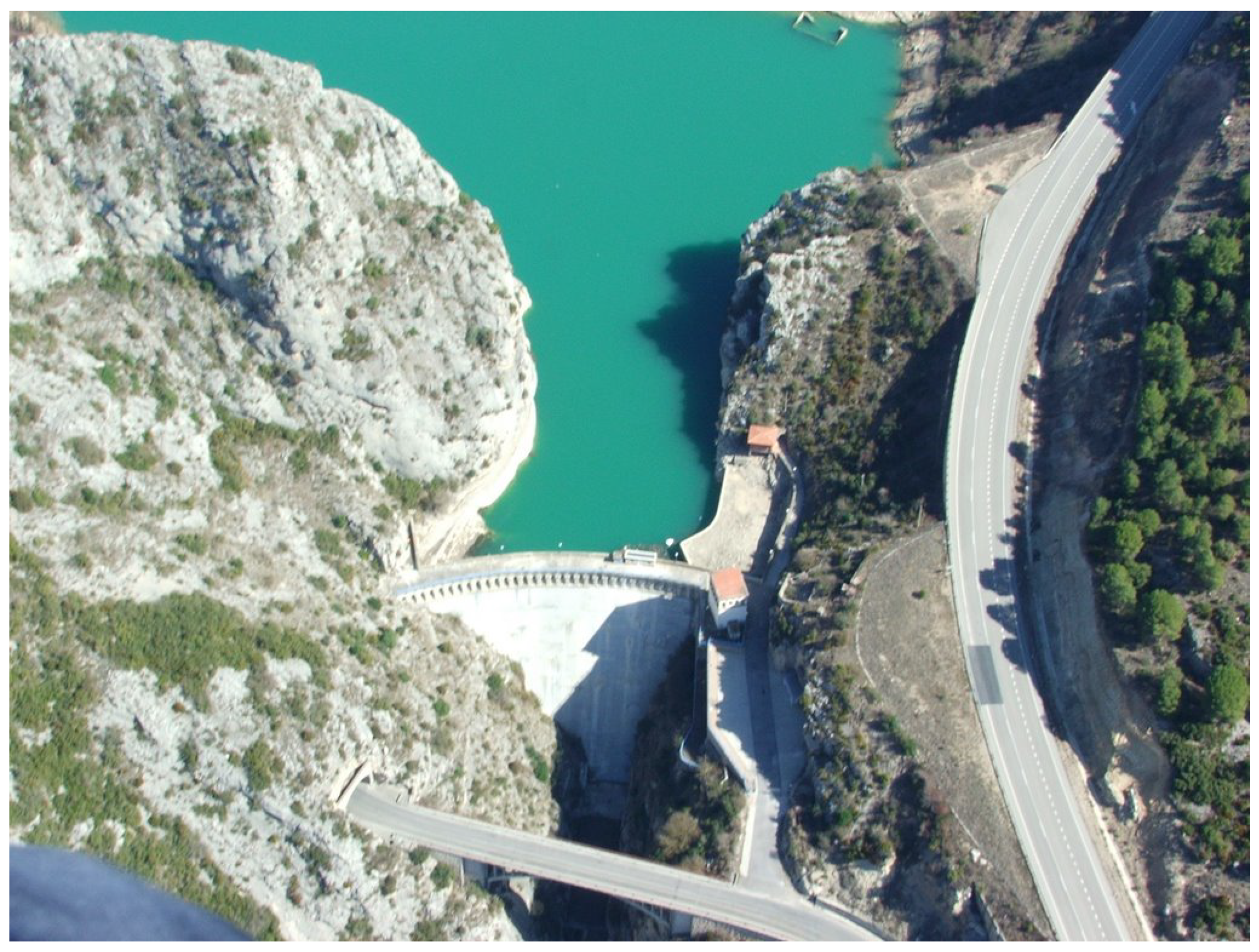
The Barasona reservoir is located downstream of the junction of both rivers. This reservoir is controlled by a 65 m high dam, with storage capacity of 85 × 10⁶ m³ (Figure 3). The dam is equipped with a side spillway controlled by 4 radial gates, Taintor type, whose dimensions are 10.0 × 4.75 m, providing a maximum total discharge capacity of 1500 m³/s.

The historical events that make up the sample belong to two periods, from the 1957–2000 period only the peak volume and volume are available but not the time lag between peaks. From the 2000–2017 period, detailed information of hydrograph time patterns Q(t) is available with a time resolution of Δt = 15 min (Figure 2).

3.1. Distributions Parameters Estimation

Following the methodology exposed in the former section, the adjustment of the marginal distributions of the two variables involved in the process (flow peak and volume of the hydrograph) is carried out. This procedure is applied for each of the gauge stations, corresponding to the rivers Ésera and Isábena.

Table 4. Flow registers basic statistics at gauge stations Graus and Capella.

Variables	Ésera River (Graus)		Isábena River (Capella)
	Qa	Va	Qb	Vb
No. hydrographs	122	122	157	157
Mean	229.16 m3/s	29.26 × 106 m3	85.80 m3/s	12.57 × 106 m3
Standard deviation	135.16 m3/s	23.70 m3	50.56 m3/s	11.72 m3
Minimum	60.90 m3/s	3.20 × 106 m3	6.50 m3/s	0.45 × 106 m3
Maximum	995.00 m3/s	147.40 × 106 m3	370.00 m3/s	61.70 × 106 m3
Skewness	2.48	2.36	2.51	1.67

summarizes some of the relevant statistics of the samples. Sub-index “a” stands for Ésera River and “b” stands for Isábena River

The statistical analysis of each variable has been developed employing three usual distribution functions: GEV, GPD and LPIII. Equations (11)–(13).

$$F\left(x\right)=e^{-{\left[1+\frac{\gamma \left(x-\alpha \right)}{\beta }\right]}^{-\frac{1}{\gamma }}}$$

(11)

$$F\left(x\right)=1-{\left[1+\frac{\gamma \left(x-\alpha \right)}{\beta }\right]}^{-\frac{1}{\gamma }}$$

(12)

$$f\left(x\right)=\frac{1}{ \left|\beta \right|\mathrm{x}\mathsf{\Gamma }\left(\gamma \right) } {\left[\frac{ln\left(x\right)-\alpha }{\beta }\right]}^{\gamma -1}{e}^{-\left[\frac{ln\left(x\right)-\alpha }{\beta }\right]}$$

(13)

where $\alpha$, $\beta ,$ and $\gamma$ are the location, scale, and shape parameters factors, respectively.

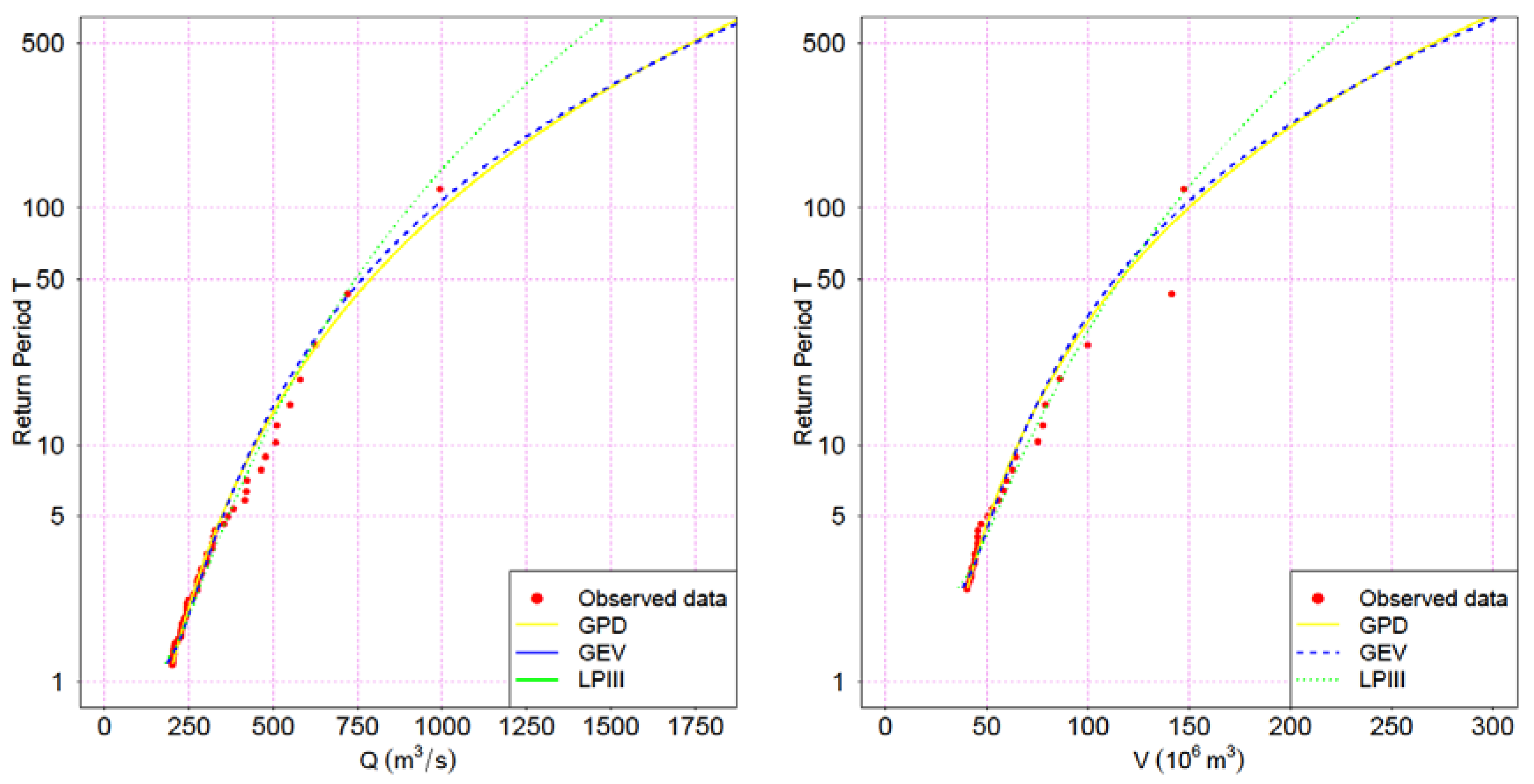
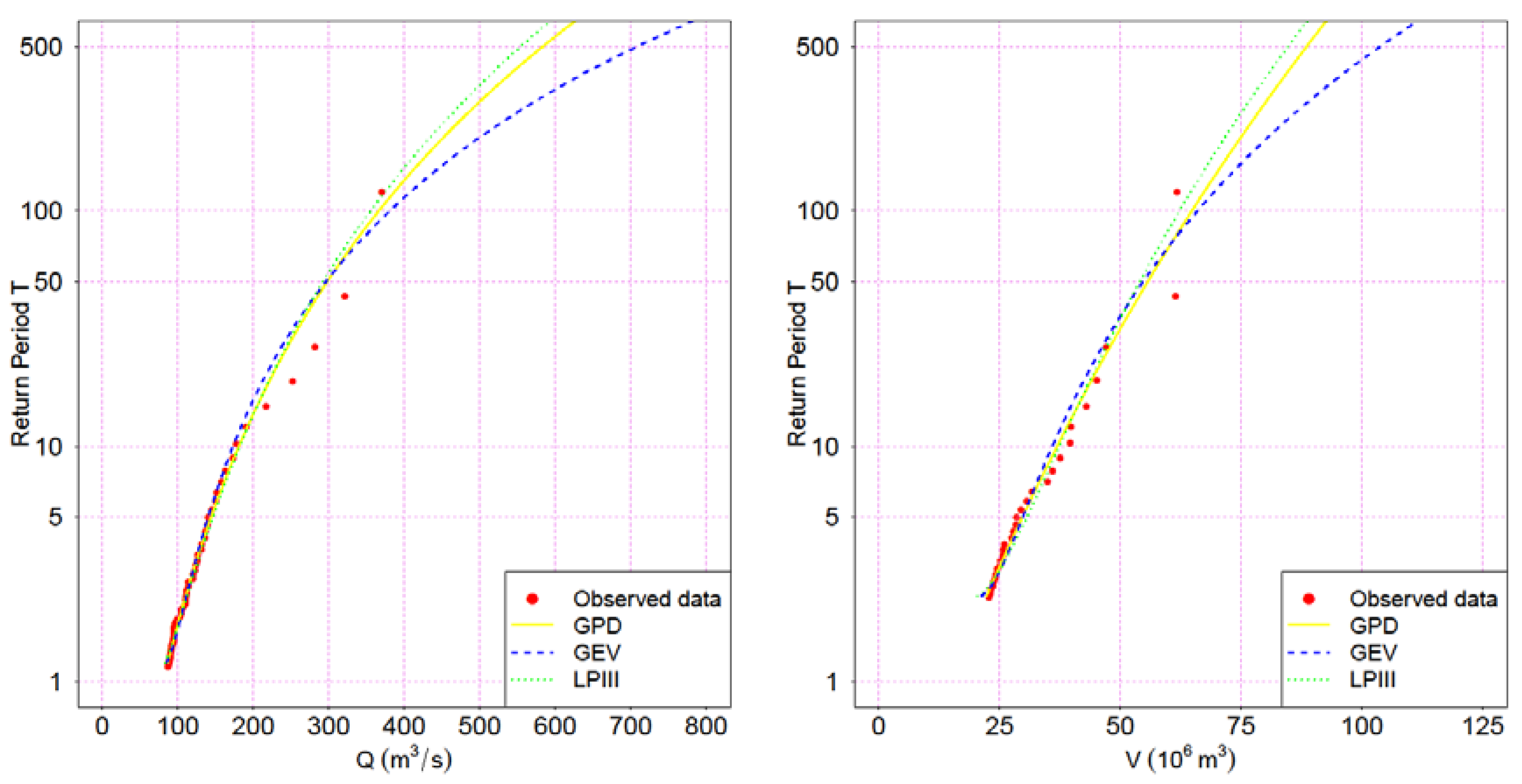
In all cases, the parameters were estimated with the PWM [24,25] method, as stated in Section 2.1. Subsequently, the goodness-of-fit test Anderson-Darling [23] was applied. Figure 4 and Figure 5 show the results for the different distribution functions tested. The estimated parameters are presented in

Table 5. Probability weighted moments (PWM) estimated parameters.

Distribution	GEV			LPIII			GPD
Parameters	Location	Scale	Shape	Location	Scale	Shape	Location	Scale	Shape
Q_Ésera	244.39	60.67	0.39	5.06	2.83	0.22	200	77.97	0.33
V_Ésera	47.44	10.44	0.44	3.44	2.77	0.22	40	13.34	0.38
Q_Isábena	102.56	20.41	0.43	4.35	1.81	0.25	85	32.42	0.27
V_Isábena	26.76	5.31	0.32	2.83	4.35	0.14	22	9.19	0.103

.

The Anderson–Darling test does not allow rejection of any of the distributions tested, while GPD has the theoretical support after employing POT method, as mentioned before. In terms of derived quantiles, and for all variables analyzed, LPIII yields to lower quantiles than the other two distributions for a given return period T.

GEV and GPD distributions are almost identical for Ésera River variables (differences of 1% for T = 250 and T = 500 years), which significant differences for large T in the case of Isábena River variables. For the sake of subsequent sections, the GPD distribution was adopted for all variables, except Q_a for which GEV was used.

Additionally, the time lag observed between the occurrences of peak flows in both rivers was analyzed.

The analyzed variable is t_a−b, defined as the existing time difference between the moments where the respective flow peaks occur at the respective gauge stations of Graus and Capella. This difference is quantified in hours. A positive value indicates that the flow peak happens first in river Ésera, while a negative value indicates the flood happens first in river Isábena.

Table 6. Empirical statistics of time lags between flow peaks.

Statistic	ta−b
No. observations	34
Mean	−1.40 h
Standard deviation	4.81 h
Minimum	−15.80 h
Maximum	15.00 h
Skewness	0.03

shows some relevant statistics of the sample. It should be noted that sample size for this empirical variable is now considerably reduced, as it is only extended to flood events registered with high resolution (Δt = 15 min). For the rest of the sample (period 1957–2000), the time patterns Q(t) and time lags between both river hydrograph peaks are unknown.

As explained before, the sample size for variable t_a−b is considerably reduced to support an extensive analysis for an optimal distribution function to adequately represent this variable. Nevertheless, the skewness (close to 0) suggests the hypothesis of the normal distribution function as a natural candidate, which was adopted in this case for the application presented herein.

3.2. Statistical Dependence among Variables

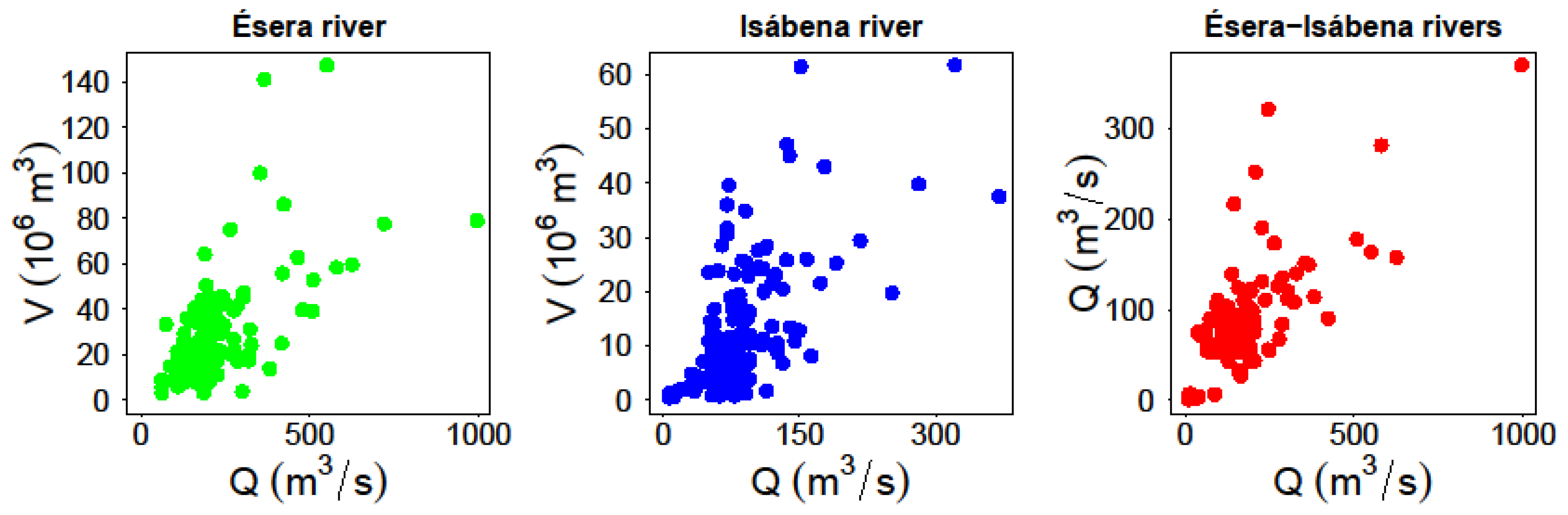
After analyzing each of the selected variables, the degree of empirical statistical dependence between pairs of variables is explored. Figure 6 shows the resulting clouds of points when different pairs of chosen variables are analyzed. For each case, indexes ρ-Sperman, τ-Kendall, and γ-Pearson were determined (

Table 7. γ-Pearson, τ Kendall, and ρ-Sperman statistics for selected pairs of variables.

	Estimated Values	p-Value
(Qa, Va)
ρ-Sperman	0.57	8.73 × 10−12
τ-Kendall	0.41	3.77 × 10−11
γ-Pearson	0.62	4.90 × 10−14
(Qb, Vb)
ρ-Sperman	0.57	1.04 × 10−14
τ-Kendall	0.40	7.47 × 10−14
γ-Pearson	0.62	2.20 × 10−16
(Qa, Qb)
ρ-Sperman	0.62	3.11 × 10−13
τ-Kendall	0.44	2.95 × 10−12
γ-Pearson	0.73	2.20 × 10−16

).

It must be noted that a significant correlation between the values of flow peak and volume of the hydrograph exists, of similar intensity for both rivers. That is, the analysis reveals that the hypothesis of statistically independent variables is not assumable and it becomes manifest that higher flow peaks come usually associated to important hydrograph volumes. From a hydrological point of view, this is the expected result, while it is also true that correlation indicators may vary between river basins and also according to the time of the year.

The developed analysis also reveals the existence of a certain degree of statistical dependence between the flow peaks of the different gauge stations. The occurrence of a flood event corresponds to a given meteorological situation that produces intense rain in the region, which generally affects both basins. While it is obvious that, depending on the location of the storm center and its spatial extension and movement, the magnitude of the flood generated in the rivers Ésera and Isábena can differ substantially.

Ultimately, these cannot be treated as statistically independent variables, reflecting the hydrological context determined by the closeness of both catchments and their spatial extension.

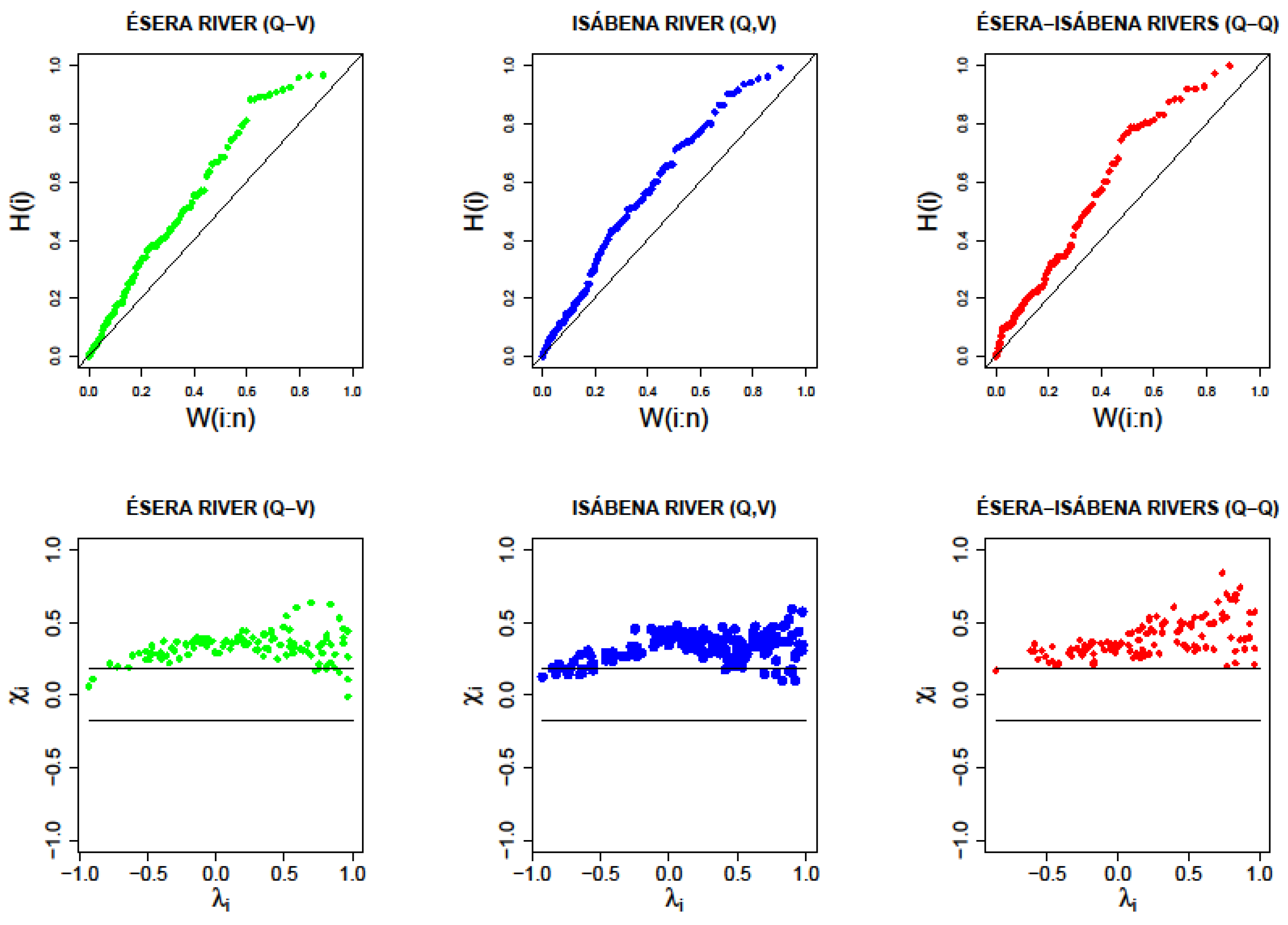
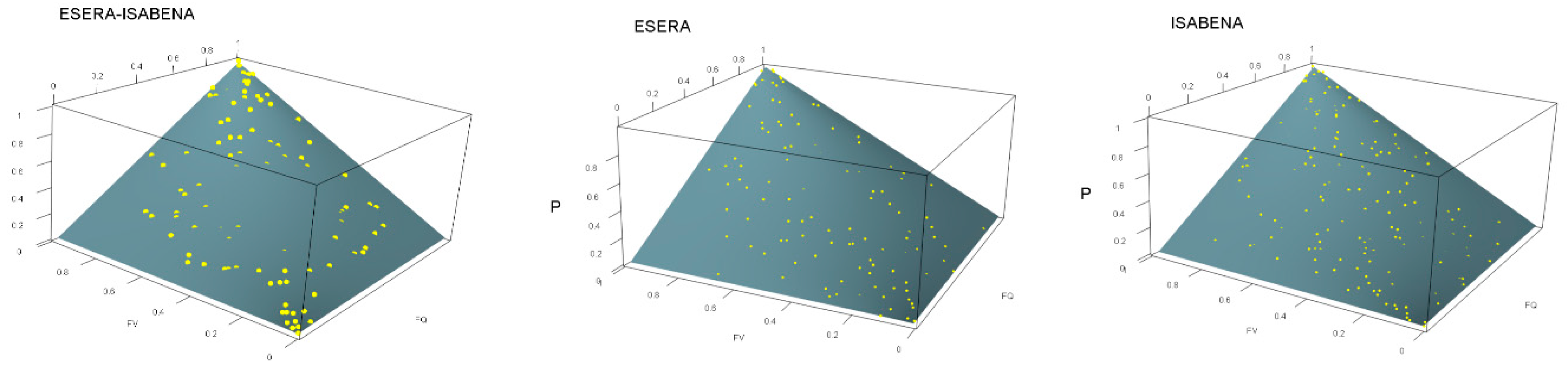
These conclusions are backed by the results of Figure 7, in which the developed chi-plot and k-plot are shown graphically. These indicators reveal the need to tackle the bivariate statistical analysis, and, therefore, justify the employment of copulas as a practical tool for a proper modelling of the structure of statistic dependence that has been empirically observed among variables, once the marginal distributions of the latter are known. It should be noted, though, that possible auto-correlations are not accounted for with the proposed scheme based on copulas, which might be relevant in case of clustering of extremes. Other more general approaches have been proposed in the literature, also preserving autocorrelations [47].

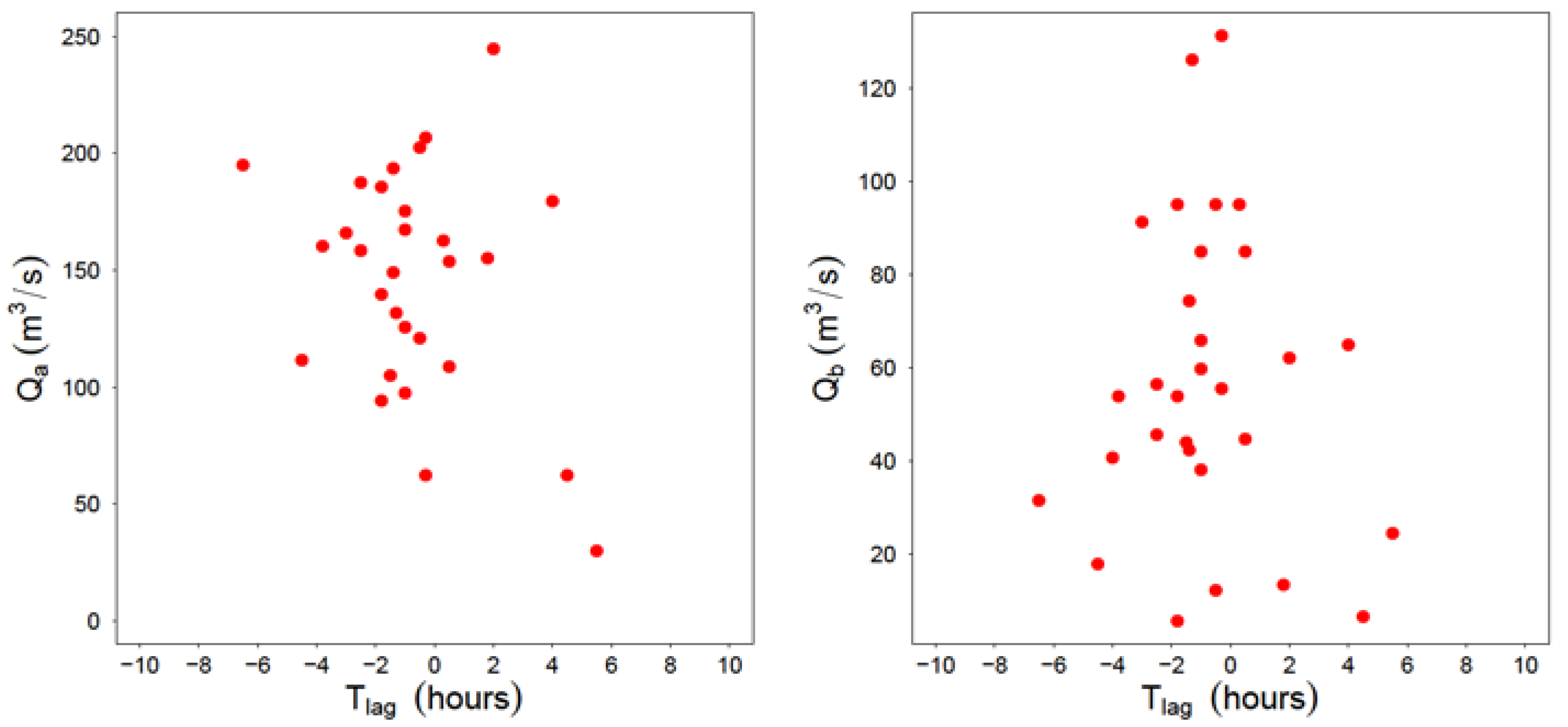
The method described in the former Section 2.3 is based on the hypothesis of independence of time lag between peaks t_a−b and the rest of variables (volume and flow peak in both gauge stations). The validity of this hypothesis has been empirically contrasted from the sample data. Figure 8 shows the graphic representation of flow peak vs time to peak for both rivers. Over these observed data, τ-Kendall and ρ-Sperman statistics have been estimated (

Table 8. τ-Kendall and ρ-Sperman statistics for selected pairs of variables.

Parameter	Value	p-Value
(Qa, ta−b)
ρ-Sperman	−0.19	0.12 > 0.05
τ-Kendall	−0.26	0.13 > 0.05
(Qb, ta−b)
ρ-Sperman	0.16	0.20 > 0.05
τ-Kendall	0.21	0.23 > 0.05

).

In both cases, values over 0.05 are found, which implies that the hypothesis of statistic independence between variables is assumable. This hypothesis is a necessary condition for the application of the synthetic hydrograph generation method as exposed in Section 2.3.

In hydrological terms, the results are an indication of a casuistic of floods produced for incoming rain fronts in the river basins from different directions. That is to say, it corresponds to a range of synoptic situations which produce the advancement or delay of runoff, indistinctly in one catchment or the other. In any case, it must be noted that the average estimated value of t_a−b is −1.4 h. In other words, most frequently, peaks tend to happen earlier in the Graus gauge station (river Ésera).

3.3. Copula Selection

Once the marginals have been chosen, the selection of the copulas for each pair of variables, (Q_a, Q_b) (Q_a, V_a) and (Q_b, V_b) must be done. Since focus lies on maximum hydrographs for high return periods (T > 100), the family of extreme value copulas is chosen. Within this group, the Gumbel, Galambos and H–R are the most noticeable ones; with their expressions and characteristic values being shown in Table 1.

The characteristic parameter of the copula was obtained by means of three methods of statistic inference:

• τ-Kendall inversion;
• ρ-Sperman inversion;
• Maximum pseudo-likelihood

Table 9. Estimated copula values for different methods (Q_a, V_a).

Ésera River (Qa, Va)
Copula	Estimation Method	${\mathit{\theta }}_{\mathit{n}}$	${\mathit{S}}_{\mathit{n}}$	p-Value
Gumbel	τ-Kendall inversion	2.021	0.0177	0.19
	ρ-Sperman inversion	2.052	0.0224	0.17
	MPL	1.678	0.0096	0.30
Galambos	τ-Kendall inversion	0.962	0.0067	0.73
	ρ-de Sperman	0.954	0.0075	0.74
	MPL	0.972	0.0061	0.47
H–R	τ-Kendall	1.425	0.0048	0.83
	ρ-Sperman	1.411	0.0061	0.80
	MPL	1.472	0.0041	0.54

,

Table 10. Estimated copula values for different methods (Q_b, V_b).

Isábena River (Qb, Vb)
Cópula	Estimation Method	${\mathit{\theta }}_{\mathit{n}}$	${\mathit{S}}_{\mathit{n}}$	p-Value
Gumbel	τ-Kendall inversion	1.676	0.0055	0.83
	ρ-Sperman inversion	1.677	0.0055	0.84
	MPL	1.665	0.0060	0.58
Galambos	τ-Kendall inversion	0.955	0.0042	0.88
	ρ-Sperman inversion	0.951	0.0043	0.90
	MPL	0.950	0.0043	0.62
H–R	τ-Kendall inversion	1.418	0.0034	0.91
	ρ-Sperman inversion	1.407	0.0039	0.90
	MPL	1.425	0.0034	0.65

and

Table 11. Estimated copula values for different methods (Q_a, Q_b).

Ésera-Isábena Rivers (Qa, Qb)
Copula	Estimation Method	${\mathit{\theta }}_{\mathit{n}}$	${\mathit{S}}_{\mathit{n}}$	p-Value
Gumbel	τ-Kendall inversion	1.796	0.0095	0.57
	ρ-Sperman inversion	1.797	0.0094	0.62
	MPL	1.909	0.0014	0.89
Galambos	τ-Kendall inversion	1.079	0.0097	0.56
	ρ-Sperman inversion	1.072	0.0110	0.54
	MPL	1.193	0.0017	0.78
H–R	τ-Kendall inversion	1.563	0.0106	0.48
	ρ-Sperman inversion	1.548	0.0132	0.47
	MPL	1.690	0.0024	0.64

summarize the obtained results. These tables detail, for each case, the adopted inference method, the value of the copula, the p-value, as well as the Cramer-von Mises statistic, proposed by the authors of [29], Equation (2). In each of the tables, the best obtained statistics are shown in bold.

As it can be observed, the copula that shows the best behavior for the flow peak in both rivers is the Gumbel one, whereas for the relation (Q, V) in rivers Ésera and Isábena it is the H–R one.

Applying what was exposed in Section 2.2.4 to the selected copulas, the dependence coefficient of the upper tail of the distribution is analyzed, comparing the empirical and the theoretical values of the statistic ${\lambda }_U$ (

Table 12. ${\lambda }_U^C\left(\theta \right)$ Estimated values.

Copula	$\mathit{\theta }$	$\mathit{\theta }$	$\mathit{\theta }$	${\mathit{\lambda }}_{\mathit{U}}^{\mathit{C}}\left(\mathit{\theta }\right)$	${\mathit{\lambda }}_{\mathit{U}}^{\mathit{C}}$	${\mathit{\lambda }}_{\mathit{U}}^{\mathit{C}}$	${\mathit{\lambda }}_{\mathit{U}}^{\mathit{C}}$
	(Qa, Va)	(Qb, Vb)	(Qa, Qb)		(Qa, Va)	(Qb, Vb)	(Qa, Qb)
Gumbel	1.678	1.677	1.909	$2-2^{\frac{1}{\theta }}$	0.488	0.488	0.562
Galambos	0.954	0.951	1.193	$2^{\frac{-1}{\theta }}$	0.483	0.482	0.559
H–R	1.425	1.418	1.690	$2-2·\Phi \left\{\frac{1}{\theta }\right\}$	0.482	0.481	0.535

and

Table 13. Estimated values for ${\widehat{\lambda }}_U^{CFG}$.

${\widehat{\mathit{\lambda }}}_{\mathit{U}}^{\mathit{C}\mathit{F}\mathit{G}}$	Sample
0.485	$\theta$(Qa, Va)
0.476	$\theta$(Qb, Vb)
0.570	θ(Qa, Qb)

).

As it can be observed, theoretical and empirical values are very similar, indicating a satisfactory behavior of the right upper tail of the distribution. The values highlighted in bold are the ones that fit the empirical estimators of the sample. According to this, it can be concluded that the Gumbel copula is the best suited one to represent the pairs (Q_a, Q_b), Galambos is the one that best represents the pairs (Q_a, V_a), and finally H–R is the best suited for (Q_b, V_b).

3.4. Monte Carlo Simulation of Flood Peaks and Volumes

A long synthetic series of 50,000 pairs (Q_a, Q_b), (Q_a, V_a), (Q_b, V_b) has been generated, following the scheme explained in Section 2.3, by means of a Monte Carlo simulation. That is, through random number generation and the Gumbel copula (Q_a, Q_b), synthetic values of respective peak flows in both rivers are generated. Synthetic values of hydrograph volumes are then derived using H–R copulas (Q_a, V_a) and (Q_b, V_b).

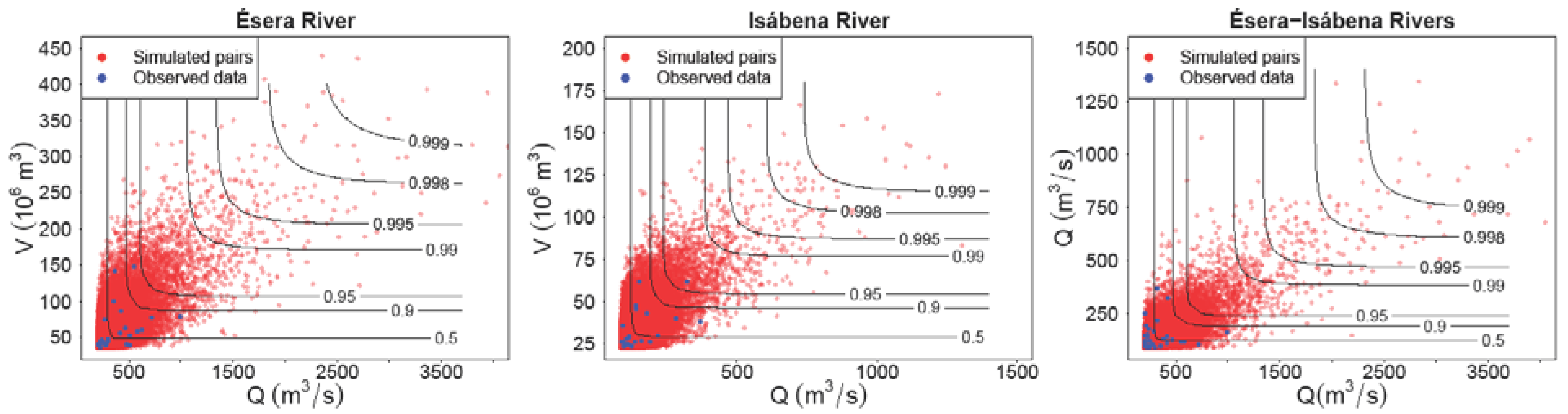
In the Figure 9, the Gumbel’s, Galambos and H–R 2-Copula values are plotted, and compared with the corresponding empirical 2-Copula function. The agreement between the data and the model is objectively checked via a standard test, explained below.

Figure 10 shows the results of the simulation for both the synthetic values and the points corresponding to the real hydrographs analyzed. In addition, the thresholds or quantiles corresponding to different probability levels are indicated with a continuous line.

3.5. Synthetic Generation of Hydrographs

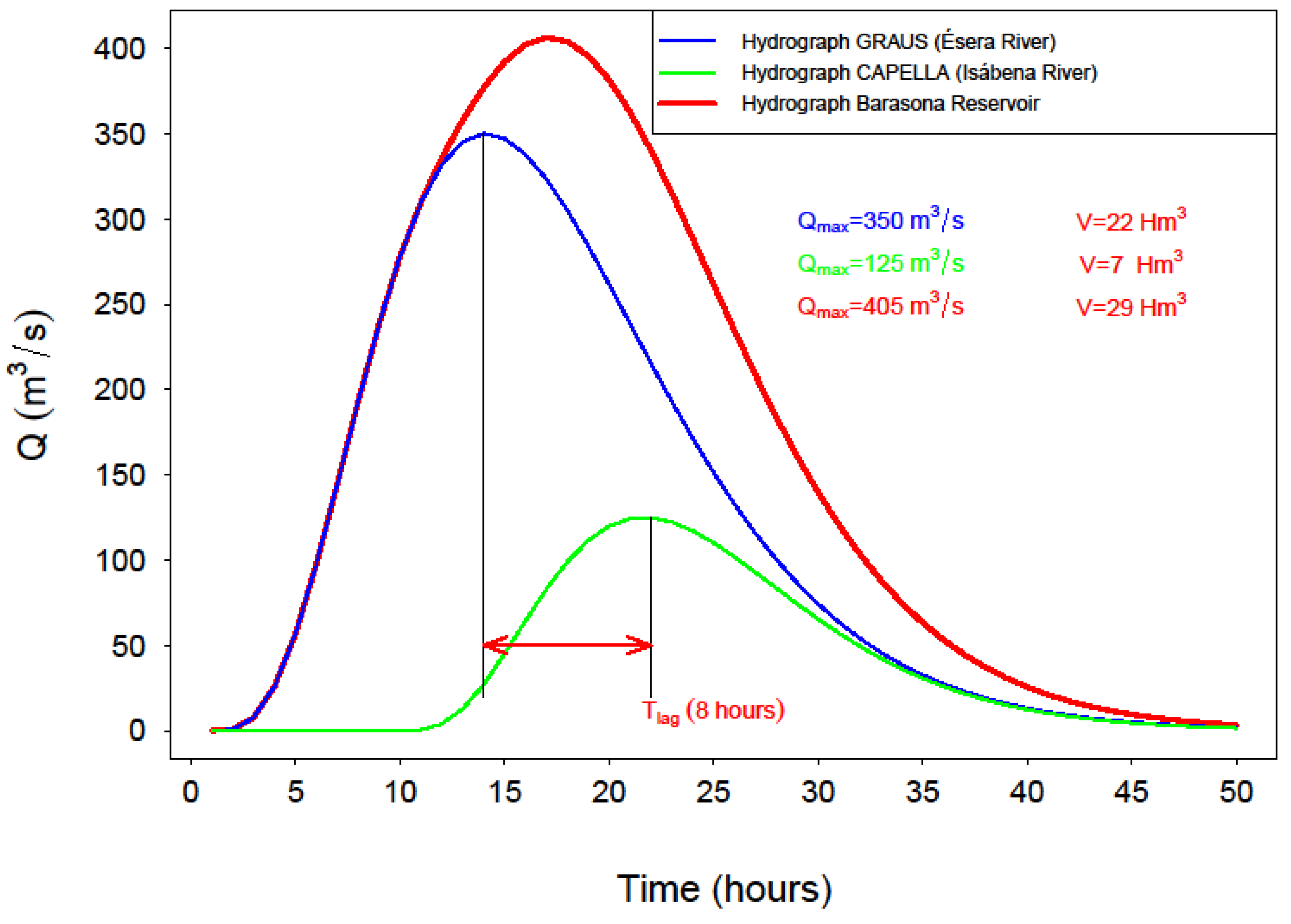
Every one of the synthetic pairs (Q_a, V_a), (Q_b, V_b) generated as explained in Section 3.4, is assigned to a gamma-type time pattern Q(t), preserving both synthetic values of flow peak and hydrograph volume. To do so, the procedure explained in Section 2.3 is applied, allowing one to proceed with the hydrological sum of both synthetic hydrographs in time. This last step is illustrated in Figure 11, where it can be seen that there exists a time lag between hydrographs peaks, which is also synthetically generated using the normal distribution presented in Section 3.1. The time step used to represent synthetic hydrographs is Δt = 15 min.

The result of applying this method is a sample of synthetic hydrographs downstream of the junction of rivers Ésera and Isábena, each of them defined by its flow peak, volume, and time pattern.

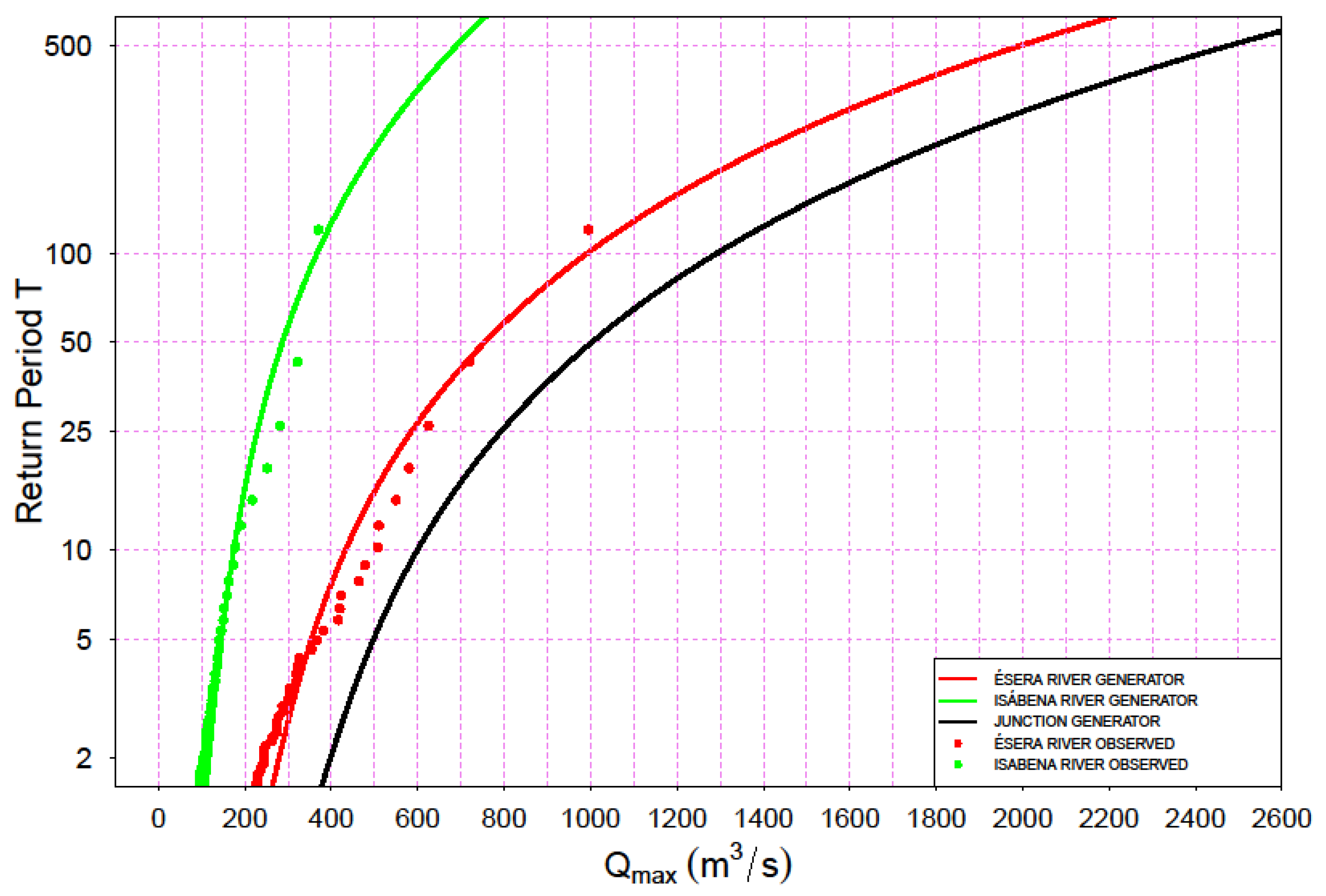
The final statistical analysis of the synthetic samples is shown in Figure 12. This figure shows the quantiles of maximum flows, derived from the synthetic sample in both rivers, as well as downstream of the junction. A simple formula for the plotting position was employed (Equation (14)) to represent the empirical frequency. In this formula, r is the order of each of the values and c is a coefficient. In this case, c = 0.44 (Gringorten). In addition, the plotting positions corresponding to the observed values for flow peaks are also shown.

$$\widehat{F}\left(x_{\left|r\right|}\right)=\frac{r-c}{n+1-2c}$$

(14)

The resulting estimations after the described method allow to estimate quantiles of high return period, as summed up in

Table 14. Estimated flow peaks (m³/s) for different return periods at Graus (Ésera), Capella (Isábena), and Barasona reservoir.

Return Period (years)	10	25	50	100	500
Ésera River	432	585	754	993	1994
Isábena River	174	228	286	367	689
Barasona reservoir	559	791	1002	1293	2477

.

4. Discussion and Conclusions

As already stated in Section 3, the available information for flood hydrographs is very limited for the Barasona reservoir study, whereas the gauge stations of both confluent rivers provide reliable and representative information for each of them. The analysis carried out in the present research makes it possible to increase the feasibility and soundness of the quantiles estimation for flow peak and volume of the hydrograph at the reservoir entrance, which is located downstream of the two rivers junction.

This analysis considers the observed statistical dependence between the flow peaks for rivers Ésera and Isábena, as well as the existing statistical dependence between flow peak and volume for each of the partial hydrographs. In order to do this, three copulas are introduced, which allow a bivariate analysis of pairs (Q_a, Q_b); (Q_a, V_a) and (Q_b, V_b). Once these analyses have been concluded, the generation of synthetic events in both gauge stations becomes feasible, defining them in terms of flow peak and volume and respecting the empirically observed structure of statistical dependence. Also, the introduction of a theoretical time pattern based on Nash hydrograph enables the analytical definition of Q(t) for each synthetic event. Time lag between flow peaks for partial hydrographs is dealt with as an independent random variable, simplifying the operation to obtain the resulting synthetic hydrograph at the entrance of Barasona reservoir.

Consequently, the research presented herein does not introduce new specific methodologies, as it mainly combines effectively several well-known techniques, i.e., copula techniques, classical distribution functions, and usual procedures for Monte Carlo synthetic generation.

It represents, though, an interesting modelling approach which is essentially conceived for the practical case in flood hydrology when the river section of interest is ungauged, being located downstream a junction of two tributaries (both of them with available flow records). The specific hypotheses employed herein are very much conditioned by the length and nature of the available information in the particular case study. Obviously, there are other modelling approaches that could be appropriate and applicable for this case study. The one presented herein makes intense use of copula theory successfully, providing an efficient and useful modelling framework in an engineering hydrology context.

In particular, it makes an efficient use of incomplete and non-homogeneous hydrological data, providing the required answers to certain practical flood managing problems, as well as improving reliability of high return period quantiles estimation.

The modelling strategy is oriented towards the improvement of hydrological risk assessment in large dams, providing the appropriate hydrological inputs [48,49,50].

The results obtained allow further analysis of dam routing under different initial reservoir freeboards and different strategies concerning operations with gate-controlled spillways. Particularly, it becomes interesting to translate input hydrological variables (associated to the corresponding return period), into dam operation variables. For instance, variables such as the maximum level reached in the reservoir during the dam routing process, overtopping risk, maximum spilled flows during the dam routing or required freeboard to limit overtopping risk with a given probability value.

These ensuing variables become increasingly more interesting from a point of view of decision making for optimal dam operation.

References

- Xiao:, Y.; Guo, S.; Liu, P.; Yan, B.; Chen, L. Design Flood Hydrograph Based on Multicharacteristic Synthesis Index Method. J. Hydrol. Eng. 2009, 14, 1359–1364. [Google Scholar] [CrossRef]
- Rosbjerg, D.; Blöschl, G.; Burn, D.; Castellarin, A.; Croke, B.; Di Baldassare, G.; Iacobellis, V.; Kjeldsen, T.; Kuczera, G.; Merz, R.; et al. Prediction of floods in ungauged basins. In Runoff Prediction in Ungauged Basins: Synthesis Across Processes, Places and Scales; Cambridge University Press: Cambridge, UK, 2013; pp. 189–226. [Google Scholar]
- Salvadori, G.; De Michele, C. Frequency analysis via copulas: Theoretical aspects and applications to hydrological events. Water Resour. Res. 2004, 40, 1–17. [Google Scholar] [CrossRef]
- Mediero, L.; Jiménez-Álvarez, A.; Garrote, L. Design flood hydrographs from the relationship between flood peak and volume. Hydrol. Earth Syst. Sci. 2010, 14, 2495–2505. [Google Scholar] [CrossRef] [Green Version]
- Requena, A.I.; Mediero, L.; Garrote, L. A bivariate return period based on copulas for hydrologic dam design: accounting for reservoir routing in risk estimation. Hydrol. Earth Syst. Sci. 2013, 17, 3023–3038. [Google Scholar] [CrossRef] [Green Version]
- De Michele, C.; Salvadori, G.; Canossi, M.; Petaccia, A.; Rosso, R. Bivariate Statistical Approach to Check Adequacy of Dam Spillway. J. Hydrol. Eng. 2005, 10, 50–57. [Google Scholar] [CrossRef]
- Sklar, M. Sklar. Fonctions de répartition à n dimensions et leurs marges; l’Institut de Statistique de L’Universite de Paris: Paris, France, 1959; Volume 8, pp. 229–231. [Google Scholar]
- Favre, A.-C.; El Adlouni, S.; Perreault, L.; Thiémonge, N.; Bobée, B. Multivariate hydrological frequency analysis using copulas. Water Resour. Res. 2004, 40, 1–12. [Google Scholar] [CrossRef]
- Zhang, L.; Singh, V.P. Bivariate flood frequency analysis using the copula method. J. Hydrol. Eng. 2006, 11, 150–164. [Google Scholar] [CrossRef]
- Klein, B.; Pahlow, M.; Hundecha, Y.; Schumann, A. Probability analysis of hydrological loads for the design of flood control systems using copulas. J. Hydrol. Eng. 2010, 15, 360–369. [Google Scholar] [CrossRef]
- Papaioannou, G.; Kohnová, S.; Bacigál, T.; Szolgay, J.; Hlavčová, K.; Loukas, A. Joint modelling of flood peaks and volumes: A copula application for the Danube River. J. Hydrol. Hydromech. 2016, 64, 382–392. [Google Scholar] [CrossRef] [Green Version]
- Afshar, M.H.; Sorman, A.U.; Yilmaz, M.T. Conditional Copula-Based Spatial–Temporal Drought Characteristics Analysis—A Case Study over Turkey. Water 2016, 8, 426. [Google Scholar] [CrossRef]
- De Luca, D.L.; Biondi, D. Bivariate Return Period for Design Hyetograph and Relationship with T-Year Design Flood Peak. Water 2017, 9, 673. [Google Scholar] [CrossRef]
- Aranda Domingo, J.A. Estimación de la Probabilidad de Sobrevertido y Caudales Máximos Aguas Abajo de Presas de Embalse. Efecto del Grado de Llenado Inicial. Ph.D. Thesis, Technical University of Valencia, Valencia, Spain, March 2014. [Google Scholar]
- Prohaska, S.; Ilic, A.; Majkic, B. Multiple-coincidence of flood waves on the main river and its tributaries. In Iop Conference Series: Earth and Environmental Science; IOP Science: Bristol, UK, 2008; Volume 4, pp. 1088–1755. [Google Scholar]
- Prohaska, S.; Ilic, A. Coincidence of Flood Flow of the Danube River and its Tributaries. In Hydrological processes of the Danube River Basin; Brilly, M., Ed.; Springer: Dordrecht, The Netherlands, 2010; pp. 175–226. [Google Scholar]
- Prohaska, S.; Ilic, A.; Tripkovic, V. Methodology for Assessing Multiple-Coincidence of Flood Wave Peaks in Complex River Systems. Water Res Manag. 2012, 2, 45–60. [Google Scholar]
- Chen, L.; Singh, V.P.; Guo, S.L.; Hao, Z.C.; Li, T.Y. Flood Coincidence Risk Analysis Using Multivariate Copula Functions. J. Hydrol. Eng. 2012, 17, 742–755. [Google Scholar] [CrossRef]
- Chen, L.; Singh, V.P.; Guo, S.L. Measure of Correlation between River Flows Using the Copula-Entropy Method. J. Hydrol. Eng. 2013, 18, 1591–1606. [Google Scholar] [CrossRef]
- Bender, J.; Wahl, T.; Müller, A.; Jensen, J. A multivariate design framework for river confluences. Hydrol. Sci. J. 2016, 61, 471–482. [Google Scholar] [CrossRef]
- Campos-Aranda, D.F. Empirical approach to the bivariate solution for flood design in reservoirs without hydrometrical data. Agrociencia 2010, 44, 735–752. [Google Scholar]
- Balkema, A.; de Haan, L. Residual Life Time at Great Age. Ann. Probab. 1974, 2, 792–804. [Google Scholar] [CrossRef]
- Ferreira, A.; de Haan, L. On the block maxima method in extreme value theory: PWM estimators. Ann. Probab. 2015, 43, 276–298. [Google Scholar] [CrossRef] [Green Version]
- Hosking, J.; Wallis, J.; Wood, E. Estimation of the Generalized Extreme-Value Distribution by the Method of Probability-Weighted Moments. Technometrics 1985, 27, 251–261. [Google Scholar] [CrossRef]
- Dupuis, D.J. Estimating the probability of obtaining nonfeasible parameter estimates of the generalized pareto distribution. J. Stat. Comput. Simul. 1996, 54, 197–209. [Google Scholar] [CrossRef]
- Genest, C.; Favre, A.-C. Everything you always wanted to know about copula modeling but were afraid to ask. J. Hydrol. Eng. 2007, 12, 347–368. [Google Scholar] [CrossRef]
- Dupuis D., J. Using Copulas in Hydrology: Benefits, Cautions, and Issues. J. Hydrol. Eng. 2007, 12, 381–393. [Google Scholar] [CrossRef]
- Gudendorf, G.; Segers, J. Extreme-Value copulas. In Proceedings of the Workshop Held in Warsaw, Warsaw, Poland, 25–26 September 2009; Springer, Berlin, Germany, Durante, F., Haerdle, W., Jaworski, P., Rychlik, T., Eds.; 2010. [Google Scholar]
- Joe, H.; Xu, J.J. The Estimation Method of Inference Functions for Margins for Multivariate Models; Technical Report 166; The University of British Colombia: Vancouver, CA, Canada, 1996. [Google Scholar]
- Kim, G.; Silvapulle, M.J.; Silvapulle, P. Comparison of semiparametric and parametric methods for estimating copulas. Comput. Stat. Data Anal. 2007, 51, 2836–2850. [Google Scholar] [CrossRef]
- Genest, C.; Rémillard, B. Validity of the parametric bootstrap for goodness-of-fit testing in semiparametric models. Annales de l’I.H.P. Probabilités et Statistiques 2008, 44, 1096–1127. [Google Scholar] [CrossRef]
- Genest, C.; Kojadinovic, I.; Nešlehová, J.; Yan, J. A goodness-of-fit test for bivariate extreme-value copulas. Bernoulli 2011, 17, 253–275. [Google Scholar] [CrossRef]
- Serinaldi, F. Analysis of inter-gauge dependence by Kendall’s τ K, upper tail dependence coefficient, and 2-copulas with application to rainfall fields. Stoch. Environ. Res. Risk A. 2008, 22, 671–688. [Google Scholar] [CrossRef]
- Schmidt, R. Tail dependence. In STATISTICAL Tools in Finance and Insurance, 2nd ed.; Cizek, P., Härdle, W., Weron, R., Eds.; Springer: New York, NY, USA, 2005; pp. 65–84. [Google Scholar]
- Schmidt, R.; Stadtmüller, U. Non-parametric estimation of tail dependence. Scand. J. Stat. 2006, 33, 307–335. [Google Scholar] [CrossRef]
- Frahm, G.; Junker, M.; Schmidt, R. Estimating the tail-dependence coefficient: Properties and pitfalls. Insur. Math. Econ. 2005, 37, 80–100. [Google Scholar] [CrossRef]
- Schmidt, R. Dependencies of Extreme Events in Finance: Modelling, Statistics, and Data Analysis. Ph.D Thesis, University of Ulm, Ulm, Germany, 2003. [Google Scholar]
- Capéraà, P.; Fougères, A.-L.; Genest, C. A nonparametric estimation procedure for bivariate extreme value copulas. Biometrika 1997, 84, 567–577. [Google Scholar] [CrossRef]
- Schulte, M.; Schumann, A. Evaluation of Flood Coincidence and Retention Measures by Copulas. Wasserwirtschaft 2016, 106, 81–87. [Google Scholar]
- Zhang, N.; Lv, L.L.; Jiang, H.; Huang, K. Flood coincidence probability analysis for the middle and low Weihe River and its tributaries based on the LHS method. In Advances in Earth and Environmental Sciences; Yang, Y., Ed.; WIT Press: Ashurst, UK, 2014. [Google Scholar]
- Devroye, L. Non-Uniform Random Variate Generation; Springer-Verlag: New York, NY, USA, 1986. [Google Scholar]
- Johnson, M.E. Multivariate Statistical Simulation; J. Wiley Sons: New York, NY, USA, 1987. [Google Scholar]
- Nash, J.E. The form of instantaneous unit hydrograph. IAHS Publ. 1957, 45, 114–121. [Google Scholar]
- Bras, R.L. Hydrology: An Introduction to Hydrologic Science; Addison-Wesley: Boston, MA, USA, 1990; p. 447. [Google Scholar]
- Croley, T.E. Gamma synthetic hydrographs. J. Hydrol. 1980, 47, 26–49. [Google Scholar] [CrossRef]
- Cunnane, C. A note on the Poisson assumption in partial duration series models. Water Resour. Res. 1979, 15, 489–494. [Google Scholar] [CrossRef]
- Papalexiou, S.M. Unified theory for stochastic modelling of hydroclimatic processes: Preserving marginal distributions, correlation structures, and intermittency. Adv. Water Resour. 2018, 115, 234–252. [Google Scholar] [CrossRef]
- Chen, Y.; Lin, P. The Total Risk Analysis of Le Dams under Flood Hazards. Water 2018, 10, 140. [Google Scholar] [CrossRef]
- Karmaker, T.; Dutta, S. Generation of synthetic seasonal hydrographs for a large river basin. J. Hydrol. 2010, 381, 287–296. [Google Scholar] [CrossRef]
- Gioia, A. Reservoir Routing on Double-Peak Design Flood. Water 2016, 8, 533. [Google Scholar] [CrossRef]
Figure 1.
Geographical location of rivers Ésera and Isábena.
Figure 2.
Observed hydrographs for the 23 January 2016 flood event.
Figure 3.
View of the Barasona dam, downstream of the junction of both rivers.
Figure 4.
Distribution functions for flow peak and hydrograph volume (Ésera River).
Figure 5.
Distribution functions for flow peak and hydrograph volume (Isábena River).
Figure 6.
Correlation analysis between relevant variables.
Figure 7.
K-plots and chi-plots for the selected samples.
Figure 8.
Maximum flow peaks vs. time lag between both river hydrographs.
Figure 9.
Comparison between empirical and theoretical copula.
Figure 10.
Scatter plot of 50,000 values generated from the copulas fitted.
Figure 11.
Example of synthetic generated hydrographs.
Figure 12.
Empirical plotting positions and resulting distributions after the Monte Carlo simulation.