A Robust and Transferable Model for the Prediction of Flood Losses on Household Contents
by
 , ,
, ,
Markus Mosimann
1,2,3,* ,
,
Linda Frossard
1,2,3,
Margreth Keiler
1,2,
Rolf Weingartner
1,2,3 and
Andreas Paul Zischg
1,2,3 1
Institute of Geography, University of Bern, Hallerstrasse 12, CH-3012 Bern, Switzerland
2
Mobiliar Lab for Natural Risks, University of Bern, Hallerstrasse 12, CH-3012 Bern, Switzerland
3
Oeschger Centre for Climate Change Research, University of Bern, Falkenplatz 16, CH-3012 Bern, Switzerland
*
Author to whom correspondence should be addressed.
Water 2018, 10(11), 1596; https://doi.org/10.3390/w10111596
Submission received: 3 October 2018
/
Revised: 25 October 2018
/
Accepted: 1 November 2018
/
Published: 7 November 2018
(This article belongs to the Section Water Resources Management, Policy and Governance)
Abstract
:Beside the flood hazard analysis, a comprehensive flood risk assessment requires the analysis of the exposure of values at risk and their vulnerability. Currently, the main focus of such analysis is on losses on building structure. However, loss on household contents accounts for up to 30% of the total losses on buildings due to floods. Based on insurance claim records, we developed and (cross-)validated two functions. The models based on linear regressions estimate the monetary loss and the degree of loss of household contents by the monetary and degree of loss for building structure, respectively. The main focus herein is to develop functions which provide robustness in prediction and transferability to other regions. Both models generate appropriate results with a comparative advantage of the relative over the absolute loss model. Our results indicate that the ratio of household content to building structure loss is decreasing relatively in regions with comparatively high losses or degrees of loss. A detailed examination of the model residuals, shows that the Box-Cox transformation works well to accurately fit a standard regression model to general right-skewed loss data as the transformed data meet the assumptions of a regression model.
1. Introduction
Floods are one of the most frequent natural hazards worldwide, affecting more people than any other hazard and being responsible for one third of the global expected annual average loss of USD 314 billion [1]. Therefore, the assessment of flood risk (defined by hazard, exposure and vulnerability [2]) and thus the analysis of losses due to floods constitutes a substantial public interest. Several studies assess flood risk on a global scale coping with low-resolution data [3,4,5] to for instance make projections to future flood risk scenarios [6] or to find regions that should be prioritized for river-flood protection investments [7]. Floods are also a topical issue on national (CH), regional (cantons) and local (municipalities) scale. Based on a database from 1946 to 2015, flood ranks third in the list of most fatal catastrophes related to natural hazards in Switzerland [8]. According to Swiss Re [9], floods accounted for 71% of the total loss due to natural hazards in Switzerland over the period 1973 to 2011. Compared to windstorm (15%), hailstorm (11%) and other perils (3%), this indicates the relevance of national, regional and even local flood risk assessment. The destructive potential was also shown in August 2005, when floods and debris flows in Switzerland led to financial losses of more than CHF 3 billion (roughly EUR 2 billion) [10].
However, on local scale, namely for Swiss municipalities, the resolution used in the global studies mentioned is to coarse to also consider creaks and mesoscale catchments representatively. The availability of spatially and temporally high resolved flood models and the possibility to develop flood scenarios lead to new perspectives in detecting regions or even single buildings with a high loss potential. Especially, flood losses are increasingly estimated at the scale of single buildings [11,12,13,14,15,16]. Because inundations rarely lead to a total destruction of buildings, e.g., Papathoma-Köhle et al. [17] and Fuchs et al. [18] use the term “(physical) vulnerability” to describe the ratio of the monetary loss to the value of a building and thus, this term corresponds to the relative loss occurring on a building (loss divided by insurance sum). Synonymously, the term “degree of loss” is widely used [19,20,21,22]. Most often mathematical functions are used to link parameters of flood magnitude (mainly flow depth, less frequently flow velocity or duration of exposition) to empirical flood loss data by fitting a vulnerability or stage-damage curve to observed data. Thereunder, the diversity of such functions is manifold and ranges from univariate functions, e.g., based on Weibull distribution functions [23,24] or root functions [25,26], over to multivariate functions, e.g., graduated models [27,28] or complex models considering exposure variables like building type, footprint area etc. as well as hazard variables [29,30].
Although such functions are mainly developed to assess building structure vulnerability, Dutta et al. [26], Jonkman et al. [27], the Federal Office of Environment (FOEN) [28] and Kreibich et al. [30] also present stage-damage curves for flood vulnerabilities of household contents. Especially univariate models or models considering only hazard variables systematically neglect a possible effect of the structural vulnerability on the vulnerability of contents.
Thieken et al. [31] examined the influence of several factors on flood loss on building structures and contents for about 1000 flood-affected households, with information gained by computer-aided telephone interviews. They analysed the influence of different variables in the lower and upper loss quartiles by principle component analyses and the results indicate that flood impact variables (water level, flood duration and contamination by sewage, chemicals or petrol/oil) are the most important factors, followed by variables describing the size and value of the affected buildings or flats. Similar significant variables were obtained for all combinations of loss type (monetary, relative loss) and object type (contents, structure). Thieken et al. [31] also described an interrelation between content and building structure losses, especially in the case of higher losses and degrees of loss. Although the monetary loss was provided by the interviewed persons, the values of buildings and contents were estimated by a model. Further it is shown that considering absolute household content loss is relevant, since the mean absolute loss on contents (EUR 16 335) amounts to 39% of the mean absolute loss on building structures (EUR 42 093). Assuming the mean total loss on a building would consist of the mean building structure loss and the mean household content loss, the share of the latter in the mean total building loss is 28%, whereas the mean loss ratio for household contents (0.296) is more than twice the mean loss ratio for buildings (0.123) [31].
In an analysis of the flood event in August 2005, the Federal Office of Water and Geology (FOWG) [32] provides an overview of the estimated losses based on insurance data. The report mentions an even larger fraction of the mean household content loss of CHF 32,100 (EUR 20,700, calculated according to the website of PoundSterlingLive (PSL) [33]; total: CHF 700 (EUR 450) millions; 21,783 claim records) relative to the mean building structure loss of CHF 55,800 (EUR 36,000; total: CHF 250 (EUR 160) millions; 4483 claim records), resulting in a ratio of 58% (share of the mean household content loss in the mean total building loss, assumed to consist of the mean loss on building structure and the mean loss on household contents: 36.5%).
Studies on flood losses on household contents are subject to restrictions concerning the availability of empirical data needed for developing vulnerability functions or for assessing model reliability. In case of missing loss data, proxies for values at risk and losses are used. One example are data on flood losses compiled by interviews with persons affected by a flood event [30,34,35]. To derive relative losses, the values of building structure and household content are modelled. Another example uses forms to generate the required datasets to derive (only) monetary flood losses on household contents [36]. Both data gathering approaches introduce uncertainties in the resulting flood loss models. The developed models are often lacking information about model uncertainties, for instance in terms of the (in)dependence of errors. In addition, most models are not tested for their robustness in prediction by validation [17,37]. Another issue mentioned in literature [38,39] is the transferability of such models, meaning that they are only valid for regions the data was collected in, or which at least show similar characteristics.
In summary, although putting effort in the estimation of losses on building structures, the role of potential losses on household contents should not be underestimated. There is still a lack of knowledge concerning the statistical correlation of losses on household contents with the corresponding losses on building structures and in robustness and transferability of vulnerability functions for household contents. Therefore, the main objective of this study is to develop a model for estimating flood losses on household contents based on observed and reliable data. The main focus herein is to develop functions which provide robustness in prediction and transferability to other regions. This also comprises the question whether the loss on household contents can better be predicted by a relative loss model, looking at the relation of the loss ratios occurring on buildings and contents, or by a direct loss model connecting monetary loss on building structure with monetary loss on household contents.
As we derive flood losses on household contents from losses on building structure, developing a classical vulnerability function linking flow parameters (flow depth) with the loss itself is not the objective. Therefore, an analysis of the relation between content and structure losses is possible. Further, characteristics of the building structure that has an influence on the flood susceptibility of contents (a stronger damaged house will presumably allow a higher amount of water to enter the house to affect contents) is already covered within the (relative) building loss. This implies that these type of functions are supposed to be more transferable than vulnerability curves depending on flood intensities, as they can be linked with often locally validated vulnerability functions. Compared to the classical model, the indirect model set up presented here (also mentioned in Carisi et al. [36] can also be used to complete loss estimations when loss data on structure is known, for instance to provide total loss estimations for flood events.
Hereafter, we will use the terms “degree of loss” (=relative loss, vulnerability) and “monetary loss” (=absolute loss). The “relative loss model” will describe the model, which predicts degrees of loss on household contents based on degrees of loss on building structure. The “monetary loss model” will predict monetary loss on household contents based on monetary loss on building structures.
2. Material and Methods
This study relies on a data set from the private Swiss Mobiliar Insurance Company. In Switzerland, 19 out of 26 cantons have public insurance companies for buildings with monopoly positions. Hence, different insurers are responsible for losses on building structures and for losses on household content. Data about monetary losses on building structures and on household contents are only available for the cantons without a monopoly position, namely Geneva, Uri, Schwyz, Ticino, Appenzell Inner-Rhodes, Valais and Obwalden.
After the description of the data in the first subsection, we describe the development of the vulnerability function in the subsequent section. The Code and the data used in this paper are available at https://zenodo.org/record/1443238 or as git-repository at https://bitbucket.org/MarMos90/houco_lossmodel/src/master/.
2.1. Data
The used data set (anonymised, as valid for December 2016) consists of the damage date, product information (distinction between households, small enterprises and medium enterprises), type of building describing its purpose (holiday homes, single-family house, apartment house with maximum three or more than three units, etc.) and the type of construction (solid or not). The timespan of the data covers January 2004 to December 2016. Here, we focus on residential data only. As key elements for this study, the data set includes information on the insurance sum of building structures and household contents, as well as damage claim records on structures and contents at the time of the occurrence of the loss. We did not correct the data with respect to inflation or modifications. The claim data are distinguished by the cause of loss. Losses due to leakages in pipes and groundwater effects are recorded as “water losses” and losses caused by riverine floods as “elementary losses”. Based on this distinction, losses due to water entering the structure at ground level (=“water losses”) can be identified and excluded. The availability of insurance sum and loss allows a more reliable calculation of the degree of loss ( = loss divided by insurance sum). As a contract ID and the address including X-Y coordinates for a major part of the records are also available, it is possible to reliably link loss data of building structures with those of household contents. For the data analysis, we used the software R [40].
2.1.1. Quality Check
Not all entries in the data set were valid for the proposed analysis. Thus, the data had to be preprocessed and filtered to ensure a homogeneous data set. The loss data were provided separately for elementary losses on building structures and household contents. To compare the degree of loss observed on a building structure with that on household content, the single entries for structures and contents had to be matched. For the data from the Swiss Mobiliar Insurance Company, this was possible by matching the anonymous loss IDs. For every record, the address was used to check the accordance of the matched entries. Residential buildings from single-family houses up to apartment buildings with maximum three units and holiday homes were considered. Buildings with more than three apartments are defined as small and medium enterprises by the Swiss Mobiliar Insurance Company and were excluded from the analysis.
Some loss values in the claim records of the Swiss Mobiliar Insurance Company were remarkably and implausibly low, resulting in outliers. These values might have been caused by e.g., the magnitude of franchise or costs for administrative work. To exclude these outliers, the experts from the Swiss Mobiliar Insurance Company advised to only consider values above CHF 100 for the analysis. In total, this concerns eight entries of the matched subsets. Furthermore, entries for on “household” products could include buildings like summer or bee houses with a very low insurance sum and systematically higher degrees of loss than residential buildings. In consultation with the experts from the Swiss Mobiliar Insurance Company, entries with insurance sums lower than CHF 100,000 (six cases) were excluded. This ensures analysing a comparable class of buildings with residential purpose. After the quality check, there were 16,946 records of household content loss and 1662 records of building structure loss left. The number of loss records for building structure is the limiting data set for the number of claims occurring in combination because buildings are insured by monopolists in 19 out of 26 cantons, whereas for household contents this is only the case in the two cantons of Vaud and Nidwalden. For roughly one fourth (384) of all buildings insured by the Swiss Mobiliar Insurance Company with occurrence of structure loss, a loss claim of household content was recorded too. Hereafter, we only refer to those 384 paired claim records, where paired indicates buildings with a claim record for structure and content. As already mentioned, the loss data corresponded to the amount of money paid by the insurance and thus the franchise was originally not included. Since the amounts and rates of franchise in Switzerland are legally anchored and the temporal information on the occurrence of the loss is provided, we were able to reproduce the effective loss.
2.1.2. Data Distribution
The canton-wise distributions of all paired monetary flood losses and degrees of loss within the period from January 2004 to December 2016 is presented in Figure 1. The cantons of Geneva and Appenzell Inner-Rhodes are not shown because there were available only two and three records, respectively. One can observe that the distribution of monetary losses and degrees of loss is different among cantons. In Obwalden (OW) and Uri (UR), the cost of claim was highest, whereas in Ticino (TI) and Valais (VS) it was lowest. Compared to them, Schwyz (SZ) shows intermediate costs. This pattern is shown by the distributions of losses and degrees of loss on contents and in almost the same manner for structures.
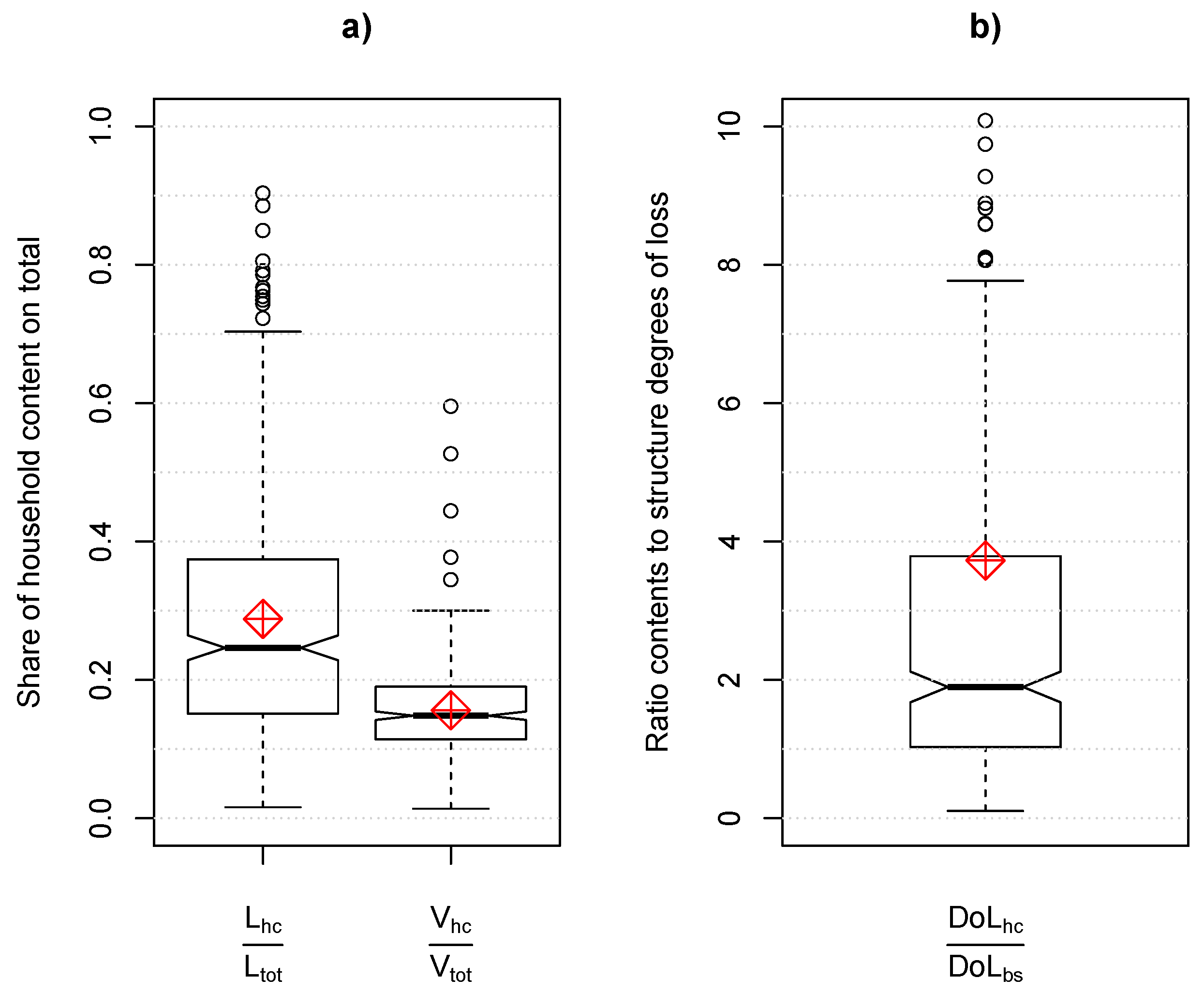
As we are interested in the role of content losses and vulnerability compared to structural losses, we calculate as a first overview the shares of content losses and insurance sums on total (structure + content) building losses and building values (see Figure 2). This will help us to make comparisons with other studies and reports of past events.
2.2. Regression Model
In this study, we used a linear regression [41,42] for the estimation of losses on household contents caused by flood events. The main objective of the regression analysis is to derive losses on household contents (as monetary [CHF] loss and as degree of loss [-]) from losses occurring on building structures at the same location and caused by the same event. Consequently, we use respectively the monetary loss and the degree of loss on household contents as the dependent variable and the corresponding type of loss on building structures as the only independent input to estimate the intercept and the slope parameter of the regression.
2.2.1. Data Transformation and Fitting
As indicated by Figure 1, the distributions of monetary losses and degrees of loss are even on the log scale both characterized by a right skew and therefore not normally distributed, nor do they follow a log-normal distribution (i.e., the logarithm of a variable is normally distributed). As normality of the involved variables themselves is not a prerequisite in classical linear regression analysis [43] (p. 92), this issue was not further examined. Instead we focus on the characteristics of the residuals produced by the linear model. This requires the consideration of heteroscedasticity, which is given when the variability of the response is not constant across the range of the explanatory variables. It can for example be adressed, visually with diagnostic plots or more formally by the Breusch-Pagan (BP) test [44]. Further, the assumption of normally distributed residuals has to be met as well [43,45] and will be tested by the Shapiro-Wilks (SW) test for normality [46]. We will also use diagnostic plots as visual aids for interpretations. Gaussian linear regression models with non-normally distributed residuals might lead to inaccurate confidence and prediction intervals and biased predictions. Not considering either of these assumptions will lead to an inaccurate estimation of the regression parameters.
For data initially not satisfying these properties, power transformations are common methods to achieve normality and an approximately constant residual variance in Gaussian linear regressions. Out of this family, the Box-Cox transformation, defined for as
where is the power parameter and denotes the transformed version of y, is a special case [47,48,49,50,51,52]. To return to the original scale of the data, the values can be back-transformed by using
The advantages of this transformation compared to other members of the power family are the systematic determination of the power parameter by maximum likelihood estimation [53] (p. 278) and the continuity at = 0 [52] (p. 67). Consider the linear regression model with a single covariate x given by
where y and x denote response and covariate respectively, and are the regression coefficients to be estimated and the error is assumed to be normally distributed with variance . Originally the Box-Cox transformation would be applied to the response variable y so that y in Equation (3) is replaced by , but an application to other non-negative quantities is of course also possible. Carroll and Ruppert [49] and Ruppert and Matteson [52] introduced the transform-both-sides (TBS) method, which consists in transforming the response y and the deterministic part of the regression equation with the same power parameter so that the model Equation (3) becomes
This approach was actually developped for cases where the response y is known to theoretically satisfy a given non-linear function of x and some unknown parameters , but where the residuals from the corresponding model on original scale would not satisfy normality and/or homoscedasticity. In our application of this model, we chose the linear structure because it does not seem too bad based on a scatterplot of the data and because we had no other a priori guess for the relation between y and x for the loss data. To nevertheless account for possible non-linearity between the two quantities, we also applied another model we termed pseudo-transform-both-sides (PTBS). It consists of the same linear regression structure applied to Box-Cox transformations of y and x, i.e.,
In a first step we used the same power parameter for both transformations as given here, but due to slightly sub-optimal model diagnostics especially for the absolute loss data, we also fitted the following extension of the PTBS model with two different power parameters for x and y (later referred to as PTBS.seplam):
For all three models, the complete parameter set can be estimated by maximum likelihood estimation, so that standard errors and confidence intervals for all parameters are easily obtained.
The Bonferroni Outlier Test was used to detect exceptional data points [45]. We also calculated Cook’s distance, leverage and defined large residuals. Once the regression parameters are estimated and all model assumptions verified, the edited regression has to be back-transformed to retrieve the original and interpretable unit, resulting for the PTBS model in:
The back-transformation being non-linear for the PTBS and PTBS.seplam models, the residuals are not any more normally distributed as they were in transformed form [53,54,55,56]. In addition, mean and median of the back-transformed distribution no longer coincide. When < 1, the power parameter for the back-transformation becomes > 1 which means that the normal distribution of the residuals on the transformed scale gets right-skewed on the original scale [57]. The right skew implies a discrepancy between the median and the mean of the back-transformed distribution such that the former systematically underestimates the latter. Taylor [55] derived an approximation for the conditional mean of the untransformed response variable y in terms of the model parameters , , , for the original Box-Cox model, where is linear in x, i.e., . Adopted to the PTBS model it reads
where the unknown residual value is set to zero. Replacing the parameters , , , in (8) by their maximum likelihood estimates yields an estimate for the mean of the original variable Y. The variance of can then be estimated by the delta method (e.g. Weisberg [58]) and confidence intervals (and prediction intervals) for can be based on the asymptotic normality of the maximum likelihood estimator.
2.2.2. Cross-Validation
To test the predictive accuracy of our models and their robustness in terms of variance and bias, a leave-one-out cross-validation was applied [59,60]. For each model type (PTBS, PTBS.seplam, TBS as well as relative or monetary loss), every single observation is predicted as either the median or the mean from the model fitted to the data set without observation . For the resulting sample of predictions, the aggregate prediction error is computed as the mean of the prediction errors for the individual observations . In addition we computed the standard deviations for each prediction error sample as a measure of the spread of the individual prediction errors. To compare the prediction quality and accuracy of the different models we considered four different error metrics for each case: bias [CHF], relative bias [%], absolute error [CHF] and relative absolute error [%] [61].
For comparisons in terms of accuracy, the results of both the monetary loss model and the model based on degrees of loss need to describe the same unit and scale. We use the unit [CHF] for evaluating the models. To do so, predicted degrees of loss on household contents are multiplied by the insurance sum of the content, provided by the insurance company.
2.2.3. Assessment of Transferability
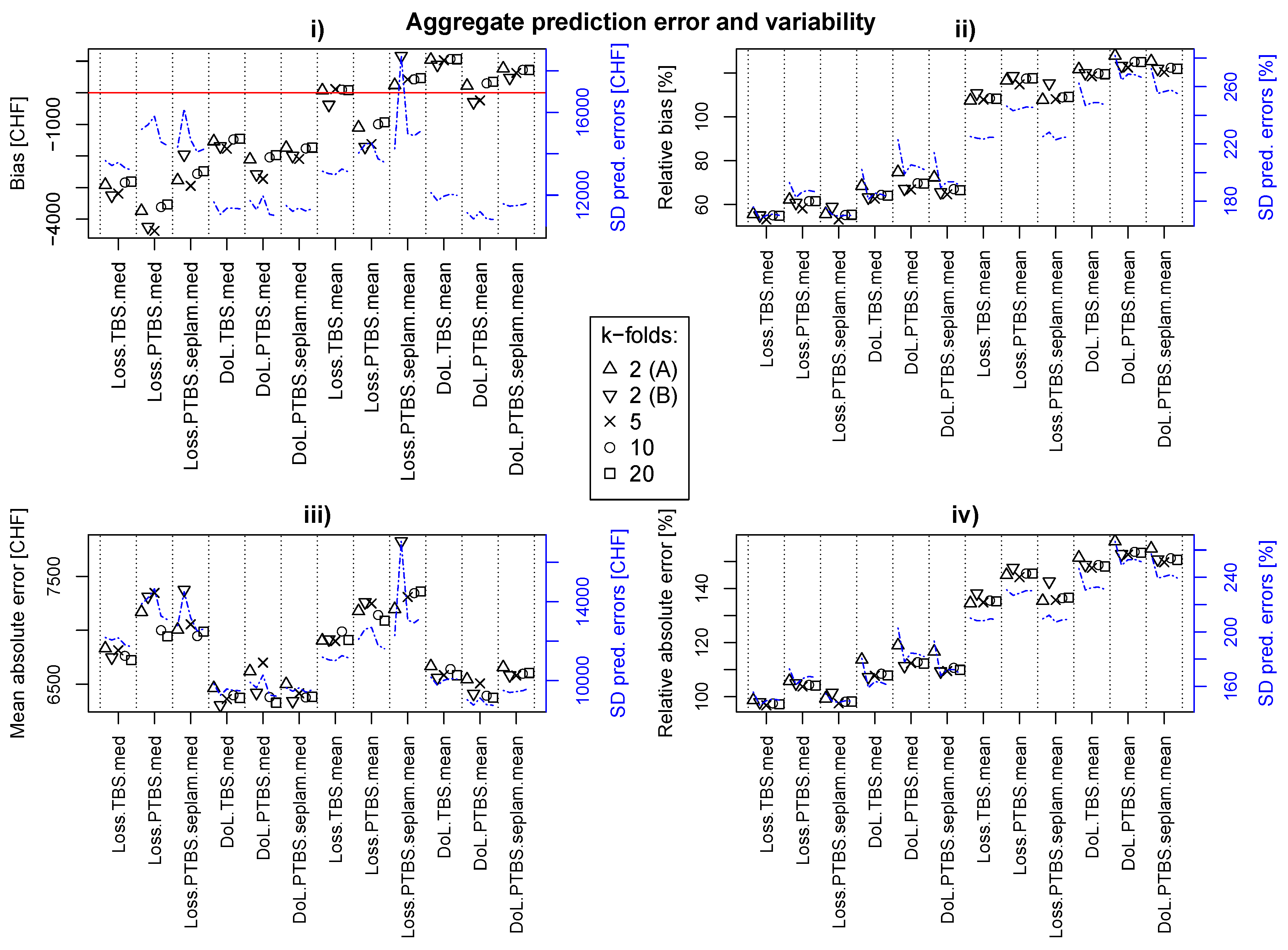
Based on Wenger and Olden [62], who suggest non-random cross-validation by splitting data into geographic regions, we analysed the performance of our models in terms of transferability. We applied the non-random cross-validation based on monetary losses to data from five out of seven available cantons. The cantons of Geneva and Appenzell Inner-Rhodes were neglected because only few claims were found with both structure and content loss. The transferability assessment for our models was tested for Obwalden (n = 110), Ticino (83), Uri (90), Schwyz (77) and Valais (19).To make sure that the unbalanced sample sizes of the cantons do not impact the results, we applied non-random K-fold cross-validation for several numbers of folds K between 2 and 20. In the last case, the fold sizes are similar to the “outlying” Valais sample size. We used the same error metrics for this analysis as for the leave-one-out cross-validation.
As a further assessment of transferability, we carried out an analysis of variance (anova) [58,63] on the transformed data, assuming fixed. More particularly, we tested whether a model with individual regression lines for each canton (differing either only in the intercept or in intercept and slope) fits the data better than the simpler model with a single line. Good transferability of the current simple model is then achieved if the more complex version with individual regression lines leads to no significantly improve fit.
3. Results
3.1. On the Role of Household Contents
The box plots of the shares of household content loss (left) and insurance sum (right) on total building loss and insurance sum are shown in Figure 2a. The mean share of content loss amounts to 0.29 (=29%), whereas the median is roughly 25%. With respect to the share on the total building value (mean: 0.16; median: 0.15), this is disproportionately high. Accordingly, the degree of loss of contents is generally higher than the degree of loss of building structure, as shown in Figure 2b. The interquartile range lies between 1.03 and 3.73 (median = 1.9, mean ≈ 3.7), which implies that in nearly three quarters of all losses, household content is more vulnerable than building structure.
3.2. Model Fitting
As mentioned in Section 2.2.1, we fitted different models to both types of loss data. Although the model fit is slightly advantageous for the TBS and the PTBS.seplam model, we define the PTBS model (regression function fitted after transformation by the same for both sides) as the best model, due to its better performance in terms of predictive power. Therefore, in the following two subsections, we will only present results for this specific model.
3.2.1. Data Transformation
The 95% confidence interval (CI) for obtained by profile maximum likelihood estimation indicates a range with plausible values for . For degrees of loss, the method proposes to use = 0.205, CI: as transformation parameter. Weisberg [50] recommends to use a rounded value for . Because none of the suggested values lies within the range of our CI, we select the exact estimate of . Indeed we do not consider , which would be covered by the CI, to be more easily interpretable in terms of the original variable y than .
For monetary loss, the best estimate and 95% CI of are 0.131 and , respectively. We use the exact value of for the same reasons as before.
3.2.2. Regression Model
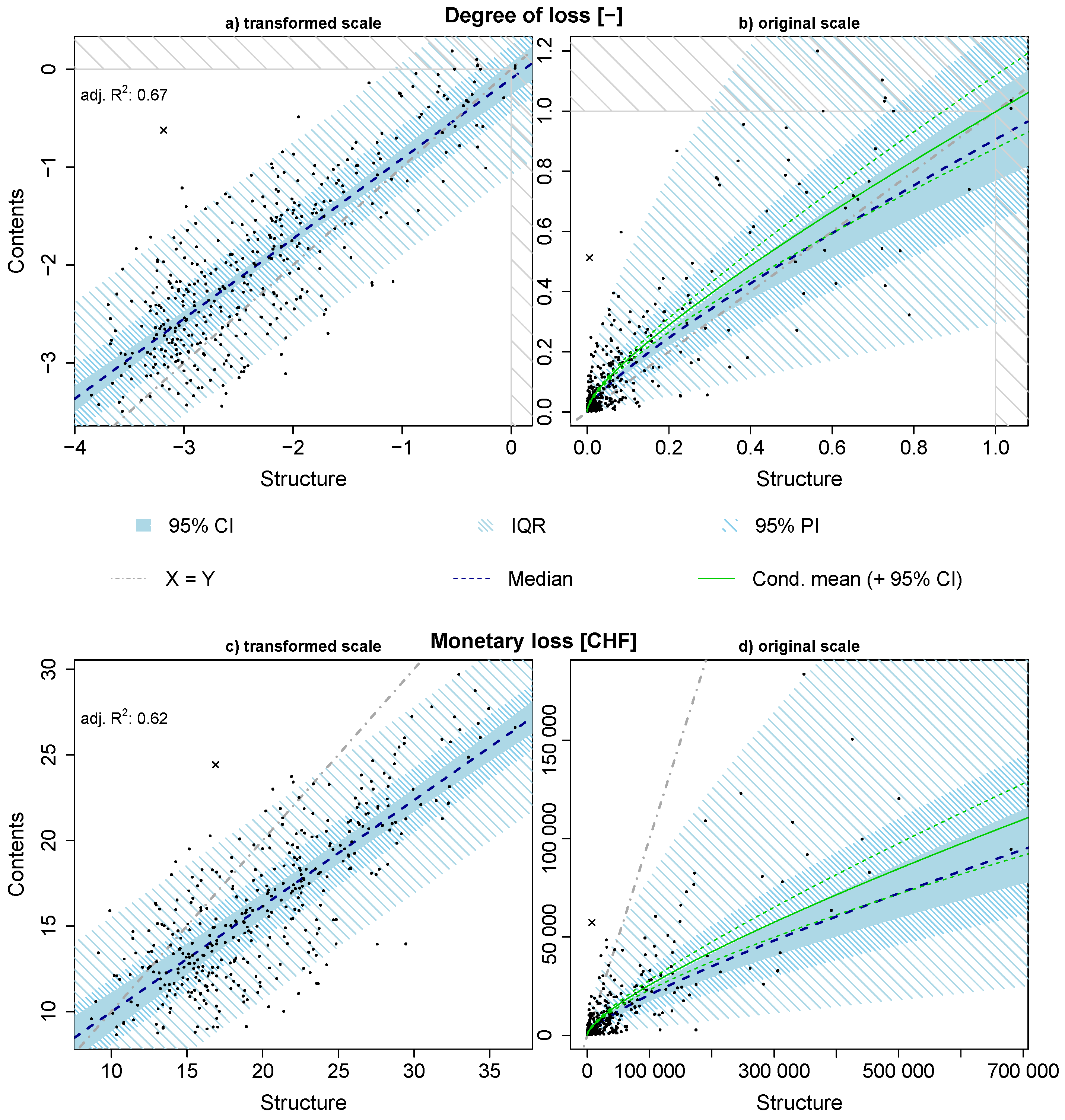
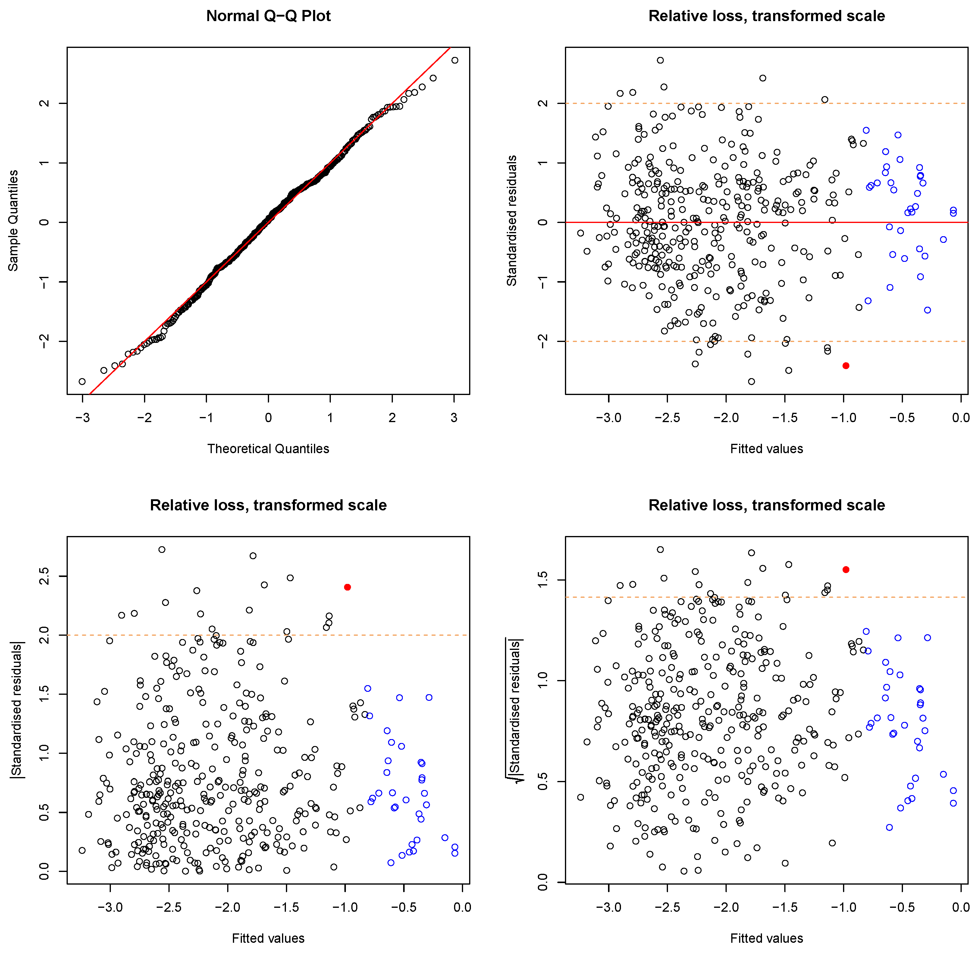
The result of the PTBS approach and the regression based on transformed degrees of loss can be examined in Figure 3a. Kendall’s (0.556) and Spearman’s (0.746) suggest to reject the null hypothesis of non-correlation of the degree of loss of building structure and household content. The F-statistic of the model indicates significant linearity and the adjusted R reaches 0.668. Here, the CI of the intercept parameter is (−0.255, 0.060) which indicates that the regression line goes roughly through the origin and the intercept parameter is not significant. A visual insight into the diagnostic plots for the model based on degrees of loss is given in Figure A1 in the Appendix. Based on the patternless scatter of the standardised residuals plotted against the fitted values (Figure A1, top right), the standardized residuals following a normal distribution (Figure A1, top left) and emphasized by the Shapiro-Wilks test (SW: p-value = 0.385), normality cannot be rejected. In addition, the Breusch-Pagan test indicates that the null hypothesis of the residuals being homoscedastic cannot be rejected either (BP: p-value = 0.742), which is also indicated by the scale-location plot (Figure A1, bottom right) not showing severe changes in variance. The monetary loss model also meets the requirements of a linear regression relatively reasonably. The model produces residuals which are not significantly different from a normal distribution (SW: p-value = 0.245) and not significantly heteroscedastic (BP: p-value = 0.221). Linearity is significant as well (adj. = 0.618, see Figure 3c), the diagnostic plots are shown in Figure A3. Note that there is a slight pattern in residuals plotted against the fitted values, indicating a minor lack of fit. An overview of all parameter estimates (, , and ) is given with Table A1, their confidence intervals (95%-CI) and statistical measures for the resulting models indicating the model quality (Shapiro-Wilks and Breusch-Pagan tests, Spearman’s , Kendall’s and the coefficient of determination (adj. )).
After substitution of the model parameters in Equations (7) and (8), respectively, the regression is not linear any more, because the back-transformation of the Box-Cox method leads to a non-linear function. Figure 3b,d show the final results of the model optimization process on the original scale. In Figure 3b, the concavity of the regression function points out that especially for objects where a low degree of loss was observed, the ratio of degree of loss of contents to the degree of loss of structure is generally higher than in cases, where high vulnerabilities were recorded. The major part of the household contents shows higher degrees of loss than the building structures.
The monetary loss model, which allows a direct estimation of loss on household contents based on the loss that occurred on building structure, shows that structure loss is in general considerably higher than the corresponding household content loss (see Figure 3d). Poor predictive power is found on higher magnitudes (building structure losses > ca. 320,000 CHF). Here, the model underestimates the content loss.
3.3. Cross-Validation
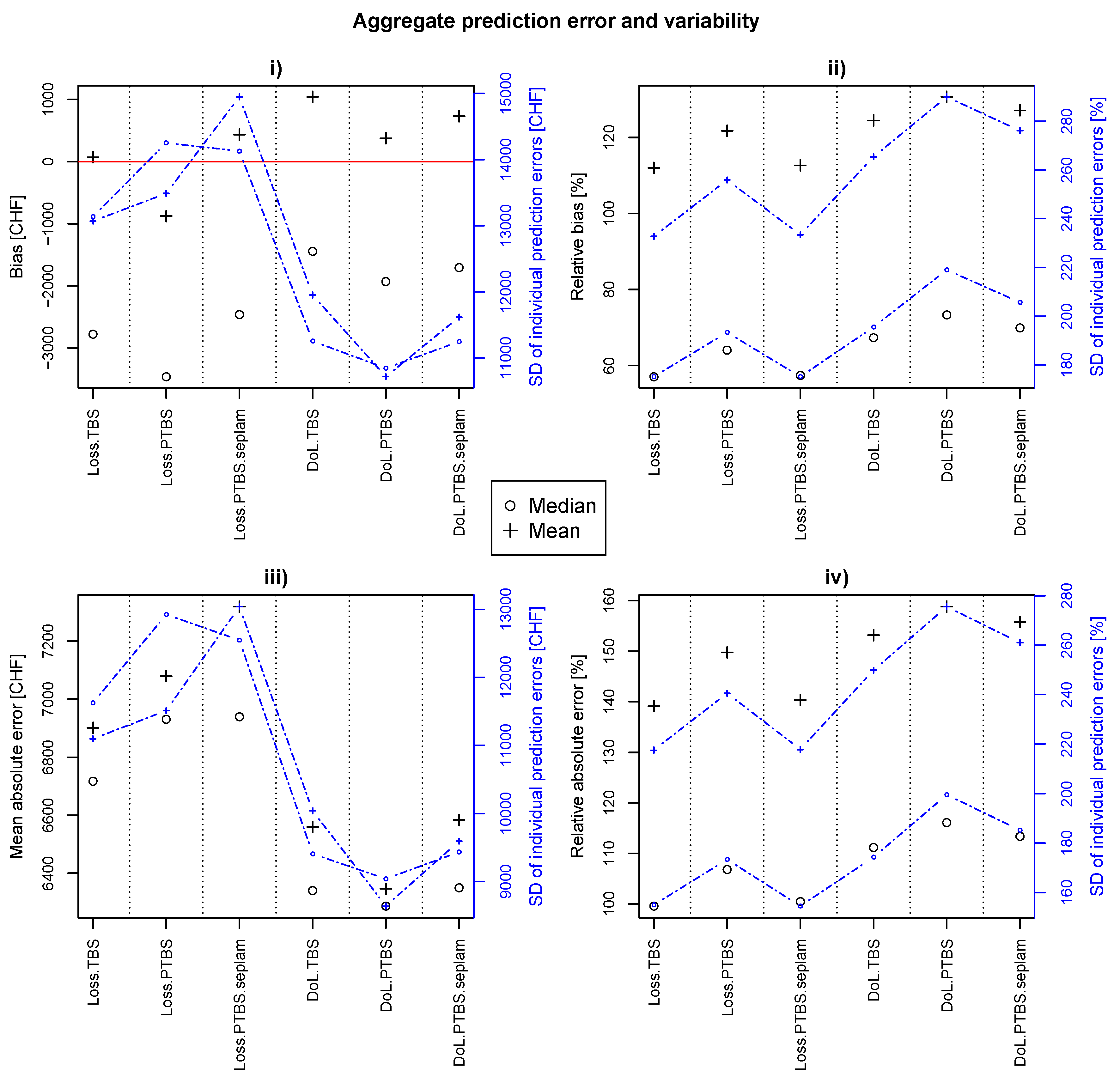
The metrics resulting from the leave-one-out cross-validation are presented in Figure 4: (i) bias; (ii) relative bias; (iii) mean absolute error and (iv) relative absolute error. Here, results for the alternative models (TBS and PTBS.seplam) are presented as well. The position of the black symbols indicates the aggregated prediction error of the cross-validation, the dots along the dashed blue line indicate the standard deviation of the individual prediction errors. To compare model accuracy in the same unit (CHF), the predicted degrees of loss (DoL) on household contents were multiplied by the insurance sum.
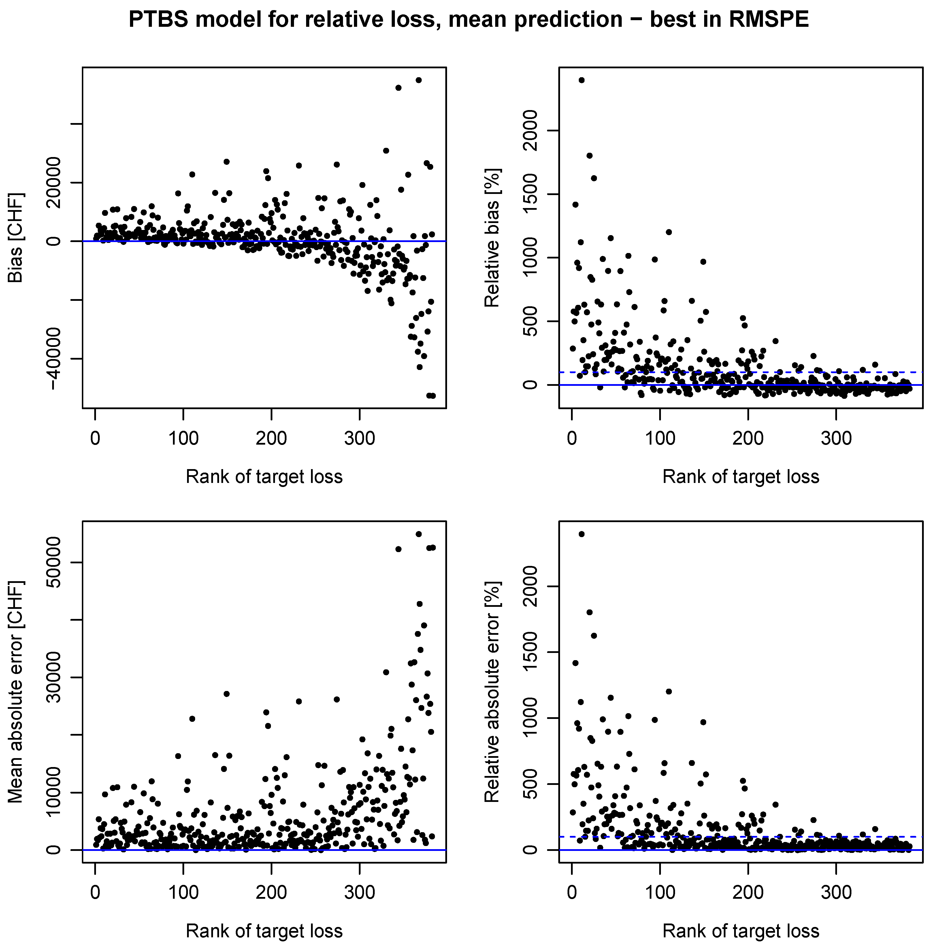
In terms of bias (Figure 4i), we first of all see that there is a clear improvement from median to mean estimation for both, the relative and absolute loss models. Second, we observe that the relative loss model with median estimation performs better, whereas there is no clear “overall” pattern for the mean estimates. Within the the groups (Loss.med, DoL.med, Loss.mean, DoL.mean), differences in performance are rather small. Apparently, the relative loss models show lower mean absolute prediction errors (Figure 4iii). Regarding this particular metric, we can say that estimations by median perform slightly better than by mean. Interestingly, the standard errors of the TBS and PTBS absolute loss models and for the PTBS relative model lower mean prediction, whereas the metric itself gets higher. Looking at the two relative metrics (Figure 4ii,iv), we see that they are very similar to each other. On one hand, we can observe that median prediction is in terms of these relative metrics more accurate and on the other hand that the TBS and PTBS.seplam model supply roughly the same quality-better than the PTBS model. Figure A5 also shows, that relative errors (Figure 4ii,iv) are mainly large for lower loss values, whereas large absolute errors (Figure 4i,iii) rather occur in estimations of high losses. This in turn is not surprising, as the loss is, relative to the loss magnitude, larger for smaller losses. Hence a prediction of a small loss more easily misses the target by a few orders of magnitudes, resulting in a relative prediction error of several hundred percent while its absolute prediction error in CHF is still rather small compared to the larger loss values in the data. On the other hand, a small percentage (relative error) of a large loss can correspond to a large amount of money (absolute error). We also tested the behaviour of the Box-Cox transformation in the re-sampling process and found that the estimation of is robust.
In this study, we focus on the estimation of monetary flood losses, so we prioritize absolute to relative accuracy of the models. In the following summary describing the major findings concerning the absolute and relative loss models, we just mention absolute bias and mean absolute error: (a) The accuracy of predicting monetary loss is higher when derived by the relative loss model instead of the monetary loss model; (b) The standard deviation in the error samples show that prediction variance is lower for the relative loss models which is accompanied by higher robustness; (c) Although median estimation is able to compete with the mean estimation in terms of mean absolute error, it has clear disadvantages concerning bias. In the end, the fact that the PTBS model shows highest robustness and the best predictive accuracy, we selected this model to focus on and finally present in this study. We will use this model for the relative and absolute loss model although for the latter, the TBS model showed slight, for us not meaningful competitive advantages. Please also note that prioritization of relative metrics would lead to a different, but also plausible choice.
3.4. Transferability
The analysis of variance for the relative loss model on transformed scale indicates a significant improvement in the overall fit for both PTBS models when separating the intercept according to cantons (likelihood ratio test at 5% level) while such a seperation is not significant for the TBS model. However, this is not the case for the slope, meaning that there is only a shift of the regression line (on transformed scale) along the vertical axis. The non-significance of the slope parameter implies that the relative increase of the vulnerability of household contents to an increase of the vulnerability of the building structure stays stable and is not significantly different across cantons.
In view of the apparently significant difference between the intercepts and thus the overall magnitudes of degrees of loss for cantons, one would want to detect which cantons (or groups of cantons) are most different from others. A first straightforward, but rather innocent approach would be to assess the significance of all differences between pairs of intercepts by performing a t-test at a given level for each of them. Yet we believe that properly answering this question involves so-called a posteriori comparisons Sokal and Rohlf [63] (Chapter 9), all the more that we had no a prioi guess on which cantons might exhibit the largest differences before looking at the data. Performing such comparisons falls into the large field of multiple testing or multiple comparisons, which roughly speaking means that to reach an overall uncertainty level of on several tests, the single sub-tests have to be carried out at much smaller significance levels than . This in turn means that less significances tend to be found. We applied most approaches to this problem described in Sokal and Rohlf [63], but they did not lead to coherent results. Moreover, the whole matter is complicated because the sample sizes of the different cantons are not equal and their variances (still on transformed scale) seem to be significantly different, whereas many multiple comparison methods do strictly speaking not apply without the assumption of sample sizes and constant variances for all groups. We therefore do not present any further “results” of this analysis here because they are in our opinion not sufficiently well-founded, but refer to the discussion in Section 4. Interestingly, the difference in the intercept is only observed for the relative and not for the absolute loss model, although both models rely on the same loss data set.
As our model with only one covariate is rather simple, the tendency for over-fitting as described by Wenger and Olden [62] is expected to be rather small. This is indeed confirmed by the results of the non-random cross-validation, which are very similar to those found with the leave-one-out cross-validation (see Figure A6). Here, the models with high prediction accuracy thus also show the best performance in terms of transferability.
4. Discussion
With approximately 29%, the mean share of content loss on the total loss of residential buildings (structure + household contents) is similar to those found by Thieken et al. [31] (28%) or FOWG [32] (36.5%). Although we found comparable results in terms of the share of content loss on the total building loss, the data (monetary losses and degrees of loss) in our study were distributed over a lower range of magnitudes than in the analysis of Thieken et al. [31] for the Elbe and Danube floods. As mentioned in Section 3.1, regions with lower loss magnitudes showed in general a higher share of content loss on total building losses. This is emphasised by the facts, that the share on the loss is disproportionately high compared to the share of the content value to the total building value and, as seen by the linear regression in Figure 3a,b, the content loss to structure loss ratio is high especially for lower magnitudes. Therefore, as the loss magnitudes given by Thieken et al. [31] are higher, the mean share of content loss on the total building loss is rather high based on the findings in this study. Possible reasons are manifold and should be further studied, for instance different vulnerabilities of the buildings due to their type, differences of the hazard process (suspension load, dynamic or static inundation, caused by flooding of rivers in inclined topographies and inundation by a raising lake level, respectively, time of exposure, forecast accuracy of the event etc.). Preparedness may matter in this case as well: As insuring structure and contents in the regions analysed here is voluntary, contractors of insurance companies might be in general more sensitive to flood risks than others, and thus might be more resilient to such events. To our knowledge, this was not the case in the studies of Thieken et al. [31]. Another explanation for the differences in Thieken et al. [31] and FOWG [32] might be that in their studies content and structure losses need not necessarily be linked to each other. So the structure and content data sets do not have the same origin and thus, their results are not directly comparable with those of this study.
Uncertainty exists because information on the total number of flood-affected buildings and household contents is missing. This implies that we cannot make comparisons of loss frequency for building structure and household contents, respectively. Thus, we leave open the question of how probable a household content loss occurs when building structure is affected (and vice versa). Moreover we did not consider either that one building might consist of more than one household (in this study up to three). Depending on how the building is arranged, for instance with one apartment on the ground floor and two on upper floors (or vice versa), where water levels rarely rise to, content losses might get less (or more) relevant in the total building loss. Residents from upper floors storing contents on the underground floor might play a role in this context as well. We neglected those points and focused on examples where only both in combination, building structure and household content losses, occurred. In terms of total loss prediction, we point out that this is a crucial issue and that those points can make the difference between successful and failed predictions.
Furthermore, there are some methodical restrictions that have to be addressed. As we filtered the data by insurance sum, monetary loss and product type, the results are just valid for buildings with an insurance sum higher than CHF 100,000, losses above CHF 100 and with a residential purpose with maximum three apartments. Hence, attention has to be paid when comparing our results or applying the presented models to other data.
By applying the transform-both-sides (TBS) methodology after Carroll and Ruppert [49] to our data, we found a way to meet the assumptions of Gaussian linear regression models concerning homoscedasticity and normality in the distribution of the residuals. There is one minor disadvantage: Due to the challenges of the back-transformation to make inferences in the original scale, a correction factor has to be calculated to derive the estimated mean. This makes the equation more laborious than other approaches, but reproducibility is still given. Alternatively to the proposed method of our study to find a mean estimation, one could also try to fit a generalized linear model. In addition, a quantile regression approach (see Davino et al. [64]) could be potentially useful. So far, in vulnerability and flood loss prediction, the presented method was never used before and the benefits are shown by its reproducibility, the possibility for a systematic application in other study areas and considering the prediction uncertainties. Our models indicate a high robustness of estimating , ensuring normality and homoscedasticity for the residuals resulting from the subsequent linear regressions.
One objective of this study was to deduce whether the prediction of household content losses performs better by a loss model based on degrees of loss, looking at the relation of loss ratio (loss/insurance sum) occurring on content and structure or by a direct loss model connecting monetary loss on household content with the loss on building structure. For the model based on degrees of loss, we found one basic similarity as already presented by Jonkman et al. [27]: for the lower intensity level on structure, with the increase of the degree of loss of structure, the degree of loss on household contents comparatively increases following a concave function. This leads to a larger ratio of degrees of loss of contents to degrees of loss of structure at low levels. This emphasises the findings mentioned above, that especially for losses with low magnitudes, household contents are more vulnerable to floods than building structure and here, the role of losses on household contents might be essential.
As a consequence of the model characteristics mentioned and as a punctuating element of this statement, the regression of the monetary loss model shows a concave characteristic as well. This implies that the ratio of the monetary household content losses relative to the building structure losses is higher in low magnitudes compared to high ones. Although the model statistically meets all demanded requirements (normality, homoscedasticity, robustness and, to some restrictions we discuss afterwards, also transferability), we see in Figure 3 that for the highest structure losses, the predicted content loss is underrated systematically. This could also be the reason that leads to the (slight) tendency for negative bias and underestimation of the total loss we found in (non-)random cross-validation. As these high values mainly occurred in the canton of Obwalden, we cannot clearly say if this issue originates in methodical inadequacies or just local conditions. With respect to the analyses done by Carisi et al. [36], we didn’t only select our model by the best performance concerning error metrics, but also in compliance with statistical requirements. As we also did not need to predefine the type of transformation, the method used in this study has advantages in it’s flexibility and strong adaptiveness.
Comparing the quality of the two PTBS models, the accuracy of the model based on degrees of loss is advantageous as shown by the model fit, the absolute bias and the mean absolute error. This includes tests for normality and homoscedasticity (Table A1 and Figure A1 and Figure A3), robustness (Figure 4) and transferability (Figure A6, absolute errors). Concerning the analysis of variance, several uncertainties remain. First of all, the application for the TBS approach turned out to be very complex and there is still potential for improvement. We can clearly say that for the relative loss model based on degrees of loss, a difference in the intercept parameter exists, but we cannot clearly define the source that leads to the differences. With a variety of correction methods for the anova, we found that only differences between a combination of three groups are significant, but not between any pair of cantons. We mention that there are also uncertainties in the proceeding and methodical correct utilization of the methods in detecting the relevant differences, not leas because of unequal group sizes and variances; see also Section 3.4. As mentioned, there is no improvement by distinguishing the origin of the losses in the absolute loss model. Here, it is plausible that the higher variance and the lower model fit prevents the intercept parameter from being significantly different. To conclude, although uncertainties exist, we still would interpret the relative loss model as transferable, justified in accordance with the intercept parameter statistically not being significant in model fitting, but we also point out, that further analysis and improvements are required. In particular, we acknowledge that a more in-depth statistical analysis of these uncertain aspects is not infeasible and would most likely also lead to improved answers, but simply was beyond the scope of this study.
The random cross-validation underlines the relative loss model being more robust than the monetary model, by returning lower error standard deviation and improved accuracy concerning the absolute error types. In addition, we expect advantages of the relative loss model concerning reliability, being independent of the value of an object. This means in detail that for the monetary loss model a constant ratio of content and structure values is assumed, whereas the relative loss model is independent of the variety of possible value-combinations, e.g., valuable contents being located in low-priced buildings etc. The dependence of the monetary loss on the value is also shown by Thieken et al. [31], where variables describing value and size are highly relevant for monetary losses, whereas for the degree of loss this effect is remarkably reduced by putting the monetary loss value in relation to the monetary value of the object. We suppose that this could be the reason why variance and the model fit in the relative loss model are more accurate. We point out that with degree of loss and monetary loss of structure as only input variables, the relative and monetary models are able to explain 67% and 62% of the variance in degrees of loss and monetary loss of contents, respectively. We explain these high values with two out of three main components (flood variables and preparedness) found by Thieken et al. [31] being neutralized through our approach: As we analysed contents and structure being part of the same building, the interacting flood variables are the same and thus neglectable. The same is valid for preparedness: We linked contracts of contents and structure referring to the same person with obviously the same preparedness. In conclusion, indirect models for household contents as presented here are supposed to be more transferable than vulnerability curves for household contents. The models presented here might be linked with existing, often locally valid vulnerability curves for building structure loss. Those functions and models created by fitting flow parameters (and structural characteristics) to empirical loss data implicitly contain information about the susceptibility of building structure and therefore also to household contents (e.g., resistant structures might prevent contents from strong exposition). Compared to the classical model, the indirect model type presented here and in Carisi et al. [36] can also be used to complete loss estimations when higher accessible loss data on structure is known, for instance to provide total loss estimations during flood events. As the models are depending on either vulnerability functions for building structure generating the degree of loss (or monetary loss) or on the loss data of building structure themselves, the limitations of these dependencies are as well transferred to models presented. In addition, the restrictions mentioned have to be considered as well.
5. Conclusions
Based on reliable data and established literature, we showed that household content loss is a relevant factor in the estimation of flood losses and should be considered in future loss predictions or flood risk assessments. In relation to the average total loss of a building including content and structure loss, losses of household content contributes from 21% to 32% based on our data, whereas contributions of up to 36% are found in the literature. The results indicate that especially when low degrees of loss or monetary losses are caused by floods, the vulnerability of contents is clearly higher than the vulnerability of the corresponding building structure. Thus, assuming that generally high flood intensities lead to high losses, it has to be considered that the share of household contents on the total building loss is decreasing relatively in regions with comparatively high losses or degrees of loss.
We present two models, deduced from loss claims on residential buildings with maximum three apartments, which allow to predict the degree of loss or the monetary loss for household contents based only on corresponding losses on the building structure. Moreover, we tested and compared the models in terms of robustness, transferability and predictive power. Both models generate appropriate results with a comparative advantage of the relative over the monetary loss model. They meet the statistical requirements of normally distributed residuals with constant variance which is the basis for a robust model. As shown by random cross-validation, the absolute bias and standard deviation is generally low for both, but lower for the relative loss model. As well, the relative loss model is favourable being more transferable to new regions, as assessed by a non-random cross-validation. As important as that, flow parameters, preparedness and building characteristics-the most relevant parameters to generate direct vulnerability curves - can be neglected here because contents and structure are not only located at the same position, but also owned by the same person. The functions created here are supposed to be linked with locally validated vulnerability curves for building structures or structure loss data to complete total loss estimations. Nevertheless, attention should be paid when applying the functions in regions where the major part of degrees of loss or monetary losses is expected to scatter around the upper or lower range of our data set or just a very small number of data is available. In this case, we presented a method that quantifies uncertainties and supports the interpretation of the model accuracy.
The Box-Cox method is characterised by not insisting on a certain transformation. Instead, it takes into account a multiple set of power transformations (including the log-transformation) to reach normality and homoscedasticity of the residuals and suggests an appropriate -parameter based on the quantitative and reproducible maximum likelihood method. By applying tests to the residual distribution, we showed that this transformation method works well for general right-skewed loss data, and meets model assumptions of a Gaussian linear regression. For both, the degree of loss and monetary loss model, as the original data are strongly heteroscedastic, the uncertainties are rising with increasing values of exposed assets and losses. We recommend to consider data transformation, as it is providing a statistically correct estimation of the regression parameters and uncertainties.
Author Contributions
Conceptualization, M.M. and A.Z.; Methodology, M.M. and L.F.; Validation and Formal Analysis, L.F. and M.M.; Investigation, M.M., L.F. and A.Z.; Data Curation, M.M.; Writing—Original Draft Preparation, M.M.; Writing—Review & Editing, all; Visualization, M.M., L.F.; Supervision, A.Z., M.K., R.W.
Funding
This research was funded by the Mobiliar Lab for Natural Risks.
Acknowledgments
The authors thank Swiss Mobiliar Insurance Company for providing the data and especially Luzius Thomi and Rouven Sturny for advice on the interpretation of the data.
Conflicts of Interest
The founding sponsors had no role in the design of the study; in the collection, analyses, or interpretation of data; in the writing of the manuscript, and in the decision to publish the results.
Abbreviations
The following abbreviations are used in this manuscript:
| BP | Breusch-Pagan (test) |
| CI | Confidence Interval |
| DoL | Degree of Loss |
| FOEN | Federal Office of Environment |
| FOWG | Federal Office of Water and Geology |
| PSL | Pound Sterling Live |
| PTBS | Pseudo-Transform-Both-Sides |
| PTBS.seplam | Pseudo-Transform-Both-Sides with separate transformation parameters for x and y |
| SW | Shapiro-Wilks (test) |
| TBS | Transform-Both-Sides |
Appendix A
Appendix A.1
Figure A1.
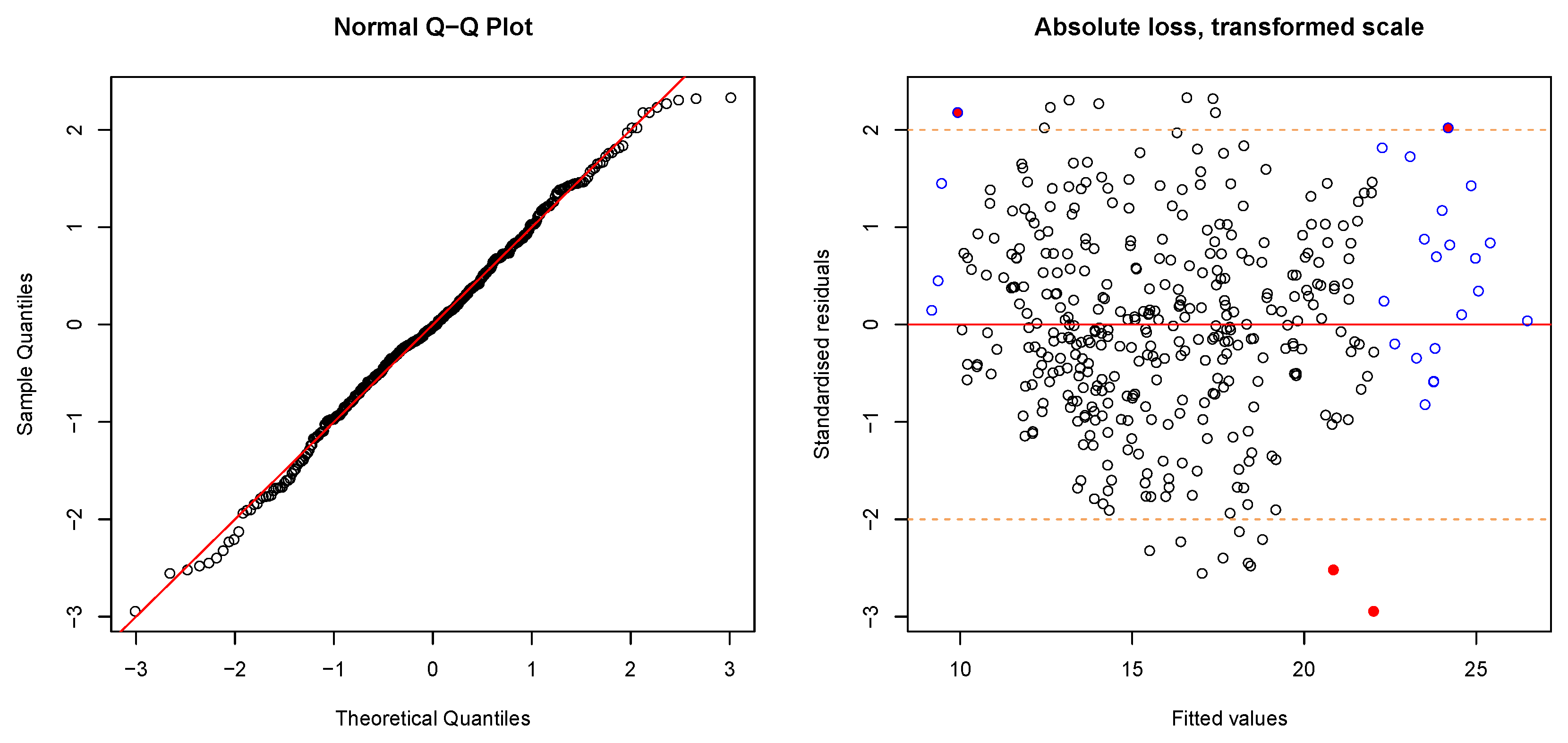
Diagnostic plots for the residuals (transformed degrees of loss) shown by Figure 3a. (Top left) Normal-Q-Q-plot, points along diagonal line don’t reject normality (SW: normality with a p-value = 0.385). All other figures show the fitted values on X-axis against the standardised residuals on the Y-axis as normal (top right), absolute (bottom left) and the square root (bottom right) of the absolute values. Blue borders indicate high leverage points, red filled circles indicate high values for Cook’s distance and the orange dashed lines indicate the borders to the definition of large residuals. Heteroscedasticity is not evident. One outlier (Bonferroni outlier test) is not shown in the plot.
Figure A1.
Diagnostic plots for the residuals (transformed degrees of loss) shown by Figure 3a. (Top left) Normal-Q-Q-plot, points along diagonal line don’t reject normality (SW: normality with a p-value = 0.385). All other figures show the fitted values on X-axis against the standardised residuals on the Y-axis as normal (top right), absolute (bottom left) and the square root (bottom right) of the absolute values. Blue borders indicate high leverage points, red filled circles indicate high values for Cook’s distance and the orange dashed lines indicate the borders to the definition of large residuals. Heteroscedasticity is not evident. One outlier (Bonferroni outlier test) is not shown in the plot.

Appendix A.2
Figure A2.
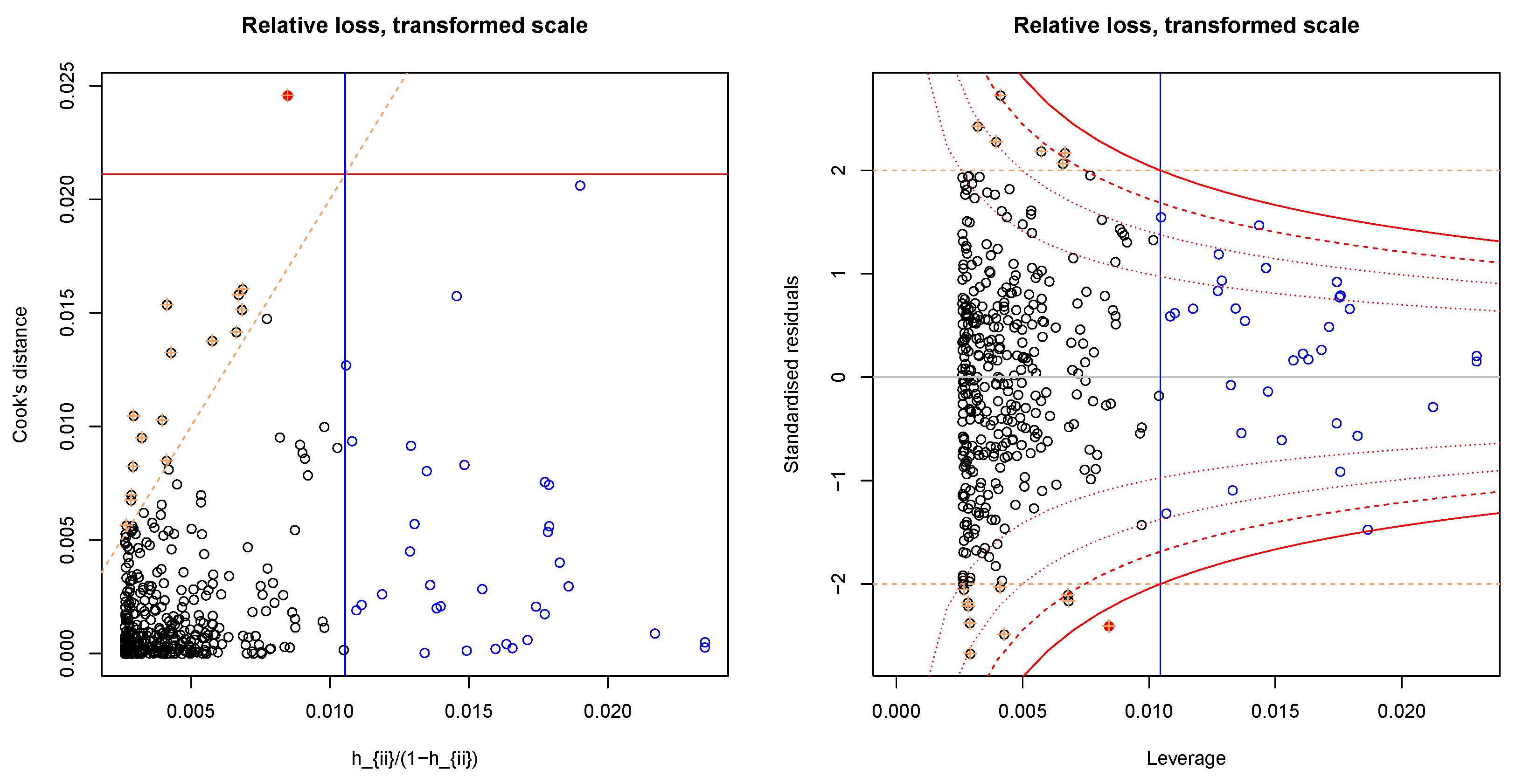
Leverage (X-axis) vs Cook’s distance (left) and standardised residuals (right) for the relative loss model on the vertical axis. Blue borders indicate high leverage points, red filled circles indicate high values for Cook’s distance and the orange dashed lines indicate the borders to the definition of large residuals. One outlier (Bonferroni outlier test) is not shown in the plot.
Figure A2.
Leverage (X-axis) vs Cook’s distance (left) and standardised residuals (right) for the relative loss model on the vertical axis. Blue borders indicate high leverage points, red filled circles indicate high values for Cook’s distance and the orange dashed lines indicate the borders to the definition of large residuals. One outlier (Bonferroni outlier test) is not shown in the plot.

Appendix B
Appendix B.1
Figure A3.
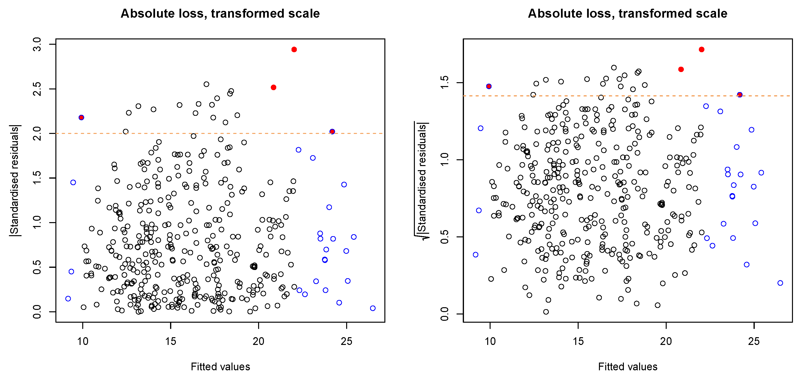
Diagnostic plots for the regression showed in Figure 3c. (Top left) Normal-Q-Q-plot, points along diagonal line don’t reject normality (SW: normality with a p-value = 0.245). All other figures show the fitted values on X-axis against the standardised residuals on the Y-axis as normal (top right), absolute (bottom left) and the square root (bottom right) of the absolute numbers. Blue borders indicate high leverage points, red filled circles indicate high values for Cook’s distance and the orange dashed lines indicate the borders to the definition of large residuals. Heteroscedasticity is not evident. One outlier (Bonferroni outlier test) is not shown in the plot.
Figure A3.
Diagnostic plots for the regression showed in Figure 3c. (Top left) Normal-Q-Q-plot, points along diagonal line don’t reject normality (SW: normality with a p-value = 0.245). All other figures show the fitted values on X-axis against the standardised residuals on the Y-axis as normal (top right), absolute (bottom left) and the square root (bottom right) of the absolute numbers. Blue borders indicate high leverage points, red filled circles indicate high values for Cook’s distance and the orange dashed lines indicate the borders to the definition of large residuals. Heteroscedasticity is not evident. One outlier (Bonferroni outlier test) is not shown in the plot.


Appendix B.2
Figure A4.
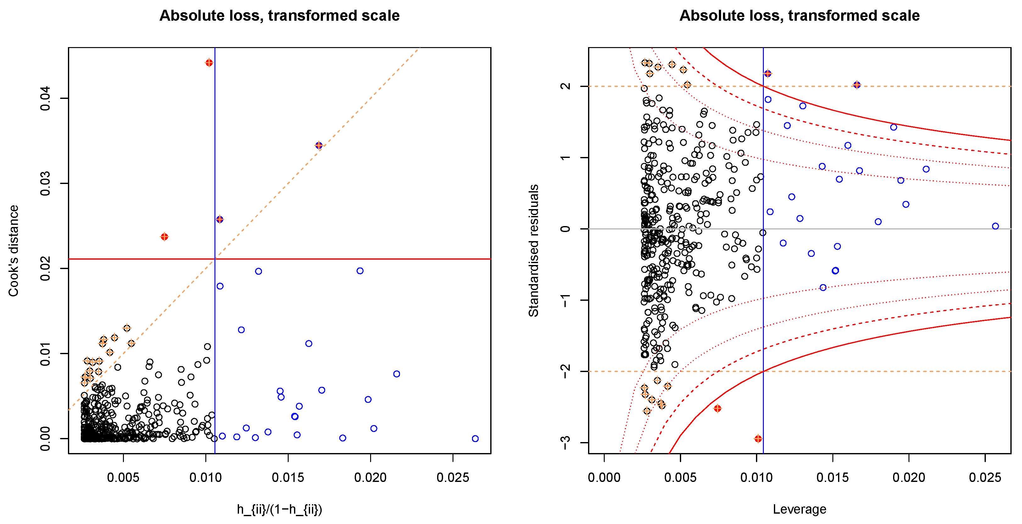
Leverage (X-axis) vs Cook’s distance (left) and standardised residuals (right) of the relative loss model on the vertical axis. Blue borders indicate high leverage points, red filled circles indicate high values for Cook’s distance and the orange dashed lines indicate the borders to the definition of large residuals. The outlier found for the relative loss model (Bonferroni outlier test) is not shown in the plot and was not used during the model fitting procedure.
Figure A4.
Leverage (X-axis) vs Cook’s distance (left) and standardised residuals (right) of the relative loss model on the vertical axis. Blue borders indicate high leverage points, red filled circles indicate high values for Cook’s distance and the orange dashed lines indicate the borders to the definition of large residuals. The outlier found for the relative loss model (Bonferroni outlier test) is not shown in the plot and was not used during the model fitting procedure.

Appendix C
Figure A5.
Dependence of single errors on ranking. Absolute errors show high variability in higher ranks of target loss (original scale), whereas relative errors are more variable in lower ranks.
Figure A5.
Dependence of single errors on ranking. Absolute errors show high variability in higher ranks of target loss (original scale), whereas relative errors are more variable in lower ranks.

Appendix D
Figure A6.
Non-random cross-validation. K-fold = 2, (A): Obwalden + Ticino vs. Schwyz + Valais + Uri; (B): Obwalden + Schwyz vs. Ticino + Valais + Uri. K-fold = 5: One group per canton. K-Fold = 10/20: Split Obwalden, Ticino, Schwyz and Uri into multiple groups such that all groups have approximately the same size.

Appendix D.1

Table A1.
Overview of the statistical evaluation and parameters of the two selected models. The estimates of , , and can be substituted in Equation (7) or (8) to predict the median or mean of y, respectively. * 95%-confidence interval
| Relative Loss Model | Monetary Loss Model | |
|---|---|---|
| Spearman’s | 0.746 | 0.720 |
| Kendall’s | 0.556 | 0.527 |
| Maximum Likelihood Estimate | 0.205 | 0.131 |
| CI * | (0.144, 0.265) | (0.068, 0.193) |
| 0.495 | 2.745 | |
| −0.098 | 3.798 | |
| CI * | (−0.255, 0.060) | (2.179, 5.416) |
| 0.817 | 0.618 | |
| CI * | (0.750, 0.884) | (0.560, 0.676) |
| adjusted R | 0.668 | 0.618 |
| Shapiro-Wilks p-value | 0.385 | 0.245 |
| Breusch-Pagan p-value | 0.742 | 0.221 |
References
- United Nations International Strategy for Disaster Reduction (UNISDR). Global Assessment Report on Disaster Risk Reduction (GAR) 2015: Making Development Sustainable: The Future of Disaster Risk Management; United Nations: New York, NY, USA, 2015. [Google Scholar]
- Intergovernmental Panel on Climate Change (IPCC). Managing the Risks of Extreme Events and Disasters to Advance Climate Change Adaptation: Special Report of Working Groups I and II of The Intergovernmental Panel on Climate Change; Cambridge University Press: Cambridge, UK, 2012. [Google Scholar]
- Ward, P.J.; Jongman, B.; Weiland, F.S.; Bouwman, A.; van Beek, R.; Bierkens, M.F.P.; Ligtvoet, W.; Winsemius, H.C. Assessing flood risk at the global scale: Model setup, results, and sensitivity. Environ. Res. Lett. 2013, 8, 044019. [Google Scholar] [CrossRef] [Green Version]
- Sampson, C.C.; Smith, A.M.; Bates, P.D.; Neal, J.C.; Alfieri, L.; Freer, J.E. A high-resolution global flood hazard model. Water Resour. Res. 2015, 51, 7358–7381. [Google Scholar] [CrossRef] [PubMed] [Green Version]
- Alfieri, L.; Cohen, S.; Galantowicz, J.; Schumann, G.J.P.; Trigg, M.A.; Zsoter, E.; Prudhomme, C.; Kruczkiewicz, A.; Coughlan de Perez, E.; Flamig, Z.; et al. A global network for operational flood risk reduction. Environ. Sci. Policy 2018, 84, 149–158. [Google Scholar] [CrossRef]
- Hirabayashi, Y.; Mahendran, R.; Koirala, S.; Konoshima, L.; Yamazaki, D.; Watanabe, S.; Kim, H.; Kanae, S. Global flood risk under climate change. Nat. Clim. Chang. 2013, 3, 816–821. [Google Scholar] [CrossRef]
- Ward, P.J.; Jongman, B.; Aerts Jeroen, C.J.H.; Bates, P.D.; Botzen, W.J.W.; Diaz Loaiza, A.; Hallegatte, S.; Kind, J.M.; Kwadijk, J.; Scussolini, P.; et al. A global framework for future costs and benefits of river-flood protection in urban areas. Nat. Clim. Chang. 2017, 7, 642. [Google Scholar] [CrossRef]
- Badoux, A.; Andres, N.; Techel, F.; Hegg, C. Natural hazard fatalities in Switzerland from 1946 to 2015. Nat. Hazards Earth Syst. Sci. 2016, 16, 2747–2768. [Google Scholar] [CrossRef]
- Swiss Re. Floods in Switzerland—An Underestimated Risk; Swiss Re: Zürich, Switzerland, 2012. [Google Scholar]
- Andres, N.; Badoux, A. Unwetterschäden in der Schweiz im Jahr 2016: Rutschungen, Murgänge, Hochwasser und Sturzereignisse. Wasser Energ. Luft 2017, 109, 97–104. [Google Scholar]
- Staffler, H.; Pollinger, R.; Zischg, A.; Mani, P. Spatial variability and potential impacts of climate change on flood and debris flow hazard zone mapping and implications for risk management. Nat. Hazards Earth Syst. Sci. 2008, 8, 539–558. [Google Scholar] [CrossRef] [Green Version]
- Ernst, J.; Dewals, B.J.; Detrembleur, S.; Archambeau, P.; Erpicum, S.; Pirotton, M. Micro-scale flood risk analysis based on detailed 2D hydraulic modelling and high resolution geographic data. Nat. Hazards 2010, 55, 181–209. [Google Scholar] [CrossRef] [Green Version]
- Zischg, A.; Schober, S.; Sereinig, N.; Rauter, M.; Seymann, C.; Goldschmidt, F.; Bäk, R.; Schleicher, E. Monitoring the temporal development of natural hazard risks as a basis indicator for climate change adaptation. Nat. Hazards 2013, 67, 1045–1058. [Google Scholar] [CrossRef]
- Fuchs, S.; Keiler, M.; Zischg, A. A spatiotemporal multi-hazard exposure assessment based on property data. Nat. Hazards Earth Syst. Sci. 2015, 15, 2127–2142. [Google Scholar] [CrossRef] [Green Version]
- Fuchs, S.; Röthlisberger, V.; Thaler, T.; Zischg, A.; Keiler, M. Natural Hazard Management from a Coevolutionary Perspective: Exposure and Policy Response in the European Alps. Ann. Am. Assoc. Geogr. 2016, 1–11. [Google Scholar] [CrossRef] [PubMed]
- Zischg, A.P.; Mosimann, M.; Bernet, D.B.; Röthlisberger, V. Validation of 2D flood models with insurance claims. J. Hydrol. 2018, 557, 350–361. [Google Scholar] [CrossRef]
- Papathoma-Köhle, M.; Kappes, M.; Keiler, M.; Glade, T. Physical vulnerability assessment for alpine hazards: State of the art and future needs. Nat. Hazards 2011, 58, 645–680. [Google Scholar] [CrossRef]
- Fuchs, S.; Frazier, T.; Siebeneck, L. Physical Vulnerability. In Vulnerability and Resilience to Natural Hazards; Fuchs, S., Thaler, T., Eds.; Cambridge University Press: Cambridge, UK, 2018; pp. 32–52. [Google Scholar]
- Fuchs, S.; Birkmann, J.; Glade, T. Vulnerability assessment in natural hazard and risk analysis: Current approaches and future challenges. Nat. Hazards 2012, 64, 1969–1975. [Google Scholar] [CrossRef]
- Papathoma-Köhle, M. Vulnerability curves vs. vulnerability indicators: Application of an indicator-based methodology for debris-flow hazards. Nat. Hazards Earth Syst. Sci. 2016, 16, 1771–1790. [Google Scholar] [CrossRef]
- Akbas, S.; Blahut, J.; Sterlacchini, S. Critical Assessment of Existing Physical Vulnerability Estimation Approaches for Debris Flows. In Proceedings of the Landslide Processes: From Geomorphologic Mapping to Dynamic Modeling, Strasbourg, France, 6–7 February 2009; Volume 67. [Google Scholar]
- United Nations Disaster Relief Organization (UNDRO). Natural Disasters and Vulnerability Analysis; Office of The United Nations Disaster Relief Co-Ordinator: Geneva, Switzerland, 1980. [Google Scholar]
- Totschnig, R.; Sedlacek, W.; Fuchs, S. A quantitative vulnerability function for fluvial sediment transport. Nat. Hazards 2011, 58, 681–703. [Google Scholar] [CrossRef]
- Papathoma-Köhle, M.; Zischg, A.; Fuchs, S.; Glade, T.; Keiler, M. Loss estimation for landslides in mountain areas—An integrated toolbox for vulnerability assessment and damage documentation. Environ. Modell. Softw. 2015, 63, 156–169. [Google Scholar] [CrossRef]
- Hydrotec. Hochwasser-Aktionsplan Angerbach. In Teil I: Berichte Und Anlagen; Studie im Auftrag desStUA Düsseldorf; Hydrotec Ingenieurgesellschaft für Wasser und Umwelt mbH: Aachen, Germany, 2001. [Google Scholar]
- Dutta, D.; Herath, S.; Musiake, K. A mathematical model for flood loss estimation. J. Hydrol. 2003, 277, 24–49. [Google Scholar] [CrossRef]
- Jonkman, S.N.; Bočkarjova, M.; Kok, M.; Bernardini, P. Integrated hydrodynamic and economic modelling of flood damage in the Netherlands. Ecol. Econ. 2008, 66, 77–90. [Google Scholar] [CrossRef]
- FOEN. EconoMe 4.0. Wirksamkeit und Wirtschaftlichkeit von Schutzmassnahmen gegen Naturgefahren. Handbuch/Dokumentation; Federal Office of Environment FOEN: Bern, Switzerland, 2015. [Google Scholar]
- Dottori, F.; Figueiredo, R.; Martina, M.L.V.; Molinari, D.; Scorzini, A.R. INSYDE: A synthetic, probabilistic flood damage model based on explicit cost analysis. Nat. Hazards Earth Syst. Sci. 2016, 16, 2577–2591. [Google Scholar] [CrossRef]
- Kreibich, H.; Seifert, I.; Merz, B.; Thieken, A.H. Development of FLEMOcs—A new model for the estimation of flood losses in the commercial sector. Hydrol. Sci. J. 2010, 55, 1302–1314. [Google Scholar] [CrossRef]
- Thieken, A.H.; Müller, M.; Kreibich, H.; Merz, B. Flood damage and influencing factors: New insights from the August 2002 flood in Germany. Water Resour. Res. 2005, 41, 314. [Google Scholar] [CrossRef]
- Federal Office for Water and Geology (FOWG). Bericht über die Hochwasserereignisse 2005; Federal Office for Water and Geology: Bern, Switzerland, 2005. [Google Scholar]
- PSL. Euro to Swiss Franc Spot Exchange Rates for 2005 from the Bank of England; The Economy News Ltd.: Workingham, UK, 2018. [Google Scholar]
- Thieken, A.H.; Olschewski, A.; Kreibich, H.; Kobsch, S.; Merz, B. Development and evaluation of FLEMOps—A new F lood L oss E stimation MO del for the p rivate s ector. In Flood Recovery, Innovation and Response I; Proverbs, D., Brebbia, C.A., Penning-Rowsell, E., Eds.; WIT Press: Southampton, UK, 2008; pp. 315–324. [Google Scholar] [CrossRef]
- Chinh, D.; Dung, N.; Gain, A.; Kreibich, H. Flood Loss Models and Risk Analysis for Private Households in Can Tho City, Vietnam. Water 2017, 9, 313. [Google Scholar] [CrossRef]
- Carisi, F.; Schröter, K.; Domeneghetti, A.; Kreibich, H.; Castellarin, A. Development and assessment of uni- and multivariable flood loss models for Emilia-Romagna (Italy). Nat. Hazards Earth Syst. Sci. 2018, 18, 2057–2079. [Google Scholar] [CrossRef]
- Gerl, T.; Kreibich, H.; Franco, G.; Marechal, D.; Schroter, K. A Review of Flood Loss Models as Basis for Harmonization and Benchmarking. PLoS ONE 2016, 11, e0159791. [Google Scholar] [CrossRef] [PubMed]
- Cammerer, H.; Thieken, A.H.; Lammel, J. Adaptability and transferability of flood loss functions in residential areas. Nat. Hazards Earth Syst. Sci. 2013, 13, 3063–3081. [Google Scholar] [CrossRef] [Green Version]
- Amadio, M.; Mysiak, J.; Carrera, L.; Koks, E. Improving flood damage assessment models in Italy. Nat. Hazards 2016, 82, 2075–2088. [Google Scholar] [CrossRef] [Green Version]
- R Core Team. R: A Language and Environment for Statistical Computing; R Core Team: Vienna, Austria, 2016. [Google Scholar]
- Weisberg, S. Simple Linear Regression. In Applied Linear Regression; John Wiley & Sons, Inc.: Oxford, UK, 2005; pp. 19–46. [Google Scholar] [CrossRef]
- Good, P.I.; Hardin, J.W. Univariate Regression. In Common Errors in Statistics (and How to Avoid Them); John Wiley & Sons, Inc.: Oxford, UK, 2003; pp. 127–143. [Google Scholar] [CrossRef]
- Greene, W.H. Econometric Analysis, 7th ed.; Pearson Addison Wesley: Harlow, UK; New York, NY, USA, 2012. [Google Scholar]
- Breusch, T.S.; Pagan, A.R. A Simple Test for Heteroscedasticity and Random Coefficient Variation. Econometrica 1979, 47, 1287–1294. [Google Scholar] [CrossRef]
- Weisberg, S. Outliers and Influence. In Applied Linear Regression; John Wiley & Sons, Inc.: Oxford, UK, 2005; pp. 194–210. [Google Scholar] [CrossRef]
- Royston, J.P. An Extension of Shapiro and Wilk’s W Test for Normality to Large Samples. Appl. Stat. 1982, 31, 115–124. [Google Scholar] [CrossRef]
- Box, G.E.P.; Tidwell, P.W. Transformation of the Independent Variables. Technometrics 1962, 4, 531–550. [Google Scholar] [CrossRef]
- Box, G.E.P.; Cox, D.R. An Analysis of Transformations. J. R. Stat. Soc. Ser. B 1964, 26, 211–252. [Google Scholar]
- Carroll, R.J.; Ruppert, D. Power Transformations when Fitting Theoretical Models to Data. J. Am. Stat. Assoc. 1984, 79, 321–328. [Google Scholar] [CrossRef]
- Weisberg, S. Nonlinear Regression. In Applied Linear Regression; John Wiley & Sons, Inc.: Oxford, UK, 2005; pp. 233–250. [Google Scholar] [CrossRef]
- Maciejewski, R.; Pattath, A.; Ko, S.; Hafen, R.; Cleveland, W.S.; Ebert, D.S. Automated Box-Cox Transformations for Improved Visual Encoding. IEEE Trans. Vis. Comput. Graph 2013, 19, 130–140. [Google Scholar] [CrossRef] [PubMed]
- Ruppert, D.; Matteson, D.S. Statistics and Data Analysis for Financial Engineering; Springer: New York, NY, USA, 2015. [Google Scholar] [CrossRef]
- Perry, M.B.; Walker, M.L. A Prediction Interval Estimator for the Original Response When Using Box-Cox Transformations. J. Qual. Technol. 2015, 47, 278–297. [Google Scholar] [CrossRef]
- Duan, N. Smearing Estimate: A Nonparametric Retransformation Method. J. Am. Stat. Assoc. 1983, 78, 605–610. [Google Scholar] [CrossRef]
- Taylor, J.M.G. The Retransformed Mean after a Fitted Power Transformation. J. Am. Stat. Assoc. 1986, 81, 114–118. [Google Scholar] [CrossRef]
- Sakia, R.M. Retransformation bias: A look at the box-cox transformation to linear balanced mixed ANOVA models. Metrika 1990, 37, 345–351. [Google Scholar] [CrossRef]
- Rothery, P. A cautionary note on data transformation: Bias in back-transformed means. Bird Study 1988, 35, 219–221. [Google Scholar] [CrossRef]
- Weisberg, S. Polynomials and Factors. In Applied Linear Regression; John Wiley & Sons, Inc.: Oxford, UK, 2005; pp. 115–146. [Google Scholar]
- Davison, A.C.; Hinkley, D.V. Linear Regression. In Bootstrap Methods and Their Application; Cambridge Series in Statistical and Probabilistic Mathematics; Cambridge University Press: Cambridge, UK, 1997; pp. 256–325. [Google Scholar] [CrossRef]
- Hastie, T.; Tibshirani, R.; Friedman, J. Model Assessment and Selection. In The Elements of Statistical Learning; Hastie, T., Tibshirani, R., Friedman, J., Eds.; Springer Series in Statistics; Springer: New York, NY, USA, 2009; pp. 219–259. [Google Scholar] [CrossRef]
- Walther, B.A.; Moore, J.L. The concepts of bias, precision and accuracy, and their use in testing the performance of species richness estimators, with a literature review of estimator performance. Ecography 2005, 28, 815–829. [Google Scholar] [CrossRef]
- Wenger, S.J.; Olden, J.D. Assessing transferability of ecological models: An underappreciated aspect of statistical validation. Methods Ecol. Evol. 2012, 3, 260–267. [Google Scholar] [CrossRef]
- Sokal, R.; Rohlf, F. The Principles and Practice of Statistics In Biological Research. In Series of Books in Biology; Freeman, W.H., Ed.; WH Freeman and Company: San Francisco, CA, USA, 1969. [Google Scholar]
- Davino, C.; Furno, M.; Vistocco, D. Quantile Regression; John Wiley & Sons, Ltd.: Oxford, UK, 2014. [Google Scholar] [CrossRef]
Figure 1.
Canton-wise distribution of records in the data sets used for the analyses. (Left): Degree of loss [-], (right): monetary loss [CHF]; both on log-scale. Sample size is given by “n:” and illustrated by the width of the box plots. Due to the low number of claim records, data recorded in Geneva and Appenzell Inner-Rhodes are not presented.

Figure 2.
(a) Left: Share of the household content loss () on the total building loss ( = structure loss + content loss). Right: Share of the insurance sum of household contents () on the total insurance sum of a building (). (b) Ratio of the degree of loss on household contents () to the degree of loss on structure () for the same building. The red diamond symbols indicate the corresponding mean values.

Figure 3.
Loss models based on degrees of loss (a,b) and monetary loss in CHF (c,d). In plots (a,c), the models based on transformed input values are presented, whereas in (b,d) the model results are shown on the original scale after back-transformation. CI: Confidence Interval; IQR: Inter-Quartile Range; PI: Prediction Interval. Note that the mean in plots (a,c) coincides with the median. Cross symbol: Outlier excluded before model fitting.

Figure 4.
Cross-validation results for the model combinations based on leave-one-out cross-validation. ∘: Aggregated prediction error with median prediction; +: Aggregated prediction error with mean prediction. The blue line indicates the standard deviation of the individual prediction errors; (i) Bias [CHF]; (ii) Relative bias [%]; (iii) Mean absolute error [CHF]; (iv) Relative absolute error [CHF].

Table 1.
The role of household contents in five Swiss Cantons. OW: Obwalden, SZ: Schwyz, TI: Ticino, UR: Uri, VS: Valais. * Share of the summed content loss on the summed total (structure + content) loss per canton. ** Means and medians of observed shares of content loss on total loss. *** Means and medians of the observed ratios of degrees of loss of contents to degrees of loss of structure
| OW | SZ | TI | UR | VS | |
|---|---|---|---|---|---|
| Share of content loss on total building loss * | 0.22 | 0.23 | 0.32 | 0.21 | 0.26 |
| Mean/median loss fraction ** | 0.27/0.22 | 0.31/0.28 | 0.33/0.28 | 0.25/0.24 | 0.28/0.24 |
| Mean/median DoL rati o *** | 2.8/1.67 | 3.81/1.94 | 6.22/2.62 | 2.69/1.81 | 2.32/1.49 |
© 2018 by the authors. Licensee MDPI, Basel, Switzerland. This article is an open access article distributed under the terms and conditions of the Creative Commons Attribution (CC BY) license (http://creativecommons.org/licenses/by/4.0/).
Share and Cite
MDPI and ACS Style
Mosimann, M.; Frossard, L.; Keiler, M.; Weingartner, R.; Zischg, A.P. A Robust and Transferable Model for the Prediction of Flood Losses on Household Contents. Water 2018, 10, 1596. https://doi.org/10.3390/w10111596
AMA Style
Mosimann M, Frossard L, Keiler M, Weingartner R, Zischg AP. A Robust and Transferable Model for the Prediction of Flood Losses on Household Contents. Water. 2018; 10(11):1596. https://doi.org/10.3390/w10111596
Chicago/Turabian StyleMosimann, Markus, Linda Frossard, Margreth Keiler, Rolf Weingartner, and Andreas Paul Zischg. 2018. "A Robust and Transferable Model for the Prediction of Flood Losses on Household Contents" Water 10, no. 11: 1596. https://doi.org/10.3390/w10111596
Note that from the first issue of 2016, this journal uses article numbers instead of page numbers. See further details here.