Spatial Distribution Characteristics of Rainfall for Two-Jet Collisions in Air

State Key Laboratory of Hydraulics and Mountain River Engineering, Sichuan University, Chengdu 610065, China
*
Author to whom correspondence should be addressed.
Water 2018, 10(11), 1600; https://doi.org/10.3390/w10111600
Submission received: 12 September 2018
/
Revised: 29 October 2018
/
Accepted: 4 November 2018
/
Published: 7 November 2018
(This article belongs to the Special Issue Advances in Hydraulics and Hydroinformatics)
Abstract
:Many researchers have studied the energy dissipation characteristics of two-jet collisions in air, but few have studied the related spatial rainfall distribution characteristics. In this paper, in combination with a model experiment and theoretical study, the spatial distributions of rainfall intensity of two-jet collisions, with different collision angles and flow ratios, are systematically studied. The experimental results indicated that a larger collision angle corresponds to a larger rainfall intensity distribution. The dimensionless maximum rainfall intensity sharply decreased with the flow ratio, while the maximum rainfall intensity slightly increased when the flow ratio was greater than 1.0. A theoretical equation to compute the location of maximum rainfall intensity is presented. The range of rainfall intensity distribution sharply increased with the flow ratio. When the flow ratio was greater than 1.0, the range of longitudinal distribution slightly increased, whereas the lateral distribution remained unchanged or slowly decreased. A formula to calculate the boundary lines of the x-axis is proposed.
1. Introduction
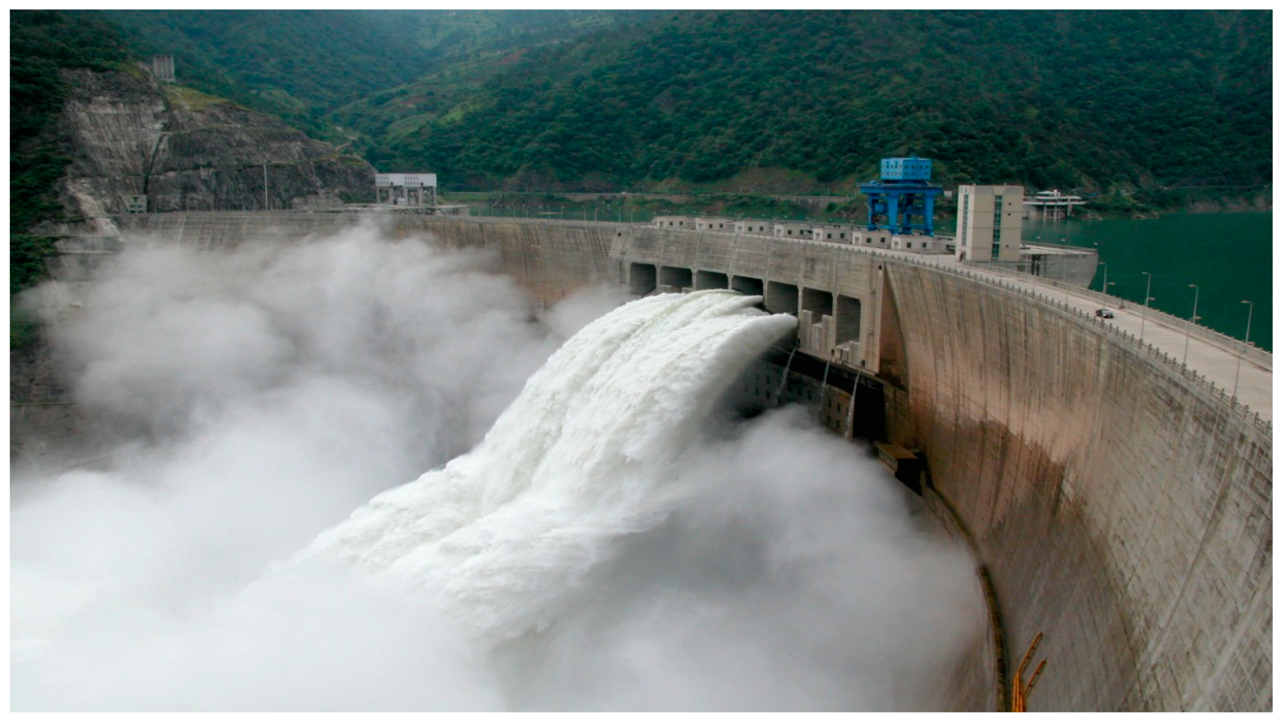
At present, the high dam projects that have been built, are under construction, or are planned in China have the common features of large drops, a narrow river valley, and a large flood discharge flow. The flood discharge energy dissipation mode of the dam body has been mostly adopted by two-jet collisions and downstream water reservoirs, such as Ertan (Figure 1), Xiaowan, Xiluodu, Goupitan, and the Jinping grade I project. Two-jet collisions in air change the motion track of each of the two jets, significantly disperse the water flow, effectively alleviate the dynamic pressure impact of the water flow on the bottom plate of the water cushion reservoir, and have a remarkable energy dissipation effect [1,2,3,4,5,6,7]. However, compared with the traditional energy dissipation method, two-jet collisions in air appear to be a serious problem with regard to flood discharge atomization in the existing engineering examples, which has caused great damage to the normal operation, traffic safety, surrounding environment, and even the stability of the downstream bank slopes. It is necessary to study the spatial distribution characteristics of rainfall intensity in two-jet collisions in air, in order to improve the prediction accuracy of the discharge atomization rain strength and influence range, as well as make a relevant protection classification and protection design scheme in the design planning [8,9,10].
Many former researchers who have studied two-jet collisions in air have focused on the energy dissipation effect of collisions. Xiong [11] introduced the main factors that affect energy dissipation during an in-air collision between the surface and the deep hole. Guo [12] theoretically analyzed the effect of the collision angle on energy dissipation. Using the momentum integral equation of fluid mechanics, Liu [13] derived the related formula of energy dissipation for the collision of two water jets in air in detail, and introduced the concept and calculation method for the energy dissipation rate. Diao [14] studied the relationship between the collision angle, the flow ratio, and the collision energy dissipation effect through model testing, and proposed that the main function of jet collisions is to disperse the water flow. Sun [15] analyzed hydraulic characteristics, such as the energy loss of up- and down-collisions, three-dimensional (3-D) diffusion and leakage collision of the surface, and deep orifice slugs. The 3-D collision velocity, collision efficiency, and collision energy loss were derived using the momentum equation and variation law of the air diffusion width of the water tongue, and the optimal hydraulic conditions for collision were obtained. Sun [16] applied the turbulence jet theory and flow momentum equation, in order to introduce the calculation formula of the collision velocity vector and collision energy dissipation efficiency of the combined water tongue when it collides with the left and right sides of the air.
At present, the research on flood discharge atomization is mainly about ski-jump atomization. Liang [17] proposed a calculation model of atomized water flow, and obtained various calculation formulas and methods in the field of atomized water flow influence. Liu [18,19] studies the diffusion law, velocity distribution, and energy loss of a water jet. According to the prototype observation data of the flood discharge atomization and some experimental data of the model, based on the comprehensive analysis of various factors that affect the atomization range, Li [20] discusses the rough estimation method of the range of the energy dissipation atomization precipitation area. Liu [21,22,23,24] introduces several key problems with regard to the shape and the numerical simulation of atomized flows, such as the jet calculation of the water tongue, collision between the water tongue and the water surface, and calculation of the fog source quantity. By collecting, inducing, and summarizing the partial flood discharge atomization of engineering prototype observation data, Sun [25] found the longitudinal boundary flood discharge atomization average discharge flow, and a good relationship between the water flow velocity and the water entry angle of the water tongue. Based on the dimensional analysis, a method was established to estimate the rainfall intensity, flood discharge atomization, and longitudinal boundary experience relationship. Liu [26] proposed an atomization forecast model based on artificial neural networks. The Monte Carlo method was applied to add the effect of environmental, wind, and topographic factors to the atomization mathematical model of overpass discharge by Lian [27]. Sun [28] revised the resistance coefficient of particles, using the research results of raindrop movement, and obtained the resistance coefficient of the splashing water droplet movement. Then the effect of the diameter of a splashing water droplet on the splashing length is preliminarily discussed, which deepens the understanding of the splashing movement. Using the generalized model test in 2013 by Wang [29]—under different hydraulic conditions, to select a tongue that fell into the water downstream of an atomized water source area of rainfall intensity—the flood discharge atomization fog source area of the plane distribution features was measured and analyzed, to determine the reasons for the formation of different areas around the atomization source and the plane distribution of rainfall intensity. Lian [30] proposes a method to predict the spray atomization of spillage by combining a physical model and theoretical analysis. Zhang [31] experimentally studied the motion track, distribution range, water point shape, and velocity of single-strand jets under different air dosages. Although their methods are accurate in predicting the atomization of a ski-jump flow, they are not good at predicting the atomization of two-jet collisions, which add a collision zone and change the trajectory of two jets. In rocket propulsion, extensive experiments—mostly based on physical model investigations—have been conducted on two-jet collisions, including the liquid membrane [32,33,34,35], droplet size, and velocity distribution [36,37,38,39,40,41].
Most domestic and foreign scholars have focused on the atomization of flood discharge by single-strand pick flows. However, compared with the single-strand pick flow, two-jet collisions in air increase the area of collision atomization, where both range and intensity of the atomization increase. For example, Ertan applied this method to flood discharge and cause landslide by rainfall. Therefore, in this paper, through theoretical analysis and a physical model experiment, we studied the distribution characteristics of rainfall intensity after the collision of two jets, the trajectory lines of the water tongue, and the range of the x-axis after collision for different flow ratios and collision angles.
2. Model Design and Experiment
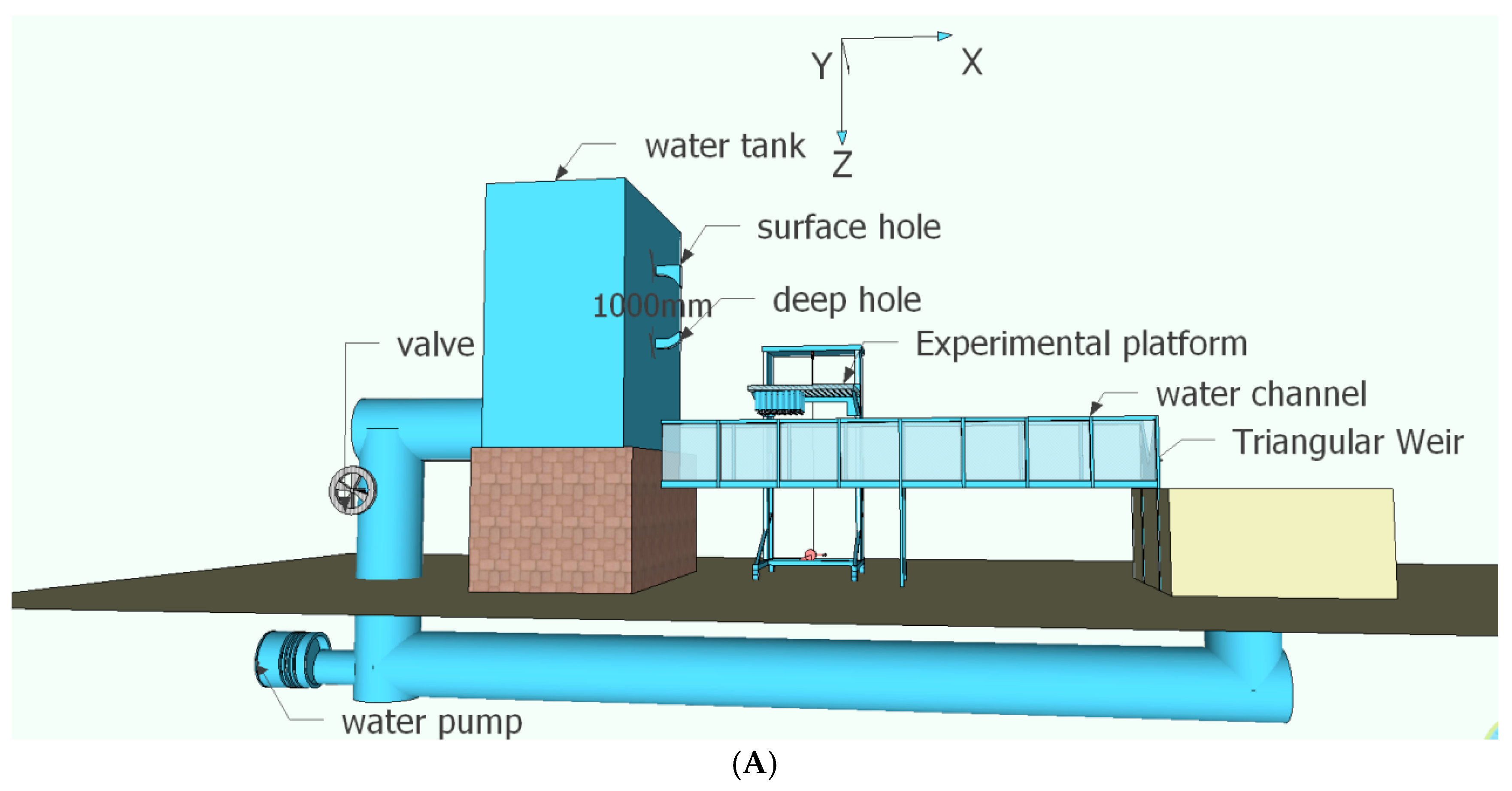
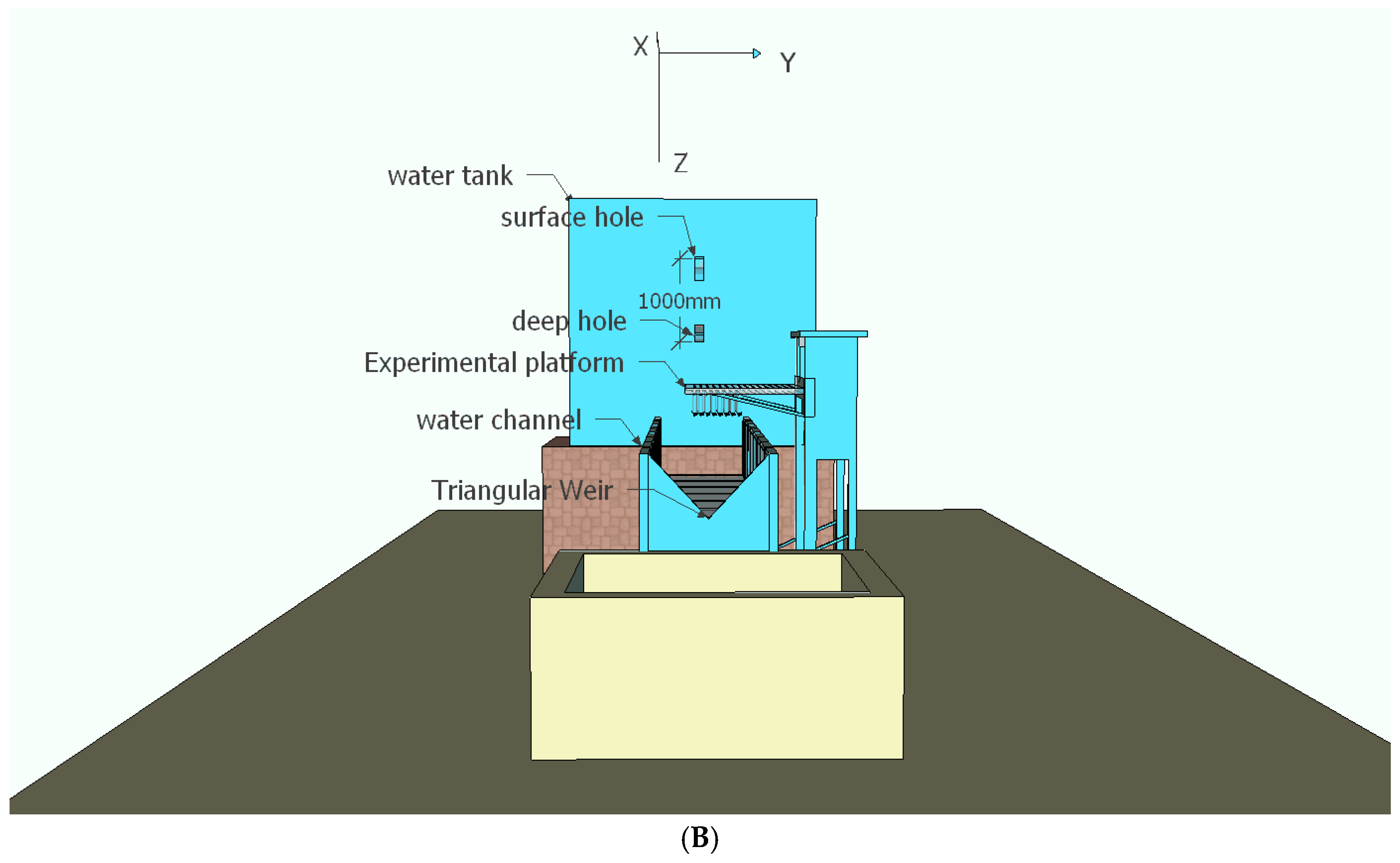
The experiment was conducted in the State Key Laboratory of Hydrodynamics and Mountain River Engineering in Sichuan University. Figure 2 shows the schematic diagram of the model test. The water flux was supplied by a large rectangular tank (width of 4.0 m, length of 4.0 m, and height of 5.0 m). When laying the rainfall receiving platform, we considered the symmetry of the surface and deep hole, and only one side was arranged. Water was fed into the iron box through the pump behind the iron box, and the water level of the iron box was maintained through the valve in order to achieve a stable deep and surface flow.
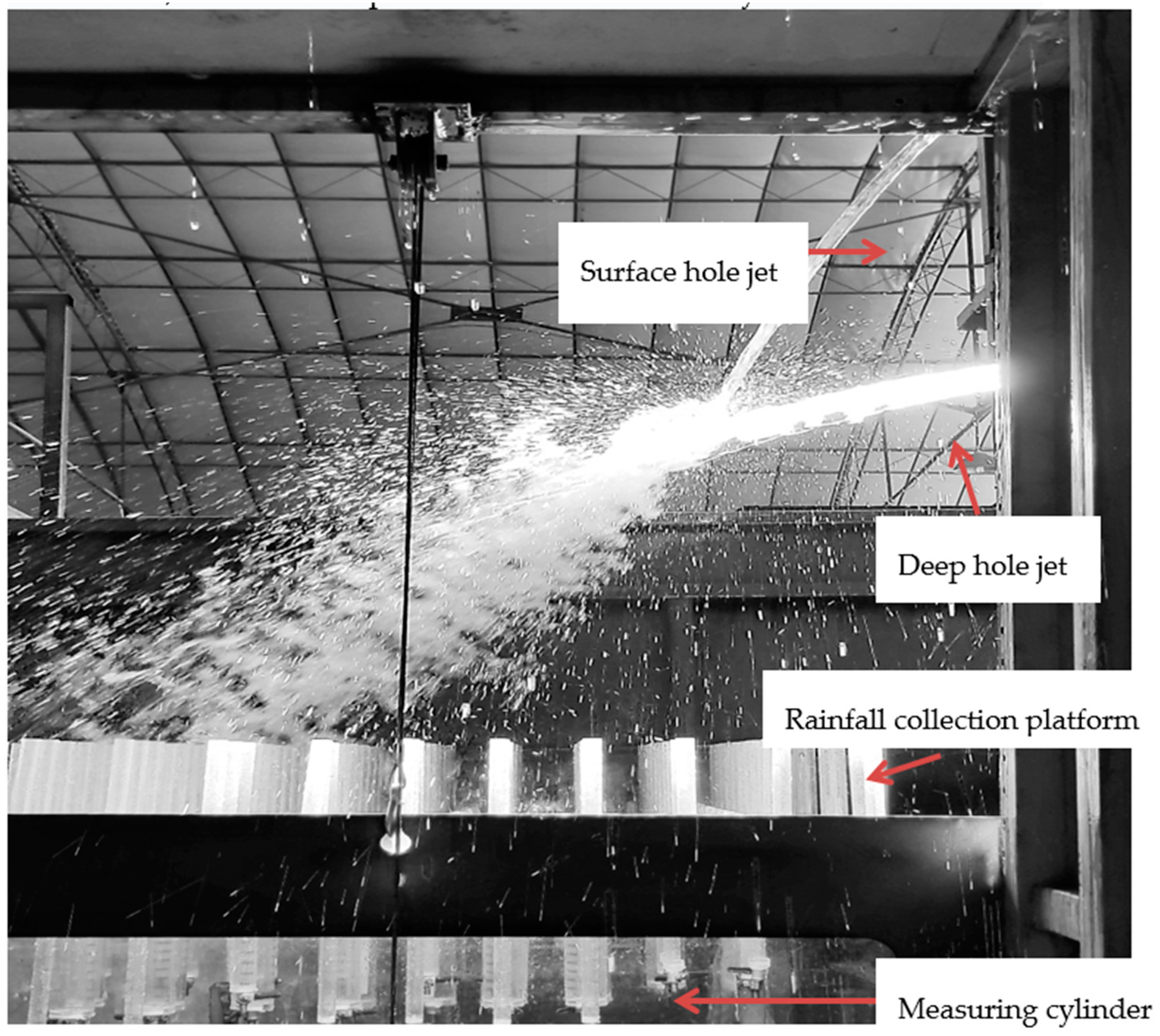
In order to be consistent with the prototype which adopts two-jet collisions in air, this experiment used a constant surface hole angle θ1 (a pitch-down angle of −30°) and adjusted the deep hole pick angle θ2 (0°~45°) to change the collision angle β. The width of the surface deep hole was identical, the height of the deep hole could be adjusted, and the range was 0~5 cm. The maximum single-width flux of the model table hole was 0.1236 m2/s, the maximum single-width flux of the deep hole was 0.1431 m2/s, and the flux was measured by a triangular thin-walled weir (±1%). Four horizontal planes, under the collision points of 36 cm, 56 cm, 76 cm, and 96 cm, were set to measure the rainfall intensity. The platform was supported by a slide rail system, and the accuracy in the vertical platform position was less than 0.5 cm. Table 1 lists 18 working conditions in the experiment, including almost 30,000 measurement points. To obtain the four different sections, we first used image processing to find the collision point, and then adjusted the height of the measuring platform. Detailed visual observations of the collision points were conducted using a Canon EOS80D DSLR camera (Cannon, Chengdu, China).
Rainwater was collected in the horizontal plane (xy plane in Figure 3) at the different elevations below the collision point and 0.15 m above the faceplate. The rainfall collection platform included the movable base, support, and rainfall collection panel, which was made of an organic glass panel and a PVC pipe. In each plane, up to 121 PVC pipes (each with a diameter of 2.0 cm) were used simultaneously to collect rain within a period varying from 60 s to 1000 s, depending on the rain intensity in that region, which was found to be sufficient to ensure stable results. Zhang and Zhu [31] indicated that the measurement error could be ignored with different pipe diameters. In their test, the bottles (25 mL with a bottle-neck diameter of 1.52 cm) were tested to give the same (3% difference) result of rain intensity distribution as those of much larger plastic bottles (250 mL with a bottle-neck diameter of 3.26 cm). To avoid the impact of water splashing on the back of the faceplate, the faceplate was hollow, except for the holes and supporting frames. The lower end of the short pipe, whose range was 15~3000 mL, used a measuring cylinder to collect rainfall. Rainfall intensity varies from point to point, so different cylinders were used. To obtain the whole region’s rainfall intensity, the platform was first placed in one region to collect rainwater, then the entire platform was moved 1.2 m in the longitudinal direction to the next region. To ensure measurement accuracy, two measurements were made in the same working conditions, and the average was taken.
In each test, the total rain flux in the horizontal plane was integrated and compared to the total water flux of the surface and the deep holes. The total water/rain flux Q was calculated from , where I was the measured rain intensity. Comparisons of the integrated values with the water flux at the surface and the deep holes were listed in Table 1. For all tests, the conservation ratio of rain flux on average was 101.4 ± 7.0%. In runs T2-6 and T3-6, the loss of rain flux was slight larger (±9.3%), which may be related to the fact that the rain had a wider range in the test. Hence, the above comparison showed the reliability of the measurements.
3. Experimental Results and Discussion
3.1. Spatial Distribution Characteristics of Rainfall Intensity
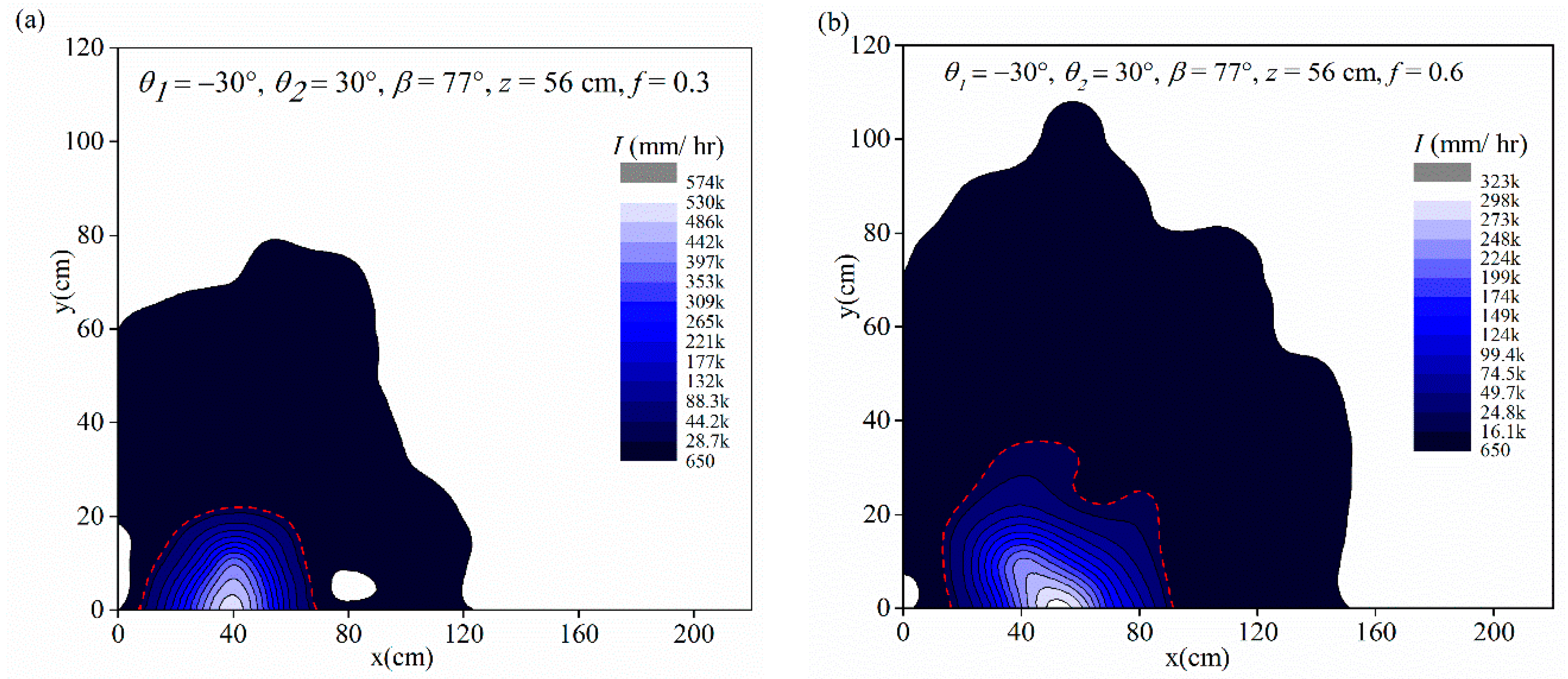
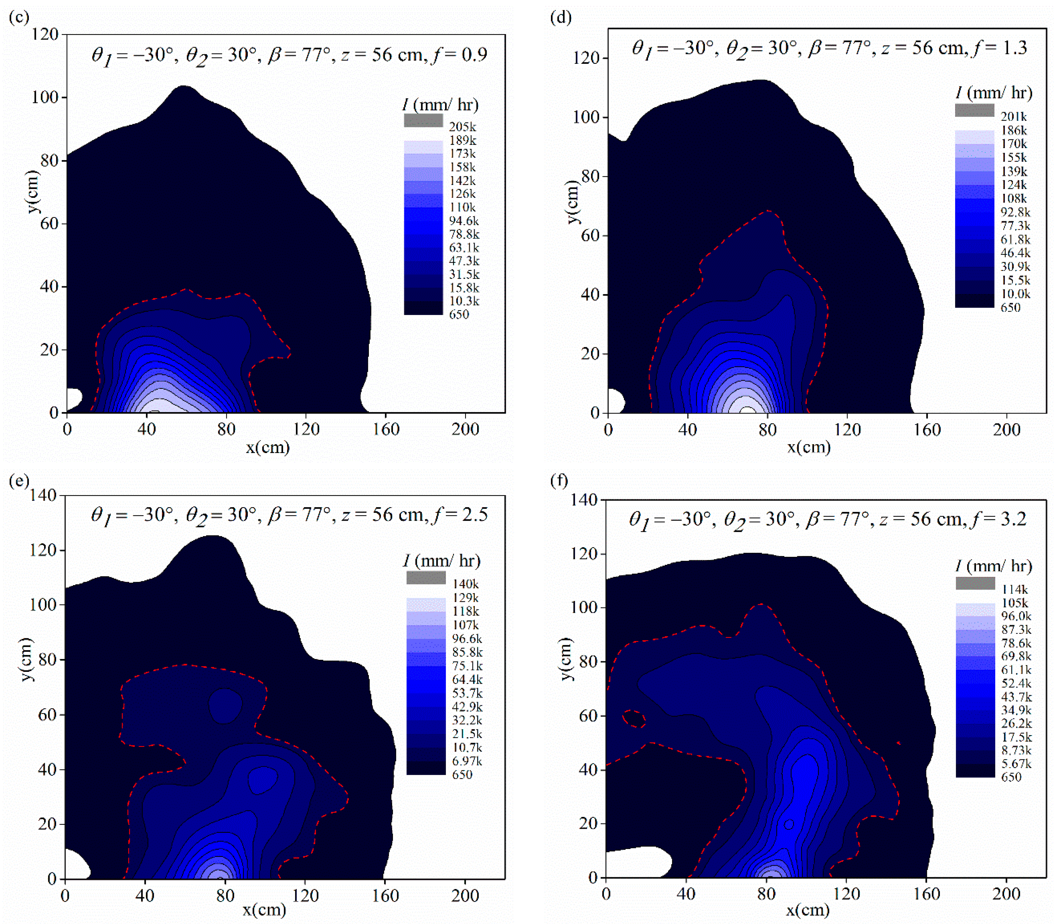
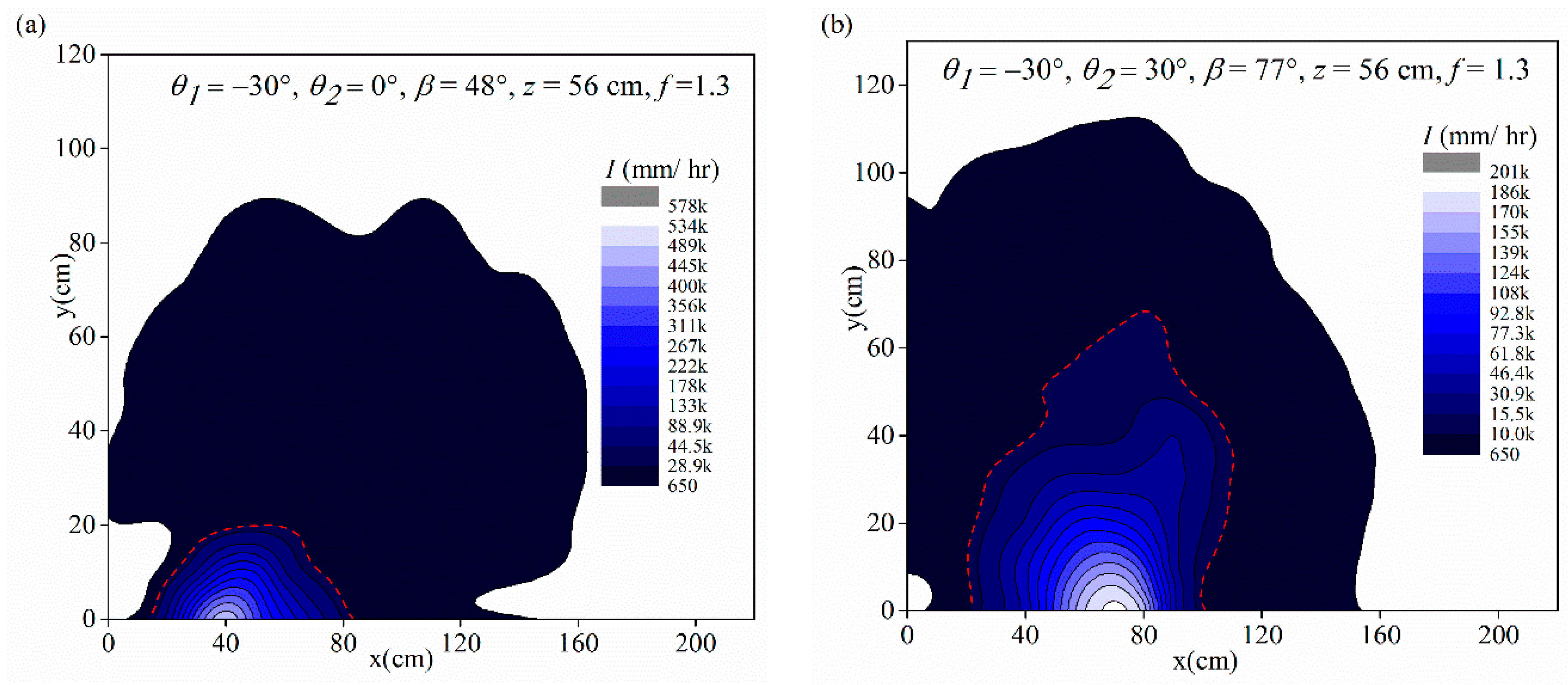
Figure 4, Figure 5 and Figure 6 show the distribution of rainfall intensity for several flow ratios, collision angles, and heights of the rainfall intensity collection platform from the collision point. The rainfall intensity boundary defined 5% of the maximum rainfall intensity under each working condition [31].
In Figure 4, the flow ratios vary, and the height and collision angles from the collision point to the measurement platform are constant. Note that on the section with the same vertical distance from the collision point, the rainfall intensity range showed an increasing trend on the y-axis when the flow ratio increased. On the x-axis, the rainfall intensity range increased first, and subsequently decreased slowly. For f = 0.3, the rainfall intensity range was concentrated in the range 0 cm ≤ x ≤ 22 cm; for f = 0.9, the rainfall intensity range was concentrated in the range of 10 cm ≤ x ≤ 100 cm; while when f = 3.2, the rainfall intensity range was concentrated in the range of 40 cm ≤ x ≤ 115 cm. Under all of the working conditions, the maximum rainfall intensity was on the x-axis.
In Figure 5, the flow ratios and height from the collision point to the measurement platform are constant, and the collision angles vary. Note that with the increase in the collision angle, the rainfall intensity range on the x- and y-axes increased—for example, when β = 48°, Lx = 70 cm, and Ly = 20 cm; when β = 77°, Lx = 108 cm, and Ly = 68 m; when β = 90°, Lx = 163 cm, and Ly = 80 cm. However, the maximum rainfall intensity decreased with the increased collision angle—for example, when β = 48°, Imax = 5.78 × 105 mm/h; and for β = 90°, Imax = 5.78 × 105 mm/h.
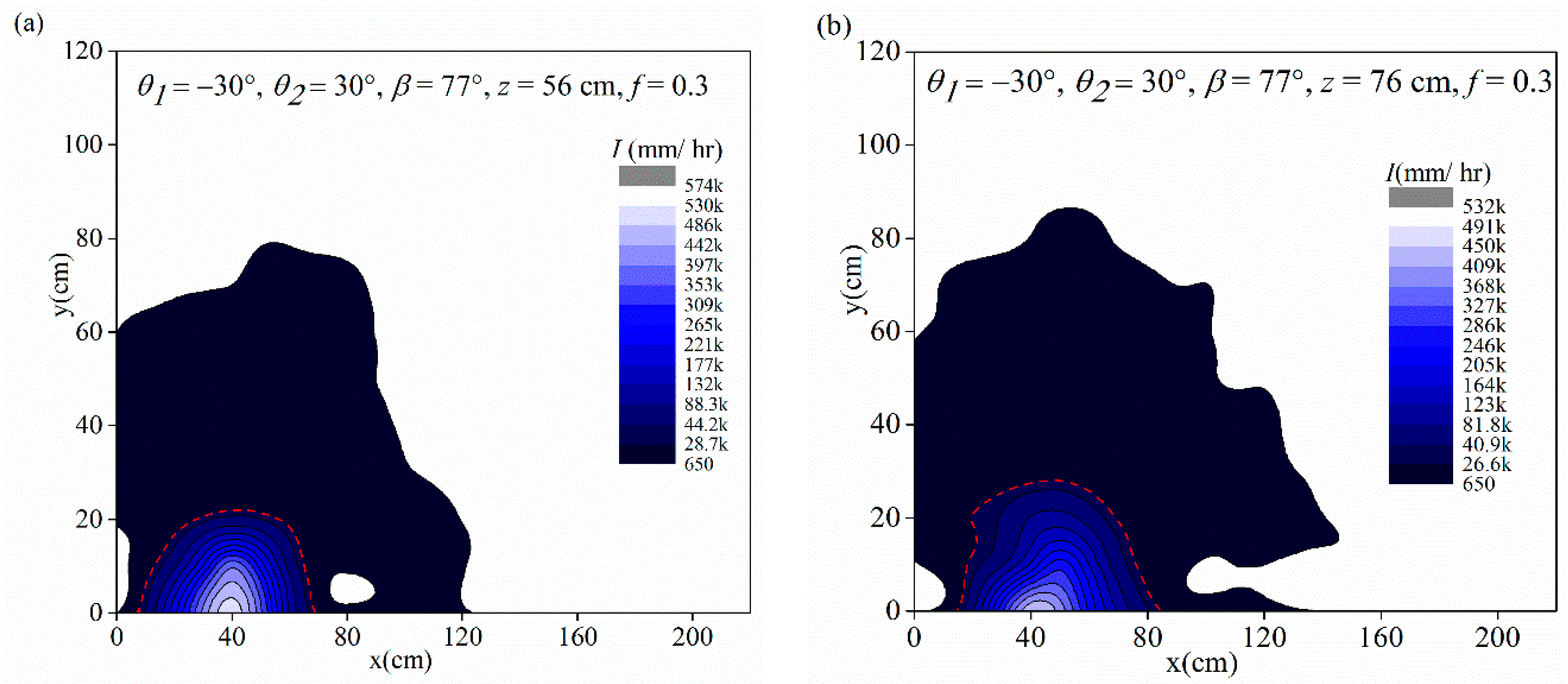
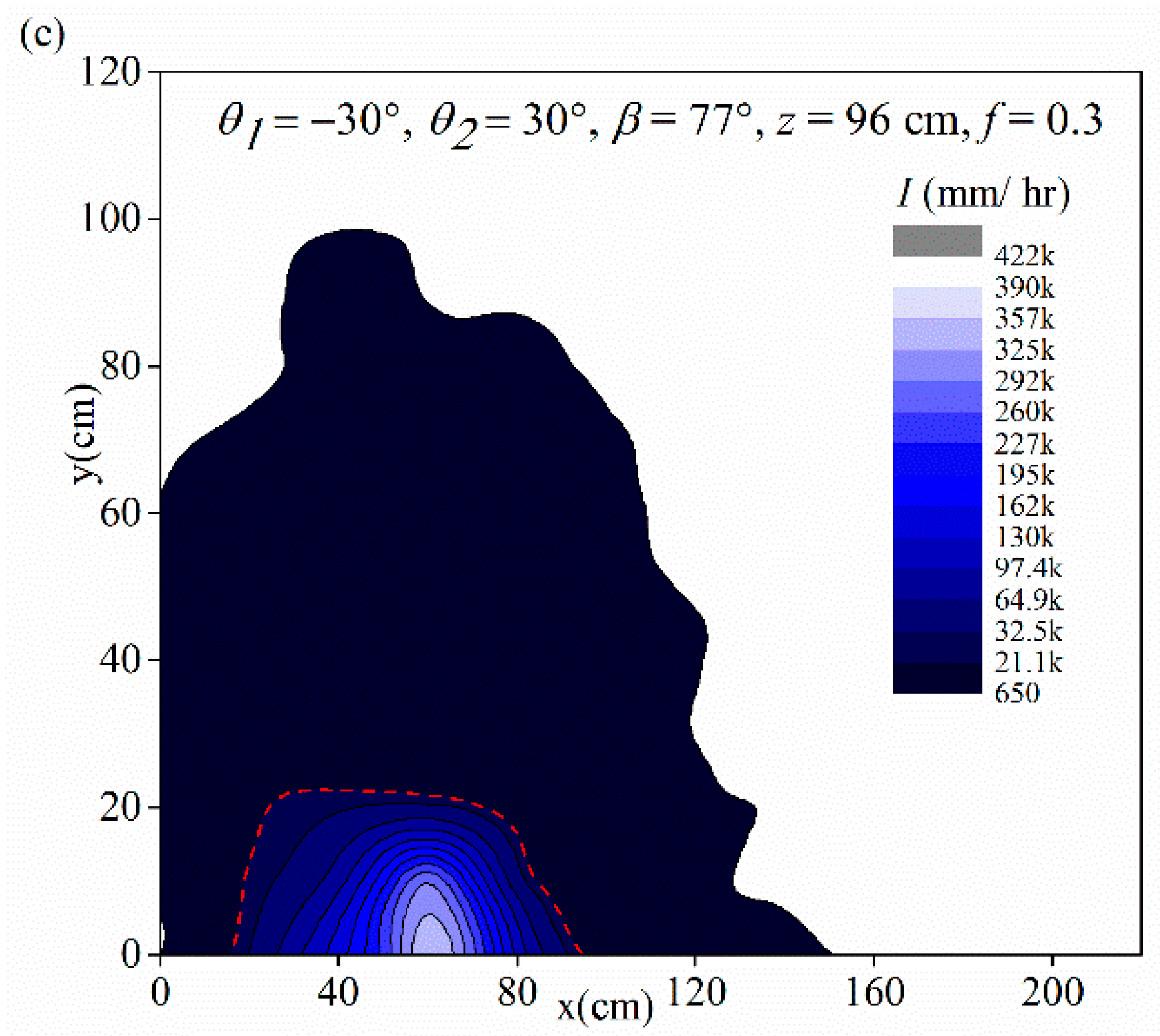
In Figure 6, the flow ratio and collision angle were constant, and the collision point varied from the height of the measurement platform. Note that (1) the range of rainfall intensity on the x- and y-axes gradually increases along the z direction, and (2) the maximum rainfall intensity value continues decreasing. At z = 56 cm, the maximum value is 5.74 × 105 mm/h; at z = 76 cm, the maximum value is 5.32 × 105 mm/h; and at z = 96 cm, the maximum value is 4.22 × 105 mm/h. The maximum value decreases from 5.74 × 105 mm/h to 4.22 × 105 mm/h, which indicates that the maximum rainfall was continuously spreading during the falling process.
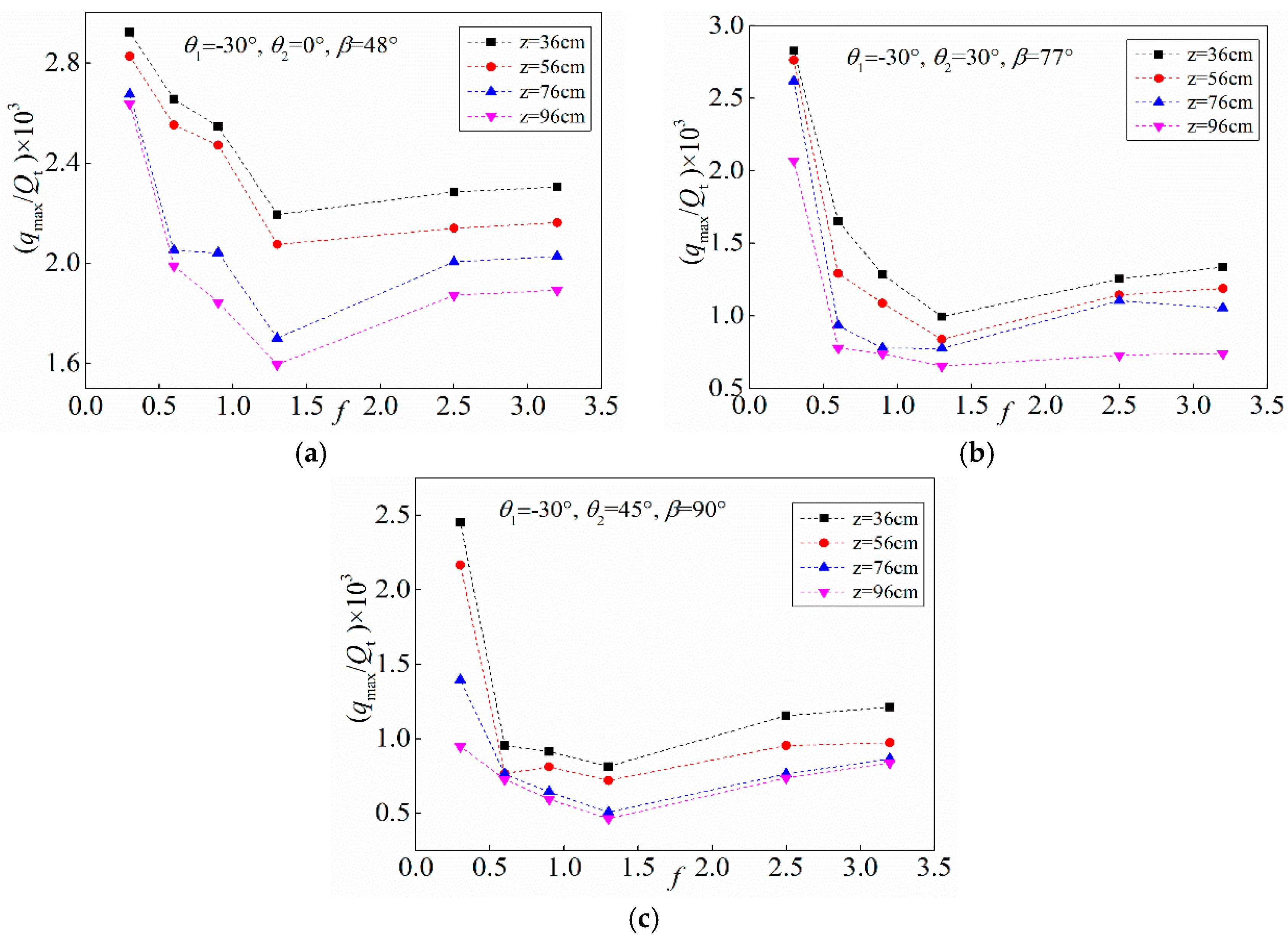
The maximum rainfall of each section (qmax) is shown in Figure 7. Note that (1) the maximum rainfall intensity decreases with an increase in distance of z, (2) qmax sharply decreases for f < 1.4 and slightly increases for f > 1.4, and (3) the results indicated that qmax decreases with an increase of β. In Figure 7a,c, for f = 1.3 and z = 96 cm, qmax/Qt × 103 = 1.6 at β = 48°, while qmax/Qt × 103 decreased to 0.45 at β = 90°, where Qt is the sum flow discharge of surface hole and deep hole outlets.
3.2. Rainfall Intensity Distribution on the x-Axis
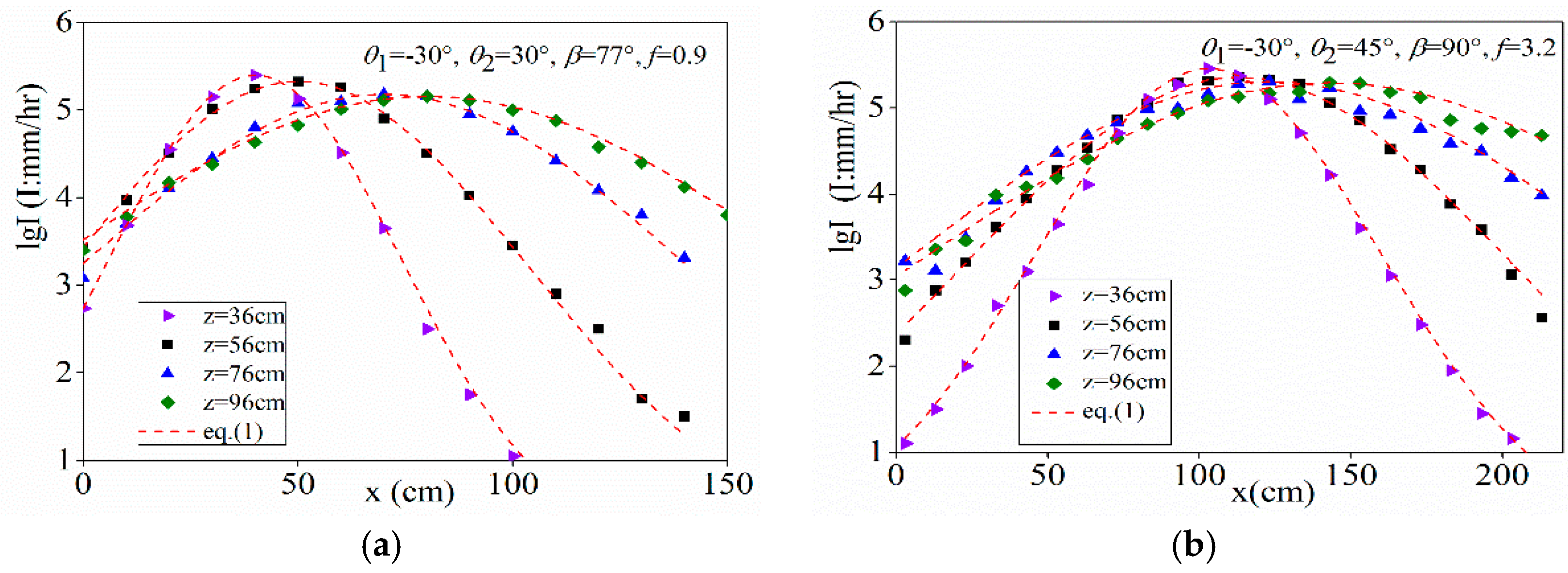
The rainfall intensity distributions on the x-axis are shown in Figure 8. Note that the rainfall intensity data along the x-axis was best correlated with the Gaussian distribution. In addition, the maximum rainfall intensity value gradually decreases with an increase along the z-axis. For example, in Figure 8a, the height of the section increases from 36 cm to 96 cm, and the maximum rainfall intensity value decreases from 2.48 × 105 mm/h to 1.43 × 105 mm/h. With an increase in section height, the rainfall intensity distribution along the x-axis flattens, and the range on the x-axis is bigger.
For two-jet collisions in air on the x- and z-axis, the rainfall intensity distribution along the x-axis after the collision can be expressed by the following formulas (Figure 8):
where I is the rainfall intensity and Imax is the maximum rainfall intensity, is a coefficient.
3.3. Trajectory Line after the Collision on the x-Axis
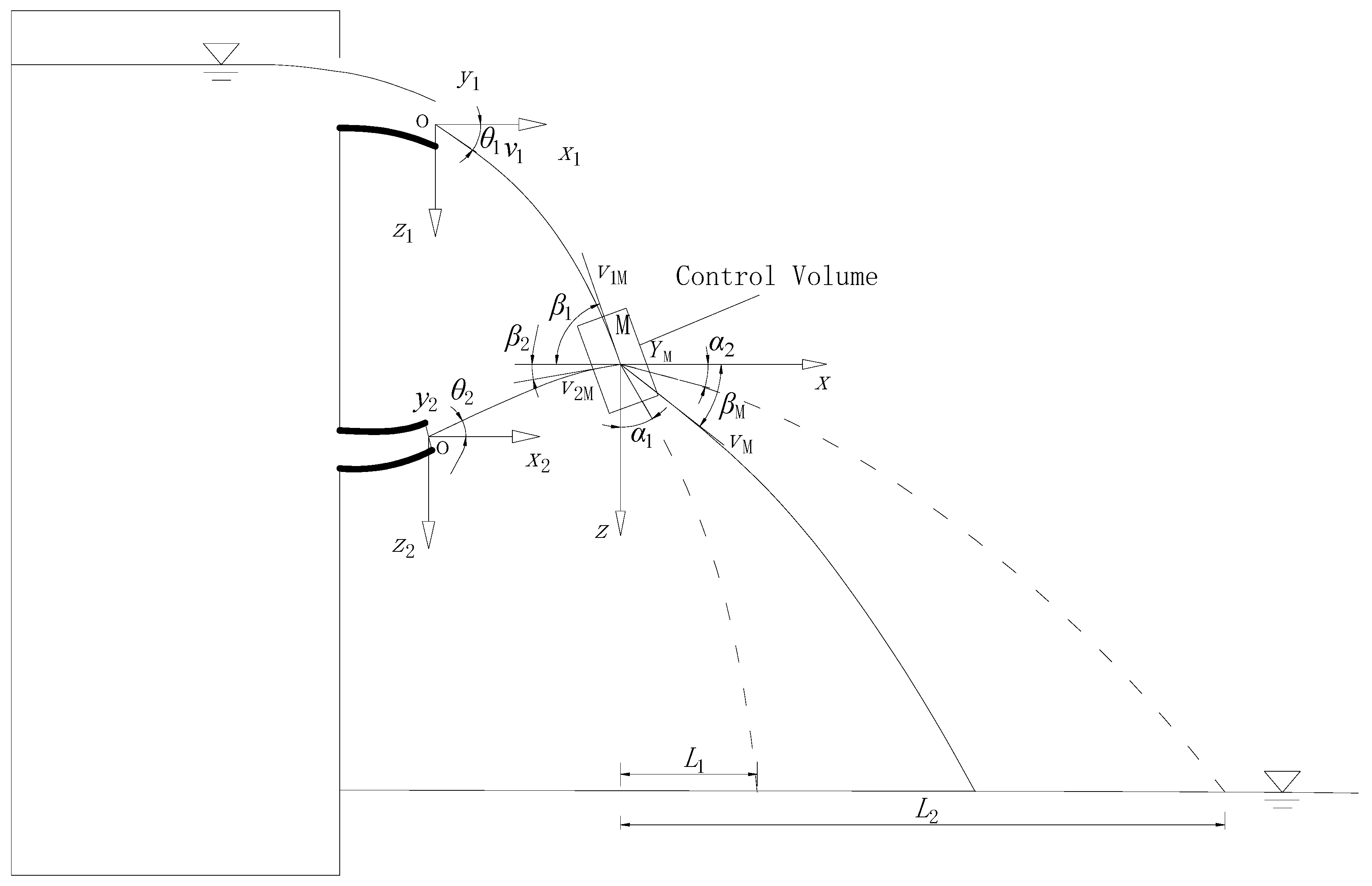
As shown in Figure 9, based on previous research on collision flow [9], the surface water tongue and deep water tongue completely collide in air; then, two water tongues combine and shoot in one direction. V1 is the surface hole water tongue velocity, θ1 is the angle of depression, and q1 is the discharge per unit width; in addition, V1 is the deep hole water tongue velocity, θ2 is the pick angle, and q2 is the discharge per unit width. Two water jets meet at the unit of M. At the confluence, the flow velocity of the upper edge of the water tongue at the confluence is V1M; the angle between the upper edge of the water tongue and the horizontal direction is β1; the flow velocity of the inner edge of the water tongue is V2M; the angle between the inner edge of the water tongue and the horizontal direction is β2; the flow velocity of the mixed water tongue after the phase confluence is VM, and the angle between the water tongue and the horizontal direction is βM.
The spatial position of collision point M can be obtained by calculating the trajectories of the inner edge of the surface-hole jet and outer edge of the deep-hole jet. The trajectories of the deep and surface water tongues were obtained from Equation (3).
where V0 is the initial speed, g is gravity acceleration.
Using the projectile principle, the trajectory equation of the surface water jet was:
where V1 is the surface hole jet initial speed, x1 is the transverse distance, z1 is the vertical distance, .
The energy velocities of V1M and V2M before the impact of the surface water jet and deep water jet became:
where is the velocity coefficient of air resistance (), z1M is the vertical distance from the surface hole to control volume, z2M is the vertical distance from the deep hole to control volume. The control volume was taken around point M, as shown in Figure 9, and the momentum integral equation and continuous equation of fluid mechanics were used.
where is the density of water, and is the external force that acts on the control volume. In the absence of air resistance, βM and VM could be obtained with
with the assumption that V1M = V2M. Thus, Equations (10) and (11) become
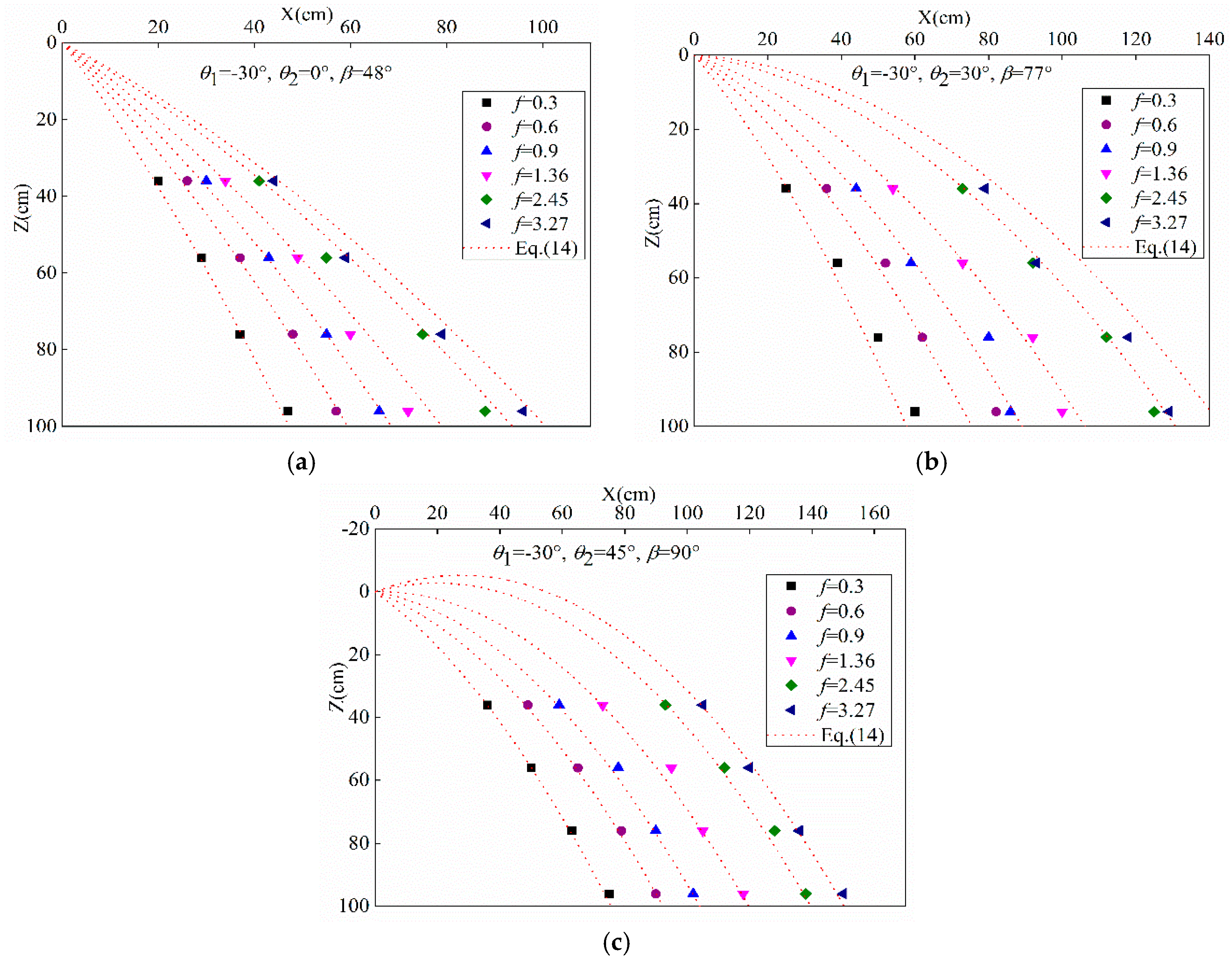
The comparisons of the measured locations of Imax with Equations (12) and (13) are shown in Figure 10, which indicates good agreement.
Based on the above results, we assume that the velocity magnitude was identical in all directions after the collision, but that the directions vary. Therefore, the velocities in all directions were VM. Downstream of the collision, the trajectory boundaries (5% × Imax) are shown in Figure 11. Hence, using Equation (3), α1 and α2 can be obtained—α1 is the angle between the z-axis and the inner edge line, and α2 is the angle between the x-axis and the outer edge line.
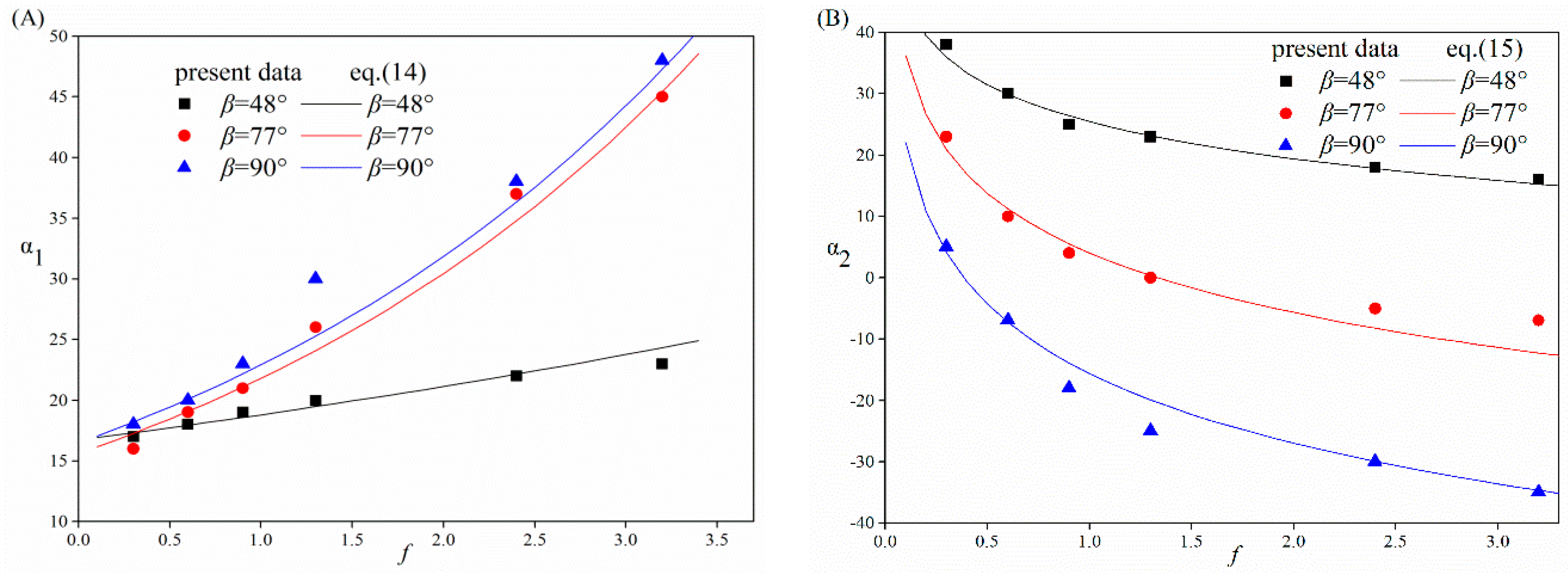
The calculated values of α1 and α2 are shown in Figure 12. Note that (1) with the identical collision angle β, α1 increased, and with the increase in flow ratio, α2 decreased; and (2) with the identical flow ratio, α1 increased with the increase in collision angle β, and α2 decreased with the increase in collision angle β. It can also be seen from Figure 12 that α1 approximately shows exponential growth with the flow ratio, and α2 shows logarithmic growth with the flow ratio. Data analysis indicates that the values of α1 and α2 are obtained as
The computed and measured values correlated to R2 = 0.97 (Figure 12A) and 0.96 (Figure 12B). However, up until now, there was a paucity of information on the rainfall characteristics of the two-jet collisions. This present study provides a new method for understanding the rainfall characteristics of the two-jet collision, which will be useful to extend to other models or even prototypes for further research.
4. Conclusions
In this paper, the flow characteristics of two-jet collisions with different collision angles and flow ratios were investigated systematically by a series of model tests. The present investigation illustrated the development of the spatial distribution of rainfall intensity. Observations indicated that the maximum rainfall intensity sharply decreased with an increase in flow ratio, while the maximum rainfall intensity slightly increased, as the flow ratio was greater than 1.0.
On the x-axis, the distribution of rainfall intensity followed a Gaussian distribution. The range of rainfall intensity tended to reach the maximum for the flow ratio = 1.0. A theoretical equation to compute the locations of maximum rainfall intensity was presented, which is in good agreement with the model tests. The formulas to calculate the boundary lines of the x-axis were proposed. The present analysis was based upon experiments performed in a model with 48° < β < 90°, 0.3 < f < 3.2, and 36 cm < z < 96 cm. The rainfall intensity distributions on the y-axis will be further studied.
Author Contributions
Conceptualization, H.Y. and W.X.; Methodology, W.X.; Software, Validation, H.Y.; W.X. and R.L.; Formal Analysis, H.Y.; Experiment, H.Y., Y.F., Y.H.; Writing-Original Draft Preparation, H.Y.; Writing-Review & Editing, H.Y.; Supervision, W.X.; Project Administration, W.X.; Funding Acquisition, W.X.
Funding
This work was supported by the National Key Research and Development Program of China (Grant No. 2016YFC0401707) and National Natural Science Foundation of China (Grant 51609162 and Grant 51409181).
Conflicts of Interest
The authors declare no conflicts of interest.
References
- Li, N.-W. Study on the Non-Collision Way of Flood Discharge and Energy Dissipation in High Arch Dams with Contracting Spillways and Middle Level Outlets; Sichuan University: Chengdu, China, 2008. [Google Scholar]
- Li, N.-W.; Xu, W.-L.; Zhou, M.-L.; Tian, Z. Experimental study on energy dissipation of flood discharge in high arch dams without impact of jets in air. J. Hydraul. Eng. 2008, 39, 927–933. [Google Scholar]
- Shuangke, S. Summary of research on flood discharge and energy dissipation of high dams in China. J. China Inst. Water Resour. Hydropower Res. 2009, 7, 89–95. [Google Scholar]
- Bai, R.; Zhang, F.; Liu, S.; Wang, W. Air concentration and bubble characteristics downstream of a chute aerator. Int. J. Multiph. Flow 2016, 87, 156–166. [Google Scholar] [CrossRef]
- Bai, R.; Liu, S.; Tian, Z.; Wang, W.; Zhang, F. Experimental investigations on air-water flow properties of offse-aerator. J. Hydraul. Eng. 2017, 144, 04017059. [Google Scholar] [CrossRef]
- Li, S.; Zhang, J.; Xu, W.; Chen, J.; Peng, Y. Evolution of Pressure and Cavitation on Side Walls Affected by Lateral Divergence Angle and Opening of Radial Gate. J. Hydraul. Eng. 2016, 142, 05016003. [Google Scholar] [CrossRef]
- Bai, Z.; Peng, Y.; Zhang, J. Three-dimensional turbulence simulation of flow in a V-shaped stepped spillway. J. Hydraul. Eng. 2017, 143, 06017011. [Google Scholar] [CrossRef]
- Huang, G.; Wu, S.; Chen, H. Model test studies of atomized flow for high dams. Hydro-Sci. Eng. 2008, 2008, 91–94. [Google Scholar]
- Xue, L.-F. Influence of atomization on environment during flood discharge from dam and reducing measures. Sichuan Water Power 2005, 24, 104–107. [Google Scholar]
- Bai, R.; Liu, S.; Tian, Z.; Wang, W.; Zhang, F. Experimental investigation of the dissipation rate in a chute aerator flow. Exp. Therm. Fluid Sci. 2019, 101, 201–208. [Google Scholar] [CrossRef]
- Xiong, X.-L.; Ge, G. The collision energy dissipation between surface hole’s water tongue and middle hole’s water tongue of Ertan hydropower station. J. Hydropower Eng. Res. 1991, 1–10. (In Chinese) [Google Scholar]
- Chi-gong, G.Y.W. An optimal research on the energy dissipation by collision of two free jets in ertan hydroelectric plant. J. Chengdu Univ. Sci. Technol. 1992, 18, 17–24. [Google Scholar]
- Liu, P.; Dong, J.; Liu, Y. Computation of energy dissipation for impact of two jets in air. J. Hydraul. Eng. 1995, 7, 38–44. [Google Scholar]
- Diao, M.J.; Yang, Y.Q. Experimental study on two jets impact in air for energy dissipation. J. Sichuan Univ. (Eng. Sci. Ed.) 2002, 34, 13–15. [Google Scholar]
- Sun, J.; Li, Y.-Z. Hydraulic characteristics of water jets by air-collision in lateral direction and estimation on limiting riverbed scour. Chin. J. Appl. Mech. 2004, 21, 134–137. [Google Scholar]
- Sun, J.; Li, Y.-Z.; Yu, C.-Z. Limiting scour depth by the interaction of water jets from surface outlets with jets from mid-level outlets in high arch dams. J. Tsinghua Univ. (Sci. Technol.) 2002, 42, 564–568. [Google Scholar]
- Liang, Z.-C. A Computation Model for Atomization Flow. J. Hydrodyn. 1992, 7, 247–255. [Google Scholar]
- Liu, X.-L.; Zhang, W. The investigation of dynamic characteristics of jet-flow in open air. J. Hydroelectr. Eng. 1988, 2, 46–54. (In Chinese) [Google Scholar]
- Liu, X.-L.; Liu, J. Experiment study on the diffusion and aeration of three-dimensional jet. J. Hydraul. Eng. 1989, 11, 9–17. (In Chinese) [Google Scholar]
- Li, W.-X.; Wang, W.; Xu, W.-L.; Diao, M.-J. A rough method to calculate the range of atomized flow caused by jet impact. J. Sichuan Union Univ. (Eng. Sci. Ed.) 1999, 3, 17–23. [Google Scholar]
- Liu, S.-H.; Liang, Z.-C. On atomizing problems by jumping jet in hydropower station at narrow and deep valley. J. Wuhan Univ. Hydraul. Electr. Eng. 1997, 30, 6–9. [Google Scholar]
- Liu, S.-H.; Qu, B. Investigation on splash length of aerated jet. J. Wuhan Univ. Hydraul. Electr. Eng. 2003, 36, 5–8. [Google Scholar]
- Liu, S.-H. Study of the atomized flow in hydraulic engineering. J. Hydrodyn. 1999, 2, 77–83. [Google Scholar]
- Liu, S.-H.; Yin, S.-R.; Luo, Q.-S. Numerical simulation of atomized flow diffusion in deep and narrow goeges. Conf. Glob. Chin. Scholar Hydrodyn. 2006, 18, 515–518. [Google Scholar]
- Sun, S.-K.; Liu, Z.-P. Longitudinal range of atomized flow forming by discharge of spillways and outlet works in hydropower stations. J. Hydraul. Eng. 2003, 34, 53–58. [Google Scholar]
- Liu, H.-T.; Sun, S.-K.; Liu, Z.-P.; Wang, X.-S. Atomization prediction based on artificial neural networks for flood releasing of high dams. J. Hydraul. Eng. 2005, 36, 1241–1245. [Google Scholar]
- Lian, J.-J.; Liu, F.; Huang, C.-Y. Numerical study on effects of environmental wind and terrain on spray caused by jet from flip bucket. J. Hydraul. Eng. 2005, 36, 1147–1152. [Google Scholar]
- Sun, X.-F.; Liu, S.-H. Investigation on the motion of splash droplets in atomized flow. J. Hydrodyn. 2008, 23, 61–66. [Google Scholar]
- Wang, S.-Y.; Chen, D.; Hou, D.-M. Experimental Research on the Rainfall intensity in the Source Area of Flood Discharge Atomization. J. Yangtze River Sci. Res. Inst. 2013, 30, 70–74. [Google Scholar]
- Lian, J.-J.; Li, C.-Y.; Liu, F.; Wu, S.-Q. A prediction method of flood discharge atomization for high dams. J. Hydraul. Res. 2014, 52, 274–282. [Google Scholar] [CrossRef]
- Zhang, W.; Zhu, D. Far-field properties of aerated water jets in air. Int. J. Multiph. Flow 2015, 76, 158–167. [Google Scholar] [CrossRef]
- Taylor, G. Formation of thin flat sheets of water. Proc. R. Soc. 1960, 259, 1–17. [Google Scholar] [CrossRef]
- Dombrowski, N.; Hooper, P.C. A study of the sprays formed by impinging jets in laminar and turbulent flow. J. Fluid Mech. 1963, 18, 392–440. [Google Scholar] [CrossRef]
- Anderson, W.E.; Ryan, H.M.; Pal, S.; Santoro, R.J. Fundamental studies of impinging liquid jets. In Proceedings of the 30th AIAA, Aerospace Sciences Meeting and Exhibit, Reno, NV, USA, 6–9 January 1992; Volume 1, pp. 6–9. [Google Scholar]
- Ibrahim, E.A.; Przekwas, A.J. Impinging jets atomization. Phys. Fluids Fluid Dyn. 1991, 3, 2981–2987. [Google Scholar] [CrossRef]
- Choo, Y.J.; Kang, B.S. Parametric study on impinging-jet liquid sheet thickness distribution using an interferometric method. Exp. Fluids 2001, 31, 56–62. [Google Scholar] [CrossRef]
- Choo, Y.J.; Kang, B.S. The velocity distribution of the liquid sheet formed by two low-speed impinging jets. Phys. Fluids 2002, 14, 622–627. [Google Scholar] [CrossRef]
- Couto, H.S.; Bastos-Netto, D. Modeling droplet size distribution from impinging jets. J. Propul. Power 1989, 7, 654–656. [Google Scholar] [CrossRef]
- Choo, Y.J.; Kang, B.S. A study on the velocity characteristics of the liquid elements produced by two impinging jets. Exp. Fluids 2003, 34, 655–661. [Google Scholar] [CrossRef]
- Lee, C.H. An experimental study on the distribution of the drop size and velocity in asymmetric impinging jet sprays. J. Mech. Sci. Technol. 2008, 22, 608. [Google Scholar] [CrossRef]
- Fore, L.B.; Dukler, A.E. The distribution of drop size and velocity in gas-liquid annular flow. Int. J. Multiph. Flow 1995, 21, 137–149. [Google Scholar] [CrossRef]
Figure 1.
Simultaneous discharge of the surface and the deep hole of the Ertan hydropower station in 2010.
Figure 1.
Simultaneous discharge of the surface and the deep hole of the Ertan hydropower station in 2010.

Figure 2.
(A) Experiment layout: side view; (B) experiment layout: front view.


Figure 3.
Rainfall collection platform in 2017.

Figure 4.
Rainfall intensity distribution at different flow ratios on the x-o-y measuring platform. (a) θ1 = −30°, θ2 = 30°, β = 77°, z = 56 cm, and f = 0.3; (b) θ1 = −30°, θ2 = 30°, β = 77°, z = 56 cm, and f = 0.6; (c) θ1 = −30°, θ2 = 30°, β = 77°, z = 56 cm, and f = 0.9; (d) θ1 = −30°, θ2 = 30°, β = 77°, z = 56 cm, and f = 1.3; (e) θ1 = −30°, θ2 = 30°, β = 77°, z = 56 cm, and f = 2.5; (f) θ1 = −30°, θ2 = 30°, β = 77°, z = 56 cm, and f = 3.2.


Figure 5.
Rainfall intensity distribution at different collision angles on the x-o-y measuring platform. (a) θ1 = −30°, θ2 = 0°, β = 48°, z = 56 cm, and f = 1.3; (b) θ1 = −30°, θ2 = 30°, β = 77°, z = 56 cm, and f = 1.3; (c) θ1 = −30°, θ2 = 45°, β = 90°, z = 56 cm, and f = 1.3.
Figure 5.
Rainfall intensity distribution at different collision angles on the x-o-y measuring platform. (a) θ1 = −30°, θ2 = 0°, β = 48°, z = 56 cm, and f = 1.3; (b) θ1 = −30°, θ2 = 30°, β = 77°, z = 56 cm, and f = 1.3; (c) θ1 = −30°, θ2 = 45°, β = 90°, z = 56 cm, and f = 1.3.


Figure 6.
Rainfall intensity distribution at different section heights on the x-o-y measuring platform. (a) θ1 = −30°, θ2 = 30°, β = 77°, z = 56 cm, and f = 0.3; (b) θ1 = −30°, θ2 = 30°, β = 77°, z = 76 cm, and f = 0.3; (c) θ1 = −30°, θ2 = 30°, β = 77°, z = 96 cm, and f = 0.3.
Figure 6.
Rainfall intensity distribution at different section heights on the x-o-y measuring platform. (a) θ1 = −30°, θ2 = 30°, β = 77°, z = 56 cm, and f = 0.3; (b) θ1 = −30°, θ2 = 30°, β = 77°, z = 76 cm, and f = 0.3; (c) θ1 = −30°, θ2 = 30°, β = 77°, z = 96 cm, and f = 0.3.


Figure 7.
The maximum rainfall varies with the collision angles and flow ratios at different sections. (a) θ1 = −30°, θ2 = 0°, and β = 48°; (b) θ1 = −30°, θ2 = 30°, and β = 77°; (c) θ1 = −30°, θ2 = 45°, and β = 90°.
Figure 7.
The maximum rainfall varies with the collision angles and flow ratios at different sections. (a) θ1 = −30°, θ2 = 0°, and β = 48°; (b) θ1 = −30°, θ2 = 30°, and β = 77°; (c) θ1 = −30°, θ2 = 45°, and β = 90°.

Figure 8.
Rainfall intensity distributions along the x-axis and comparison with Equations (1) and (2). (a) θ1 = −30°, θ2 = 30°, β = 77°, and f = 0.9; (b) θ1 = −30°, θ2 = 45°, β = 90°, and f = 3.2.
Figure 8.
Rainfall intensity distributions along the x-axis and comparison with Equations (1) and (2). (a) θ1 = −30°, θ2 = 30°, β = 77°, and f = 0.9; (b) θ1 = −30°, θ2 = 45°, β = 90°, and f = 3.2.

Figure 9.
Schematic diagram of the collision between the surface-hole jet and the deep-hole jet in air.
Figure 9.
Schematic diagram of the collision between the surface-hole jet and the deep-hole jet in air.

Figure 10.
Comparison of experimental and calculated values of the maximum rainfall intensity points. (a) θ1 = −30°, θ2 = 0°, and β = 48°; (b) θ1 = −30°, θ2 = 30°, and β = 77°; (c) θ1 = −30°, θ2 = 45°, and β = 90°.
Figure 10.
Comparison of experimental and calculated values of the maximum rainfall intensity points. (a) θ1 = −30°, θ2 = 0°, and β = 48°; (b) θ1 = −30°, θ2 = 30°, and β = 77°; (c) θ1 = −30°, θ2 = 45°, and β = 90°.

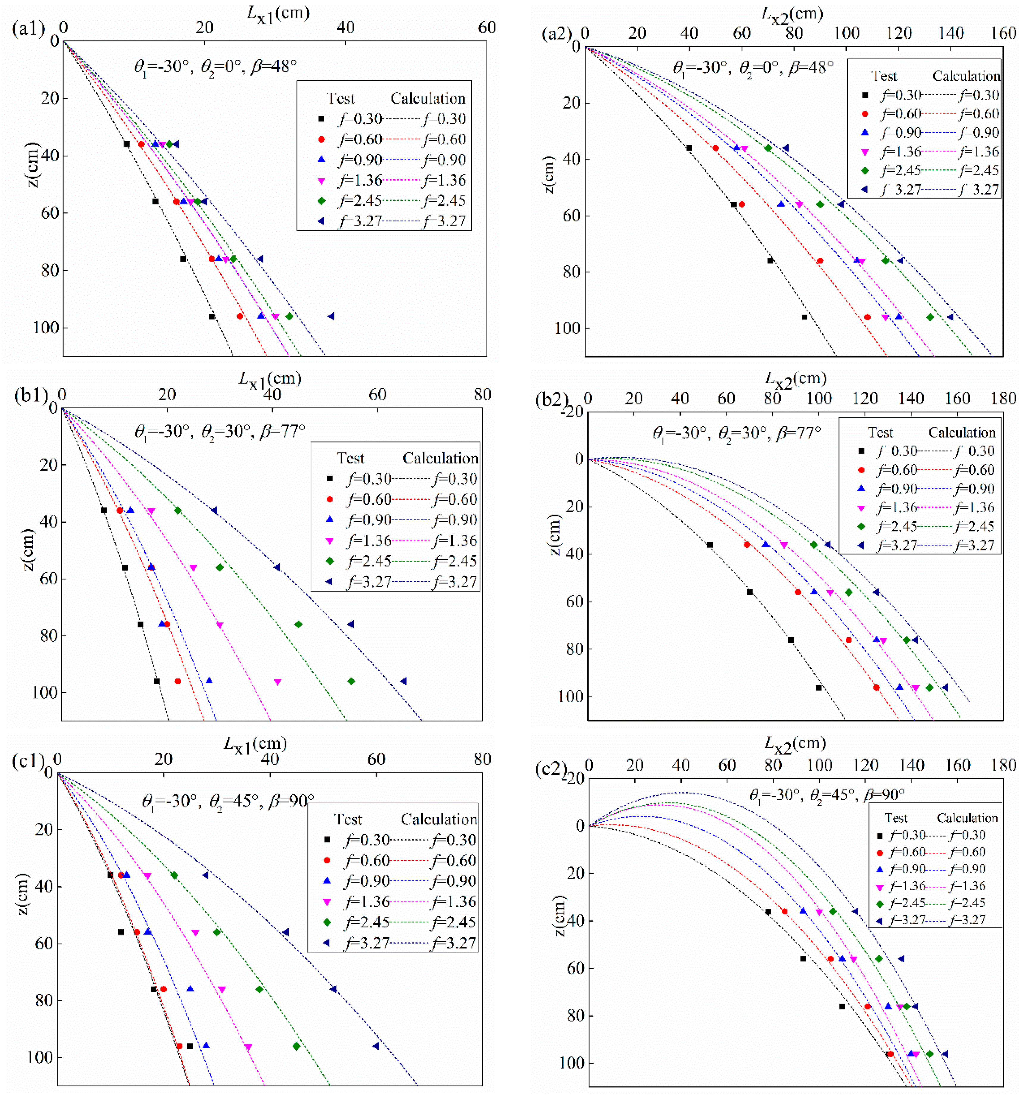
Figure 11.
Comparison of the experimental and calculated values of LX1 and LX2. LX1 is the distance of inner edge water tongue in x axis, LX2 is the distance of outer edge water tongue in x axis. (a1) θ1 = −30°, θ2 = 0°, and β = 48°; (a2) θ1 = −30°, θ2 = 0°, and β = 48°; (b1) θ1 = −30°, θ2 = 30°, and β = 77°; (b2) θ1 = −30° and θ2 = 30°; (c1) θ1 = −30°, θ2 = 45°, and β = 90°; (c2) θ1 = −30°, θ2 = 45°, and β = 90°.

Figure 12.
Comparison of the values obtained from Equations (14) and (15) with the present data. (A) Inner angle of α1, and (B) outer angle of α2.
Figure 12.
Comparison of the values obtained from Equations (14) and (15) with the present data. (A) Inner angle of α1, and (B) outer angle of α2.


Table 1.
Working conditions in experiments.
| Run | θ1 (°) | θ2 (°) | qm (m2/s) | qc (m2/s) | f | Q × 2/(qm + qc) |
|---|---|---|---|---|---|---|
| T1-1 | −30 | 0 | 0.0373 | 0.1236 | 0.3 | 103% |
| T1-2 | −30 | 0 | 0.0745 | 0.1236 | 0.6 | 95% |
| T1-3 | −30 | 0 | 0.0727 | 0.0800 | 0.9 | 102% |
| T1-4 | −30 | 0 | 0.1091 | 0.0800 | 1.3 | 104% |
| T1-5 | −30 | 0 | 0.1073 | 0.0436 | 2.5 | 98% |
| T1-6 | −30 | 0 | 0.1427 | 0.0436 | 3.2 | 104% |
| T2-1 | −30 | 30 | 0.0373 | 0.1236 | 0.3 | 95% |
| T2-2 | −30 | 30 | 0.0745 | 0.1236 | 0.6 | 110% |
| T2-3 | −30 | 30 | 0.0727 | 0.0800 | 0.9 | 102% |
| T2-4 | −30 | 30 | 0.1091 | 0.0800 | 1.3 | 105% |
| T2-5 | −30 | 30 | 0.1073 | 0.0436 | 2.5 | 103% |
| T2-6 | −30 | 30 | 0.1427 | 0.0436 | 3.2 | 92% |
| T3-1 | −30 | 45 | 0.0373 | 0.1236 | 0.3 | 111% |
| T3-2 | −30 | 45 | 0.0745 | 0.1236 | 0.6 | 94% |
| T3-3 | −30 | 45 | 0.0727 | 0.0800 | 0.9 | 103% |
| T3-4 | −30 | 45 | 0.1091 | 0.0800 | 1.3 | 106% |
| T3-5 | −30 | 45 | 0.1073 | 0.0436 | 2.5 | 108% |
| T3-6 | −30 | 45 | 0.1427 | 0.0436 | 3.2 | 111% |
qm is the flow discharge per unit width of deep hole. qc is the flow discharge per unit width of surface hole. f is the ratio of deep hole flow to surface hole flow, that is f = qm/qc. Q is the integral of measurement value.
© 2018 by the authors. Licensee MDPI, Basel, Switzerland. This article is an open access article distributed under the terms and conditions of the Creative Commons Attribution (CC BY) license (http://creativecommons.org/licenses/by/4.0/).
Share and Cite
MDPI and ACS Style
Yuan, H.; Xu, W.; Li, R.; Feng, Y.; Hao, Y. Spatial Distribution Characteristics of Rainfall for Two-Jet Collisions in Air. Water 2018, 10, 1600. https://doi.org/10.3390/w10111600
AMA Style
Yuan H, Xu W, Li R, Feng Y, Hao Y. Spatial Distribution Characteristics of Rainfall for Two-Jet Collisions in Air. Water. 2018; 10(11):1600. https://doi.org/10.3390/w10111600
Chicago/Turabian StyleYuan, Hao, Weilin Xu, Rui Li, Yanzhang Feng, and Yafeng Hao. 2018. "Spatial Distribution Characteristics of Rainfall for Two-Jet Collisions in Air" Water 10, no. 11: 1600. https://doi.org/10.3390/w10111600
Note that from the first issue of 2016, this journal uses article numbers instead of page numbers. See further details here.