The Influence of Hyporheic Exchange on Water Temperatures in a Headwater Stream


Natural Resources Management and Environmental Sciences Department, California Polytechnic State University, San Luis Obispo, CA 93407, USA
*
Author to whom correspondence should be addressed.
Water 2018, 10(11), 1615; https://doi.org/10.3390/w10111615
Submission received: 10 October 2018
/
Revised: 7 November 2018
/
Accepted: 7 November 2018
/
Published: 9 November 2018
(This article belongs to the Section Water Quality and Contamination)
Abstract
:A headwater stream in coastal California was used to evaluate the temperature response of effective shade reduction. Spatial distribution of stream water temperatures for summer low-flow conditions (<0.006 m3 s−1) were highly correlated with net radiation and advective heat transfers from hyporheic exchange and subsequent streambed conduction. Using a heat budget model, mean maximum stream water temperatures were predicted to increase by 1.7 to 2.2 °C for 50% and 0% effective shade scenarios, respectively, at the downstream end of a 300 m treatment reach. Effects on mean maximum stream water temperature changes, as water flowed downstream through a 500 m shaded reach below the treatment reach, were reduced by 52 to 30% from the expected maximum temperature increases under the 50% and 0% effective shade scenarios, respectively. Maximum stream water temperature change predicted by net radiation heating alone was greater than measured and heat-budget-estimated temperatures. When the influence of hyporheic water exchange was combined with net radiation predictions, predicted temperatures were similar to measured and heat-budget-predicted temperatures. Results indicate that advective heat transfers associated with hyporheic exchange can promote downstream cooling following stream water temperature increases from shade reduction in a headwater stream with cascade, step-pool, and large woody debris forced-pool morphology.
1. Introduction
Removal of shade canopy has been shown to increase stream water temperatures dramatically in forested environments [1,2,3,4]. Declining habitat for cold-water species, such as pacific salmonids, and the direct relationship between removal of riparian vegetation and reduced thermal quality of streams have brought about improvements in riparian vegetation retention [5,6,7]. These riparian buffers or retention zones provide shade, nutrients, and physical alterations to stream habitat required on fish-bearing streams to reduce impacts on water quality [8,9,10,11]. However, threats due to wildfire, drought, and a warming climate can potentially alter riparian vegetation, creating adverse impacts on stream water temperatures and habitat [11,12,13,14]. Creative solutions toward forest land management will be needed to address these challenges. Alternative management strategies for riparian buffers associated with forest management have been adopted by many regulatory bodies to allow for flexibility in restoring or creating resiliency in ecosystem functions [9,15]. Management options to improve riparian functions can include removal of non-native species, reduction in fire fuel loading, promotion of climax stage vegetation, or reduction of tree competition promoting a mature forest stand. Implementation of site-specific management activities is subject to the evaluation and documentation of potential downstream cumulative stream water temperature effects from the proposed management activities [15].
Challenges remain in the assessment of stream water temperature response from shade reduction given the complexity of stream water temperature dynamics. Water temperature fluctuations in streams are primarily caused by heat exchange from solar radiation. Water temperatures are also influenced by changes in the inputs and outputs that represent a heat budget including: latent heat (evaporation), convection (air temperature and relative humidity), advection (groundwater, hyporheic, and transient storage exchanges), and conduction (streambed) [1,16]. Stream water temperatures are additionally influenced by seasonal variations in streamflow and climate [17,18]. Reductions in effective shade over the stream results in increased solar radiation inputs and increased maximum stream water temperatures [2,18]. The effects of localized stream heating, however, have been shown to decrease as water flows downstream through shaded stream reaches [19,20,21,22].
Heat dissipation, particularly in small headwater streams, is often linked to streamflow amount, its advection with subsurface or tributary surface waters along its flow path, and interaction with its downstream environment [16,19,20,22]. Garner et al. [20] showed that stream heat dissipates when energy gains are lowered, such as in streams flowing through shaded reaches, due to advection with the lagged water at lower heat levels. Conversely, a study in coastal Oregon related stream water temperature cooling below heated stream reaches to convective heat transfer as calculated by Newton’s law of cooling [19]. Stream residence time and the influence of diurnal heat exchanges also have been found to be an important consideration in evaluating stream water temperature cumulative effects [20].
Channel morphologic features, such as riffles and pools, influence water mixing and stratification while other physical characteristics, such as slope, channel morphology, water width, and depth influence stream residence times [19,23]. Spatial trends in surface–subsurface water interactions have been linked to downstream changes in slope and transitions from riffles to pools [24] where advection with tributaries, groundwater, and hyporheic exchange has shown to be an important downstream cooling mechanism [22,24,25,26]. Heat is often dissipated through hyporheic exchange when warmer surface water interacts with cooler subsurface water and the streambed substrate. The occurrence of hyporheic exchange is a function of streambed composition and channel morphology [27] where alluvial gravel/cobble streambed material, for instance, enables increased hydraulic retention and subsurface storage compared to bedrock streambeds [28].
To examine the downstream water temperature effects from effective shade reduction following riparian vegetation removal, this study investigates the processes and heat dynamics in a headwater stream, Little Creek, in coastal California. Little Creek has moderate stream gradient with cascade, step-pool, and large woody debris (LWD) forced-pool morphology. Our hypothesis is that advective heat transfers from cooler hyporheic water would limit the downstream stream water temperature impacts from effective shade reduction. This was tested by examining the change in stream water temperature at and below hypothetical effective shade reduction locations from a heat budget model, from a simple net radiation temperature change equation [18] and from a simple net radiation equation combined with a mixing model based on hyporheic exchange and streamflow.
2. Materials and Methods
2.1. Study Site Description and Conditions
The study site was an 825 m reach of Little Creek (a 670 ha tributary to Scotts Creek) within the Swanton Pacific Ranch in the Santa Cruz Mountains of coastal California (Figure 1). Little Creek is a fish-bearing, headwater stream with cascade, step-pool, and large woody debris forced-pool morphology (0.05 m/m gradient) (Table 1). The streambed is composed primarily of gravel (D50 = 27 mm; Table 1) with some cobble and boulder-sized substrate. The moderately steep cascade, step-pool, and large woody debris forced-pool morphology with coarse substrate produced variable channel widths, depths, and aspect ratios (Table 1). These often abrupt channel dimension changes can be responsible for generating turbulent, high-pressure heads and near-bed turbulence that can force considerable hyporheic exchange [27].
Climate in the region is characterized as Mediterranean with warm, dry summers and mild, wet winters. Almost all precipitation occurs as rainfall between the months of October and April with very rare occurrences of snow. Streamflow during summer is composed entirely of base flow with a slow recession until precipitation returns in the fall. Mean air temperature of 15.7 °C, mean relative humidity of 89.6%, and negligible wind speeds (<0.01 m s−1) were observed during the 21–25 August 2014 study period. No precipitation was observed during the study period. The annual maximum stream water temperature of 15.6 °C occurred on 22 August 2014, during the study period.
The forest vegetation in the Little Creek watershed is approximately 60 percent redwood (Sequoia sempervirens), 25 percent Douglas-fir (Pseudotsuga menziesii var. menziesii), and 15 percent tanoak (Notholithocarpus densiflorus) [29]. Riparian corridors along Little Creek are predominantly composed of redwood and Douglas-fir but also include red alder (Alnus rubra), big leaf maple (Acer macrophyllum), and bay laurel (Umbellularia californica). Uneven-aged timber management is the primary land use within the watershed. Steelhead trout (Oncorynchus mykiss), listed as threatened in the Endangered Species Act [30], is the primary species of concern with regards to stream water temperature impacts and other water quality concerns in Little Creek.
2.2. Methods
2.2.1. Stream Water Temperature Measurement
Stream water temperatures at the Little Creek study site were measured using an Oryx distributed temperature sensing controller (DTS) (Sensornet, Herefordshire, UK) with a black fiber optic cable provided by the Center for Transformative Environmental Monitoring Programs (CTEMP). The DTS has a resolution of 1 m and a temperature resolution of 0.2 °C for deployments of similar length as the study site [31,32]. The DTS setup was deployed using two fiber optic cables extending from a base station, situated in the middle of the study site, with one cable extending upstream through the North Fork of Little Creek and the other downstream through the main stem of Little Creek for a total study reach length of 825 m (Figure 1). The fiber optic cable was placed within the water column periodically pinned to the streambed along the thalweg of the stream channel. DTS output was postprocessed using the single-ended method developed by Hausner et al. [33] where sections of reference temperatures, recorded in calibration baths, were used to reduce noise in the stream water temperature data. A validation test used a section of cable in the warm bath at the end of the cable and was independent of the data used for the calibration. Calibrated stream water temperatures at 5 m intervals were used to coincide with the physical channel measurements collected at 25 m intervals.
Hyporheic temperatures were measured with a Hobo temperature sensor (±0.2 °C accuracy) deployed at location 390 m (Figure 1). This temperature sensor was buried at a depth of approximately 0.25 m along a sand and gravel bar, about 1.5–2 m away from the active stream channel, to represent the temperature of water which undergoes both downwelling and upwelling within the study site. Temperature also was measured from a Hobo sensor that was buried in a groundwater seepage area upslope of the study site to serve as a representative temperature of local groundwater. We make the assumption these measurements are representative for the study site.
2.2.2. Streamflow and Hyporheic Exchange
A constant-rate injection method, using Rhodamine WT as a tracer, was used to evaluate streamflow, stream residence time, and relative amounts of surface–subsurface exchanges. The dye streamflow evaluations occurred along two approximately 100 m sections of the North Fork and main stem of the Little Creek study site (Figure 1). Tributary inflows also were measured to verify any gains or losses to streamflow between the North Fork and main stem of Little Creek. Dye was continuously injected for 24 h to achieve steady-state conditions and the subsequent runout of dye was monitored for 5 days after injection [34]. Dye concentration was measured at the downstream end of each 100 m section with a Cyclops fluorometer (Turner Designs). The United States Geological Survey (USGS) mass-balance equation for constant-rate injection [34] was used to calculate streamflow.
The dye injection record for each 100 m section was used in the USGS one-dimensional transport model with inflow and storage (OTIS-P) [35] to provide transient storage calculations from the dye tracer injection results. Through iterations of model runs, OTIS-P provides parameters associated with transient storage calculations that provide the best fit to our measured dye results. Hyporheic exchange (qhyp) was calculated by the method presented by Harvey et al. [36]. Groundwater gains or losses were computed as the difference in measured streamflow from the main stem and North Fork sections, minus measured tributary inflows.
2.2.3. Heat Budget Model
Spatially explicit stream water temperature, climate, and hydrologic and physical channel data were used to develop a heat budget model for the study site using equations developed by Moore et al. [24]. This model was chosen due to the user’s ability to fit spatially explicit stream water temperature data (as measured by DTS) and flexibility to control the timing and routing of heat and water based on estimated residence times down a reach. Modeled downstream water temperature change (dT) per time interval (dt) was determined by the stream reach’s combined heat and water budgets (Equation (1)) expressed as:
where qs = streamflow (m3 s−1), qhyp = hyporheic flow (m3 s−1), Tus = upstream water temperature through time (°C), Tds = downstream water temperature through time (°C), w = width of the active channel (m), d = stream depth (m), L = reach length (m), Q* = net radiation (W m−2), Qh = sensible heat flux from overlying air (W m−2), Qe = latent heat exchange (W m−2), Qc = streambed heat conduction (W m−2), Qgw = heat flux associated with groundwater inflow (W m−2), Qhyp = heat flux associated with hyporheic exchange (W m−2), ρ = water density (kg m−3), and cp = specific heat of water (J kg−1 K−1). Equations used to calculate individual heat budget components can be referenced in Moore et al. [27].
Climate data for the heat budget model were collected by a portable weather station (Onset) situated at the middle of the study site, which measured air temperature (°C), relative humidity (%), and wind speed (m s−1). Net radiation data were obtained, under open-sky conditions, from the California Irrigation Management Information System (CIMIS) climate station 104 located in eastern Santa Cruz [37]. Percent solar radiation shading was determined using a solar pathfinder evaluated for an August solar path and angle.
The model was validated by general fit to measured stream water temperatures. To quantify the error in modeled stream water temperatures, measured hourly stream water temperatures at 100 m, 300 m, and 800 m were compared to modeled stream water temperatures by use of a root mean square error. Downstream water temperature change was calculated from 0 m to 100 m, 100 m to 300 m, and 300 m to 800 m and then compared to average heat budget components by Pearson correlation coefficients and corresponding probability values.
2.3. Downstream Water Temperature Change with Effective Shade Reduction
To simulate the effects on downstream water temperature from reduced riparian vegetation shading, stream water temperatures were estimated with the heat budget model under scenarios in which effective shade (amount of daily solar radiation not able to reach the stream) was reduced. Scenarios of 50% and 0% effective shade were applied to the first 300 m of the Little Creek study site. The total incoming net radiation in the reduced effective shade scenarios was adjusted by the percent of solar shading multiplied by the total incoming net radiation from open-sky conditions. The change in stream water temperatures were further evaluated by using a simple net radiation equation [18], which estimates maximum daily temperature change based on the amount of solar radiation per stream mass (streamflow) (Equation (2)) to serve as a worst-case heating scenario:
where ΔT is change in maximum daily stream water temperature (°C), A is surface area of solar heating (m2), H is incident heat load (cal cm−2 min−1), qs is streamflow (m3 s−1), MF = modified flow adjustment [18] calculated by 1 min the ratio of hyporheic flow to streamflow times one meter, C is a unit conversion factor, and Q is streamflow (m3 s−1). A two-parameter mixing model was then used to estimate the influence of the hyporheic water temperature (Th) and predicted maximum temperature from the net radiation equation (Tm) and their respective discharges, qhyp and qs, on downstream water temperature Tds (Equation (3)).
3. Results
3.1. Stream Water Temperature, Streamflow and Hyporheic Exchange
The spatial distribution of stream water temperatures for summer low-flow conditions (<0.006 m3 s−1) was found to be highly variable. This spatial variability is readily observable in the stream water temperature measurements (Figure 2) and demonstrates the uncertainty with predicting the downstream transport and fate of added heat to streams. The daily mean maximum temperatures for Little Creek ranged from 15.0 °C at location 200 m, to 17.9 °C at location 250 m and 16.2 °C at the downstream end of the study site at location 800 m (Figure 2).
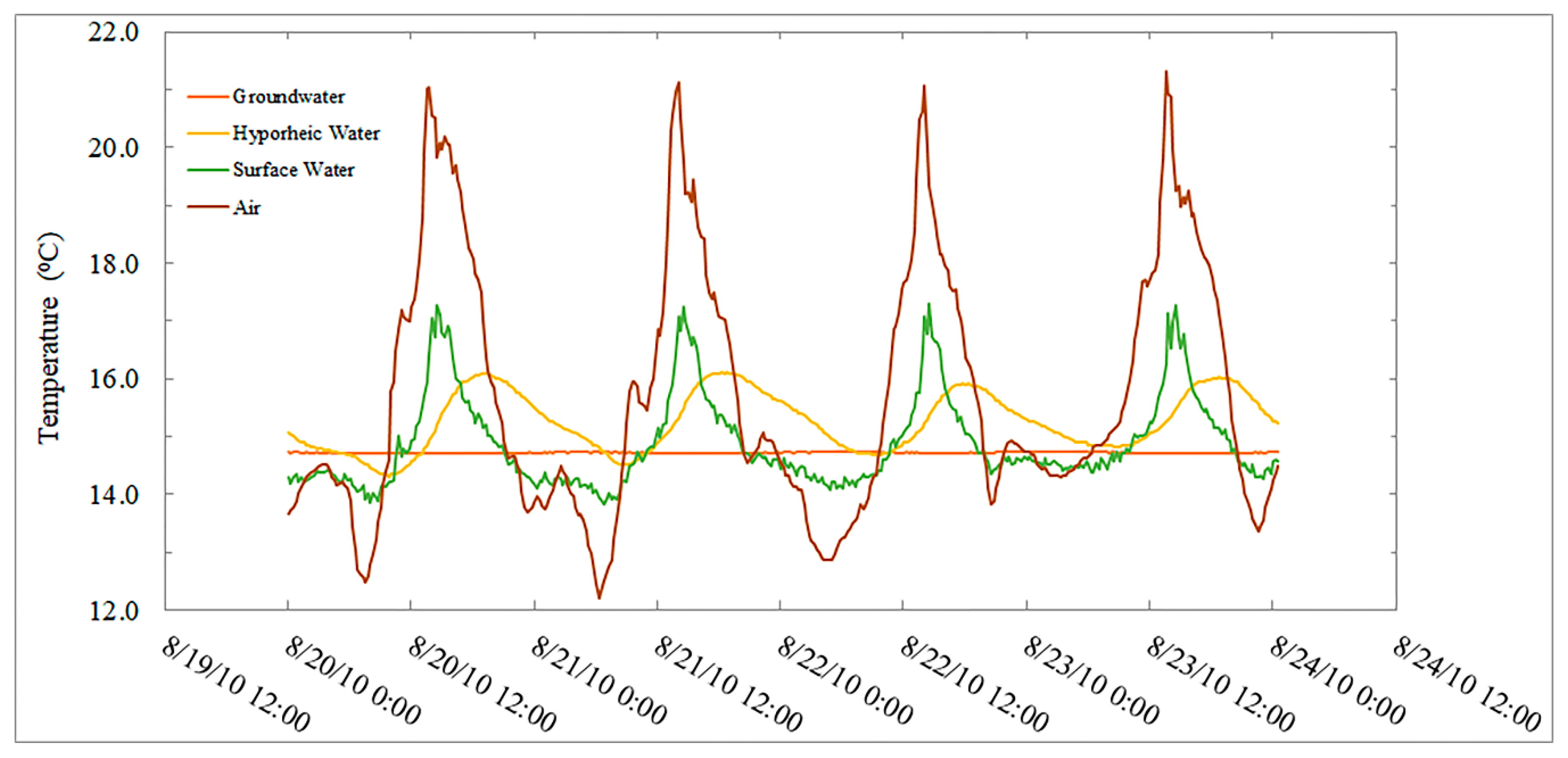
The streamflow and hyporheic exchange rates along the North Fork and main stem reaches were determined from the dye tracer injections (Table 2). Groundwater gains to streamflow were not detected based on no net change in streamflow, excluding tributary inflows, in the study site. The cascade, step-pool, and LWD forced-pool morphology yielded relatively high hyporheic exchange rates of 0.00073 to 0.00053 m3 s−1 m−1. Diurnal fluctuations in hyporheic water temperature were less than surface water temperatures, which in turn were less than air temperatures while groundwater temperatures had negligible diurnal fluctuations (Figure 3).
3.2. Heat Budget Comparisons to Measured Stream Water Temperatures
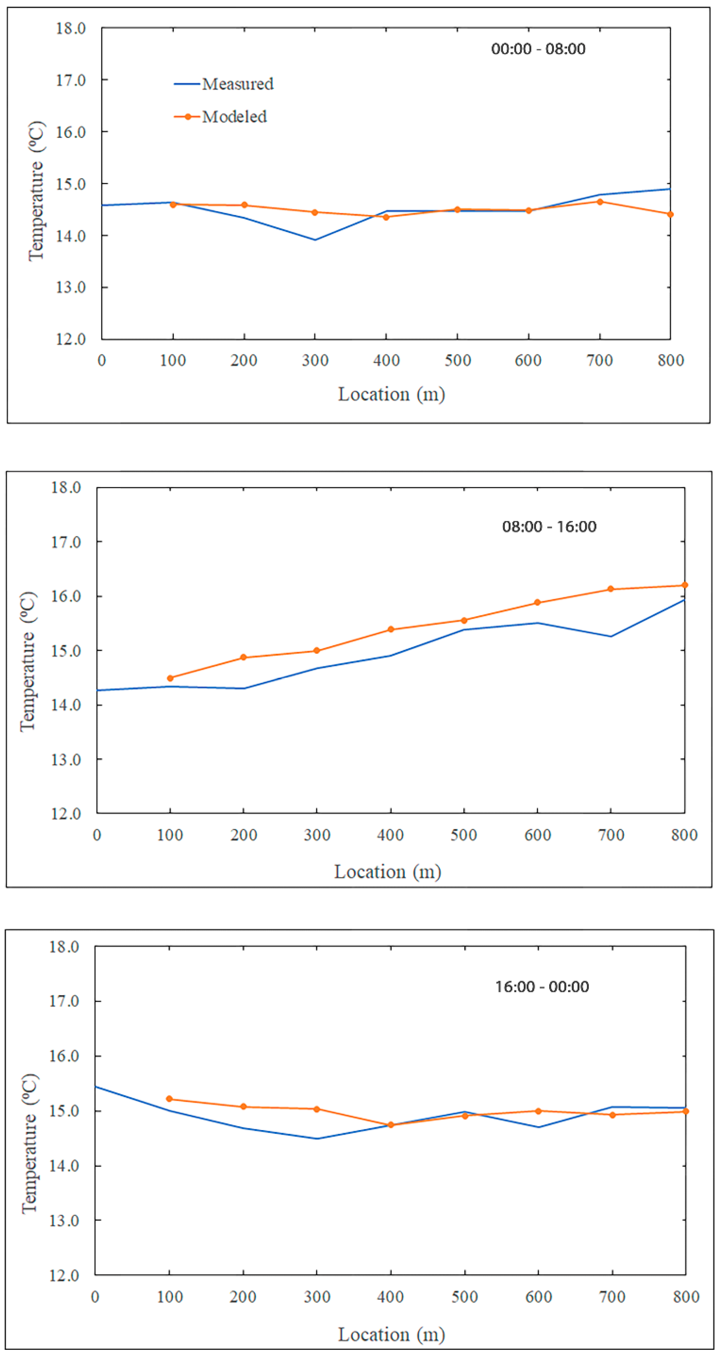
A time step of 1 h (h) and distance step of 100 m, based on average stream residence times determined by dye tracer analysis (Table 2), were used to predict stream water temperature change over the study site. Generally, the stream water temperatures predicted from the Heat Budget model were similar to measured stream water temperatures: root mean square error (RMSE) of 0.1, 0.2 and 0.1 °C for the 100 m, 300 m, and 800 m locations, respectively. The heat-budget-predicted stream water temperatures were calculated by changes in the time interval and distance traveled, known as a Lagrangian frame of reference. A parcel of water would travel 800 m in 8 h in the Little Creek study site, based on average water residence time of 1 h per 100 m (Figure 4). In this approach, differences in heat budget temperature estimates compared to measured temperatures were within 0.5 °C for all three 8 h time periods (Figure 4). However, the heat-budget-predicted stream water temperatures compared to measured temperatures showed as much as a 1 °C error at location 700 m during the 08:00–16:00 time period (Figure 4).
Localized areas of stream heating and cooling are evident for all three 8 hr time periods and were related to correlations with individual heat budget components (Table 3). Hyporheic (Qhyp) and streambed conduction (Qc) heat fluxes had moderate negative correlations (r values −0.614 and −0.583) with downstream water temperature change over the first 100 m (Table 3). From locations 100 m to 300 m, hyporheic (Qhyp) and streambed conduction (Qc) heat fluxes had strong negative correlations (r values of −0.837) while net radiation (Nr) began to exhibit a positive correlation on stream water temperatures, likely due to decreases in stream shading between locations 100 m and 300 m. An additional net warming effect between locations 300 m and 800 m led to warmer daily maximum and average stream water temperatures observed at location 800 m (Figure 2). From 300 m to 800 m, hyporheic flux (Qhyp) and streambed conduction (Qc) had strong negative correlations with temperature change (r values −0.769 and −0.694) while the positive correlation of net radiation (Nr) became stronger (r value of 0.411) (Table 3). Latent heat exchange (Qe) and sensible heat flux (Qh) only had weak correlations with stream water temperatures (−0.261 < r value < 0.271) over all distances observed. The heat fluxes for the midday on the warmest day of the study, 23 August 2014 at 300 m location area are shown for the existing condition and for the 50 and 0 percent shade reduction scenarios (Table 4).
3.3. Stream Water Temperature Change from Shade Reduction
Heat-budget-predicted daily maximum stream water temperature change was averaged over a four-day period for different effective shade scenarios (Table 5). Mean maximum stream water temperature increased by 1.7 to 2.2 °C for the 50% and 0% effective shade scenarios, respectively, at the downstream end of the 300 m treatment reach. Mean maximum stream water temperature at location 800 m, 500 m below the 300 m treatment reach, decreased by 0.2 for the 50% effective shade and increased by 0.2 °C for the 0% effective shade (Table 5). Considering the 0.7 °C measured increase in maximum stream water temperature from locations 300 m to 800 m, when shaded (92% effective shade), the expected outcome following effective shade reduction should include this increase to the already increased maximum stream water temperatures or 2.4 and 2.9 °C, for the 50% and 0% effective shade, respectively. The heat budget results from locations 300 m to 800 m were lower, suggesting a cooling of stream water of 52% and 30% from the expected maximum stream water temperature for the 50% and 0% effective shade scenarios, respectively.
Mean maximum stream water temperature changes predicted by an equation representing only net radiation heating [18] were higher than the heat budget estimates at the 50% and 0% effective shade scenarios from locations 0 to 300 m and 300 m to 800 m. When the influence of hyporheic water exchange was included with the net radiation equation, mean maximum stream water temperature changes were similar to measured temperatures and heat budget estimates, particularly at the 800 m location under current shade conditions (Table 5). The resulting stream water temperatures predicted by these changes are shown (Table 6).
4. Discussion
4.1. Heat Exchange Influences on Stream Water Temperature
Heat budget modeling provided the ability to evaluate temperature impacts downstream from an added heat source, in this case, increased solar radiation from reduction in effective shade. It further provided assessment of the relative associations of individual heat budget components to localized stream heating and cooling. Hyporheic heat exchange (Qhyp) and streambed conduction (Qc) had strong negative correlations (r < −0.700) with temperature change on Little Creek (Table 3). Water in the hyporheic zone had longer hydraulic residence time and contact with the streambed where the two heat budget components work in tandem [28,38]. Observed hyporheic exchange rates of 0.00053 to 0.00073 m3 s−1 m−1 were relatively high compared to streamflow of 0.0027 and 0.0053 m3 s−1. We estimate the amount of hyporheic exchange to be approximately 70% of streamflow, calculated by 1 minus the ratio of hyporheic exchange (m3 s−1 m−1) and streamflow (m3 s−1) times 1 m. The high amount of hyporheic exchange can partially be attributed to the step-pool, cascade, and LWD forced-pool morphology, which have been found to promote concentrated areas of downwelling and subsurface water mixing, particularly in riffles downstream of pools [23,24,38,39].
The percent reduction in downstream water temperature change predicted by the heat budget model 500 m below the effective shade scenarios of 50% and 0% were estimated to be 52% and 30%, respectively. The percent reduction in downstream water temperature change following effective shade reduction, predicted by the combined net radiation and hyporheic mixing equations, were estimated to be 77% and 70%, respectively. Differences in cooling between the heat budget model and mixing model results were likely due to the heat budget model’s consideration of additional heat transfers from streambed conduction, sensible heat and latent heat, which are not accounted for in the mixing model.
A study in coastal Oregon showed that stream water temperature changes were reduced by an average of 56% within the first 300 m of entering a well-shaded stream reach and could be predicted by Newton’s law of cooling [19]. Newton’s law of cooling suggests that convective heat fluxes from the surrounding environment play a significant role in the reduction of stream water temperatures following stream heating. The heat budget components of latent heat exchange and sensible heat exchange for Little Creek, considered convective heat transfers [19], had weak correlations with stream water temperatures (−0.26 < r < 0.27) (Table 3). Additionally, sensible heat flux did not have statistically significant correlations with stream water temperatures (p values >0.05) (Table 3). The percent reduction in maximum stream water temperatures is similar to the range of cooling calculated from Newton’s law of cooling in streams of coastal Oregon [19]. However, in the case of Little Creek, advective heat transfers due to hyporheic exchange and streambed conduction were the primary influence on downstream cooling. The streams in coastal Oregon had gradients between 0.01 and 0.1 m/m and cross-sections areas of 0.1 to10.0 m2, suggesting higher streamflow during low-flow conditions than Little Creek. The larger surface cross-section for the coastal Oregon streams might have promoted greater interaction with above-ground convective heat budget processes than Little Creek.
4.2. Hydrologic Influence on Downstream Water Temperature Following Shade Reduction
Net radiation heat flux alone produces greater increases in daily maximum stream water temperatures compared to the measured, heat budget, and the combined net radiation and hyporheic mixing equation estimates of stream water temperatures (Table 4). For the 0% effective shade scenario, the net radiation equation predicted increases in maximum stream water temperatures of 5.6 and 2.8 °C greater than the heat budget model estimates from locations 300 m to 800 m, respectively. In contrast, maximum stream water temperature changes were similar to the heat budget model predictions when a mixing equation using hyporheic water was included with the net radiation equation, with the exception of the 0% effective shade scenario (Table 5). The net radiation and hyporheic water mixing equation predicted a 1 °C greater increase in maximum stream water temperature than the heat budget from locations 0 to 300 m under the 0% effective shade scenario.
Although care must be taken in comparing treatment effects between studies due to climate and streamflow differences, other studies found similar and higher maximum stream water temperature increases due to shade reduction. Moore et al. [24] observed an approximately 5 °C increase in daily maximum temperatures downstream of a clear-cut harvest in a headwater stream in coastal British Columbia. Heat budget modeling in the Moore et al. study [24] indicated that hyporheic exchange promoted localized daytime cooling effects. The incoming solar radiation and hyporheic heat fluxes for the British Columbia stream at midday were reported to be approximately 900 W/m2 and −175 W/m2, respectively [24]. Little Creek midday solar radiation and hyporheic heat fluxes were similar at 870 W/m2 and −113 W/m2, respectively. However, the Little Creek stream water temperatures were not predicted to increase as much. The heat budget model and net radiation model with mixing of hyporheic water had similar results at 800 m at Little Creek (Table 6). This demonstrates the role advective heat transfers from hyporheic water had in stream cooling and is indicative of the negative heat fluxes for hyporheic exchange. Additionally, the net radiation equation closely predicted the maximum stream water temperature for current conditions at 300 m and 800 m. The net radiation equation modified the incoming solar radiation by the portion of streamflow estimated to be associated with hyporheic exchange (MF). This suggests that the hyporheic exchange in Little Creek also affected stream water temperatures by the reduction in amount of surface water exposure to solar radiation heat fluxes, not quantified in the heat budget values.
In a headwater stream in the western Cascades of Oregon, following timber harvest, daily maximum stream water temperature increased by 7 °C [28]. This stream was similar in size to Little Creek but with bedrock substrate. Streambed conduction from the bedrock channel, with no hyporheic exchange, was reported to be an influential factor in this large stream water temperature increase. In the bedrock channel, midday heat flux for net radiation and streambed conduction were 860 W/m2 and 33 W/m2, respectively, with no hyporheic heat flux. In the bedrock channel streambed, conduction did lower with shade [28]. In Little Creek, net radiation and streambed conduction heat fluxes were 870 W/m2 and −38.5 W/m2, respectively, for the 0% effective shade scenario. The difference in streambed conduction heat fluxes illustrates that the streambed can create a positive heat exchange when subjected to direct solar radiation. Other studies have shown significant influence from streambed conduction particularly in shallow streams [38]. Our model did not incorporate an increase in heat from solar radiation to the streambed which could represent a potential underestimate of the maximum stream water temperature change predicted.
Increase in streamflow by groundwater inputs was not detected at the Little Creek study site, however, it must be noted that the potential for increases in groundwater inflows following near stream vegetation removal can be significant [22,40,41,42]. Wick [43] found that thinning along a 330 m stream reach in northern California, which reduced the canopy over the stream by 5 to 20%, resulted in higher measured streamflow post-thinning despite lower observed annual and spring precipitation. Bond et al. [17] demonstrated through heat budget modeling that increased riparian shading along the Klamath River reduced streamflow. However, the additional riparian vegetation could potentially mitigate increases in mean air temperature and subsequent stream water temperature increases even with reductions in streamflow.
4.3. Evaluation of Downstream Stream Water Temperature Risks for Regulatory Purposes
The results of this study suggest that when advective heat transfers are occurring in streams with step-pool, cascade, and LWD forced-pool morphology, some shade reduction can occur and not cause adverse biological impacts. For example, weekly average maximum stream temperature thresholds for steelhead trout are listed as <17 °C (good) and 17–19 °C (marginal) [10]. Identification of areas with high rates of hyporheic exchange, where advective heat transfer occurs, could provide land managers greater flexibility for management activities that promote improved riparian conditions with low, short-term stream water temperature impacts. Post-treatment temperatures are predicted to be elevated at a distance of 500 m downstream of the hypothetical 300 m treatment reach. This increased heat, as it is transferred downstream toward lower gradient habitat, would need to be considered. Additional reductions in stream water temperature will likely occur if the stream continues to flow through a well-shaded environment or is subject to nighttime cooling, provided similar gradient and channel morphology exists. This could justify some effective shade reduction even when more stringent regulatory targets are required downstream.
The heat budget model is not independent of actual stream water temperature. In other words, the heat budget calculations for Little Creek would have to be repeated at other locations, albeit with the large data requirements, if this approach was to be used in a regulatory evaluation. Conversely, the net radiation model [18] can easily be calculated with lower data requirements than the heat budget approach. However, the rate of hyporheic exchange would need to be determined or estimated. An alternative to this approach would be to measure stream water temperature, hyporheic water temperature, and streamflow longitudinally and from any tributaries to the stream in question. A heat transport model could be fitted to the streamflow, hyporheic temperatures, and stream water temperature measurements. In this way, it could be discovered if advective transfers are influencing stream water temperatures and the magnitude of that effect. The heat transport model could then be calibrated to evaluate effective shade reduction impacts on stream water temperatures.
5. Conclusions
Stream water temperature, climate, and dye tracer measurements, combined with heat budget modeling, provided insight for a headwater stream with cascade, step-pool, and LWD forced-pool morphology. Changes to net radiation from reduction in forest canopy was determined to have the most influential impact on stream water temperatures (Pearson correlation coefficient 0.411; p value <0.001). Advective heat transfer from hyporheic exchange, combined with subsequent streambed conduction, were highly correlated to stream water temperatures along Little Creek (Pearson correlation coefficients −0.694 and −0.769; p values <0.001). These advective heat transfers were found to influence the magnitude and distribution of stream water temperatures and helped explain the spatial variability of observed stream water temperatures.
Both a heat budget model and a net radiation model mixed with hyporheic water were found to provide reasonable estimates for measured stream water temperatures. Both provided similar downstream predictions, an increase of 2.4 °C and 2.3 °C, respectively, when perturbed by reduction in effective shade, providing a validation of the influence of hyporheic advection on downstream cooling. This additionally demonstrated that hyporheic exchange affected stream water temperatures by the reduction in amount of surface exposure water has to solar radiation heat fluxes. Even with the limitations and uncertainty of a modeling approach, the results suggest for that streams with similar physical characteristics as Little Creek, effective shade reduction can be utilized without impacting water-temperature-sensitive species. More research is needed to attempt to develop simple field methods to determine the risks to downstream stream water temperature increases when stream shade is removed.
Author Contributions
Conceptualization, S.C.; Methodology, S.C. and L.J.; Formal Analysis, L.J. and S.C.; Investigation, L.J.; Data Curation, S.C. and L.J.; Writing-Original Draft Preparation, L.J. and S.C.; Writing-Review & Editing, S.C and L.J.; Visualization, L.J.; Supervision, S.C.; Project Administration, S.C.; Funding Acquisition, S.C.
Funding
This research was funded by grants from the California State Universities Agriculture Research Initiative grant number ARI-14-03-01 and McIntire Stennis funds grant number 14-210.
Acknowledgments
Cal Poly’s Swanton Pacific Ranch supported this research by providing access to the study site and assistance from undergraduate student interns in field data collection efforts. The Center for Transformative Environmental Monitoring Programs (CTEMP, based at University of Nevada, Reno) provided an affordable lease and support for the DTS equipment.
Conflicts of Interest
The authors declare no conflict of interest.
References
- Johnson, S.L.; Jones, J.A. Stream temperature responses to forest harvest and debris flows in western Cascades, Oregon. Can. J Fish. Aquat. Sci. 2000, 57, 30–39. [Google Scholar] [CrossRef]
- Beschta, R.; Bilby, R.; Brown, G.; Holtby, L.; Hofstra, T. Stream Temperature and Aquatic Habitat: Fisheries and Forestry Interactions. In Streamside Management: Forestry and Fishery Interactions; Salo, E.O., Cundy, T.W., Eds.; University of Washington: Seattle, WA, USA, 1987; pp. 191–232. [Google Scholar]
- Brown, G.W.; Krygier, J.T. Effects of clear-cutting on stream temperature. Water Resour. Res. 1970, 6, 1133–1139. [Google Scholar] [CrossRef]
- Hairston-Strang, A.; Adams, P.; Ice, G. The Oregon Forest Practices Act and forest research. In Hydrological and Biological Responses to Forest Practices; Stednick, J., Ed.; Springer: Berlin, Germany, 2008; pp. 95–114. [Google Scholar]
- Navarro River Total Maximum Daily Loads for Sediment and Temperature; U.S. Environmental Protection Agency (USEPA): Washington, DC, USA. Available online: http://www.waterboards.ca.gov/northcoast/water_issues/programs/tmdls/navarro_river/110708/navarro.pdf (accessed on 26 October 2018).
- California State Water Resources Control Board (SWRCB) Home Page. Available online: https://www.waterboards.ca.gov/water_issues/programs/water_quality_assessment/#impaired (accessed on 26 October 2018).
- California Forest Practice Rules; California Department of Forestry and Fire Protection (CDF): Sacramento, CA, USA, 2017. Available online: http://calfire.ca.gov/resource_mgt/downloads/2017%20Forest%20Practice%20Rules%20and%20Act.pdf (accessed on 1 June 2015).
- Oregon Department of Forestry (ODF). Oregon Forest Practice Act and Rules; Oregon Department of Forestry (ODF): Salem, OR, USA. Available online: http://www.oregon.gov/ODF/Working/Pages/FPA.aspx (accessed on 26 October 2018).
- Washington Department of Natural Resources (WDNR). Forest Practice Rules and Manual; Washington Department of Natural Resources (WDNR): Olympia, WA, USA. Available online: https://www.dnr.wa.gov/about/boards-and-councils/forest-practices-board/forest-practices-rules-and-board-manual-guidelines (accessed on 26 October 2018).
- California North Coast Regional Water Board (CNCRWB). California Regional Water Quality Control Board, North Coast Region Navarro River Watershed; Technical Support Document for the Total Maximum Daily Load for Sediment and Technical Support Document for the Total Maximum Daily Load for Temperature; California North Coast Regional Water Board (CNCRWB): Santa Rosa, CA, USA, 2000. Available online: http://www.waterboards.ca.gov/northcoast/water_issues/programs/tmdls/navarro_river/navarrotsd.pdf (accessed on 26 October 2018).
- Luce, C.; Staab, B.; Kramer, M.; Wenger, S.; Isaak, D.; McConnell, C. Sensitivity to summer stream temperatures to climate variability in the Pacific Northwest. Water Resour. Res. 2014, 50, 3428–3443. [Google Scholar] [CrossRef]
- Isaak, D.J.; Wollrab, S.; Horan, D.; Chandler, G. Climate change effects on stream and river temperatures across the northwest U.S. from 1980–2009 and implications for salmonid fishes. Clim. Chang. 2012, 113, 499–524. [Google Scholar] [CrossRef]
- Caissie, D. The thermal regime of rivers: A review. Freshw. Biol. 2006, 51, 1389–1406. [Google Scholar] [CrossRef]
- Schwarzenegger, A.; Snow, L.; Walters, D. California’s Forest and Rangeland: 2010 Assessment; California Department of Forestry and Fire Protection (CAL FIRE): Sacramento, CA, USA, 2010. Available online: http://frap.fire.ca.gov/data/assessment2010/pdfs/california_forest_assessment_nov22.pdf (accessed on 1 August 2018).
- California Department of Forestry and Fire Protection (CDF). Anadromous Salmonid Protection Rule Section V. Site-Specific Riparian Management: Section V Guidance; California Department of Forestry and Fire Protection (CDF): Sacramento, CA, USA, 2013. Available online: http://bofdata.fire.ca.gov/board_committees/vtac/vtac_guidance_document_/vtac_guidancedocument_dec21-2012_final.pdf (accessed on 10 September 2018).
- Moore, R.D.; Sutherland, P.; Gomi, T.; Dhakal, A. Thermal regime of a headwater stream within a clear-cut, coastal British Columbia, Canada. Hydrol. Process. 2005, 19, 2591–2608. [Google Scholar] [CrossRef]
- Bond, R.M.; Stubblefield, A.P.; Van Kirk, R.W. Sensitivity of summer stream temperatures to climate variability and riparian reforestation strategies. J. Hydrol. Reg. Stud. 2015, 4, 267–279. [Google Scholar] [CrossRef]
- Brown, G. An Improved Temperature Prediction Model for Small Streams; Oregon State University: Corvallis, OR, USA, 1971; p. 24. [Google Scholar]
- Davis, L.J.; Reiter, M.; Groom, J.D. Modelling temperature change downstream of forest harvest using Newton’s law of cooling. Hydrol. Process. 2016, 30, 959–971. [Google Scholar] [CrossRef]
- Garner, G.; Malcolm, I.A.; Sadler, J.P.; Hannah, D.M. The role of riparian vegetation density, channel orientation and water velocity in determining river temperature dynamics. J. Hydrol. 2017, 553, 471–485. [Google Scholar] [CrossRef]
- Zwieniecki, M.; Newton, M. Influence of streamside cover and stream features on temperature trends in forested streams of western Oregon. West. J. Appl. For. 1999, 14, 106–113. Available online: http://www.scopus.com/inward/record.url?eid=2-s2.00032669081&partnerID=40&md5=078a8d31bf69ef8e88e0eacf284d3fe3 (accessed on 26 October 2018).
- Story, A.; Moore, R.; Macdonald, J. Stream temperatures in two shaded reaches below cutblocks and logging roads: Downstream cooling linked to subsurface hydrology. Can. J. For. Res. 2003, 33, 1383–1396. [Google Scholar] [CrossRef]
- Danehy, R.J.; Colson, C.G.; Parrett, K.B.; Duke, S.D. Patterns and sources of thermal heterogeneity in small mountain streams within a forested setting. For. Ecol. Manag. 2005, 208, 287–302. [Google Scholar] [CrossRef]
- Moore, R.D.; Spittlehouse, D.L.; Story, A. Riparian microclimate and stream temperature response to forest harvesting: A review. J. Am. Water Resour. Assoc. 2006, 7, 813–834. [Google Scholar] [CrossRef]
- Malard, F.; Mangin, A.; Uehlinger, U.; Ward, J.V. Thermal heterogeneity in the hyporheic zone of a glacial floodplain. Can. J. Fish. Aquat. Sci. 2001, 58, 1319–1335. [Google Scholar] [CrossRef]
- Martin, D.; Liquori, M.; Coats, R.; Benda, L.; Ganz, D. Scientific Literature Review of Forest Management Effects on Riparian Functions for Anadromous Salmonids, Chapter 3 Heat Exchange Function; Report prepared by Sound Watershed Consulting for the California State Board of Forestry and Fire Protection; Sound Watershed Consulting: Oakland, CA, USA, 2008; Available online: http://www.soundwatershed.com/uploads/2/3/8/1/2381599/3_heat_exchange_functions.pdf (accessed on 26 October 2018).
- Tonina, D.; Buffington, J.M. Hyporheic exchange in mountain rivers: Mechanics and environmental effects. Geogr Compass. 2009, 3, 1063–1086. [Google Scholar] [CrossRef]
- Johnson, S.L. Factors influencing stream temperatures in small streams: Substrate effects and a shading experiment. Can. J. Fish. Aquat. Sci. 2004, 61, 913–923. Available online: http://www.nrcresearchpress.com/doi/abs/10.1139/f04-040 (accessed on 10 September 2018). [CrossRef]
- Piirto, D.; Thompson, R.; Piper, K. Implementing Uneven-Aged Redwood Management at Cal Poly’s School Forest, an Update. Available online: https://content-calpoly-edu.s3.amazonaws.com/spranch/1/documents/Swanton_NTMP/Piirtoetal1999.pdf (accessed on 23 August 2015).
- North Central Coast Salmon and Steelhead Recovery Plans; National Oceanic Atmospheric Administration (NOAA): Washington, DC, USA. Available online: https://www.westcoast.fisheries.noaa.gov/protected_species/salmon_steelhead/recovery_planning_and_implementation/ (accessed on 26 October 2018).
- Selker, J.S.; Thévenaz, L.; Huwald, H.; Mallet, A.; Luxemburg, W.; Van De Giesen, N.; Stejskal, M.; Zeman, J.; Westhoff, M.; Parlange, M.B. Distributed fiber-optic temperature sensing for hydrologic systems. Water Resour. Res. 2006, 42, W12202. [Google Scholar] [CrossRef]
- Tyler, S.; Selker, J.; Hausner, M.; Hatch, C.; Torgersen, T.; Thodal, C.; Schladow, S. Environmental temperature sensing using Raman spectra DTS fiber-optic methods. Water Resour. Res. 2009, 45, W00D23. [Google Scholar] [CrossRef]
- Hausner, M.B.; Suárez, F.; Glander, K.E.; van de Giesen, N.; Selker, J.S.; Tyler, S.W. Calibrating single-ended fiber-optic Raman spectra distributed temperature sensing data. Sensors 2011, 11, 10859–10879. [Google Scholar] [CrossRef] [PubMed]
- Kilpatrick, F.; Frederick, A.; Cobb, E. Measurement of Discharge Using Tracers Home Page. Available online: water.usgs.gov/software/OTIS/addl/readinglists/tracer_methods.html (accessed on 26 October 2018).
- Runkel, R. One-Dimensional Transport with Inflow and Storage (OTIS): A Solute Transport Model for Streams and Rivers; U.S. Geological Survey: Reston, VA, USA, 1998; p. 73.
- Harvey, J.; Wagner, B.; Bencala, K. Evaluating the reliability of the stream tracer approach to characterize stream-subsurface exchange. Water Resour. Res. 1996, 32, 2441–2451. [Google Scholar] [CrossRef]
- California Irrigation Management Information System (CIMIS). Station: De Laveaga Home Page. Available online: www.cimis.water.ca.gov/WSNReportCriteria.aspx (accessed on 6 January 2016).
- Caissie, D.; Luce, C.H. Quantifying streambed advection and conduction heat fluxes. Water Resour. Res. 2017, 53, 1595–1624. [Google Scholar] [CrossRef]
- Burkholder, B.; Grant, G.; Haggerty, R.; Khangaonkar, T.; Wampler, P. Influence of hyporheic flow and geomorphology on temperature of a large, gravel-bed river, Clackamas River, Oregon, USA. Hydrol. Process. 2008, 22, 941–953. [Google Scholar] [CrossRef]
- Mellina, E.; Moore, R.; Hinch, S.; Stevenson, M.J.; Pearson, G. Stream temperature responses to clearcut logging in British Columbia: The moderating influences of groundwater and headwater lakes. Can. J. Fish. Aquat. Sci. 2002, 59, 1886–1900. [Google Scholar] [CrossRef]
- Sinokrot, B.A.; Stefan, H.G. Stream temperature dynamics: Measurements and modeling. Water Resour. Res. 1993, 29, 2299–2312. [Google Scholar] [CrossRef]
- Surfleet, C.G.; Skaugset, A.E. The effect of timber harvest on summer low flows, hinkle creek, Oregon. West. J. Appl. For. 2013, 28, 13–21. [Google Scholar] [CrossRef]
- Wick, A. Adaptive Management of a Riparian Zone in the Lower Klamath River Basin, Northern California: The Effects of Riparian Harvest on Canopy Closure, Water Temperatures and Baseflow. Master’s Thesis, Humboldt State University, Arcata, CA, USA, July 2016. [Google Scholar]
Figure 1.
Little Creek study site location, Santa Cruz County, CA, USA.

Figure 2.
Minimum, maximum, 25th and 75th percentile, and median observed daily maximum temperatures (°C) per location on Little Creek from 21 to 25 August 2014.
Figure 2.
Minimum, maximum, 25th and 75th percentile, and median observed daily maximum temperatures (°C) per location on Little Creek from 21 to 25 August 2014.

Figure 3.
Observed air, surface, hyporheic and groundwater temperatures on Little Creek at location 390 m from 21 to 25 August 2014. Groundwater temperature was measured at a nearby spring.
Figure 3.
Observed air, surface, hyporheic and groundwater temperatures on Little Creek at location 390 m from 21 to 25 August 2014. Groundwater temperature was measured at a nearby spring.

Figure 4.
Lagrangian plots for Little Creek comparing observed and heat-budget-modeled temperatures for three 8 h time periods on 24 August 2014 as water traveled downstream from locations 0 to 800 m.
Figure 4.
Lagrangian plots for Little Creek comparing observed and heat-budget-modeled temperatures for three 8 h time periods on 24 August 2014 as water traveled downstream from locations 0 to 800 m.


Table 1.
Physical measurements of the Little Creek study site from 21 to 25 August 2014 taken at 25 m intervals along 825 m study reach.
Table 1.
Physical measurements of the Little Creek study site from 21 to 25 August 2014 taken at 25 m intervals along 825 m study reach.
| Dimension | Mean | Standard Error |
|---|---|---|
| Wetted width (m) | 1.48 | 0.63 |
| Water depth (m) | 0.07 | 0.06 |
| Bankfull width (m) | 3.67 | 1.08 |
| Aspect ratio (m/m) | 35 | 45.4 |
| Median streambed particle size (D50) (mm) | 27 | 18 |
| August solar path shading (%) | 92 | 4 |
| Channel slope (m/m) | 0.05 | - |
| Watershed area (ha) | 670 | - |
Table 2.
Streamflow (qs), hyporheic exchange rate (qhyp), residence time (Ts) (hrs/100 m), subsurface cross section area (As) determined from rhodamine dye injection analysis. Stream cross-section is the average of channel measurements (A).
Table 2.
Streamflow (qs), hyporheic exchange rate (qhyp), residence time (Ts) (hrs/100 m), subsurface cross section area (As) determined from rhodamine dye injection analysis. Stream cross-section is the average of channel measurements (A).
| Little Creek Location | Date | qs (m3 s−1) | A (m2) | qhyp (m3 s−1 m−1) | Ts (hrs/100 m) | As (m2) | As/A |
|---|---|---|---|---|---|---|---|
| North Fork | 21 August 2014 | 0.0027 | 0.08 | 0.00073 | 0.9 | 4.54 | 54.8 |
| Main Stem | 25 August 2014 | 0.0057 | 0.14 | 0.00053 | 1.1 | 4.99 | 36.3 |
Table 3.
Little Creek correlation results comparing heat budget components—including net radiation (Nr), streambed conduction (Qc), latent heat exchange (Qe), sensible heat (Qh), and hyporheic flux (Qhyp)—with hourly stream water temperature change. Results include sample size (n), Pearson correlation coefficient (r) and statistical significance (p) per stream reach distance evaluated.
| Distance (Sample Size) | 0–100 m (n = 102) | 100–300 m (n = 102) | 300–800 m (n = 97) | |||
|---|---|---|---|---|---|---|
| Heat Flux | r | p | r | p | r | p |
| Nr | −0.295 | 0.003 | 0.162 | 0.105 | 0.411 | <0.001 |
| Qc | −0.583 | <0.001 | −0.837 | <0.001 | −0.694 | <0.001 |
| Qe | −0.261 | 0.008 | 0.249 | 0.012 | 0.271 | 0.007 |
| Qh | −0.178 | 0.074 | 0.055 | 0.582 | 0.171 | 0.094 |
| Qhyp | −0.614 | <0.001 | −0.837 | <0.001 | −0.769 | <0.001 |
Table 4.
Measured net radiation flux (Nr) for open sky, net radiation heat flux adjusted for 50% effective shade and 92% canopy and the associated estimated heat fluxes of streambed conduction (Qc), latent heat exchange (Qe), sensible heat (Qh) and hyporheic flux (Qhyp) for midday 23 August 2014.
Table 4.
Measured net radiation flux (Nr) for open sky, net radiation heat flux adjusted for 50% effective shade and 92% canopy and the associated estimated heat fluxes of streambed conduction (Qc), latent heat exchange (Qe), sensible heat (Qh) and hyporheic flux (Qhyp) for midday 23 August 2014.
| Effective Shade Scenario | Nr (W m−2) | Qc (W m−2) | Qe (W m−2) | Qh (W m−2) | Qhyp (W m−2) |
|---|---|---|---|---|---|
| 92% | 53.5 | 8.5 | 0.12 | 8.9 | 19.6 |
| 50% | 446.0 | −12.9 | −0.01 | −1.3 | −40.5 |
| 0% | 870.0 | −38.5 | −0.1 | −25.2 | −113.8 |
Table 5.
Average change in maximum stream water temperatures for current condition of 92% effective shade and predicted conditions of 50% and 0% effective shade from locations 0 to 300 m and 300 m to 800 m on Little Creek.
Table 5.
Average change in maximum stream water temperatures for current condition of 92% effective shade and predicted conditions of 50% and 0% effective shade from locations 0 to 300 m and 300 m to 800 m on Little Creek.
| Location and Effective Shading Scenario | Measured (°C) | Net Radiation Equation (°C) | Heat Budget Model (°C) | Net Radiation Equation Mixed with Hyporheic (°C) |
|---|---|---|---|---|
| 300 m | ||||
| 92% | 0.2 | 0.4 | 0.1 | 0.4 |
| 50% | - | 2.8 | 1.7 | 1.6 |
| 0% | - | 5.6 | 2.2 | 3.2 |
| 800 m | ||||
| 92% | 0.9 | 0.7 | 0.6 | 0.6 |
| 50% | - | 3.5 | 1.5 | 1.3 |
| 0% | - | 6.3 | 2.4 | 2.3 |
Table 6.
Mean maximum stream water temperatures predicted for varying locations and shade scenarios.
Table 6.
Mean maximum stream water temperatures predicted for varying locations and shade scenarios.
| Location and Shading Scenario | Measured (°C) | Net Radiation Equation (°C) | Heat Budget Model (°C) | Net Radiation Equation Mixed with Hyporheic (°C) |
|---|---|---|---|---|
| 300 m | ||||
| 92% | 15.5 | 15.7 | 15.4 | 15.5 |
| 50% | - | 18.1 | 17.0 | 16.9 |
| 0% | - | 20.9 | 17.5 | 18.5 |
| 800 m | ||||
| 92% | 16.2 | 16.0 | 15.9 | 15.9 |
| 50% | - | 18.8 | 16.8 | 16.6 |
| 0% | - | 21.7 | 17.7 | 17.5 |
© 2018 by the authors. Licensee MDPI, Basel, Switzerland. This article is an open access article distributed under the terms and conditions of the Creative Commons Attribution (CC BY) license (http://creativecommons.org/licenses/by/4.0/).
Share and Cite
MDPI and ACS Style
Surfleet, C.; Louen, J. The Influence of Hyporheic Exchange on Water Temperatures in a Headwater Stream. Water 2018, 10, 1615. https://doi.org/10.3390/w10111615
AMA Style
Surfleet C, Louen J. The Influence of Hyporheic Exchange on Water Temperatures in a Headwater Stream. Water. 2018; 10(11):1615. https://doi.org/10.3390/w10111615
Chicago/Turabian StyleSurfleet, Christopher, and Justin Louen. 2018. "The Influence of Hyporheic Exchange on Water Temperatures in a Headwater Stream" Water 10, no. 11: 1615. https://doi.org/10.3390/w10111615
Note that from the first issue of 2016, this journal uses article numbers instead of page numbers. See further details here.