Article

Quantifying Urban Bioswale Nitrogen Cycling in the Soil, Gas, and Plant Phases

1
Department of Civil Engineering and Engineering Mechanics, Columbia University, 500 West 120th Street, 610 Mudd, New York, NY 10027, USA
2
Department of Earth and Environmental Engineering, Columbia University, 500 West 120th Street, 918 Mudd, New York, NY 10027, USA
3
Department of Ecology, Evolution, and Environmental Biology, Columbia University, 1200 Amsterdam Avenue, 10th Floor Schermerhorn Ext, New York, NY 10027, USA
4
Department of Environmental Science, Barnard College, 3009 Broadway, 404 Altschul Hall, New York, NY 10027, USA
5
Department of Biology, University of Oregon, 1210 University of Oregon, 77 Klamath Hall, Eugene, OR 97403, USA
6
Lamont-Doherty Earth Observatory, Columbia University, 61 Route 9W, Palisades, NY 10964, USA
*
Author to whom correspondence should be addressed.
Water 2018, 10(11), 1627; https://doi.org/10.3390/w10111627
Submission received: 22 September 2018 / Revised: 26 October 2018 / Accepted: 6 November 2018 / Published: 12 November 2018
(This article belongs to the Special Issue Plant and Microbial Processes in Stormwater Treatment Systems)

Abstract

:
Bioswales are a common feature of urban green infrastructure plans for stormwater management. Despite this fact, the nitrogen (N) cycle in bioswales remains poorly quantified, especially during dry weather in the soil, gas, and plant phases. To quantify the nitrogen cycle across seven bioswale sites located in the Bronx, New York City, we measured rates of ammonium and nitrate production in bioswale soils. We also measured soil nitrous oxide gas emissions and plant foliar nitrogen. We found that all mineralized nitrogen underwent nitrification, indicating that the soils were nitrogen-rich, particularly during summer months when nitrogen cycling rates increase, as indicated by higher levels of ammonium in the soil. In comparison to mineralization (0 to 110 g N m−2 y−1), the amounts of nitrogen uptake by the plants (0 to 5 g N m−2 y−1) and of nitrogen in gas emissions from the soils (1 to 10 g N m−2 y−1) were low, although nitrous oxide gas emissions increased in the summer. The bioswales’ greatest influx of nitrogen was via stormwater (84 to 591 g N m−2 y−1). These findings indicate that bioswale plants receive overabundant nitrogen from stormwater runoff. However, soils currently used for bioswales contain organic matter contributing to the urban nitrogen load. Thus, bioswale designs should use less nitrogen rich soils and minimize fertilization for lower nitrogen runoff.

Graphical Abstract

1. Introduction

Nitrogen (N) is considered the most problematic pollutant for U.S. coastal waters, having degraded the marine ecosystems, fish production, and recreation of two-thirds of the U.S. coastline [1]. Due to fossil fuel combustion from power plants and vehicles, 47% more nitrogen accumulates on impervious surfaces in urban compared to nonurban areas [2]. Bioswales, which are a common feature of many cities’ green infrastructure (GI) plans, are vegetated structures designed to reduce water pollution by absorbing stormwater runoff from impervious surfaces [3]. However, recent studies have demonstrated that these GI types can contribute to nitrogen pollution [4,5,6,7]. During wet weather conditions, high concentrations of nitrogen enter bioswales via stormwater influent, and potentially exit via surface overflow and/or subsurface infiltration [8,9,10,11]. In dry weather conditions, the nitrogen source comes from soil mineralization, a commonly used index of soil nitrogen availability [12,13,14], which describes the rate that soil microbes decompose long-term stores of organic nitrogen (org–N) into ammonium (NH4+) (Figure 1). Mineralization processes occur in all soils. In well-drained soil environments, nitrifying microbes then further transform this ammonium to nitrate (NO3), the most common drinking water pollutant [15] and a highly mobile anion that readily leaches out of soils [10,16]. Bioswales are most frequently made with fast-draining soils that are primarily aerobic, creating a dry environment hospitable to nitrifying microbes, and thus have high levels of nitrification [5,10,17,18]. Brown et al. [19], Lucas and Greenway [20], and McPhillips et al. [21] suggest that excess mineralization and nitrification account for why bioswales have been found to leach nitrate, which can be quickly flushed out following rain events [4,6,10]. Surprisingly, neither mineralization nor nitrification rates have been well quantified in bioswales.
The measurement of mineralization and nitrification rates in bioswale soils can help quantify the rate at which soils release nitrogen pollution via the conversion of nitrogen from organic to inorganic forms, which are more readily washed out from bioswale soils. In addition, the proportion of mineralized nitrogen that undergoes nitrification can also be used to indicate the concentration of nitrogen species in soils. In nitrogen-rich environments, nitrogen accumulates as nitrate rather than ammonium because nitrifying microbes thrive in such environments. Conversely, when nitrogen is scarce, nitrifying microbes compete poorly for ammonium against plants and heterotrophic microbes, limiting the proportion of nitrogen that accumulates as nitrate [13,22].
Similar to mineralization and nitrification rates, the emission rate of microbially-mediated nitrogen gas (including dinitrogen gas (N2), nitrous oxide (N2O), and nitric oxide (NO)) (Figure 1), can also reflect the nitrogen level in the soil, as emissions increase when the microbes have a greater nitrogen supply [23,24]. McPhillips et al. [25] found roadside ditches to be hotspots for nitrogen emissions due to elevated nitrogen influxes from stormwater runoff. Increased concentrations of nitrogen species from fertilization [25,26,27] and nitrogen deposition [23] are also positively associated with increased nitrogen gas emissions. In fact, nitrous oxide emissions from irrigated urban lawns in California increased from 7.2 μg N m−2 h−1 [28] to 720 μg N m−2 h−1 [29] after the application of fertilizers.
Another indication that bioswale soils might be too nitrogen-rich is when sources of nitrogen (stormwater influent and soil mineralization) exceed plant requirements, after accounting for losses from gas emissions. While ornamental landscapes and trees in urban areas require about 5 to 20 g N m−2 y−1 in fertilizer [30], bioswales might not require fertilization because nitrogen inputs through stormwater inflows already contain significant nitrogen loads [21]. The creation of a comprehensive nitrogen mass balance for urban bioswales would allow comparison of nitrogen levels in plant foliage to nitrogen inputs from stormwater and mineralization, and thus help determine whether bioswale soils are at proper nitrogen levels.
Better quantification of nitrogen cycling in bioswales is the first step toward improving the design and management of these GI installations in order to minimize their nitrogen export [5,31]. In particular, research that examines the distinctions between mineralization, gas emissions, and plant uptake is greatly needed [5,12,32,33]. This study aimed to meet this need by measuring the levels of nitrogen in soil, gas, and plant forms within seven bioswales located in New York City (NYC) over a period spanning from June 2015 to October 2016. The specific objectives of the study were to: (1) quantify spatiotemporal variability of soil mineralization and nitrification across the study sites, (2) measure nitrogen gas emission rates, (3) estimate maximum nitrogen uptake rates by the vegetation, and (4) use the results to construct an overall nitrogen mass balance for a bioswale. The results suggest that bioswale soils should contain greater C:N ratios from the outset and be maintained without additional fertilizers.

2. Materials and Methods
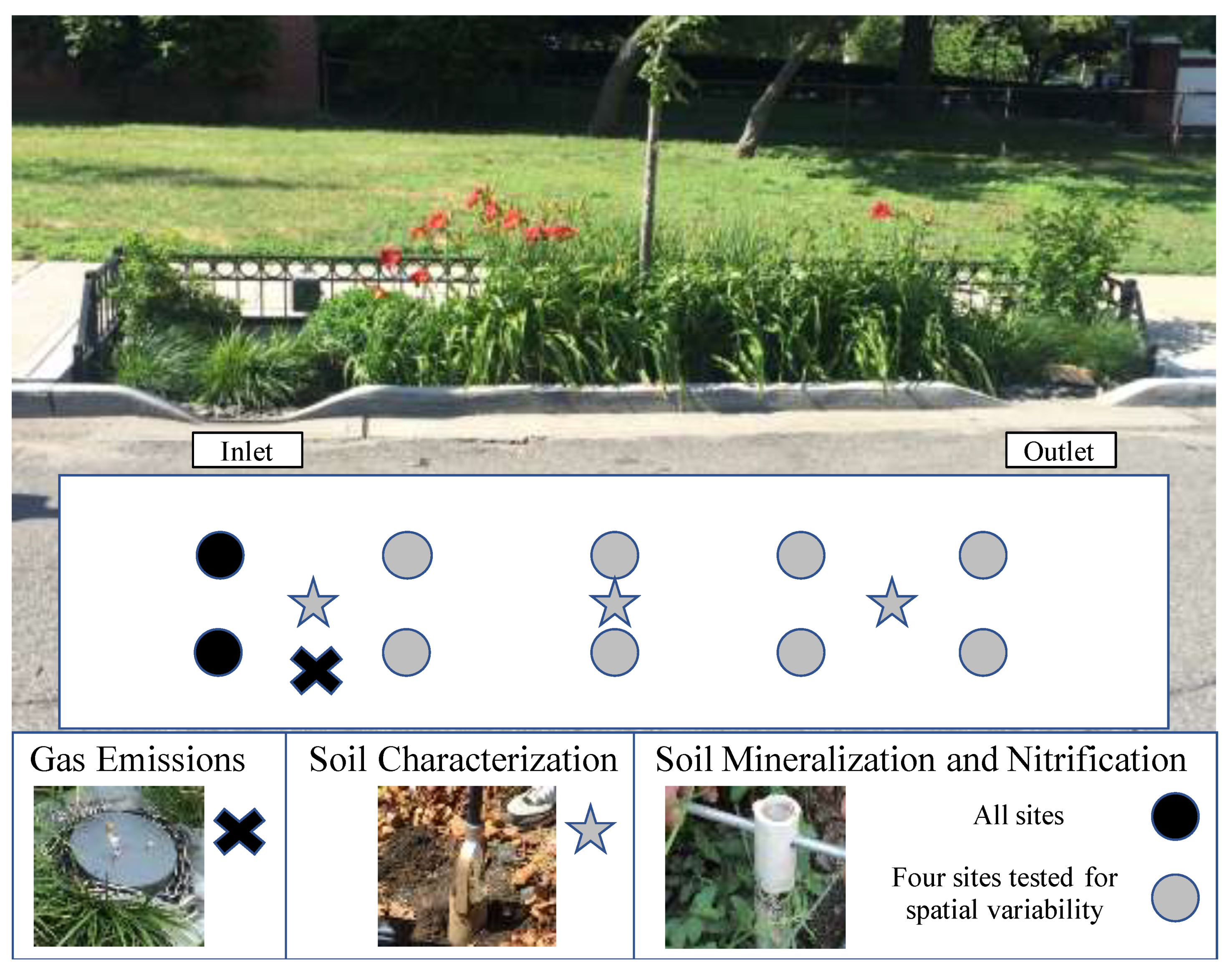
2.1. Bioswale Sites

The seven target bioswales were constructed between April 2013 and April 2014 in the Bronx, NYC, at 40°49′ N, 73°52′ W (Table 1). The total area of the bioswales varied from 7 m2 to 115 m2. Each bioswale contained a 61-cm layer of engineered sandy loam soil. The soil specification used to construct the bioswales is included in the supplemental information. Below the soil lay another 61-cm layer made up of 5-cm-diameter crushed stone. This stone drainage layer was wrapped on all sides with a geotextile filter fabric to separate the stone from the soil without restricting water movement. The soil surface was topped with 7 cm of bark chip mulch, and the bioswales were planted with both native and ornamental plant species including trees, shrubs, grasses, and herbaceous perennials, as detailed in Section 2.4. Stormwater influent entered into the bioswales through curb cut inlets. The bioswales were designed for infiltration and did not contain underdrains. Stormwater that did not infiltrate overflowed through curb cut outlets. Four of the smaller bioswales were termed “right-of-way bioswales” (ROWBs) because they were located in the sidewalk, while the remaining three bioswales, termed “stormwater greenstreets” (SGSs), were larger and extended into the street. Shetty contains a full description of the target bioswale sites [34].
Soil characterization and soil mineralization and nitrification measurements were conducted at all seven sites, with four of the seven sites undergoing more intensive sampling to evaluate spatial variability in soil mineralization and nitrification (Table 1). Soil gas emissions were sampled at one ROWB and one SGS to detect if the size of the sampling site affected results. Plant foliar nitrogen was sampled at the four ROWB sites only, as the SGS sites contained too great a variety of plant species for comparison.
As described in Section 2.2 and Section 2.3, soil mineralization and nitrification and gas emissions measurements were conducted within one meter of each site’s inlet, whereas soil characterization and spatial variability measurements were conducted at regular intervals from the inlet to the outlet (Figure 2). All plants were sampled throughout each site.

2.2. Soil

2.2.1. Soil Characterization

On 30 June 2016, two composite soil samples were taken from each of the seven sites using a circular 7.6-cm-diameter barrel auger [35]. The samples were submitted to the Soil Testing Laboratory at Rutgers University and analyzed for soil texture, organic matter, total carbon, and total nitrogen. The two composite samples consisted of a shallow sample taken from a depth from 7.6 cm to 22.9 cm, and a deeper sample from 30.5 cm to 45.7 cm depth. Each composite was comprised of three subsamples spatially distributed across the site, one located at the inlet to the bioswale, one in the middle of the bioswale, and one near the outlet of the bioswale (Figure 2). The three subsamples were added to the same polyethylene Ziploc bag and homogenized through kneading the bag by hand to create each composite sample.

2.2.2. Soil Mineralization and Nitrification

Soil mineralization and nitrification were analyzed with an intact soil core, a standard method for measuring soil mineralization [36,37]. Cores were housed in two 25.4-mm-inner diameter polyvinyl chloride pipes, each 50.8 cm long, that were sharpened at the bottom to minimize soil disturbance during insertion. These pipes were cut in half lengthwise and duct-taped back together so that they could be opened following retrieval. They were pushed into the soil leaving 5 cm above ground. Each core housing had a pre-cut 1-cm hole at the top for a rebar handle that could be used to pull the core out (Figure 2).
Soil cores were sampled in pairs at each bioswale. The cores were taken within one meter of the bioswale inlet, and 15 cm apart from each other. To test initial ammonium and nitrate levels, the first core was removed immediately, while the other core was left in the ground at the site for a seven-day field incubation period. Neither the initial nor incubated core was consistently in front of the other or closer to the inlet. A photograph was taken to ensure that the same locations would not be sampled on subsequent visits. The hole left after removing each core was backfilled with bioswale soil to restore the site.
Following removal, the duct tape on each core was cut, the pipe was opened and the soil core length measured. The samples from the top and bottom half of the core were then homogenized in separate polyethylene Ziploc bags through kneading the bags by hand. In the field, 5 g of soil sample was added to 50-mL vials that were pre-filled with 30 mL of a 2 M KCl solution; the salts in this solution displace ammonium and nitrate from the soil, allowing quantification of nitrogen levels in the soil via measurement of solution concentration levels. Vials were brought back to the Heck Laboratory located at Barnard College, NYC and shaken at 150 rpm for one hour to allow ammonium and nitrate to dissolve into the solution. Following this, vials were then centrifuged at 4000 rpm for four minutes to filter out the soil using Millex-SV Durapore polyvinylidene fluoride (PVDF) filters (0.22 µm pore size); the resultant solution was then frozen within 6 hours of sampling. To calculate the mass of dry soil used in the 5 g sample, soil moisture was also measured using a gravimetric method [38].
One pair of soil cores was sampled and analyzed at the seven bioswales monthly from June 2015 to August 2016, with the exception of January and February 2016 which were not sampled due to frozen soils. This resulted in the measurement of soil nitrogen content on 26 dates, and the calculation of mineralization and nitrification rates for 13 incubation periods. Within-site spatial variability of soil mineralization and nitrification was measured at four of the seven sites in October and November 2015 (Table 1). The spatial variability test included five pairs of soil cores rather than just one, with each pair evenly spread down the length of the bioswale from the stormwater inlet to the outlet (Figure 2). Ammonium was analyzed by a fluorometric method [39] and nitrate analyzed by ion chromatography [40]. Net mineralization and net nitrification were calculated with the following equation:
Net   Mineralization   and   Net   Nitrification   ( μ g   N   d 1   g 1   dry   soil ) = C i + t C i t
where C represents the concentration of NO3 + NH4+ when calculating net mineralization, C represents the concentration of NO3 only when calculating net nitrification, and t = 7 days. C i refers to concentrations from the immediately sampled soil cores and C i + t refers to concentrations from the soil cores in place for seven days at a site.

2.3. Soil Gas Emissions

Soil gas emissions were sampled at two of the seven sites with a static chamber method, which is the most common method for analysis of N2O fluxes [26,41]. A polyvinyl chloride (PVC) cap soil gas chamber was used, 7 cm in height and 20 cm in diameter, with three Swagelok 3 mm tube compression fittings drilled into the top of the chamber (Figure 2). Two fittings were attached to septa to allow for syringe withdrawal of gas from the chamber, while the third was fixed with a 1.2-m-long, 3-mm-diameter coiled stainless steel tube in order to equalize pressure but prevent significant diffusion of gas out of the chamber. Polyethylene plastic sheeting with a thickness of 4 mm tightly wrapped the chamber and a heavy chain was placed on top of the sheeting to create a seal with the uneven soil. The gas concentration in the chamber was sampled over time, and translated into a flux rate. Gas samples with 15 mL of headspace were taken at 2, 5, 10, and 15 min intervals using a 30-mL syringe and stored in over-pressurized pre-evacuated 10 mL vials.
Gas samples were analyzed for nitrous oxide using a SRI 8610C gas chromatograph (SRI Instruments, Torrance, CA, USA). For each test day and site, soil gas emission was calculated by determining a linear slope of concentration of the four time points [25,42] while considering the footprint and volume of the chamber and the density of air.
Gas fluxes were measured 16 times at two bioswales on eight dates between 15 June 2015 and 21 September 2016. All measurements were conducted during the summer and fall seasons, with the exception of 15 June 2015, which was included with summer samples for statistical analysis. During the sampling dates, the temperature ranged from 8.4 °C to 26.9 °C and the total rain depth over the previous three days before sampling ranged from 0 to 56.1 mm. All measurements were conducted within one meter of the inlets of each site, an area that may have increased soil gas emissions compared to the rest of the site due to greater nitrogen inputs [24].

2.4. Plant Uptake

We measured the level of nitrogen in samples of tissue from ten leaves per plant species, collected among the different plant species present at four different sites (Table 1). The vegetation in the four sampled bioswales was planted such that there were discrete patches covered by each species. We also measured the spatial extent of each plant species by measuring the area covered by each distinct patch for a given species. We selected leaf area indices from published literature, and summed data from all plant patches to estimate total nitrogen content in aboveground foliage.
We sampled 10 leaves collected across the different patches of each plant species at each bioswale on 5 October 2016. On this date, ROWB 9A and ROWB 9B both contained Hemerocallis ‘Lady Florence’, Liriope muscari, Panicum virgatum, Pennisetum alopecuroides, Quercus palustris, Rosa ‘Radrazz’ Knockout, and Symphyotrichum novae-angliae, ROWB 26B contained Amelanchier canadensis, Aronia melanocarpa, Nepeta x faassennii ‘Walker’s Low’, Panicum virgatum, and Spiraea tomentosa; and ROWB 23 contained Aronia melanocarpa, Echinacea purpurea, Eupatorium sp., Nepeta x faassennii ‘Walker’s Low’, and Panicum virgatum. Each collected leaf was photographed in the field immediately after collection with a 7.62 cm × 12.7 cm card for determining scale. Using ImageJ, the perimeter of each leaf was traced to calculate the area. After air drying in the laboratory, all leaves were massed, crushed, ground, and analyzed for carbon and nitrogen using a FlashEA® 1112 Carbon and Nitrogen analyzer (Thermo Scientific, Waltham, MA, USA). We quantified carbon and nitrogen ratios (C:N), nitrogen per unit mass, nitrogen per unit area, and nitrogen per leaf. For statistical analysis, plant species were grouped into shrubs, grasses, and forbs.
To calculate the area of each patch, top-down photos were taken on October 12th, 2016, capturing the extent of each patch. A 7.62 cm × 12.7 cm notecard was included in each photo for scale. Using the program ImageJ, the perimeter of each plant patch was traced to measure area.
To estimate total nitrogen content in aboveground foliage, we reviewed published research conducted in the United States or Canada that used a LI-3100 or LAI-2000 Plant Canopy Analyzer (Li-COR Inc., St. Lincoln, NE, USA) to calculate leaf area index. The average leaf area indexes for shrubs, grasses, and forbs were 2.1 [43,44,45], 3.7 [46,47,48,49,50], and 3.9 [51,52], respectively.
We did not capture top-down photos for the bioswale trees. Instead, we did an approximate count of the total number of leaves for the Quercus palustris trees at ROWB 9A and ROWB 9B.

2.5. Statistical Analysis

We conducted statistical analyses in R v. 3.1.3 (The R Project for Statistical Computing, 2015). We exclusively used non-parametric statistics, including Wilcoxon rank-sum tests to distinguish if different sites, sampling dates, and soil depths were statistically different from one another, and Spearman rank correlation coefficients to identify spatial trends from the inlet to outlet of bioswales and to determine correlations between our measurements, air temperature and rainfall [53].

3. Results

3.1. Soil

3.1.1. Soil Characterization

The shallow (7.6–22.9 cm) and deep (30.5–45.7 cm) soil samples were not statistically different from one another in terms of their soil texture, organic matter, total carbon, and total nitrogen (p > 0.05) (Table 2).

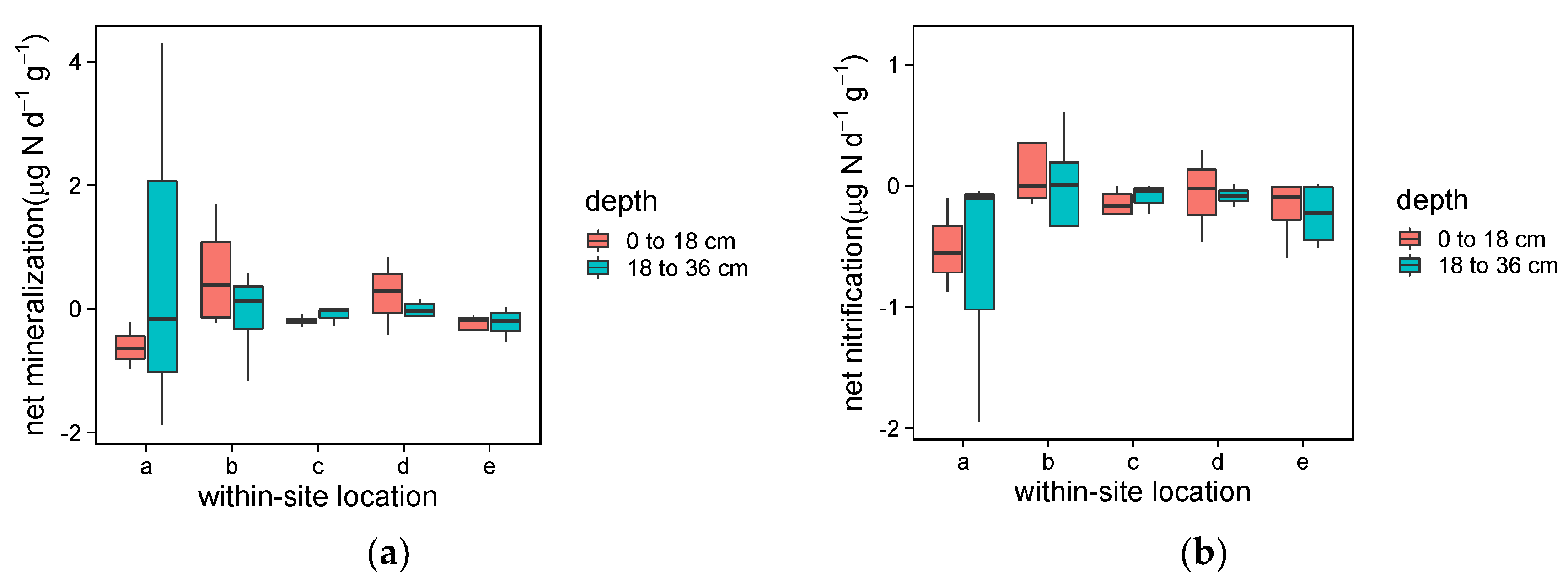
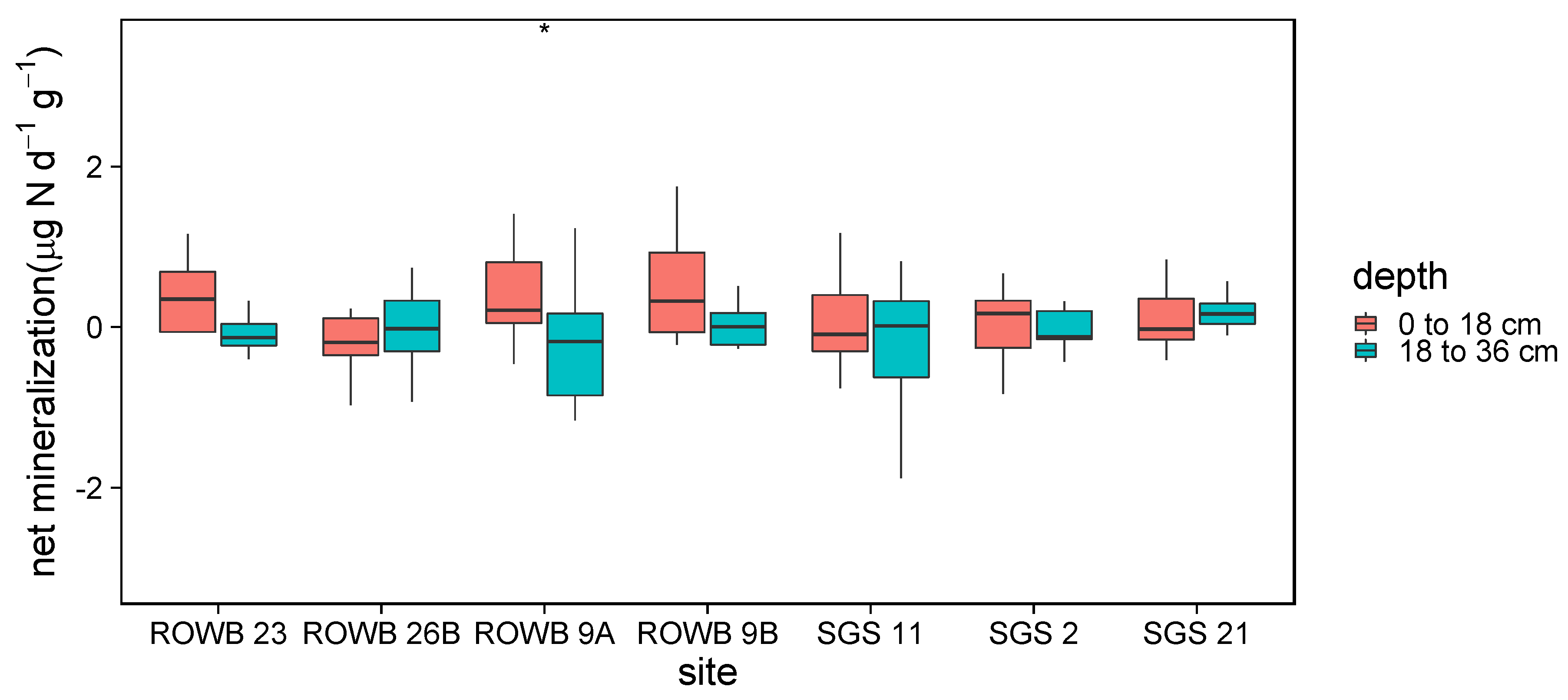
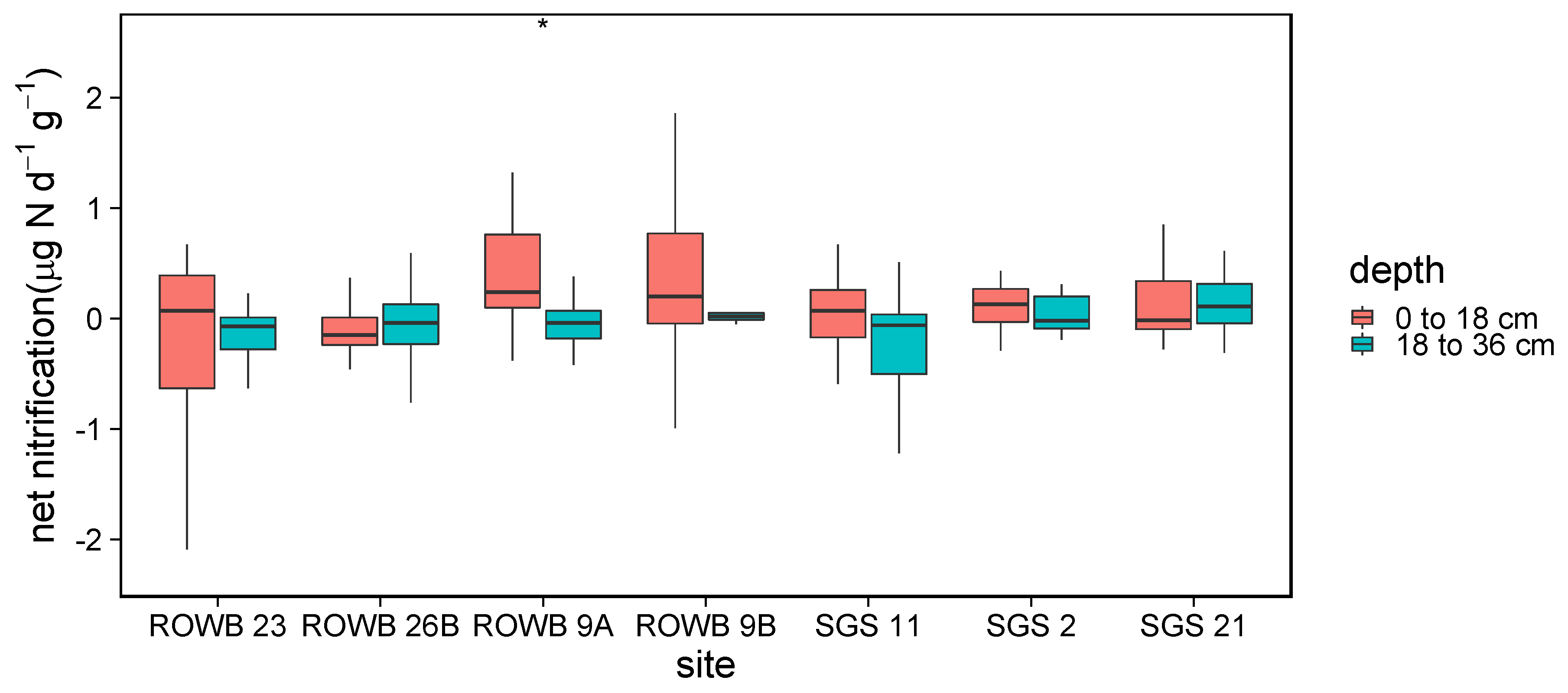
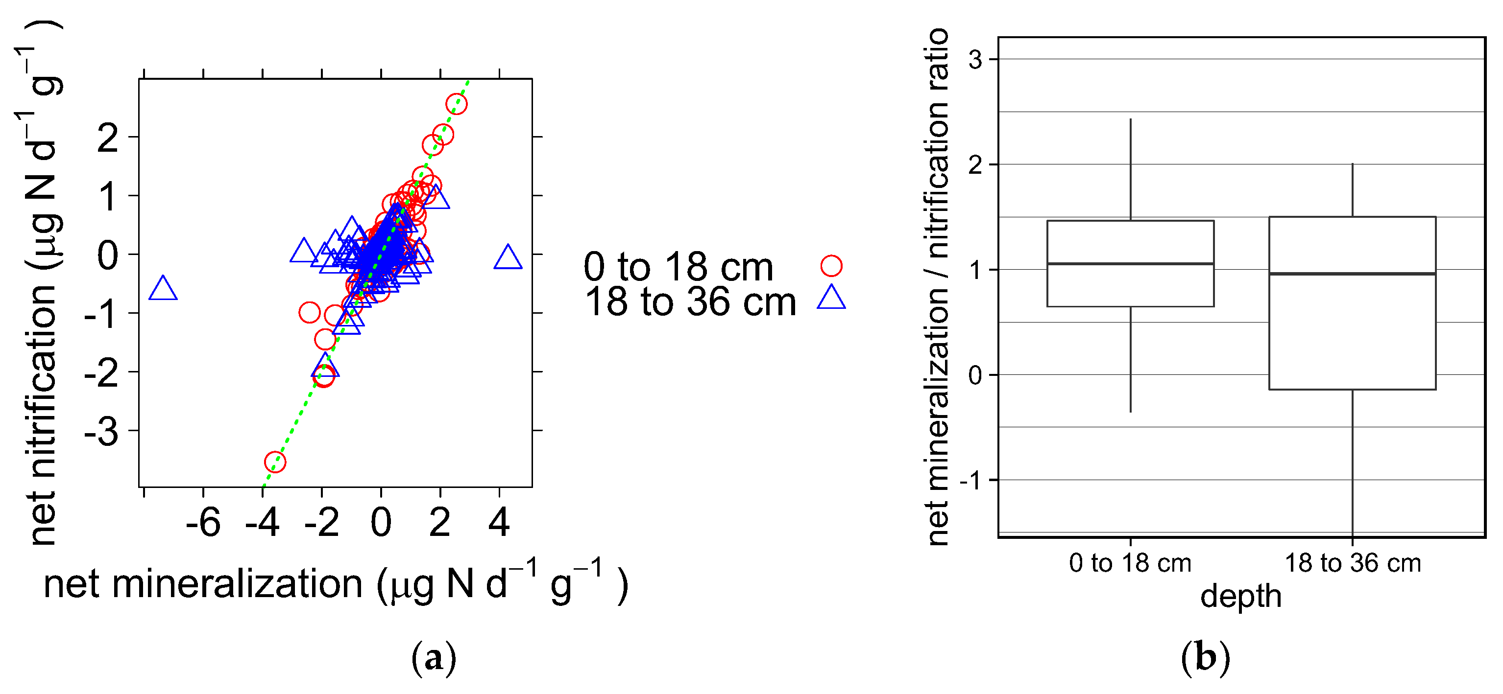
3.1.2. Soil Mineralization and Nitrification

Although the core housings were 50.8 cm in length, the average soil core length during the 15-month monitoring period was 36.5 cm, because 5 cm of the core housing was above ground and the soil core itself would often compact during sampling. Consequently, the shallow and deep halves of soil cores averaged 18.25 cm each.
Soil inorganic nitrogen concentrations and transformation rates were more impacted by the depth than placement within the bioswale. The five soil cores evenly spaced down the length of the four sites (ROWB 26B, ROWB 9B, SGS 11, SGS 21), which were used to test within-site spatial variability from bioswale inlet to outlet, did not demonstrate an increasing or decreasing trend for soil nitrate (p = 0.127, n = 75), ammonium (p = 0.533, n = 75), mineralization (p = 0.939, n = 36), or nitrification (p = 0.639, n = 36) (Figure 3).
On the other hand, the shallow halves of soil cores for all sites overall had greater nitrate (p = 0.008, n = 423), mineralization (p = 0.044, n = 209) and nitrification (p = 0.043, n = 209) compared to the deep halves, but had no overall difference for ammonium (p = 0.131, n = 423).
The seven different sites produced similar results to one another (Figure 4 and Figure 5), although site ROWB 23 had the most soil inorganic nitrogen in soil extracts, with statistically greater concentrations of extractable ammonium than SGS 21 (p = 0.019, n = 119) and SGS 11 (p = 0.047, n = 119). ROWB 23 also had greater extractable nitrate than SGS 21 (p = 0.006, n = 119), SGS 2 (p = 0.011, n = 104), and ROWB 9B (p = 0.014, n = 117). Inorganic nitrogen concentrations, mineralization, and nitrification rates did not show statistically significant differences (p < 0.05) among the other sites. Within each site, the shallow halves had statistically greater nitrification and mineralization for site ROWB 9A only.
Soil extractable ammonium displayed a seasonal trend, as the greatest ammonium concentrations occurred in the summer (Figure 6). Specifically, June 2015 demonstrated statistically greater ammonium concentrations than every other period, with the exception of June 2016. The other dates were not statistically different from one another. June 2015 was also the only period with statistically significant differences between initial and incubated concentrations.
While soil extractable nitrate concentrations also displayed a possible seasonal trend, as the lowest nitrate concentrations were found in the cooler months of November and March 2016 (Figure 7), nitrate levels were more affected by precipitation. The only statistically significant increase between initial and incubated soil levels for nitrate occurred in September 2015 and December 2015, when rain did not occur during the incubation period. In contrast, in June 2016 there was a clear decrease between initial and incubated soil levels for nitrate, as this period had the greatest rain depth (Figure 7). Ammonium levels however showed mostly seasonal variability (Figure 6).
One of the greatest net nitrification rates was found during the rain-free period of September, 2015 (Table 3), and the lowest rate was found during June 2016, when there was the largest rain amount. However, there were no consistent patterns in mineralization rates among sampling periods (Table 3). There was no increasing or decreasing trend over time from 2015 to 2016 for mineralization (p = 0.502, n = 209) or nitrification (p = 0.470, n = 209).
Soil mineralization and nitrification followed a “one to one” relationship, especially for shallow soils (Figure 8). This ratio implies that nearly all organic nitrogen was eventually transformed into nitrate, because ammonium resulting from mineralization was quickly nitrified and stored as nitrate. Shallow samples generally had greater nitrification than deeper samples (Figure 8a). The full soil data are found in the Supplemental Material.

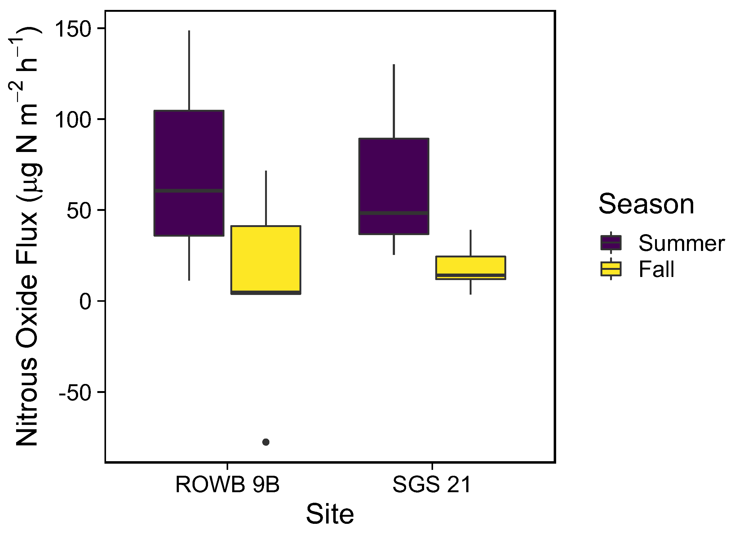
3.2. Soil Gas Emissions
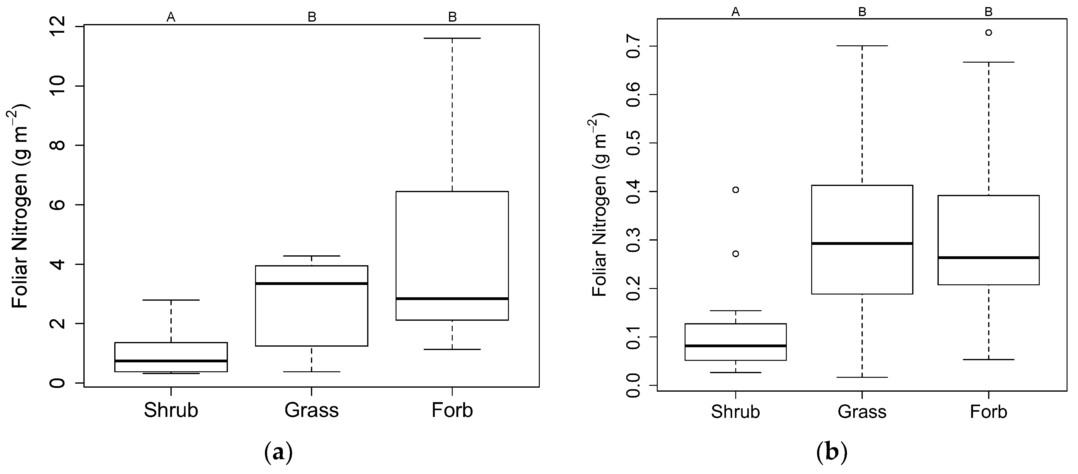
Soil N2O gas emissions overall averaged 35 μg N2O-N m−2 h−1, with a maximum of 149 μg N2O-N m−2 h−1, and one negative flux (N2O consumption) of −78 μg N2O-N m−2 h−1. As shown in Figure 9, the two sites where gases were sampled were not statistically different from each other (p = 0.959) but the six measured summer fluxes were statistically greater than the ten fall fluxes (p = 0.042). There were neither significant correlations with 3-day antecedent rain (p = 0.515) nor with temperature (p = 0.081). The full gas data are found in the Supplemental Material.

3.3. Plant Uptake

The shrubs, including Rosa ‘Radrazz’ Knockout, Spiraea tomentosa, and Aronia melanocarpa, had lower foliar nitrogen per bioswale area (Figure 10a) than the grasses (p = 0.003), which included Panicum virgatum and Pennisetum alopecuroides, and the forbs (p = 0.0001), which included Echinacaea purpurea, Hemerocallis ‘Lady Florence’, Symphyotrichum novae-angliae, Liriope muscari, and Nepeta faassennii. The grasses and forbs did not show statistically significant differences for foliar nitrogen per bioswale area (p = 0.333). Hemerocallis had the most, averaging 8.0 g N m−2, with a maximum of 11.6 g N m−2.
The shrubs also had about one-third lower nitrogen on a per leaf area basis (Figure 10b) than the grasses (p < 0.0001) and the forbs (p < 0.0001). Shrub leaves had an average C:N ratio of 28.5, which was greater than the grass leaves average ratio of 20.4 (p = 0.0003), and the forb leaves average ratio of 16.7 (p < 0.0001). The only index where shrubs indicated greater uptake was patch area, for which the shrubs averaged 0.5 m2, while the shrubs and grasses each averaged 0.4 m2, although patch area for shrubs was neither statistically greater than patch area for the grasses (p = 0.539) or the forbs (p = 0.408).
Total foliar nitrogen for shrubs, grasses, and forbs at the four sites averaged 30.2 g N and the trees contained an additional 14.1 g N on average. Total nitrogen content in aboveground foliage at the 9.3 m2 sites averaged 4.8 g N m−2. The full plant data are found in the Supplemental Material.

4. Discussion

4.1. Soil

4.1.1. Soil Characterization

Our data quantify nitrogen cycling in the soil, gas, and plant phase. These are poorly documented fluxes of the bioswale nitrogen cycle that occur during dry weather. In particular, the data indicate that bioswale soils contain overabundant nitrogen in excess of plant and microbial uptake. As such, the C:N ratios of the soils were below 25:1 (Table 2), which is considered the critical C:N ratio. Above this ratio, microbes may be nitrogen limited and below it there may be net nitrogen release from decomposing organic matter [16,54]. Soils with greater C:N ratios tend to be more capable of removing nitrogen from stormwater by promoting microbial uptake (immobilization) over mineralization [12,21,55,56].

4.1.2. Soil Mineralization and Nitrification

Soil nitrogen concentrations did not vary with sampling location, as there were few differences between sites and no clear spatial trends from the inlet to the outlet. However, shallower bioswale soil samples had greater soil nitrate concentrations, mineralization rates, and nitrification rates compared to deeper soil, which might be expected because inputs from stormwater influent and decomposing plant organic matter increase nitrogen levels in shallow soil. In most soils, the quantity and quality of detrital inputs and fertilization are the main factors that control rates and patterns of mineralization and immobilization [16,36]. Shallow soil is also topped with 7 cm of bark chip mulch, which can remove organic nitrogen from stormwater runoff through sorption processes, and also support substantial microbe populations to mineralize and nitrify captured organic nitrogen between rain events [10].
Moreover, shallow soils experience greater temperature fluctuations, supporting faster decomposition than found in deeper soil [57]. Likewise, moisture levels and temperature are more stable in the subsoil [58], and deeper soils retain less carbon and nitrogen [7]. There are also increased oxygen levels closer to the surface, supporting autotrophic nitrification and aerobic metabolism, which are aerobic processes. Other bioswale monitoring studies found most total nitrogen [59] and nitrate [60] to be produced in shallow soils, suggesting that nitrification mainly occurs in the upper soil layers.
The overabundance of nitrogen in shallow soils is also evidenced by the 1:1 relationship between net mineralization and net nitrification in Figure 8a,b. Our research shows that in urban bioswales, nitrogen accumulates as nitrate, rarely as ammonium. Net nitrification is typically 100% of net mineralization in nitrogen-abundant tropical ecosystems [61] and agricultural systems [13], while only a small fraction of net mineralization in temperate ecosystems [62], because nitrifying microbes thrive in nitrogen-abundant environments, but compete poorly for ammonium against plants and heterotrophic microbes when nitrogen is scarce. In nitrogen-abundant environments, nitrifiers live in close association with mineralizers, making nitrate the dominant nitrogen form moving through the soil, and plants rely on nitrate for nitrogen [13]. However, gross rates of nitrification exceed rates of nitrate uptake by plants and microorganisms, resulting in the accumulation of nitrate; this indicates that excess nitrogen is cycling relative to the ability of plants and microbes to assimilate it [22]. Our data suggest that bioswale soils supply much more nitrogen than the plants need, especially at shallow depths. The excess nitrogen may not only originate from the initial soil design, but also from inputs from stormwater nitrogen and decomposing plant organic nitrogen that the soil makes available through mineralization and nitrification.
We also found that the overabundance of nitrogen increased in warmer months, as indicated by greater concentrations of ammonium in the summer (Figure 6). Warmer weather stimulates the mineralization process [63,64], and a similar trend is visible in grassland ecosystems, which show increased ammonium and nitrate concentrations in the summer and decreased concentrations in the fall [65]. Compared to ammonium levels, levels of nitrate fluctuated greatly through high rates of accumulation and leaching (Figure 7 and Figure 8a). The lower left quadrant of Figure 8a shows a tight relationship between mineralization and nitrification rates, indicating only nitrate levels to be decreasing, as nitrate is a highly mobile anion that does not bind to soil particles and so is readily washed out [10,16], whereas ammonium is stable.

4.2. Soil Gas Emissions

We also found greater nitrous oxide emissions in summer than fall. This increase might be due to the connection between warmer temperatures and high rates of nitrous oxide gas emissions from nitrification and denitrification [27,66]. High levels of ammonium in the soil also leads to increased nitrification and denitrification [15,54], so the summer’s increase in ammonium (Figure 6) possibly further increased summer gas emissions of nitrous oxide.
Our results might be applicable to bioswales in other cities because the levels of nitrous oxide emitted by our bioswales were similar to rates found in similar studies around the world: our mean reported N2O flux of 35 μg N m−2 h−1 was in the mid-range, as per the mean N2O fluxes of 13.8 and 65.6 μg N2O-N m−2 h−1 found in two bioswales in Melbourne, Australia [24], the 23.4 μg of N2O-N m−2 h−1 found in a bioswale in New York, USA [21], and the 10 μg of N2O-N m−2 h−1 found in bioswales in Vermont, USA [67]. Our peak emissions of 148.6 μg N2O-N m−2 h−1 were lower than the peak of 1100 μg N2O-N m−2 h−1 found by Grover et al. [24] and the 330 μg of N2O-N m−2 h−1 found by Shrestha et al. [67], but similar to the 125 μg N2O-N m−2 h−1 found by McPhillips et al. [21].

4.3. Plant Uptake

Compared to the forbs and grasses, the leaves of the shrubs had lower nitrogen per site area, lower nitrogen per leaf area, and greater C:N ratios, all showing a lower rate of nitrogen uptake. While Collins et al. [5] suggested that trees and shrubs may remove more nitrogen in the long run due to deeper rooting systems and greater biomass, Turk et al. [68] found that herbaceous perennials outperformed trees and shrubs on nitrogen removal per unit area. Plants with the most nitrogen removal grow rapidly in nitrogen-rich environments and have the ability to store excess nitrogen [59]. Perhaps the grasses and perennial herbs were growing more rapidly, while the shrubs were storing excess nitrogen in woody biomass [32], which was not sampled in this study.

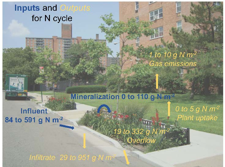
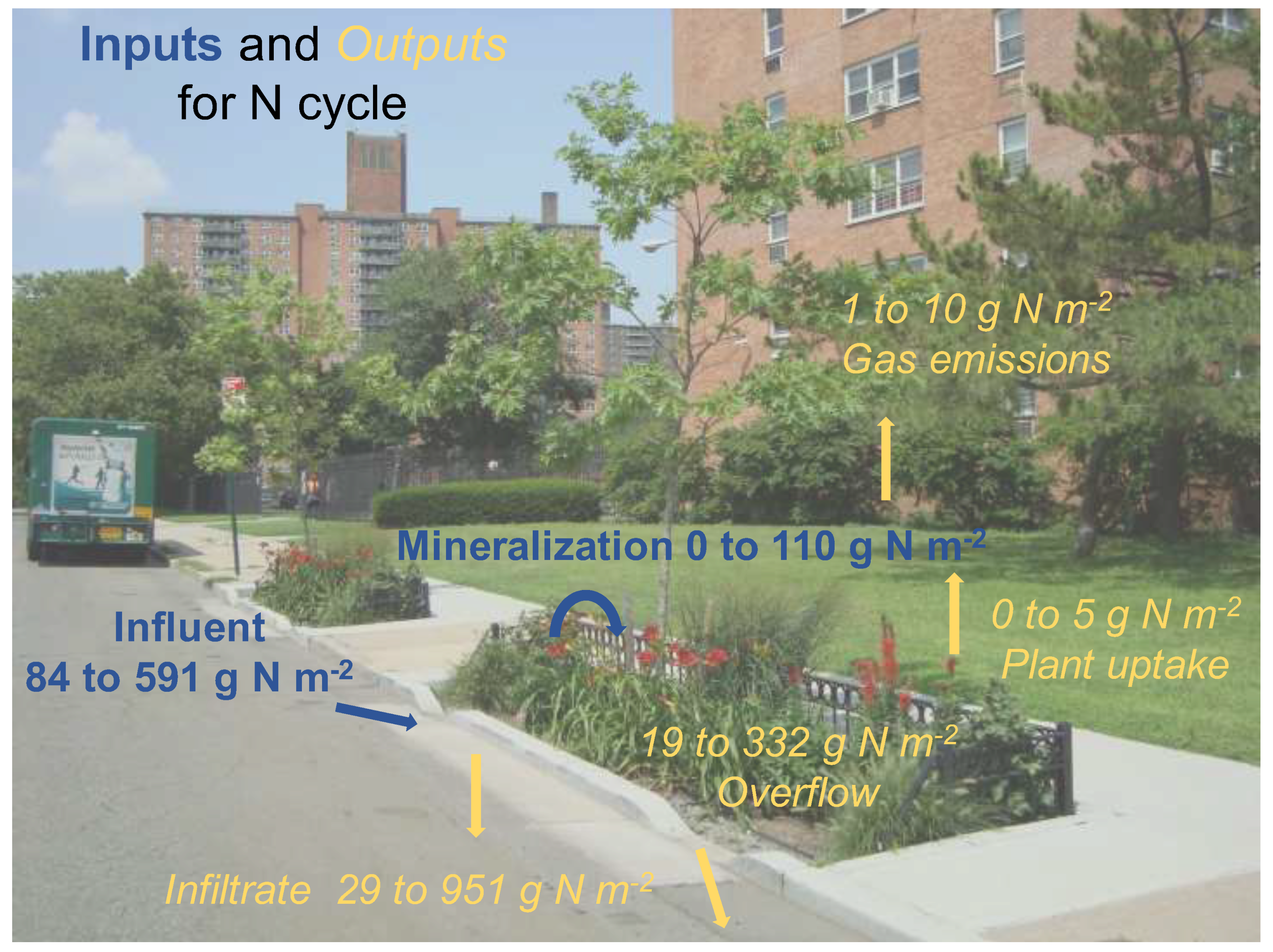
4.4. Nitrogen Mass Balance

We estimated minimum and maximum fluxes for each aspect of the nitrogen cycle by extrapolating from our measurements with results from other literature as explained in the Supplemental Material. We found that soil mineralization amounted to 0 to 110 g N m−2 y−1, gas losses were 1 to 10 g N m−2 y−1, and plant uptake was 0 to 5 g N m−2 y−1. We also compared our results to water measurements conducted at the same sites, also as explained in the Supplemental Material. Stormwater influent added 84 to 591 g N m−2 y−1, while 29 to 951 g N m−2 y−1 infiltrated via stormwater into the subsoil, and 19 to 332 g N m−2 y−1 overflowed back into the sewer system (Figure 11).
Thus, bioswale nitrogen cycling is dominated by liquid and soil phase fluxes, with relatively much smaller fluxes in the gas and plant phases. In contrast to natural ecosystems, where external inputs of nitrogen are about 10% of the amount of nitrogen that annually cycles [54], stormwater inputs of nitrogen in the studied urban bioswales constitute most of the nitrogen that annually cycles. We found that gas emissions were a small portion of the overall mass balance, which was similar to findings by Payne et al. [69] and Morse et al. [70], who found that N2O emissions were only 1 to 2% of the incoming nitrogen amount.

4.5. Limitations

Our mineralization data were limited by periodic rains washing away accumulated nitrate, preventing a clear measurement of inorganic nitrogen changes. However, this condition allowed us to contrast the fluctuating changes of soil nitrate due to leaching with the more gradual seasonal changes of soil ammonium. Future research could quantify such washouts by sealing off the top and bottom of incubated soil cores with ion exchange resin bags, which prevent loss of ammonium and nitrate [37], and would clarify the negative fluxes we often found for mineralization and nitrification due to rainfall.
The act of taking net mineralization measurements has the side effect of cutting soil roots with the sharpened edge of the soil corer, eliminating plant uptake of nitrogen sources, which alters the nitrogen system, enabling higher microbe uptake and lower net mineralization [13]. In addition, the soil core may sever roots that nevertheless may continue to take up nitrogen within the core, again resulting in underestimates of net mineralization [14,36]. On the other hand, the incubated core may have slightly greater soil moisture than the rest of the site [13,37], potentially leading to overestimates of the mineralization rate [57]. Ultimately, no method for assessing soil nitrogen provides an unequivocal estimate [37]. Our intact soil core method may reduce soil disturbance compared to other field methods of quantifying soil mineralization, which are more reliable than laboratory incubations [36].
We found that nitrogen content in aboveground foliage totaled about 5 g m−2. However, plants may store nitrogen in areas other than leaves. Total plant nitrogen uptake per year could be much greater, as a study found wetland plant nitrogen uptake levels to be 51 g N m−2 y−1 [10], and Lucas and Greenway [17] found that nitrogen uptake ranged from 51 to 65 g N m−2 y−1 for plants grown in lab mesocosms. Future analyses should consider all plant parts, including stems, roots, flowers, pods, and seeds.
As discussed in the Supplemental Material, this study relied on numerous assumptions in generalizing monitored measurements into an annual budget. While our simplifying assumptions limit the precision of our overall estimate, even a conservative estimate of inputs to the studied bioswales in stormwater (84–591 g N m−2 y−1) and mineralization (0–110 g N m−2 y−1) greatly exceed fertilization guidelines (5–20 g N m−2 y−1) [30]. Future research should study how to provide balanced nutrition for vegetation when planted in soil with overabundant nitrogen. Future studies should also test the degree to which plants can absorb the nitrogen in stormwater given that it comes in rapid waves.

4.6. Implications

Bioswale soil could better account for the overabundance of nitrogen within stormwater, in order to reduce nitrogen leaching. Detailed design guidance is not available for bioswales [71], and high organic matter contents are frequently specified for bioswale soil, intended to aid plant growth rather than improve water quality [21,72]. Due to this finding we advocate for more stable and more carbon-based organic matter used in soil mixes to increase the C:N ratio for better nitrogen management.
The engineered soil specification for NYC bioswales (Supplemental Materials) specifies leaf compost as the only approved amendment to achieve the required organic matter content of 3 to 8%. While leaf compost is already high in carbon, the soil specification could further require that compost stability meet a requirement, such as (1) a Solvita maturity index score of 7 or 8 [30,73], or (2) less than 3 mg CO2-C per g compost organic matter per day [74,75]. Furthermore, the soil specification total nitrogen maximum of 0.25% could be reduced to the 0.15% levels we found in situ (Table 2), given that the levels in our study were nitrogen rich.
Our data indicate that stormwater and mineralization inputs of nitrogen are more than enough to promote healthy vegetation. A less nitrogen rich soil composition with stable soil carbon enhancements such as coconut coir pith as a replacement for compost [76] might enhance long-term net immobilization in order to reduce nitrogen leaching. We also suggest that the bioswales be maintained without additional fertilizers.
Although plant health was not quantified in this study, excess nitrogen is not only linked with increased pollution, but even with declines in forest productivity and increased tree mortality [54]. Surplus fertilizer promotes shoot growth and diverts resources from root growth and production of defensive chemicals, which decreases drought tolerance and pest resistance [77]. When planted in a less nitrogen rich soil, native plants may also better outcompete weeds, potentially reducing maintenance [78]. Our recommendations may therefore support healthier plants with reduced maintenance, in addition to decreasing urban sources of nitrogen pollution.

Supplementary Materials

The following are available online at https://www.mdpi.com/2073-4441/10/11/1627/s1.

Author Contributions

Conceptualization, N.S., D.N.L.M., K.M., and P.C.; Formal analysis, N.S., B.M., and P.C.; Funding acquisition, P.C.; Investigation, N.S., R.H., J.H., and B.M.; Methodology, N.S., R.H., B.M., M.P., D.N.L.M., K.M., and W.M.; Project administration, P.C.; Resources, B.M., M.P., D.N.L.M., and P.C.; Supervision, B.M., M.P., and P.C.; Writing—original draft, N.S.; Writing—review and editing, R.H., J.H., B.M., M.P., D.N.L.M., K.M., and P.C.

Funding

This work was funded, in part, by the National Science Foundation awards CMMI-1325676 and CBET-1444745, and the Environmental Protection Agency contract EP-15-C-000016.

Acknowledgments

The authors wish to thank the NYC Department of Parks & Recreation and the NYC Department of Environmental Protection for supporting our monitoring work. Any opinions, findings, and conclusions expressed in this paper are those of the authors and not meant to represent the views of any supporting institution.

Conflicts of Interest

The authors declare no conflicts of interest.

References

  1. Howarth, R.W.; Marino, R. Nitrogen as the Limiting Nutrient for Eutrophication in Coastal Marine Ecosystems: Evolving Views over Three Decades. Limnol. Oceanogr. 2006, 51, 364–376. [Google Scholar] [CrossRef]
  2. Bettez, N.D.; Groffman, P.M. Nitrogen Deposition in and near an Urban Ecosystem. Environ. Sci. Technol. 2013, 47, 6047–6051. [Google Scholar] [CrossRef] [PubMed]
  3. Clar, M.; Green, R. Design Manual for Use of Bioretention in Stormwater Management; Department of Environmental Resources: Prince George’s County, MD, USA, 1993. [Google Scholar]
  4. Bratieres, K.; Fletcher, T.D.; Deletic, A.; Zinger, Y. Nutrient and Sediment Removal by Stormwater Biofilters: A Large-Scale Design Optimisation Study. Water Res. 2008, 42, 3930–3940. [Google Scholar] [CrossRef] [PubMed]
  5. Collins, K.A.; Lawrence, T.J.; Stander, E.K.; Jontos, R.J.; Kaushal, S.S.; Newcomer, T.A.; Grimm, N.B.; Cole Ekberg, M.L. Opportunities and Challenges for Managing Nitrogen in Urban Stormwater: A Review and Synthesis. Ecol. Eng. 2010, 36, 1507–1519. [Google Scholar] [CrossRef]
  6. Hunt, W.F.; Jarrett, A.R.; Smith, J.T.; Sharkey, L.J. Evaluating Bioretention Hydrology and Nutrient Removal at Three Field Sites in North Carolina. J. Irrig. Drain. Eng. 2006, 132, 600–608. [Google Scholar] [CrossRef] [Green Version]
  7. Li, L.; Davis, A.P. Urban Stormwater Runoff Nitrogen Composition and Fate in Bioretention Systems. Environ. Sci. Technol. 2014, 48, 3403–3410. [Google Scholar] [CrossRef] [PubMed]
  8. Passeport, E.; Hunt, W.F. Asphalt Parking Lot Runoff Nutrient Characterization for Eight Sites in North Carolina, USA. J. Hydrol. Eng. 2009, 14, 352–361. [Google Scholar] [CrossRef]
  9. Peterson, I.J.; Igielski, S.; Davis, A.P. Enhanced Denitrification in Bioretention Using Woodchips as an Organic Carbon Source. J. Sustain. Water Built Environ. 2015, 9, 1–9. [Google Scholar] [CrossRef]
  10. Davis, A.P.; Shokouhian, M.; Sharma, H.; Minami, C. Water Quality Improvement through Bioretention Media: Nitrogen and Phosphorus Removal. Water Environ. Res. 2006, 78, 284–293. [Google Scholar] [CrossRef] [PubMed]
  11. McNett, J.K.; Hunt, W.F.; Davis, A.P. Influent Pollutant Concentrations as Predictors of Effluent Pollutant Concentrations for Mid-Atlantic Bioretention. J. Environ. Eng. 2011, 137, 790–799. [Google Scholar] [CrossRef]
  12. Payne, E.G.I.; Fletcher, T.D.; Cook, P.L.M.; Deletic, A.; Hatt, B.E. Processes and Drivers of Nitrogen Removal in Stormwater Biofiltration. Crit. Rev. Environ. Sci. Technol. 2014, 44, 796–846. [Google Scholar] [CrossRef]
  13. Schimel, J.P.; Bennett, J. Nitrogen Mineralization: Challenges of a Changing Paradigm. Ecology 2004, 85, 591–602. [Google Scholar] [CrossRef]
  14. Robertson, P.G.; Wedin, D.; Groffman, P.M.; Blair, J.M.; Holland, E.A.; Nadelhoffer, K.J.; Harris, D. Soil Carbon and Nitrogen Availability: Nitrogen Mineralization, Nitrification, and Soil Respiration Potentials. In Standard Soil Methods for Long-Term Ecological Research; Robertson, G.P., Bledsoe, C.S., Coleman, D.C., Sollins, P., Eds.; Oxford University Press: New York, NY, USA, 1999; pp. 258–271. [Google Scholar]
  15. Groffman, P.M.; Boulware, N.J.; Zipperer, W.C.; Pouyat, R.V.; Band, L.E.; Colosimo, M.F. Soil Nitrogen Cycle Processes in Urban Riparian Zones. Environ. Sci. Technol. 2002, 36, 4547–4552. [Google Scholar] [CrossRef] [PubMed]
  16. Robertson, G.P.; Groffman, P.M. Chapter 14—Nitrogen Transformations. In Soil Microbiology Ecology and Biochemistry; Elsevier Inc.: Amsterdam, The Netherlands, 2015; pp. 421–446. [Google Scholar]
  17. Lucas, W.C.; Greenway, M. Hydraulic Response and Nitrogen Retention in Bioretention Mesocosms with Regulated Outlets: Part II—Nitrogen Retention. Water Environ. Res. 2011, 83. [Google Scholar] [CrossRef]
  18. Shetty, N.H.; Culligan, P.J.; Mailloux, B.; McGillis, W.R.; Do, H.Y. Bioretention Infrastructure to Manage the Nutrient Runoff from Coastal Cities. In Geo-Chicago 2016 GSP 273; ASCE: Reston, VA, USA, 2016; pp. 402–411. [Google Scholar]
  19. Brown, R.A.; Birgand, F.; Hunt, W.F. Analysis of Consecutive Events for Nutrient and Sediment Treatment in Field-Monitored Bioretention Cells. Water Air Soil Pollut. 2013, 224, 1581. [Google Scholar] [CrossRef]
  20. Lucas, W.C.; Greenway, M. Nutrient Retention in Vegetated and Nonvegetated Bioretention Mesocosms. J. Irrig. Drain. Eng. 2008, 134, 613–623. [Google Scholar] [CrossRef]
  21. McPhillips, L.; Goodale, C.; Walter, M.T. Nutrient Leaching and Greenhouse Gas Emissions in Grassed Detention and Bioretention Stormwater Basins. J. Sustain. Water Built Environ. 2018, 4, 1–10. [Google Scholar] [CrossRef]
  22. Davidson, E.A.; Keller, M.; Erickson, H.E.; Verchot, L.V.; Veldkamp, E. Testing a Conceptual Model of Soil Emissions of Nitrous and Nitric Oxides. Bioscience 2000, 50, 667. [Google Scholar] [CrossRef] [Green Version]
  23. Templer, P.H.; Pinder, R.W.; Goodale, C.L. Effects of Nitrogen Deposition on Greenhouse-Gas Fluxes for Forests and Grasslands of North America. Front. Ecol. Environ. 2012, 10, 547–553. [Google Scholar] [CrossRef]
  24. Grover, S.P.P.; Cohan, A.; Chan, H.S.; Livesley, S.J.; Beringer, J.; Daly, E. Occasional Large Emissions of Nitrous Oxide and Methane Observed in Stormwater Biofiltration Systems. Sci. Total Environ. 2013, 465, 64–71. [Google Scholar] [CrossRef] [PubMed]
  25. McPhillips, L.E.; Groffman, P.M.; Schneider, R.L.; Walter, M.T. Nutrient Cycling in Grassed Roadside Ditches and Lawns in a Suburban Watershed. J. Environ. Qual. 2016, 45, 1901. [Google Scholar] [CrossRef] [PubMed]
  26. Oertel, C.; Matschullat, J.; Zurba, K.; Zimmermann, F.; Erasmi, S. Greenhouse Gas Emissions from Soils—A Review. Chem. Erde Geochem. 2016, 76, 327–352. [Google Scholar] [CrossRef]
  27. Livesley, S.J.; Dougherty, B.J.; Smith, A.J.; Navaud, D.; Wylie, L.J.; Arndt, S.K. Soil-Atmosphere Exchange of Carbon Dioxide, Methane and Nitrous Oxide in Urban Garden Systems: Impact of Irrigation, Fertiliser and Mulch. Urban Ecosyst. 2010, 13, 273–293. [Google Scholar] [CrossRef]
  28. Townsend-Small, A.; Czimczik, C.I. Carbon Sequestration and Greenhouse Gas Emissions in Urban Turf. Geophys. Res. Lett. 2010, 37, 1–5. [Google Scholar] [CrossRef]
  29. Townsend-Small, A.; Pataki, D.E.; Czimczik, C.I.; Tyler, S.C. Nitrous Oxide Emissions and Isotopic Composition in Urban and Agricultural Systems in Southern California. J. Geophys. Res. 2011, 116, G01013. [Google Scholar] [CrossRef]
  30. Goatley, M.; Hensler, K. Urban Nutrient Management Handbook; Virginia Cooperative Extension: Petersburg, VA, USA, 2011. [Google Scholar]
  31. Roy-Poirier, A.; Champagne, P.; Filion, Y. Review of Bioretention System Research and Design: Past, Present, and Future. J. Environ. Eng. 2010, 136, 878–889. [Google Scholar] [CrossRef]
  32. Payne, E.; Fletcher, T.D.; Russell, D.G.; Grace, M.R.; Cavagnaro, T.R.; Evrard, V.; Deletic, A.; Hatt, B.E.; Cook, P.L.M. Temporary Storage or Permanent Removal? The Division of Nitrogen between Biotic Assimilation and Denitrification in Stormwater Biofiltration Systems. PLoS ONE 2014, 9, e90890. [Google Scholar] [CrossRef] [PubMed]
  33. Gilchrist, S.; Borst, M.; Stander, E.K. Factorial Study of Rain Garden Design for Nitrogen Removal. J. Irrig. Drain. Eng. 2014, 140, 04013016. [Google Scholar] [CrossRef]
  34. Shetty, N.H. New York City’s Green Infrastructure: Impacts on Nutrient Cycling and Improvements in Performance. Ph.D. Thesis, Columbia University, New York, NY, USA, 2018. [Google Scholar]
  35. ASTM. Standard Practice for Soil Exploration and Sampling by Auger Borings D1452/D1452M—16; ASTM: West Conshohocken, PA, USA, 2016; pp. 3–9. [Google Scholar]
  36. Raison, R.J.; Connel, M.J.; Khanna, P.K. Methodology for Studying Fluxes of Soil Mineral-N in Situ. Soil Biol. Biochem. 1987, 19, 521–530. [Google Scholar] [CrossRef]
  37. Hart, S.C.; Stark, J.M.; Davidson, E.A.; Firestone, M.K. Nitrogen Mineralization, Immobilization, and Nitrification. In Methods of Soil Analysis, Part 2. Microbiological and Biochemical Properties; Weaver, R.W., Angle, J.S., Bottomley, P.J., Bezdiek, D.F., Smith, M.S., Tabatabai, M.A., Eds.; Soil Science Society of America: Madison, WI, USA, 1994; pp. 985–1018. [Google Scholar]
  38. Klute, A. Methods of Soil Analysis: Part 1—Physical and Mineralogical Methods, 2nd ed.; Soil Science Society of America: Madison, WI, USA, 1986; Volume 9. [Google Scholar]
  39. Holmes, R.M.; Aminot, A.; Kerouel, R.; Hooker, B.A.; Peterson, B.J. A Simple and Precise Method for Measuring Ammonium in Marine and Freshwater Ecosystems. Can. J. Fish. Aquat. Sci. 1999, 56, 1801–1808. [Google Scholar] [CrossRef]
  40. US EPA. Method 9056A Determination of Inorganic Anions by Ion Chromatography. 2007; No. February; pp. 1–19. [Google Scholar]
  41. Pihlatie, M.K.; Christiansen, J.R.; Aaltonen, H.; Korhonen, J.F.J.; Nordbo, A.; Rasilo, T.; Benanti, G.; Giebels, M.; Helmy, M.; Sheehy, J.; et al. Comparison of Static Chambers to Measure CH4 Emissions from Soils. Agric. For. Meteorol. 2013, 171–172, 124–136. [Google Scholar] [CrossRef]
  42. Norton, R.A.; Harrison, J.A.; Kent Keller, C.; Moffett, K.B. Effects of Storm Size and Frequency on Nitrogen Retention, Denitrification, and N2O Production in Bioretention Swale Mesocosms. Biogeochemistry 2017, 134, 353–370. [Google Scholar] [CrossRef]
  43. Sonnentag, O.; Talbot, J.; Chen, J.M.; Roulet, N.T. Using Direct and Indirect Measurements of Leaf Area Index to Characterize the Shrub Canopy in an Ombrotrophic Peatland. Agric. For. Meteorol. 2007, 144, 200–212. [Google Scholar] [CrossRef]
  44. Trammell, T.L.; Ralston, H.A.; Scroggins, S.A.; Carreiro, M.M. Foliar Production and Decomposition Rates in Urban Forests Invaded by the Exotic Invasive Shrub, Lonicera Maackii. Biol. Invasions 2012, 14, 529–545. [Google Scholar] [CrossRef]
  45. Xu, C.Y.; Griffin, K.L.; Schuster, W.S.F. Leaf Phenology and Seasonal Variation of Photosynthesis of Invasive Berberis Thunbergii (Japanese Barberry) and Two Co-Occurring Native Understory Shrubs in a Northeastern United States Deciduous Forest. Oecologia 2007, 154, 11–21. [Google Scholar] [CrossRef] [PubMed]
  46. Madakadze, I.C.; Stewart, K.; Peterson, P.R.; Coulman, B.E.; Samson, R.; Smith, D.L. Light Interception, Use-Efficiency and Energy Yield of Switchgrass (Panicum virgatum L.) Grown in a Short Season Area. Biomass Bioenergy 1998, 15, 475–482. [Google Scholar] [CrossRef]
  47. Zeri, M.; Anderson-Teixeira, K.; Hickman, G.; Masters, M.; DeLucia, E.; Bernacchi, C.J. Carbon Exchange by Establishing Biofuel Crops in Central Illinois. Agric. Ecosyst. Environ. 2011, 144, 319–329. [Google Scholar] [CrossRef]
  48. Kiniry, J.R.; Anderson, L.C.; Johnson, M.V.; Behrman, K.D.; Brakie, M.; Burner, D.; Hawkes, C. Perennial Biomass Grasses and the Mason–Dixon Line: Comparative Productivity across Latitudes in the Southern Great Plains. Bioenergy Res. 2013, 6, 276–291. [Google Scholar] [CrossRef]
  49. Mitchell, R.B.; Moser, L.E.; Moore, K.J.; Redfearn, D.D. Tiller Demographics and Leaf Area Index of Four Perennial Pasture Grasses. Agron. J. 1998, 90, 47–53. [Google Scholar] [CrossRef] [Green Version]
  50. Redfearn, D.D.; Moore, K.J.; Vogel, K.P.; Waller, S.S.; Mitchell, R.B. Canopy Architecture and Morphology of Switchgrass Populations Differing in Forage Yield. Agron. J. 1997, 89, 262–269. [Google Scholar] [CrossRef]
  51. Boyd, N.S.; Gordon, R.; Martin, R.C. Relationship between Leaf Area Index and Ground Cover in Potato under Different Management Conditions. Potato Res. 2002, 45, 117–129. [Google Scholar] [CrossRef]
  52. Gordon, R.; Brown, D.M.; Dixon, M.A. Estimating Potato Leaf Area Index for Specific Cultivars. Potato Res. 1997, 40, 251–266. [Google Scholar] [CrossRef]
  53. Helsel, D.R.; Hirsch, R.M. Statistical Methods in Water Resources; Elsevier Inc.: Amsterdam, The Netherlands, 2002; Volume 4. [Google Scholar]
  54. Chapin, F.S.; Matson, P.A.; Mooney, H.A. Principles of Terrestrial Ecosystem Ecology; Springer: New York, NY, USA, 2002. [Google Scholar]
  55. Bernot, M.J.; Dodds, W.K. Nitrogen Retention, Removal, and Saturation in Lotic Ecosystems. Ecosystems 2005, 8, 442–453. [Google Scholar] [CrossRef]
  56. Liu, J.; Sample, D.J.; Owen, J.S.; Li, J.; Evanylo, G. Assessment of Selected Bioretention Blends for Nutrient Retention Using Mesocosm Experiments. J. Environ. Qual. 2014, 43, 1754. [Google Scholar] [CrossRef] [PubMed]
  57. Sanaullah, M.; Chabbi, A.; Leifeld, J.; Bardoux, G.; Billou, D.; Rumpel, C. Decomposition and Stabilization of Root Litter in Top- and Subsoil Horizons: What Is the Difference? Plant Soil 2011, 338, 127–141. [Google Scholar] [CrossRef]
  58. Dungait, J.A.J.; Hopkins, D.W.; Gregory, A.S.; Whitmore, A.P. Soil Organic Matter Turnover Is Governed by Accessibility Not Recalcitrance. Glob. Chang. Biol. 2012, 18, 1781–1796. [Google Scholar] [CrossRef]
  59. Zhang, Z.; Rengel, Z.; Liaghati, T.; Antoniette, T.; Meney, K. Influence of Plant Species and Submerged Zone with Carbon Addition on Nutrient Removal in Stormwater Biofilter. Ecol. Eng. 2011, 37, 1833–1841. [Google Scholar] [CrossRef]
  60. Elliott, S.; Meyer, M.H.; Sands, G.R.; Horgan, B. Water Quality Characteristics of Three Rain Gardens Located Within the Twin Cities Metropolitan Area, Minnesota. Cities Environ. 2011, 4, 1–15. [Google Scholar] [CrossRef]
  61. Vitousek, P.M.; Matson, P. Nitrogen Transformations in a Range of Tropical Forest Soils. Soil Biol. Biochem. 1988, 20, 361–367. [Google Scholar] [CrossRef]
  62. McNulty, S.G.; Aber, J.D.; Mclellan, T.M.; Katt, S.M. Nitrogen Cycling in High Elevation Forests of the Northeastern US in Relation to Nitrogen Deposition. Ambio 1990, 19, 38–40. [Google Scholar]
  63. Auyeung, D.S.N.; Suseela, V.; Dukes, J.S. Warming and Drought Reduce Temperature Sensitivity of Nitrogen Transformations. Glob. Chang. Biol. 2013, 19, 662–676. [Google Scholar] [CrossRef] [PubMed]
  64. Nadelhoffer, K.J.; Aber, J.D.; Melillo, J.M. Seasonal Patterns of Ammonium and Nitrate Uptake in Nine Temperate Forest Ecosystems. Plant Soil 1984, 80, 321–335. [Google Scholar] [CrossRef]
  65. Kastovska, E.; Edwards, K.; Picek, T.; Santruckova, H. A Larger Investment into Exudation by Competitive versus Conservative Plants Is Connected to More Coupled Plant-Microbe N Cycling. Biogeochemistry 2015, 122, 47–59. [Google Scholar] [CrossRef]
  66. Hatt, B.E.; Fletcher, T.D.; Deletic, A. Hydrologic and Pollutant Removal Performance of Stormwater Biofiltration Systems at the Field Scale. J. Hydrol. 2009, 365, 310–321. [Google Scholar] [CrossRef]
  67. Shrestha, P.; Hurley, S.E.; Carol Adair, E. Soil Media CO2 and N2O Fluxes Dynamics from Sand-Based Roadside Bioretention Systems. Water 2018, 10, 185. [Google Scholar] [CrossRef]
  68. Turk, R.P.; Kraus, H.T.; Hunt, W.F.; Carmen, N.B.; Bilderback, T.E. Nutrient Sequestration by Vegetation in Bioretention Cells Receiving High Nutrient Loads. J. Environ. Eng. 2017, 143, 06016009. [Google Scholar] [CrossRef]
  69. Payne, E.G.I.; Pham, T.; Cook, P.L.M.; Deletic, A.; Hatt, B.E.; Fletcher, T.D. Inside Story of Gas Processes within Stormwater Biofilters: Does Greenhouse Gas Production Tarnish the Benefits of Nitrogen Removal? Environ. Sci. Technol. 2017, 51, 3703–3713. [Google Scholar] [CrossRef] [PubMed]
  70. Morse, N.R.; McPhillips, L.E.; Shapleigh, J.P.; Walter, M.T. The Role of Denitrification in Stormwater Detention Basin Treatment of Nitrogen. Environ. Sci. Technol. 2017, 51, 7928–7935. [Google Scholar] [CrossRef] [PubMed]
  71. Davis, A.P.; Hunt, W.F.; Traver, R.G.; Clar, M. Bioretention Technology: Overview of Current Practice and Future Needs. J. Environ. Eng. 2009, 135, 109–117. [Google Scholar] [CrossRef]
  72. Hunt, W.F.; Davis, A.P.; Traver, R.G. Meeting Hydrologic and Water Quality Goals through Targeted Bioretention Design. J. Environ. Eng. 2012, 138, 698–707. [Google Scholar] [CrossRef]
  73. Woods End Research Laboratory. Guide to Solvita ® Testing for Compost Maturity Index; Woods End Research Laboratory: Mount Vernon, ME, USA, 2002; Volume 3. [Google Scholar]
  74. Thompson, W.H.; Leege, P.B.; Millner, P.D.; Watson, M.E. Test Methods for the Examination of Composting and Compost (TMECC); Holbrook: New York, NY, USA, 2001. [Google Scholar]
  75. Matteson, T.L.; Sullivan, D.M. Stability Evaluation of Mixed Food Waste Composts. Compost Sci. Util. 2006, 14, 170–177. [Google Scholar] [CrossRef]
  76. Analysis of Bioretention Soil Media for Improved Nitrogen, Phosphorus and Copper Retention; Herrera Environmental Consultants: Seattle, WA, USA, 2015.
  77. Herms, D.A. Understanding Tree Responses to Abiotic and Biotic Stress Complexes. Arborist News 1998, 7, 21–26. [Google Scholar]
  78. Levin, L.A.; Mehring, A.S. Optimization of Bioretention Systems through Application of Ecological Theory. Wiley Interdiscip. Rev. Water 2015, 2, 259–270. [Google Scholar] [CrossRef]
Figure 1. Simplified nitrogen cycle within bioswales: Solid purple arrows denote nitrogen fluxes quantified in this study, while blue dotted arrows denote well-documented liquid-phase fluxes that occur during wet weather only.
Water 10 01627 g001
Figure 2. Photo of representative site with example sampling strategy. Plant sampling locations are omitted from the figure because all plant species were sampled throughout each site.
Water 10 01627 g002
Figure 3. Within-site spatial variability from bioswale inlet to outlet for (a) net mineralization and (b) net nitrification. Nitrogen transformation rates (μg N d−1 g−1 dry soil) as calculated with Equation (1) quantify differences between initial and one-week incubations for shallow and deep halves of soil cores at four bioswales (ROWB 26B, ROWB 9B, SGS 11, SGS 21) (n = 36). “a” denotes the soil cores closest to the inlet, and “e” denotes the soil cores closest to the outlet. ROWB: right-of-way bioswale; SGS: stormwater greenstreet.
Water 10 01627 g003
Figure 4. Net mineralization rates (μg nitrogen (N) d−1 g−1 dry soil) as calculated in Equation (1) quantifying differences between initial and one-week incubations for all soil cores at seven bioswales sampled at two depths (n = 209). * signifies bioswales where shallow (0 to 18 cm) and deep (18 to 36 cm) samples were statistically different. ROWB: right-of-way bioswale; SGS: stormwater greenstreet.
Water 10 01627 g004
Figure 5. Net nitrification rates (μg nitrogen (N) d−1 g−1 dry soil) as calculated in Equation (1) quantifying differences between initial and one-week incubations for all soil cores at seven bioswales sampled at two depths (n = 209). * signifies bioswales where shallow (0 to 18 cm) and deep (18 to 36 cm) samples were statistically different. ROWB: right-of-way bioswale; SGS: stormwater greenstreet.
Water 10 01627 g005
Figure 6. Soil extractable ammonium (parts per million nitrogen (ppm N) g−1 dry soil) in initial and one-week incubations at seven bioswales sampled at two depths monthly (n = 423) from June 2015 to August 2016, omitting two winter months. The letters above represent statistically significant differences among periods (two periods that share a letter are not statistically different), and * signifies periods where initial and incubated samples were statistically different. The bars at the top denote rain amounts during the one-week incubation periods.
Water 10 01627 g006
Figure 7. Soil extractable nitrate (parts per million nitrogen (ppm N) g−1 dry soil) in initial and one-week incubations at seven bioswales sampled at two depths monthly (n = 423) from June, 2015 to August, omitting two winter months. The letters above represent statistically significant differences among periods and * signifies periods where initial and incubated samples were statistically different. The bars at the top denote rain amounts during the one-week incubation periods.
Water 10 01627 g007
Figure 8. Relationship between net nitrogen mineralization and net nitrification (μg nitrogen (N) d−1 g−1 dry soil) for shallow and deep halves of soil cores at seven bioswales (n = 209) (a) Dotted line denotes 1:1 ratio; (b) Net mineralization/nitrification ratio.
Water 10 01627 g008
Figure 9. Soil nitrous oxide gas emissions (n = 16).
Water 10 01627 g009
Figure 10. (a) Foliar nitrogen per bioswale area (n = 42); (b) Foliar nitrogen per leaf area (n = 179). The letters at the top represent statistically significant differences among groups (two groups that share a letter are not statistically different).
Water 10 01627 g010
Figure 11. Approximate nitrogen mass balance with site ROWB 9A in the foreground and site ROWB 9B in the background.
Water 10 01627 g011
Table 1. Bioswale sampling summary. Sites that received more intensive sampling to evaluate within-site spatial variability in soil mineralization and nitrification are designated by “xx”. ROWB: right-of-way bioswale; SGS: stormwater greenstreet.
BioswaleArea (m2)Soil CharacterizationSoil Mineralization and NitrificationGas EmissionsPlant Uptake
ROWB 26B9.3xxx x
ROWB 237.0xx x
ROWB 9A9.3xx x
ROWB 9B9.3xxxxx
SGS 2176.2xxxx
SGS 1194.8xxx
SGS 2115.2xx
Table 2. Soil macronutrient and texture means ± standard error, and Wilcoxon rank-sum test p-values demonstrating lack of statistical difference (p < 0.05) between shallow and deep samples.
DepthTotal N (%)Total C (%)C:N ratioOrganic (%)Sand (%)Silt (%)Clay (%)
7.6–22.9 cm (n = 7)0.15 ± 0.022.9 ± 0.519.4 ± 0.45.0 ± 0.880.1 ± 1.213.4 ± 1.36.5 ± 0.4
30.5–45.7 cm (n = 7)0.13 ± 0.012.4 ± 0.318.7 ± 1.24.1 ± 0.578.6 ± 1.913.5 ± 1.57.9 ± 0.6
p-value0.710.800.220.750.480.950.14
Table 3. Means of net mineralization and net nitrification (μg nitrogen (N) d−1 g−1 dry soil) averaged for shallow and deep halves of soil cores at seven bioswales (n = 209). Letters indicate statistically significant differences among periods.
Month of Incubation PeriodNet Mineralization (µg N d−1 g−1)Net Nitrification (µg N d−1 g−1)
June 2015−0.81b0.01ab
July 20150.68a0.49ab
August 2015−0.11ab−0.05ab
September 20150.02ab0.30a
October 2015−0.11ab−0.31b
November 20150.10ab0.03ab
December 20150.04ab0.11ab
March 20160.23ab0.07ab
April 20160.28ab0.12ab
May 2016−0.05ab0.02ab
June 2016−0.72b−0.50b
July 20160.19ab0.12a
August 20160.20ab0.29ab

