Experimental Study of Overland Flow through Rigid Emergent Vegetation with Different Densities and Location Arrangements

1
Jinyun Forest Ecosystem Research Station, School of Soil and Water Conservation, Beijing Forestry University, Beijing 100083, China
2
Beijing Engineering Research Center of Soil and Water Conservation, Beijing Forestry University, Beijing 100083, China
*
Author to whom correspondence should be addressed.
Water 2018, 10(11), 1638; https://doi.org/10.3390/w10111638
Submission received: 16 October 2018
/
Revised: 8 November 2018
/
Accepted: 8 November 2018
/
Published: 12 November 2018
(This article belongs to the Section Hydraulics and Hydrodynamics)
Abstract
:The effect of vegetation density on overland flow dynamics has been extensively studied, yet fewer investigations have focused on vegetation arrangements with different densities and position features. Flume experiments were conducted to investigate the hydrodynamics of flow through rigid emergent vegetation arranged in combinations with three densities (Dense, Middle, and Sparse) and three positions (summit, backslope, and footslope). This study focused on how spatial variations regulated hydrodynamic parameters from two dimensions: direction along the slope and water depth. The total hydrodynamic parameters of bare slopes were significantly different from those of vegetated slopes. The relationship between Re and f illustrated that Re was not a unique predictor of hydraulic roughness on vegetated slopes. In the slope direction, all hydrodynamic parameters on vegetated slopes exhibited fluctuating downward/upward trends due to the clocking effect before the vegetated area and the rapid conveyance effect in the vegetated area, whereas constant values were observed on bare slopes. The performance of hydrodynamics parameters suggested that the dense rearward arrangement (SMD) was the optimal vegetation pattern to regulate flow conditions. Specifically, the vertical profiles of the velocity and turbulence features of the SMD arrangement at different sections demonstrated the significant role of vegetation density in identifying the velocity layers along the water depth. The maximum velocity and Reynolds Stress Number (RSN) indicated the position where local scour was most likely to occur, which would improve our basic understanding of the mechanisms underlying hydraulic and soil erosion processes.
1. Introduction
Overland flow passing through vegetation on hillslopes has been extensively studied, both experimentally and numerically, due to its remarkable roles in the transportation of nutrients, contaminants, and sediment loads [1,2,3]; therefore, this factor is widely used in soil erosion control and stream ecological restoration [4]. Arbor and shrub tress, which are usually arranged in strip, patch and block patterns [5], can effectively control erosion on hill slopes. In terms of altering flow hydrodynamic characteristics, such as by increasing local roughness, modifying flow pattern, providing additional resistance and decreasing bed shear stress, etc. The existence of such rigid and emergent (usually discontinued and uneven planted) vegetation alters the velocity distribution and flow dynamics. Thus, determining the optimum conditions for flow within vegetated slopes is vital for water and soil conservation and control.
To understand the mechanisms underlying the hydraulic and soil erosion processes on vegetated hillslopes, hydrodynamic characteristics, which were mainly quantified by hydraulic parameters, e.g., water depth, mean velocity, flow pattern and resistance, kinetic energy and momentum distributions were considered as fundamental variables [6,7]. The hydrodynamic effects of emergent vegetation have been widely investigated in controlled laboratory experiments. In previous studies, well-defined rigid cylinder rods were assumed to represent an appropriate model for groups and trees or reeds and to generate accurate representations of the geometric characteristics [8]; thus, this method has been utilized as vegetation stems in numerous laboratory studies [7]. Generally, vegetation promotes the water depth [9], slows down the flow [10,11], enhances flow resistance [12], raises energy and momentum coefficients [13], attenuates the turbulence intensity [14], and promotes diffusion and deposition processes [15]. Dunkerley et al. [16] pointed out that plants could stabilize the flow state as laminar flow, whereas Hamilton et al. [17] stated that mixed flow states occurred on vegetated slopes. The definition of the flow states and hydrodynamic features on vegetated slopes still deserve further study [18]. Furthermore, although many studies have investigated the flow characteristics of vegetated slopes via simulations, few studies have focused on the distribution of the velocity and turbulence characteristics along water depth for overland flow conditions, which was due to the shallow depth, unsteady state, and complex boundary conditions of such areas [19].
The magnitude of the effect of vegetation on flow dynamics was found to be highly related to geometric characteristics, e.g., the vegetation type in terms of rigidity or flexibility [20,21], density [22], stem diameter [23]. In recent years, the spatial position and the distribution pattern of vegetation along a hillslope have attracted increasing attention from forest managers [5], since soil particles removed from the upper slope and re-deposited in low-lying section were physically protected against being washed away by vegetation cover at different slope positions [24]. Among upper, middle, and lower positions, most studies have concluded that erosion was lowest when vegetation was distributed on the lowest part of a slope [25,26]. Despite the large amount of experimental results available in the literature, few studies had addressed the combinations of density configurations in different slope positions, which represent common conditions of vegetation arrangements along hillslopes. Therefore, the optimization of the vegetation arrangements along the slope to achieve the most effective soil and water loss regulation is the key to controlling soil and water loss.
In summary, vegetated slopes with different densities and location element configurations represent a specific land surface condition that affects the hydrodynamic features along the slope and water depth. Thus, the primary objectives of this study are (1) to investigate the effects of the overall flow dynamics and turbulent characteristics on rigid unsubmerged vegetated slopes. In addition, hydraulic parameters, such as the flow velocity, flow state (Reynolds number, Froude number, and flow state indicator), Darcy–Weisbach friction coefficient, and the corresponding relationships between different parameters along different cross sections were detected; (2) to determine the velocity profiles and Reynolds stress distributions at both non-vegetated and vegetated cross sections, which could provide insights into the mechanisms underlying water erosion influenced by vegetation; (3) to identify the optimal vegetation patterns in terms of their geomorphological features at the summit, backslope and footslope and density coverage to improve the management of soil and water loss control. This study involves the investigations of hydrodynamics features in multiple directions and locations, with multiple vegetation configurations that may not have been systematically considered in previous studies. Therefore, this work has the potential to provide insights into the driving factors underlying hydrologic and soil erosion processes, and guidance for the management of forests allocated for soil and water conservation.
2. Research Method
2.1. Experimental Setup
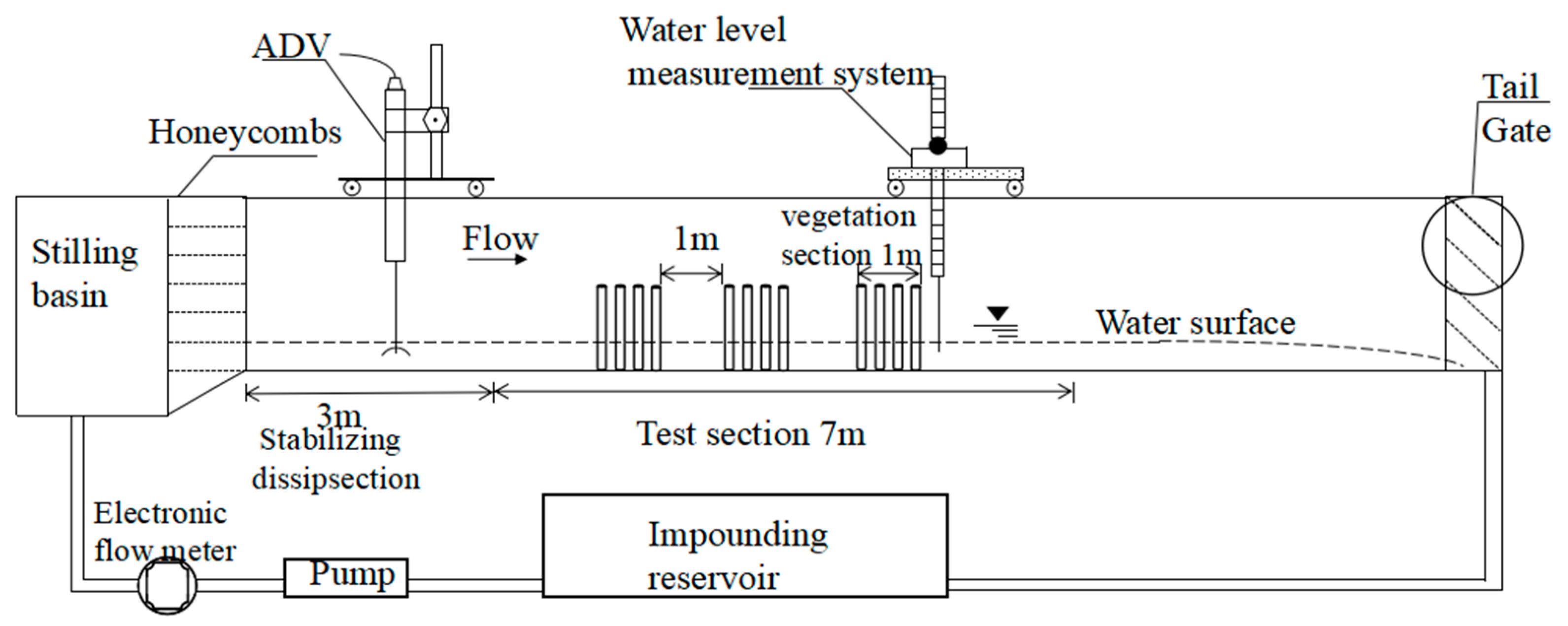
The experiment was conducted in a closed-loop open surface recirculating rectangular flume, with dimension of 12.5 m × 0.3 m × 0.3 m, at the Mechanism and Process of Gully Erosion Laboratory, the School of Soil and Water Conservation, Beijing Forestry University, China. A schematic sketch of the experimental setup and measuring instruments for test sections were shown in Figure 1. The water flow was pumped and controlled by a frequency water pump, and measured by an electromagnetic flow-meter installed in the entrance of the flume system, where a series of honeycombs was mounted to straighten the inflow and avoid large-scale disturbances. A tail gate was installed at the export of the flume to ensure the steady uniform state of the outflow. The experimental section was 3 m downstream from the entrance to establish a fully developed flow regime, and the length of the observation section was 7 m, where the simulated vegetation was fixed in a strip pattern. The Acoustic Doppler Velocimeter (ADV) and micrometer were adopted to observe the velocity and water depth, which could be moved in the longitudinal direction. Because positive and gentle slopes are commonly found in natural overland flows, the bed slope of the flume was set to a constant value of 1‰. This slope could ensure the steady flow state and avoid the breakage caused by steep slope [27]. The average flow rates were set to 0.8 L/s, 1.5 L/s, 1.9 L/s, 2.3 L/s, 2.9 L/s, 3.3 L/s, and 3.8 L/s to investigate the dynamic characteristics of overland flow with various inflow rates. The discharges were enveloped with a range within which the flow depth was constrained in a shallow overland flow condition, and the flow state could cover multiple zones [27,28]. The water temperature was monitored throughout the experimental process by a thermometer. The configurations were given in Section 2.2. In this experiment, the smallest breadth depth ratio was 5.7, under this kind of water depth state, the flow was quasi-two-dimensional flow [29], so that the effect of the side wall could be neglected.
2.2. Vegetation Material and Configurations
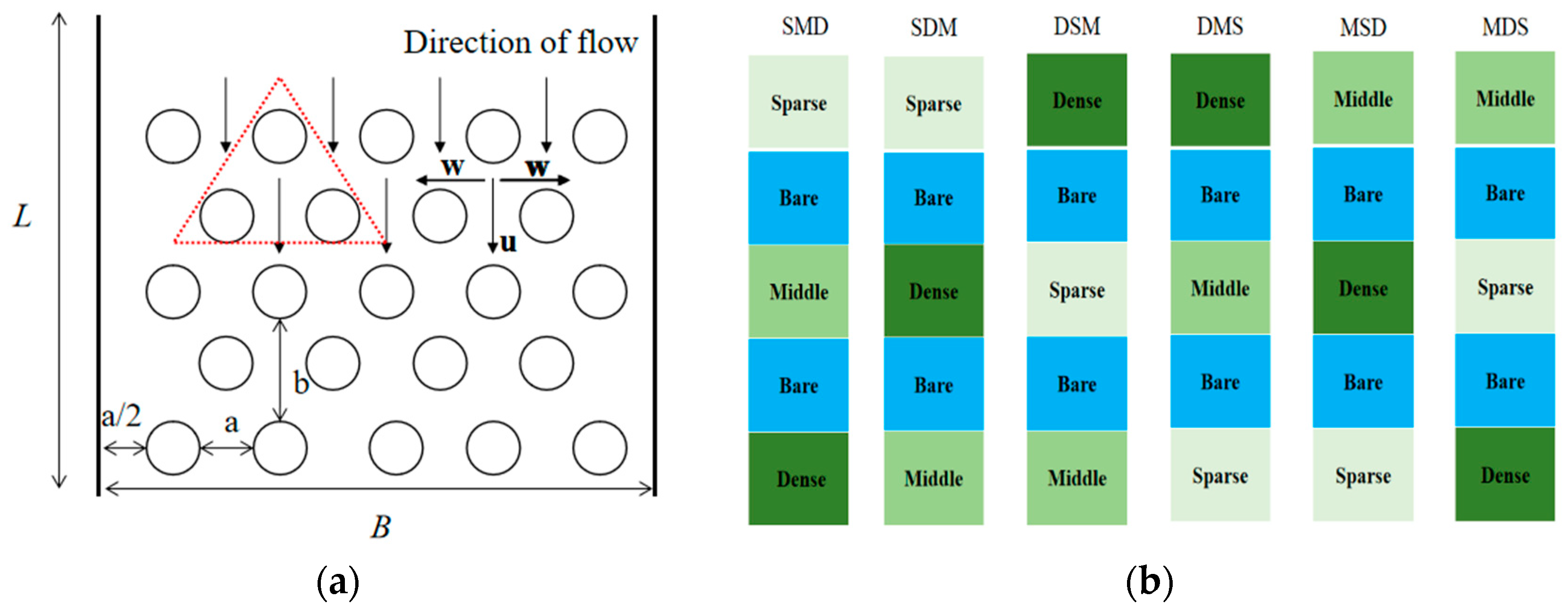
Artificial plants made of polyvinyl chloride (PVC) pipes with an outer diameter d = 1 cm and height hr = 10 cm were used in this study to simulate rigid unsubmerged vegetation. The cylinders were arranged in a staggered pattern to form regular triangles (Figure 2a). Three different vegetation densities (Sparse (1%), Middle (2%), and Dense (4%)) were selected, which were defined by the ratio of the bottom areas of all stems to that of the flume area for the vegetated section with the given equation:
where L is the length of the test section (1 m in this study), B is the flume width (30 cm in this study), a is the distance between two stems in the lateral direction (m), b is the distance between two stems in the longitudinal section (m), and d is the diameter of cylinder (m).
As the vegetated and non-vegetated testing areas were alternatively mounted in 1 m intervals and with 1 m vegetated sections, a total of six arrangements were oriented along the summit, backslope and footslope as shown in Figure 2b: Sparse-Middle-Dense (SMD); Sparse-Dense-Middle (SDM); Dense-Sparse-Middle (DSM); Dense-Middle-Sparse (DMS); Middle-Sparse-Dense (MSD); and Middle-Dense-Sparse (MDS). The main date of the experiments were shown in Table 1.
2.3. Locations of Flow Measurements
To obtain reliable and accurate results, the water depths were measured at three longitudinal sections in this experiment with 1 mm measuring accuracy. These longitudinal sections were located 15 cm, 7.5 cm, and 0 cm away from one side wall and named LS1, LS2, and LS3, respectively. On these longitudinal sections, measurement points were established at 25 cm intervals along the test section, with an increase in the number of observation points at the outflow section (S25, S26, and S27) (Figure 3a). In the direction of the vertical profile (Figure 3c), the flow velocities were measured every 0.4 cm by ADV from the bottom to the water surface (Figure 3c). Due to instrument limitations, flows within 2.5 cm from surface could not be detected. Note that the number of measurement points in each section differed, due to the differences in water depth. The ADV has three acoustic receivers and one acoustic transmitter, and it provides water velocity measurements in three directions: the longitudinal component (u), the transverse component (v), and the vertical component (w). In previous studies [30], the mean flow velocity stabilized when the measurement duration was greater than 45 s. Thus, the test time of the flow velocity measurement time was set to 60 s with a 6000 sampling number at 100 Hz, and the sampling volume was 7 × 10⁻² m3. The distance from the probe to the measurement point was 2.4 × 10⁻⁶ m. To ensure the quality of the measurement data, the signal-to-noise ratio of the measurements was maintained a 15 dB [31]. The average velocity at each point was calculated from the observations of 3000 samples. The observations were performed between two rows of simulated vegetation stems to eliminate the impact of acute changes in the simulated vegetation section as much as possible.
2.4. Parameter Determination
(1) Mean velocity
Mean velocity is an important hydrodynamic parameter, and it is also the major index indicating flow intensity. The mean flow velocity was calculated from the mean flow depth using the following equation:
where u is the mean flow velocity of a certain cross section, and h is the mean of the measured flow depths (m). In addition, the unit flow discharge (m3·s−1·m−1) is represented by , where is the flow discharge ().
(2) Flow-state indicator
When the flow is stable, the flow-state indicator can be calculated as follows [32]:
where m is the flow-state indicator, which indicates the magnitude of energy consumption, the larger the m, the more energy of the water flow is consumed by resistance; and k is a comprehensive index associated with the different arrangements, and it reflects the bed surface characteristics and flow viscosity. A larger interaction force of surface matter corresponds to a stronger effect of surface matter on the water flow across the slope.
(3) Reynolds number
The Re is a dimensionless number that is used to define flow regimes. The Re on vegetated slopes could be calculated using the following equation:
Bare slope:
Vegetated slope:
where the direct factor is the hydraulic radius (m), and P is the wetted perimeter. Equations (5) and (6) are for non-vegetated and vegetated slopes, respectively. In addition, m1 is the number of stems of each cross section, and v is the kinematic viscosity of clear water (cm2·s−1), which is calculated as v = 0.01775/(1 + 0.0337t + 0.000221t2), and t is the flow temperature (°C).
(4) Froude number
The mechanical definition of the Froude number (Fr) is the contrast relation between the inertial force and gravity, and it is the critical value characterizing the water flow pattern. A sub-critical flow occurs when Fr < 1, and super-critical flow occurs when Fr > 1. The Fr be calculated as follows:
where g is the acceleration of gravity.
(5) Total energy
The total energy for each longitudinal section can be calculated using the following energy equation:
In the present study, the channel bed at the end of vegetation section is considered as the datum plane; z is the vertical distance of the channel bed from the datum plane; and α is the correction factor, and it was equal to 1 in the present research.
(6) Darcy–Weisbach coefficient
The flow resistance in present study was calculated using the method of Hessel [33]. The resistance coefficient is calculated as follows:
where J is the hydraulic gradient. In this paper, the value of the hydraulic gradient was replaced by the sinusoidal value of the slope, which is 1‰.
(7) Manning coefficient
The Manning coefficient is related to the vegetation density and flow velocity. The general equation for the Manning coefficient is as follows:
where n is the Manning coefficient. This formula is applicable for non-vegetated conditions, and Noarayanan et al. [34] modified this equation for vegetated conditions using rigid tubes to mimic plants. The modified equation was also used in Li’s paper [35]:
where nveg is the Manning coefficient with vegetation only; uveg+wall is the velocity measured with vegetation section. uwall is the velocity measured without vegetation. uu(wall) is the upstream velocity measured without vegetation. ud(wall) is the downstream velocity measured without vegetation. hu(wall) is the depth of flow at the downstream location without vegetation, hd(wall) is the depth of flow at the downstream without vegetation. Hf(wall) is the head loss due to side and bottom wall; Sveg+wall is the energy slope in the presence of vegetation; Swall is the energy slope without vegetation.
(8) Turbulence intensity
The turbulence intensity was calculated using the following equations:
where is the total number of velocities obtained; , , and represent the stream-wise velocity, span-wise velocity and vertical velocity, respectively; and , , represent the mean velocities in the three directions.
(9) Reynolds stress number
To determine the effects of the different vegetation densities on the Reynolds stress profile, the Reynolds stress number (RSN) was calculated using the following equation:
3. Results and Discussion
3.1. Total Hydrodynamic Parameters under Different Vegetation Configurations
3.1.1. Flow Velocity and Flow State
Both the mean velocities u and Re increased with the increases of the flow discharge (0.01 < Pu < 0.05, 0.01 < PRe < 0.05, where Pu and PRe values are the significant levels of the Pettitt test) (Figure 4a,b). The u, Re, and Fr values on the bare slope were roughly twice as large as that on the vegetated slopes. In addition, a power relationship was observed between the u and flow discharge on both bare and vegetated slopes, according to the regression analysis (Table 2), and similar relationships have widely been reported in previous studies [36,37]. The Fr number and Darcy–Weisbach coefficient f on vegetated and non-vegetated slopes were quite different (Figure 4c,d). The flow on the bare slope was super-critical (Fr = 1.2) but sub-critical on vegetated slopes, which presented Fr values ranging from 0.4 to 0.6. The Fr ranked from lowest to highest was as follows: SMD < MSD < SDM < DSM < MDS < DMS. The smaller the Re and Fr were, the more stable the flow state would be, and the erosion on the underlying surface would be possibly smaller. Theoretically, during actual runoff process, the vegetation stems could potentially increase the infiltration and reduce the runoff and then weaken the soil erosion. As the observation was conducted under the same slope value (1‰), these results were reasonable and applicable for gentle slope.
To better describe the flow patterns, the flow-state indicator was calculated using Equation (3). As shown in Table 3, the m value of 0.4559 on the bare slope indicates that the flow energy was mainly kinetic energy. The m values on the vegetated slopes were comparably larger, with a ranking of SMD > MSD > SDM > DSM > MDS > DMS > Bare. The m values for all vegetated slopes were greater than 0.5, suggesting that the energy was dominantly consumed against flow resistance; moreover, energy that could be converted to kinetic energy was a supplementary component [33]. The k values showed no obvious variation pattern, which may because this value was influenced by multiple factors [38].
3.1.2. Darcy–Weisbach Friction Coefficient
In general, the f value for different vegetation patterns differed significantly (Figure 4d). For the six density arrangements, the f values were ranked as follows: SMD > MSD > SDM > DSM > MDS > DMS. This result indicated that the SMD pattern had the largest resistance coefficient. Our findings demonstrated that vegetation with greater density at the footslope position was more effective at reducing the dynamics of overland flow than the other configurations. The result was consistent with previous studies [39,40], which indicated that high vegetation densities at the footslope position were capable of resisting more accumulated momentum from the upslope areas. However, runoff flow at the footslope position were more likely to occur, due to the more significant changes in momentum coefficient [13].
3.1.3. Relationships between Re and f
A power law function between Re and f was found on the bare slope (Figure 5), which had been demonstrated in previous studies [41]. Separate regression equations for f versus Re for all vegetated slopes were derived and shown in Table 4. For vegetated slopes, only the f-Re relation of the DMS configuration exhibited a similar law as that of the bare slope. Figure 5 demonstrates that the curve of the resistance coefficient was almost parallel to the horizontal axis, and the f values changed indistinctly. Al Hamdan et al. [42] also found that f and Re did not show a consistent or single monotonic relationship on vegetated slopes, the variation in f with Re was much less pronounced, and the relationship between these two parameters became increasingly weaker. The overall result suggests that Re was not a consistent and unique predictor of hydraulic roughness on vegetated slopes.
3.2. Longitudinal Hydrodynamics under Different Vegetation Configurations
The features of hydrodynamic parameters along the flume were further investigated. As the regularity of all results for different inflow discharges were quite similar, we only enumerated one group of results at a constant discharge of 3.8 L/s.
3.2.1. Water Depth, Mean Velocity, and Total Energy
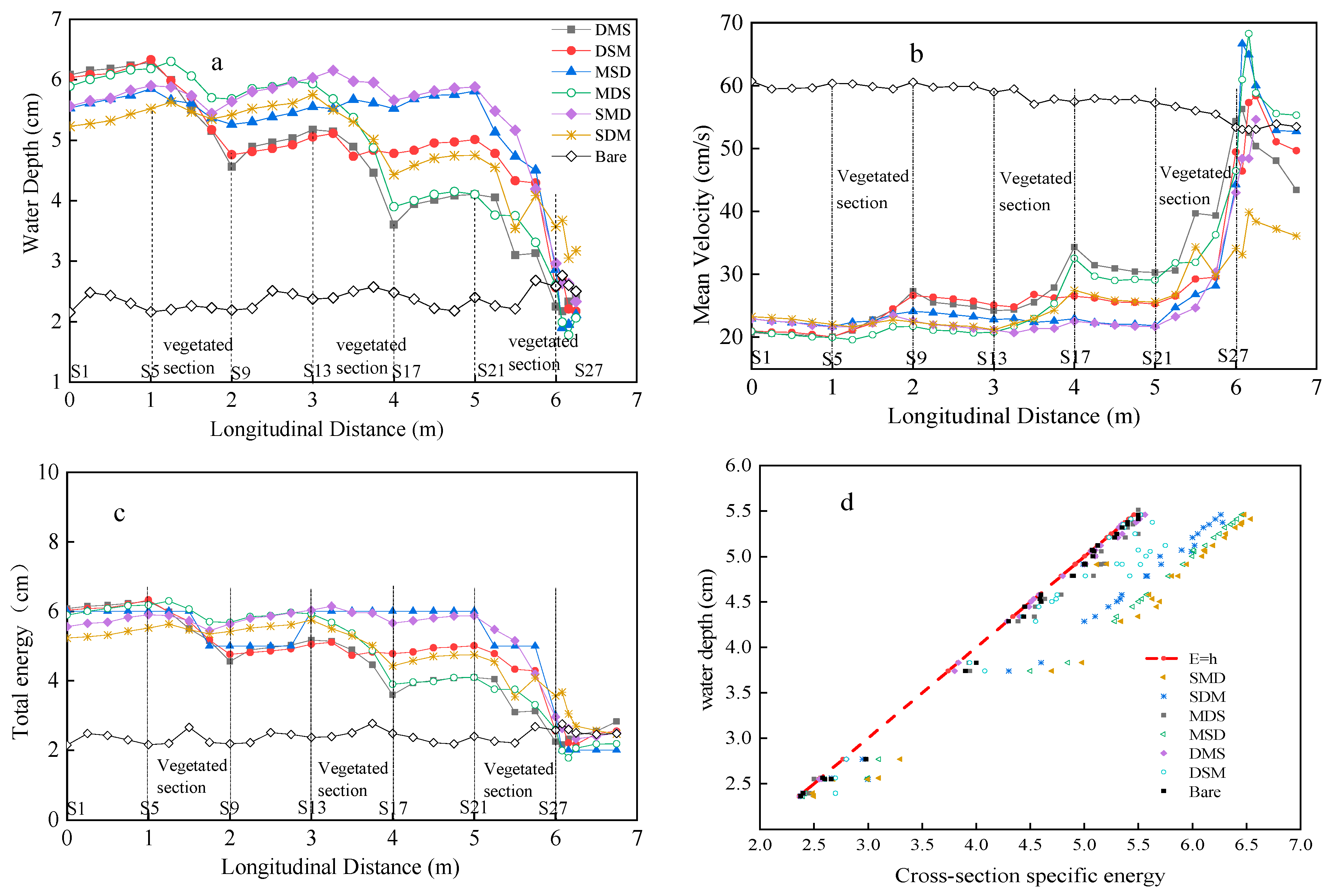
As shown in Figure 6a, the water depth h, which represented an average of the values of the three longitudinal sections, on the bare slope was generally lower than that on the vegetated slope. Zhang et al. [9] also found the same result. Throughout the tested sections, the difference of h between the starting and ending sections for the six vegetated configurations was ranked as SMD < MSD < SDM < DSM < MDS < DMS. This result indicated that a dense rearward arrangement led to a smaller change in h and to a better water-blocking effect in the test section. Furthermore, increasing and decreasing trends were found for the non-vegetated and vegetated sections, respectively, demonstrating a blocking effect before the vegetated area and rapid conveyance effect in the vegetated area. Accordingly, in each vegetation section, the h increased and reached its peak value nearly 0.25 m after entering the vegetated section, and it subsequently decreased. After the S27 cross section, the water depth sharply decreased, and h varied in the order of DMS < MDS < DSM < SDM < MSD < SMD. Because of the water blocking of the backside vegetation section, the water depth gradually increased before the vegetation section, and denser vegetation at the rear of the order corresponded to a better accumulation effect of vegetation on water blocking. Correspondingly, the u of the bare slope was generally larger than that of the vegetated slopes before section S27 (Figure 6b), and similar results were also found in previous studies [11,23]. The mean velocities on the vegetated slopes ranked from lowest to highest, as follows SMD < MSD < SDM < DSM < MDS < DMS. This result indicated that the dense rearward arrangement helped to reduce the mean velocity, which potentially reduced the distance and the amount of sediment transport [43]. Therefore, flow velocity was proved to be a dominating parameter in the research of slope hydrological processes, which would further affect soil erosion and sediment transportation [44,45]. Due to the reverse relationship between h and u (Equation (2)), decreasing and increasing trends were found at the vegetated and unvegetated sections, respectively.
The total energy (E) for each longitudinal location was calculated to evaluate the energy dissipating processes (Figure 6c). On the vegetated slopes, the E showed a fluctuating downward trend, whereas on the bare slopes, the E was mostly stable, and this parameter could be ranked as SMD > MSD > SDM > DSM > MDS > DMS > Bare. The decreasing trend on vegetated slopes indicated that the presence of plants enhanced the dissipation of the E. Prior to S27, the experimental arrangements could be ordered according to the fluctuating E value: SMD < MSD < SDM < DSM < MDS < DMS. For the vegetated and bare slopes, the E flow tended to converge at the end of S27, where the effect of vegetation on E disappeared.
The profiles of the E (Figure 6c) was consistent in terms of the tendency of the water surface profiles (Figure 6a). The cross-section specific energy curve (Figure 6d) demonstrated positive linear relationships between the specific energy and the water depth (Figure 6d), indicating subcritical flow states. In the experiment, a distance was observed between the cross section-specific energy and 1:1 line. The distance from the potential energy trend line (red line) represents the proportion of potential energy in the E. A greater deviation of the red line indicates a lower percentage of the potential. Therefore, Figure 6d showed that the primary component of E was potential energy, and that the proportion of potential energy was ranked as follows: SMD < MSD < SDM < DSM < MDS < DSM. Huang et al. [46] and Schutten et al. [47] reported that the cross-section-specific energy in rigid vegetation channels increased with the increasing of water depth, and it tended to be a straight line with a 45 degree angle to the horizontal level.
3.2.2. Reynolds Number and Froude Number
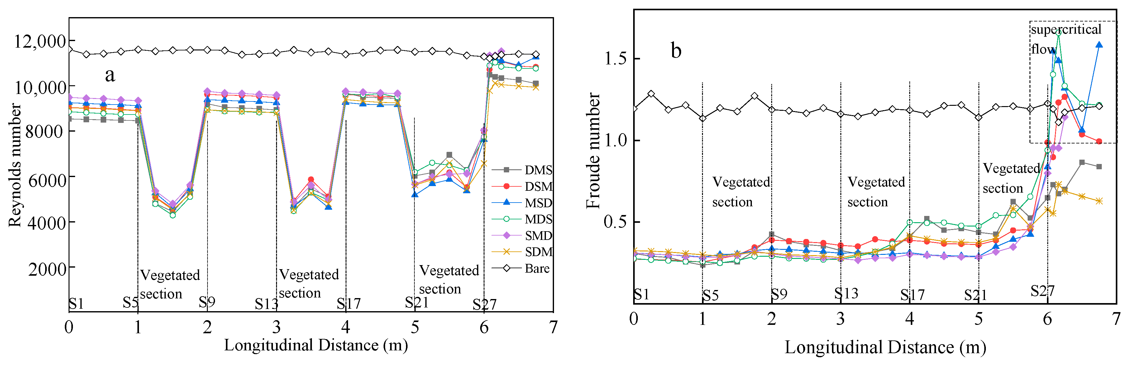
The Re values along the flow direction ranged from 4400 to 11,200, which corresponded to transitional and turbulent flow regimes (Figure 7a). Wang et al. [6] also found that overland flow began with transitional flow at the top of a given slope, and finished with turbulent flow on the bottom. The comparably smaller Re values on vegetated slopes than that of the bare slope indicated less intense turbulent characteristics. In addition, on vegetated slopes, the Re values at vegetated sections (4000–6000) were much smaller than those of nonvegetated sections (8000–10,000). Previous studies also found that the turbulent intensity would decrease further with the increase in vegetation coverage [18,48]. Moreover, Zhao et al. [23] found that increasing vegetation cover was crucial to reducing soil loss. A decrease in Re meant a decrease in the flow turbulence and erosion force, and it resulted in a further reduction of soil loss. Moreover, the Re increased sharply directly after the flow exited the vegetated sections, which was mainly because vegetation not only reduced the energy and dispersed runoff, but also increased the surface roughness. Thus, vegetation played an important role in delaying the flow velocity over slopes.
A significant difference was observed between the vegetated and non-vegetated slopes in terms of the Fr. As shown in Figure 7b, the Fr of the bare slope ranged from 0.98 to 1.35, while the Fr was less than 1 before S27 for the vegetated slope, suggesting that the vegetated slope under all experimental conditions showed subcritical flow. Most studies have demonstrated that the flow in a vegetated channel was subcritical, while supercritical flow along a vegetated surface was rare [49]. In our study, the Fr increased rapidly after S27, and the subcritical flow became supercritical. In this manner, it could be implied that the arrangement of vegetation density would affect the formation and the development of soil erosion processes along the slope, and the footslope would be more easily eroded due to the complexity of flow patterns. Therefore, the location of the outflow (S27) where the flow state rapidly changed should strengthen the protection.
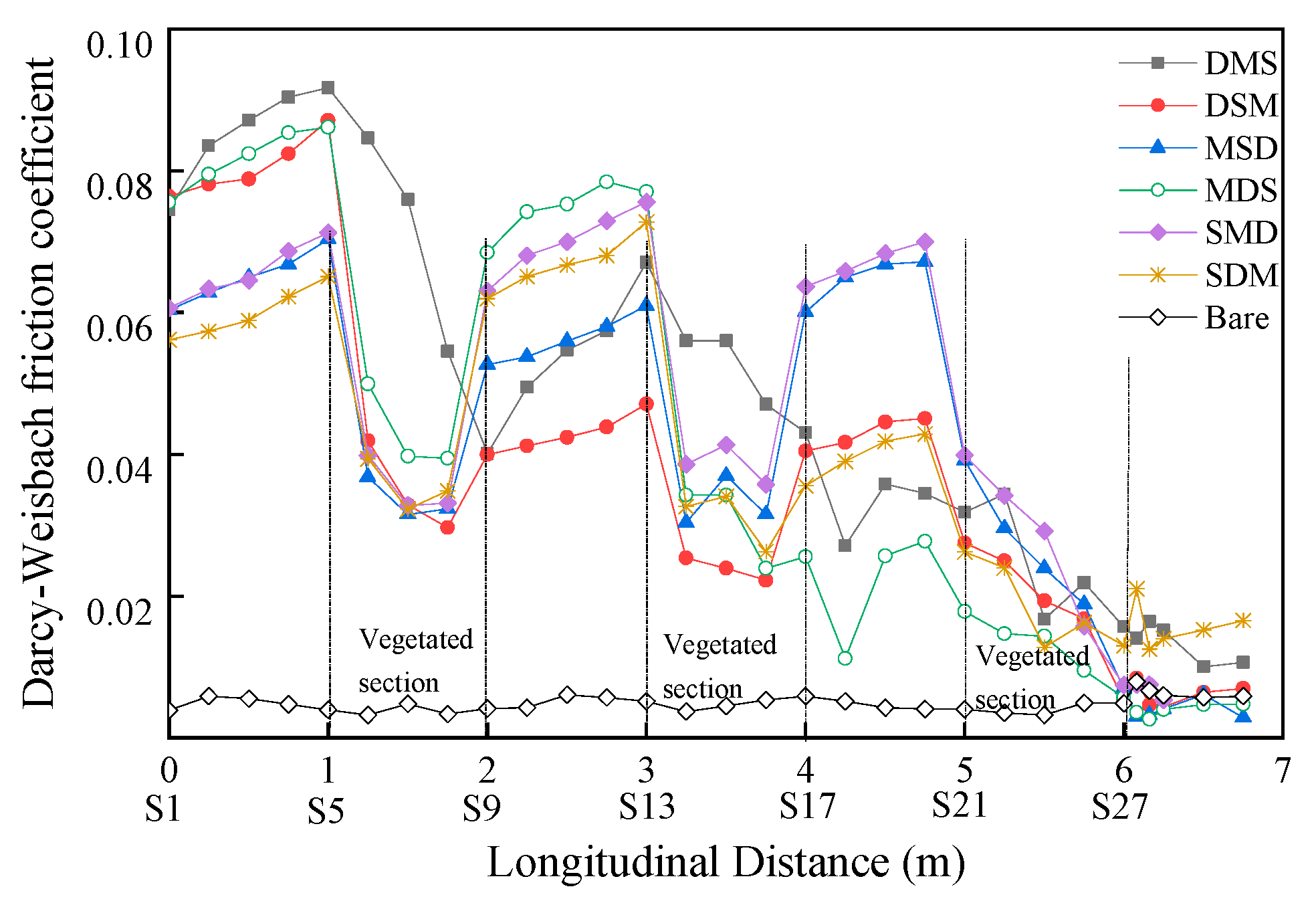
3.2.3. Darcy–Weisbach Friction Coefficient and Manning Coefficient
The f value exhibited a fluctuating downward trend ranging from 0.09 to 0.02 on vegetated slopes, and showed high values on non-vegetated sections and smaller values on vegetated sections. Meanwhile, f maintained a constant value of 0.0048 on the bare slope (Figure 8), and this value was two to 20 times smaller than that of the vegetated slopes, indicating that the presence of vegetation could significantly increase the resistance, such as the form resistance and wave resistance, which were the dominant elements in the vegetated section [50]. The f value decreased in the vegetation section, and gradually increased in the non-vegetation section. This was because in Equations (2) and (7), f was closely related to the variation of water depth. The presence of plants led to increasing water depth at the forepart and decreasing flow velocity. Specifically, the resistance was affected by the intervals: fDMS was highest at the first section (S1–S5), fMDS was highest at the second section (S9–S13), and fSMD was highest at the third section. These findings demonstrated that the regional resistance coefficient of the forepart of the vegetation was proportional to the density of the rear vegetation. Overall, increases in vegetation coverage were beneficial to the siltation of a large amount of sediment, and achieved the functions of soil and water conservation [51,52].
Because the Manning roughness coefficient is advantageous when comparing vegetated and non-vegetated conditions, the n values were derived by Equations (11)–(13) to compare the water-blocking effect of vegetation in different density arrangements (Table 5). For the same vegetation densities, the n values varied greatly in the different arrangements, which demonstrated that the location of the vegetation had a considerable impact on the water blocking effect of plants. The sum of the Manning coefficient for each arrangement ranked from the highest to the lowest was as follows: SMD > MSD > SDM > DSM > MDS > DMS. The n values of the footslopes were the largest ones among all arrangements, illustrating that the vegetation density at the footslope plays a key role in water resistance.
3.3. Vertical Dynamics at Typical Cross-Sections under the Optimal Configuration
As mentioned in Section 3.1 and Section 3.2, the SMD arrangement was much more effective in increasing the flow resistance, storing E, reducing erosion and turbidity, and maintaining a steady flow pattern. Therefore, the SMD pattern was taken as the optimal configuration, and the vertical dynamics and turbulent characteristics of this pattern at typical sections S2, S6, S10, S14, S18, and S22 (Figure 3a) were detected. Due to the limitations of ADV measurements, measurements could not be performed after S27, since the water flow was too shallow. Similar observations were found on bare slopes compared with vegetated slopes.
3.3.1. Velocity Profile
The dimensionless velocity profiles for the six sections were shown in Figure 9; in this term, represented the mean of stream-wise velocities at a certain point, and represented the average stream-wise velocity of the whole velocity profile. z/h was relative water depth, h was the water depth of each section, z was the depth of each measuring point. Under the SMD arrangement, we arranged the flow discharge as 3.8 L/s (maximum), the vertical velocity profiles of vegetated sections gradually approached the velocity profile of the bare slope on S6, S14, and S22, whereas the velocity profiles of non-vegetated sections gradually departed from the vertical velocity profile of the bare slope on S2, S10, and S18. Bennett et al. [53] carried out an experimental study on the change of velocity distribution caused by vegetation compression, and their results showed that vegetation can obviously reduce the velocity both inside and around the vegetation section, and the flow was compressed by vegetation but tended to easily cross the non-vegetated section.
All of the velocity profiles followed a power law only for z/h values greater than 0.2. The curve-fitting equations of vertical distribution profiles using data for z/h > 0.2 were shown in Table 6. Along the vertical plane, the velocity profile could be divided into three parts in the last section (S22): the first layer was 0–0.2 h, where the flow velocity increased rapidly. In this part, the low velocity area was near the bottom, and it could be approximately regarded as shear velocity [54]. The second layer was 0.2 h–0.4 h, where the velocity decreased because of disturbances to the vegetation stems, and the resistance and pressure gradient caused the transverse turbulence intensity of the plant to outweigh the vertical stress due to the disturbance of the plant. The third layer was 0.4 h–1 h, where the velocity increased rapidly until the top of the plant stem, which it stabilized. The third area represented the main area of turbulent exchange, where the balance of momentum was maintained, and changes in this section were mainly due to the sudden change of velocity at the top of the plant, which produced shear stress and led to turbulence. Chen et al. [55] also observed three layers based on the velocity distribution profile, which supported the idea that the flows in the region near the bed and at the top of the stems were very unstable, and led to the formation of coherent structures. Previous studies have found that sediment transport occurred in the range of 0–0.2 h [56]. Therefore, the last section, where the vertical velocity increased rapidly and was greater than that of bare flow, had the highest possibility of severe soil erosion. Except for section S22, the velocity profiles in other sections could be divided into two layers: the first layer was 0–0.2 h, which was mainly affected by the bottom layer, velocity gradient was generated by shear stress of the viscous sub-layer, it was equivalent to the first layer of the three layers and presented rapid increases in flow velocity. The second layer was above 0.2 h, and the velocity was almost stable. Thus, vegetation density had an obvious influence on the vertical velocity distribution, and a density threshold may have influenced the turbulence intensity distribution [57].
3.3.2. Reynolds Stress Number
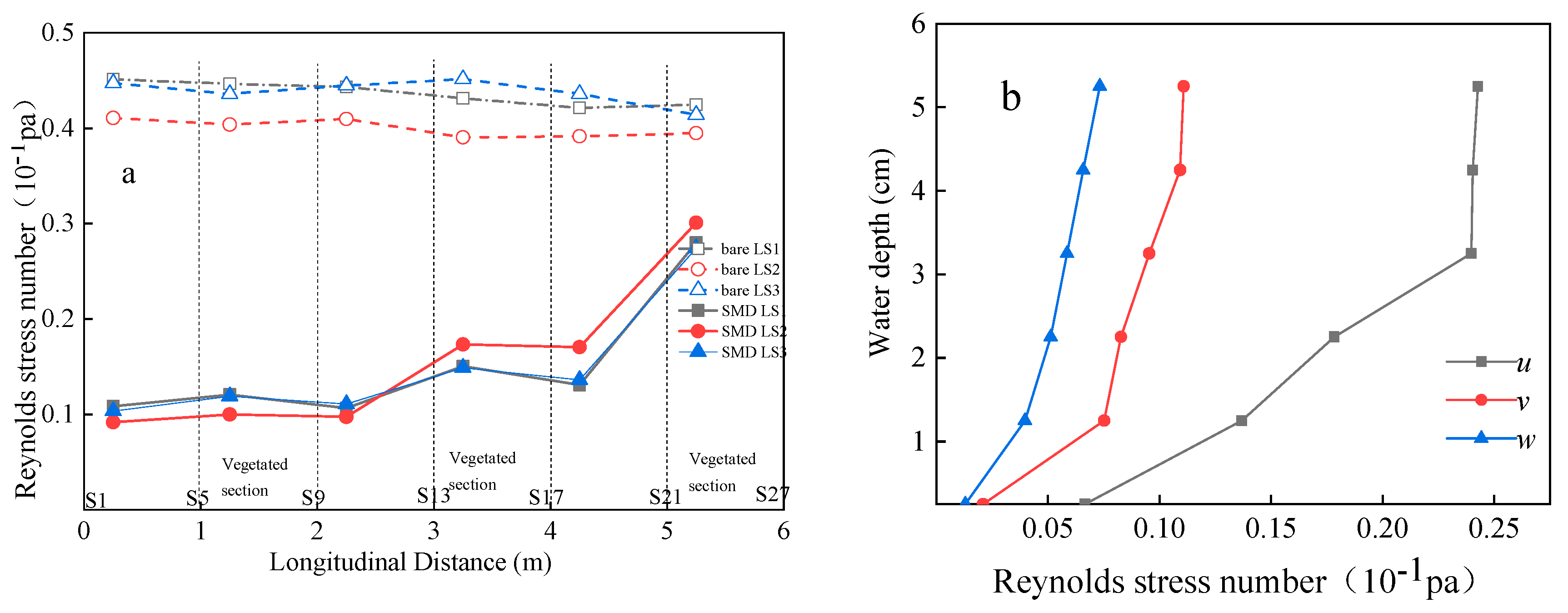
Blockage by aquatic vegetation could affect the turbulence structure in vegetated areas, even in s sparse population of rigid emergent vegetation [58]. The RSN for all three longitudinal sections at S2, S6, S10, S14, S18, and S22 were calculated for the SMD arrangement and bare slope (Figure 10a).
The RSNs on the bare slope were five times as large as those on the vegetated slope, and because they were not affected by any vegetation factors, they appeared to be more stable. By analyzing the significant level of differences between RSNs at different longitudinal sections LS1, LS2 and LS3 ( = 0.97), it could be deduced that the effect from the wall could be neglected. For the SDM arrangement, the RSN values were always higher near the beginning of the vegetation section. The RSNs of LS1, LS2, and LS3 decreased in the non-vegetation section, and increased in the vegetation section. The flow was less disturbed by vegetation before it entered the vegetation section, and the RSN presented obvious increases after entering the vegetation section; thus, the RSNs in the vegetation section increased as the vegetation density increased. Particularly, the RSNs in the last vegetation section were 2.5 times larger than that of the non-vegetation section, which may be caused by the horseshoe vortex [59] and the karman vortex [60] generated by the impediment of the vegetation stem. The presence of these vortices would successively cause the rise of turbulent kinetic energy [61]. Figure 10b exhibited the vertical depth distribution of RSN in different directions of LS1 at the last cross section of SMD arrangement, which basically changed in a consistent manner: as the water depth increased, the RSN initially increased and then decreased. The sequence of the three directions was longitudinal (u) > transverse (v) > vertical (w).
These results suggested that the presence of vegetation could effectively decrease the turbulent energy and RSNs than bare slope [55], which would efficiently decrease soil erosion by modifying the whole velocity profile and momentum distribution. Nevertheless, certain local locations, e.g., the footslope, were prone to be featured with more intensive turbulent intensities, and thus they accelerated the staring of the sediment load. Therefore, more measures should be taken into account for the protection of soil and water loss.
4. Conclusions
The hydrodynamics features of overland flow affected by emergent rigid vegetation with different density and location arrangements, i.e., SMD, SDM, DSM, DMS, MSD and MSD, were investigated in this study. A fixed flume experiment was conducted under seven different flow rates, and the hydrodynamic characteristics in multiple directions (traverse, longitudinal, and vertical) were highlighted based on the hydrodynamic parameters (v, h, Re, Fr, f, n, and E), turbulent intensity, and RSN. The main findings were as follows.
- (1)
- The variation laws of the total hydrodynamic parameters versus discharge on the vegetated slopes were quite similar to that of the bare slopes, although significant differences were observed in the v, Re, and Fr values, which were approximately two or three times larger than that of the bare slope, and the f value, which was approximately eight times as large as that of the bare slope. The relationship between the f and Re became much less pronounced on vegetated slopes, suggesting that the Re was not a unique predictor of hydraulic roughness on vegetated slopes. Among all the slope arrangements, the SMD presented the lowest velocity, RSN, and Fr, and the largest resistance and Manning coefficient values.
- (2)
- Longitudinally, the hydrodynamic parameters maintained constant values on bare slopes, but exhibited spatial variations on the vegetated slopes. The velocity and water depth of different cross sections demonstrated the blocking effect before vegetated areas, and a rapid conveyance effect in vegetation areas. Similarly, E and f exhibited fluctuating downward trends, with the potential energy accounting for the greatest impact. For all vegetated arrangements, the Re values of the vegetated sections were half the value of the non-vegetated sections, whereas the Fr number showed a sharp growth after the water flowed out of the tested section. Analyses of the Manning coefficient demonstrated that vegetation density at the footslope played a key role in water resistance. Among the different vegetation arrangements, the h, Re, E, and f values suggested that the dense rearward arrangement (SMD) was the optimal vegetation pattern for regulating flow conditions and reducing water and soil loss.
- (3)
- Vertically, the velocity distribution was affected by the presence of vegetation. The dimensionless velocity profile generally followed the power law only for z/h values greater than 0.2. Specifically, three layers were recognized in the velocity profiles at the outlet section, whereas two layers were observed for the other sections, indicating a threshold of density coverage that influenced the turbulence intensity. The comparably smaller RSNs on vegetated slopes compared with bare slopes further illustrated the positive effect of vegetation on reducing flow dynamics. Nevertheless, the higher velocity at the bottom layer and the larger RSN value at section S22, which featured dense vegetation, indicated that local scour was most likely to occur at the end of the outflow section. This finding could help identify the mechanisms underlying local soil erosion, and provide guidance for forest management and environmental protection.
Author Contributions
Conceptualization, Y.W. (Yuting Wang), H.Z; Methodology, Y.W. (Yuting Wang), H.Z.; Software, Y.W. (Yuting Wang); Validation, H.Z., P.Y. and Y.W. (Yunqin Wang); Formal Analysis, Y.W. (Yuting Wang); Investigation, Y.W. (Yuting Wang); Resources, Y.W. (Yuting Wang); Data Curation, Y.W. (Yuting Wang); Writing-Original Draft Preparation, Y.W. (Yuting Wang), H.Z. and P.Y.; Writing-Review & Editing, H.Z.; Visualization, Y.W. (Yuting Wang); Supervision, H.Z., Y.W. (Yunqin Wang); Project Administration, H.Z., Y.W. (Yunqin Wang); Funding Acquisition, H.Z., Y.W. (Yunqin Wang).
Funding
The research was supported by the National Key R&D Program of China (NO.2017YFC050450203, NO.2017YFC0505303), the National Natural Science Foundation of China (51309006, 41571276).
Acknowledgments
The authors sincerely thank the anonymous reviewers for their valuable suggestions in improving the manuscript.
Conflicts of Interest
The authors declare no conflict of interest.
Notation
| the distance between two stems in the lateral direction | |
| the distance between two stems in the longitudinal direction | |
| the flume width (30 cm in this study) | |
| the outer diameter of cylinder | |
| total energy | |
| Darcy–Weisbash coefficient | |
| Froude number | |
| the acceleration of gravity | |
| the water depth of each section | |
| the height of cylinder | |
| the depth of flow at the downstream location without vegetation | |
| the depth of flow at the downstream without vegetation | |
| the head loss due to side and bottom wall | |
| hydraulic gradient | |
| the comprehensive index associated with the different arrangements | |
| the length of the test section (1 m in this study) | |
| the number of stems of each cross section | |
| flow-state indicator | |
| Manning coefficient | |
| the Manning coefficient with vegetation only | |
| total number of velocities obtained | |
| witted perimeter | |
| significant value of the Reynolds number | |
| significant value of the mean velocity | |
| the significance levels of RSN | |
| flow discharge | |
| unit flow discharge | |
| hydraulic radius | |
| Reynolds number | |
| the energy slope in the presence of vegetation | |
| the energy slope without vegetation | |
| the flow temperature | |
| the mean flow velocity of a certain cross-section | |
| instantaneous stream-wise velocity at a certain point | |
| the velocity measured with vegetation section | |
| the velocity measured without vegetation | |
| the upstream velocity measured without vegetation | |
| the downstream velocity measured without vegetation | |
| the mean of stream-wise velocities at a certain point | |
| the kinematic viscosity of clear water | |
| instantaneous span-wise velocity at a certain point | |
| the mean of span-wise velocities at a certain point | |
| instantaneous vertical velocity at a certain point | |
| the mean of vertical velocities at a certain point | |
| the vertical distance of the channel bed from the datum plane | |
| the correction factor | |
| vegetation density |
References
- Luhar, M.; Rominger, J.; Nepf, H. Interaction between flow, transport and vegetation spatial structure. Environ. Fluid Mech. 2008, 8, 423. [Google Scholar] [CrossRef]
- Gabarrón-Galeote, M.A.; Martínez-Murillo, J.F.; Quesada, M.A.; Ruiz-Sinoga, J.D. Seasonal changes in the soil hydrological and erosive response depending on aspect, vegetation type and soil water repellency in different mediterranean microenvironments. Solid Earth 2013, 4, 497–509. [Google Scholar] [CrossRef]
- Lieskovský, J.; Kenderessy, P. Modelling the effect of vegetation cover and different tillage practices on soil erosion in vineyards: A case study in vrÁble (slovakia) using watem/sedem. Land Degrad. Dev. 2014, 25, 288–296. [Google Scholar] [CrossRef]
- Chen, H.; Zhang, X.; Abla, M.; Du, L.; Yan, R.; Ren, Q. Effects of vegetation and rainfall types on surface runoff and soil erosion on steep slopes on the Loess Plateau, China. CATENA 2018, 170, 141–149. [Google Scholar] [CrossRef]
- Zhang, X.; Li, P.; Li, Z.B.; Yu, G.Q.; Li, C. Effects of precipitation and different distributions of grass strips on runoff and sediment in the loess convex hillslope. CATENA 2018, 162, 130–140. [Google Scholar] [CrossRef]
- Wang, G.Y.; Sun, G.R.; Li, J.K.; Li, J. The experimental study of hydrodynamic characteristics of the overland flow on a slope with three-dimensional geomat. Res. Dev. Hydrodyn. 2018, 30, 153–159. [Google Scholar] [CrossRef]
- Nepf, H.; Ghisalberti, M. Flow and transport in channels with submerged vegetation. Acta Geophys. 2008, 56, 753–777. [Google Scholar] [CrossRef]
- Tang, H.; Tian, Z.; Yan, J.; Yuan, S. Determining drag coefficients and their application in modelling of turbulent flow with submerged vegetation. Adv. Water Resour. 2014, 69, 134–145. [Google Scholar] [CrossRef]
- Zhang, H.Y.; Wang, Z.Y.; Xu, W.G.; Dai, L.M. Effects of rigid unsubmerged vegetation on flow field structure and turbulent kinetic energy of gradually varied flow. River Res. Appl. 2015, 31, 1166–1175. [Google Scholar] [CrossRef]
- Abu-Zreig, M.; Rudra, R.P.; Lalonde, M.N. Experimental investigation of runoff reduction and sediment removal by vegetated filter strips. Hydrol. Process. 2010, 18, 2029–2037. [Google Scholar] [CrossRef]
- Zhang, G.; Liu, G.; Wang, G.; Wang, Y. Effects of patterned Artemisia capillaris on overland flow velocity under simulated rainfall. Hydrol. Process. 2012, 26, 3779–3787. [Google Scholar] [CrossRef]
- Fattet, M.; Fu, Y.; Ghestem, M.; Ma, W.; Foulonneau, M.; Nespoulous, J. Effects of vegetation type on soil resistance to erosion: Relationship between aggregate stability and shear strength. CATENA 2011, 87, 60–69. [Google Scholar] [CrossRef]
- Kubrak, E.; Kubrak, J.; Kiczko, A. Experimental investigation of kinetic energy and momentum coefficients in regular channels with stiff and flexible elements simulating submerged vegetation. Acta Geophys. 2015, 63, 1405–1422. [Google Scholar] [CrossRef]
- Termini, D. Experimental analysis of turbulence characteristics and flow conveyance effects in a vegetated channel. Geophys. Res. Abstr. 2009, 11, 5792. [Google Scholar]
- Ludwig, J.A.; Wilcox, B.P.; Breshears, D.D.; Tongway, D.J.; Imeson, A.C. Vegetation patches and runoff-erosion as interacting ecohydrological processes in semiarid landscapes. Ecology 2005, 86, 288–297. [Google Scholar] [CrossRef]
- Dunkerley, D.; Domelow, P.; Tooth, D. Frictional retardation of laminar flow by plant litter and surface stones on dryland surfaces: A laboratory study. Water Resour. Res. 2001, 37, 1417–1424. [Google Scholar] [CrossRef]
- Hamilton, B.M.; Selby, M.J. Hillslope materials and processes. Trans. Inst. Br. Geogr. 1993, 19, 505. [Google Scholar] [CrossRef]
- Pan, C.; Shangguan, Z. Runoff hydraulic characteristics and sediment generation in sloped grassplots under simulated rainfall conditions. J. Hydrol. 2006, 331, 178–185. [Google Scholar] [CrossRef]
- Ali, M.; Sterk, G.; Seeger, M.; Stroosnijder, L. Effect of flow discharge and median grain size on mean flow velocity under overland flow. J. Hydrol. 2012, 452–453, 150–160. [Google Scholar] [CrossRef]
- Fu, W.; Huang, M.; Gallichand, J.; Shao, M. Optimization of plant coverage in relation to water balance in the loess plateau of China. Food Sci. Biotechnol. 2016, 25, 53–62. [Google Scholar] [CrossRef]
- Zhou, J.; Fu, B.; Gao, G.; Lü, Y.; Liu, Y.; Nan, L. Effects of precipitation and restoration vegetation on soil erosion in a semi-arid environment in the Loess Plateau, China. CATENA 2016, 137, 1–11. [Google Scholar] [CrossRef] [Green Version]
- Righetti, M. Flow analysis in a channel with flexible vegetation using double-averaging method. Acta Geophys. 2008, 56, 801–823. [Google Scholar] [CrossRef] [Green Version]
- Zhao, C.; Gao, J.; Zhang, M.; Wang, F.; Zhang, T. Sediment deposition and overland flow hydraulics in simulated vegetative filter strips under varying vegetation covers. Hydrol. Process. 2016, 30, 163–175. [Google Scholar] [CrossRef]
- Berhe, A.A.; Harden, J.W.; Torn, M.S.; Harte, J. Linking soil organic matter dynamics and erosion-induced terrestrial carbon sequestration at different landform positions. J. Geophys. Res. Biogeosci. 2015, 13, 4647–4664. [Google Scholar] [CrossRef]
- Rey, F. Effectiveness of vegetation barriers for marly sediment trapping. Earth Surf. Process. Landf. 2010, 29, 1161–1169. [Google Scholar] [CrossRef]
- Ding, W.; Mian, L.I. Effects of grass coverage and distribution patterns on erosion and overland flow hydraulic characteristics. Environ. Earth Sci. 2016, 75, 477. [Google Scholar] [CrossRef]
- Mujtaba, B.; de Lima, J.L. Laboratory testing of a new thermal tracer for infrared-based PTV technique for shallow overland flows. CATENA 2018, 169, 69–79. [Google Scholar] [CrossRef]
- Järvelä, J. Flow resistance of flexible and stiff vegetation: A flume study with natural plants. J. Hydrol. 2002, 269, 44–54. [Google Scholar] [CrossRef]
- Nezu, I. Open-channel flow turbulence and its research prospect in the 21st century. J. Hydraul. Eng. 2005, 131, 229–246. [Google Scholar] [CrossRef]
- Jing, Y.; Zhang, H.; Wang, Z.; Xu, W.; Ji, C.; Zhang, H. The Change of Relative Turbulence Intensity within the Reed Population. In Proceedings of the ASME 2010 International Mechanical Engineering Congress and Exposition, Vancouver, BC, Canada, 12–18 November 2010; pp. 397–401. [Google Scholar]
- Yılmazer, D.; Ozan, A.Y.; Cihan, K. Flow Characteristics in the Wake Region of a Finite-Length Vegetation Patch in a Partly Vegetated Channel. Water 2018, 10, 459. [Google Scholar] [CrossRef]
- Horton, R.E. Erosional development of streams and their drainage basins; hydrophysical approach to quantitative morphology. J. Jpn. For. Soc. 1945, 56, 275–370. [Google Scholar] [CrossRef]
- Hessel, R.; Jetten, V.; Zhang, G. Estimating manning’s n for steep slopes. CATENA 2003, 54, 77–91. [Google Scholar] [CrossRef]
- Noarayanan, L.; Murali, K.; Sundar, V. Manning’s ‘n’ co-efficient for flexible emergent vegetation in tandem configuration. J. Hydro-Environ. Res. 2012, 6, 51–62. [Google Scholar] [CrossRef]
- Li, Y.; Wang, Y.; Anim, D.O.; Tang, C.; Du, W.; Ni, L. Flow characteristics in different densities of submerged flexible vegetation from an open-channel flume study of artificial plants. Geomorphology 2014, 204, 314–324. [Google Scholar] [CrossRef]
- Zhou, S.M.; Lei, T.W.; Warrington, D.N.; Lei, Q.X.; Zhang, M.L. Does watershed size affect simple mathematical relationships between flow velocity and discharge rate at watershed outlets on the Loess Plateau of China. J. Hydrol. 2012, 444–445, 1–9. [Google Scholar] [CrossRef]
- Abrahams, A.D.; Li, G.; Parsons, A.J. Rill hydraulics on a semiarid hillslope, southern Arizona. Earth Surf. Process. Landf. 2015, 21, 35–47. [Google Scholar] [CrossRef]
- Richardson, J.R.; Julien, P.Y. Suitability of simplified overland flow equations. Water Resour. Res. 1994, 30, 665–671. [Google Scholar] [CrossRef]
- Gong, J.; Chen, L.D.; Fu, B.J.; Wei, W. Integrated effects of slope aspect and land use on soil nutrients in a small catchment in a hilly loess area, China. Int. J. Sustain. Dev. World Ecol. 2007, 14, 307–316. [Google Scholar] [CrossRef]
- Jackson, N.A.; Wallace, J.S.; Ong, C.K. Tree pruning as a means of controlling water use in an agroforestry system in Kenya. For. Ecol. Manag. 2000, 126, 133–148. [Google Scholar] [CrossRef]
- Takken, I.; Govers’, G. Hydraulics of interrill overland flow on rough, bare soil surfaces. Earth Surf. Process. Landf. 2015, 25, 1387–1402. [Google Scholar] [CrossRef]
- Al-Hamdan, O.Z.; Pierson, F.B., Jr.; Nearing, M.A.; Stone, J.J.; Williams, C.J.; Moffet, C.A.; Kormos, P.R.; Boll, J.; Weltz, M.A. Characteristics of concentrated flow hydraulics for rangeland ecosystems: Implications for hydrologic modeling. Earth Surf. Process. Landf. 2012, 37, 157–168. [Google Scholar] [CrossRef]
- Spaan, W.P.; Sikking, A.F.S.; Hoogmoed, W.B. Vegetation barrier and tillage effects on runoff and sediment in an alley crop system on a Luvisol in Burkina Faso. Soil Tillage Res. 2005, 83, 194–203. [Google Scholar] [CrossRef]
- Ban, Y.; Lei, T.; Gao, Y.; Qu, L. Effect of stone content on water flow velocity over loess slope. J. Hydrol. 2017, 554, 792–799. [Google Scholar] [CrossRef]
- Nadal-Romero, E.; Lasanta, T.; García-Ruiz, J.M. Runoff and sediment yield from land under various uses in a Mediterranean mountain area: Long-term results from an experimental station. Earth Surf. Process. Landf. 2013, 38, 346–355. [Google Scholar] [CrossRef]
- Huang, B.S.; Lai, G.W.; Qiu, J.; Lin, S.Z. Hydraulics of compound channel with vegetated floodplains. Res. Dev. Hydrodyn. 2002, 14, 23–28. [Google Scholar]
- Schutten, J.; Davy, A.J. Predicting the hydraulic forces on submerged macrophytes from current velocity, biomass and morphology. Oecologia 2000, 123, 445–452. [Google Scholar] [CrossRef] [PubMed]
- Wu, S.; Wu, P.; Feng, H.; Merkley, G.P. Effects of alfalfa coverage on runoff, erosion and hydraulic characteristics of overland flow on loess slope plots. Front. Environ. Sci. Eng. China 2011, 5, 76–83. [Google Scholar] [CrossRef]
- Kothyari, U.C.; Kenjirou, H.; Haruyuki, H. Drag coefficient of unsubmerged rigid vegetation stems in open channel flows. J. Hydraul. Res. 2009, 47, 691–699. [Google Scholar] [CrossRef]
- Hu, S.; Abrahams, A.D. Partitioning resistance to overland flow on rough mobile beds. Earth Surf. Process. Landf. 2006, 31, 1280–1291. [Google Scholar] [CrossRef]
- Xu, W.G.; Zhang, H.Y.; Wang, Z.Y.; Huang, W.P. A study of manning coefficient related with vegetation density along the vegetated channel. Appl. Mech. Mater. 2012, 212–213, 744–747. [Google Scholar] [CrossRef]
- Panigrahi, K.; Khatua, K.K. Analysis of different roughness coefficients’ variation in an open channel with vegetation. Ther. Adv. Respir. Dis. 2015, 9, 27–33. [Google Scholar]
- Bennett, S.J.; Pirim, T.; Barkdoll, B.D. Using simulated emergent vegetation to alter stream flow direction within a straight experimental channel. Geomorphology 2002, 44, 115–126. [Google Scholar] [CrossRef]
- Hopkinson, L.C.; Walburn, C.Z. Near-boundary velocity and turbulence indepth-varying stream flows. Environ. Fluid Mech. 2015, 16, 559–574. [Google Scholar] [CrossRef]
- Chen, S.C.; Kuo, Y.M.; Li, Y.H. Flow characteristics within different configurations of submerged flexible vegetation. J. Hydrol. 2011, 398, 124–134. [Google Scholar] [CrossRef]
- Fu, X.; Wang, G.; Shao, X. Vertical dispersion of fine and coarse sediments in turbulent open-channel flows. J. Hydraul. Eng. 2005, 131, 877–888. [Google Scholar] [CrossRef]
- Huai, W.X.; Zeng, Y.H.; Xu, Z.G.; Yang, Z.H. Three-layer model for vertical velocity distribution in open channel flow with submerged rigid vegetation. Adv. Water Resour. 2009, 32, 487–492. [Google Scholar] [CrossRef]
- Nepf, H.M. Drag, turbulence, and diffusion in flow through emergent vegetation. Water Resour. Res. 1999, 35, 1985–1986. [Google Scholar] [CrossRef]
- Sahin, B.; Ozturk, N.A.; Akilli, H. Horseshoe vortex system in the vicinity of the vertical cylinder mounted on a flat plate. Flow Meas. Instrum. 2007, 18, 57–68. [Google Scholar] [CrossRef]
- Atrah, A.; Ab-Rahman, M.; Salleh, H.; Nuawi, M.; Nor, M.M.; Jamaludin, N. Karman vortex creation using cylinder for flutter energy harvester device. Micromachines 2017, 8, 227. [Google Scholar] [CrossRef] [PubMed]
- Li, J.; Qi, M.; Fuhrman, D.R.; Chen, Q. Influence of turbulent horseshoe vortex and associated bed shear stress on sediment transport in front of a cylinder. Exp. Therm. Fluid Sci. 2018, 97, 444–457. [Google Scholar] [CrossRef]
Figure 1.
Schematic of the experimental setup (side view).

Figure 2.
Vegetation configurations: (a) Vegetation distribution in a staggered pattern; (b) Density configurations in at the summit, backslope and footslope.
Figure 2.
Vegetation configurations: (a) Vegetation distribution in a staggered pattern; (b) Density configurations in at the summit, backslope and footslope.

Figure 3.
Locations of measurement points: (a) Measured points along the flow direction in plan view; (b) Artificial plants and measuring instruments; (c) Measurement points along the water depth.
Figure 3.
Locations of measurement points: (a) Measured points along the flow direction in plan view; (b) Artificial plants and measuring instruments; (c) Measurement points along the water depth.

Figure 4.
Variations in the (a) mean velocity, (b) Reynolds number, (c) Froude number and (d) Darcy–Weisbach coefficient f with different flow discharges.
Figure 4.
Variations in the (a) mean velocity, (b) Reynolds number, (c) Froude number and (d) Darcy–Weisbach coefficient f with different flow discharges.

Figure 5.
Relationship between the Darcy–Weisbach friction coefficients and Reynolds numbers.

Figure 6.
Longitudinal variations in the (a) water depth, (b) mean velocity, and (c) total energy in the longitudinal direction, and (d) relationships between the cross-section-specific energy and water depth for all vegetation configurations.
Figure 6.
Longitudinal variations in the (a) water depth, (b) mean velocity, and (c) total energy in the longitudinal direction, and (d) relationships between the cross-section-specific energy and water depth for all vegetation configurations.

Figure 7.
Variations in the (a) Reynolds number and (b) the Froude number in the longitudinal direction.
Figure 7.
Variations in the (a) Reynolds number and (b) the Froude number in the longitudinal direction.

Figure 8.
Variation of the Darcy–Weisbach friction coefficients in the longitudinal direction.

Figure 9.
The vertical flow velocity distribution related to the relative water depth at different positions.
Figure 9.
The vertical flow velocity distribution related to the relative water depth at different positions.

Figure 10.
(a) Longitudinal variation of RSN values for the vegetated SMD arrangement slope and bare slope. (b) Relationship between the water depth and RSNs in different directions.
Figure 10.
(a) Longitudinal variation of RSN values for the vegetated SMD arrangement slope and bare slope. (b) Relationship between the water depth and RSNs in different directions.


Table 1.
Main data of the experiments.
| Configurations | Q (L/s) | H (cm) | R (cm) | V (cm2·s−1) |
|---|---|---|---|---|
| Bare | 1.12 | 1.20 | 1.03 | 0.009 |
| 1.75 | 1.36 | 1.18 | 0.009 | |
| 2.07 | 1.56 | 1.32 | 0.009 | |
| 2.60 | 1.82 | 1.50 | 0.009 | |
| 3.12 | 2.03 | 1.63 | 0.009 | |
| 3.52 | 2.10 | 1.76 | 0.009 | |
| 3.98 | 2.40 | 1.86 | 0.009 | |
| SMD | 1.05 | 0.70 | 1.61 | 0.009 |
| 1.65 | 2.10 | 2.08 | 0.009 | |
| 2.00 | 2.84 | 2.27 | 0.009 | |
| 2.43 | 3.31 | 2.56 | 0.009 | |
| 2.95 | 4.12 | 2.77 | 0.009 | |
| 3.4 | 4.59 | 3.04 | 0.009 | |
| 3.82 | 4.83 | 3.17 | 0.009 | |
| MSD | 0.38 | 2.04 | 0.65 | 0.01 |
| 1.13 | 2.85 | 1.61 | 0.01 | |
| 1.75 | 3.21 | 2.10 | 0.01 | |
| 2.07 | 3.83 | 2.35 | 0.01 | |
| 2.90 | 4.31 | 2.65 | 0.01 | |
| 3.40 | 4.92 | 2.88 | 0.01 | |
| 3.80 | 5.26 | 2.98 | 0.01 | |
| SDM | 0.73 | 2.04 | 1.80 | 0.01 |
| 1.42 | 2.24 | 1.82 | 0.01 | |
| 1.78 | 2.66 | 1.95 | 0.01 | |
| 2.30 | 3.16 | 2.23 | 0.01 | |
| 2.78 | 3.72 | 2.51 | 0.01 | |
| 3.22 | 4.17 | 2.71 | 0.01 | |
| 3.65 | 4.75 | 3.02 | 0.01 | |
| DSM | 0.55 | 1.40 | 1.20 | 0.009 |
| 1.3 | 2.12 | 1.66 | 0.009 | |
| 1.85 | 2.73 | 2.03 | 0.009 | |
| 2.15 | 2.84 | 2.20 | 0.009 | |
| 2.65 | 3.61 | 2.48 | 0.009 | |
| 3.15 | 4.06 | 2.69 | 0.009 | |
| 3.80 | 4.64 | 2.94 | 0.009 | |
| MDS | 0.90 | 1.69 | 1.38 | 0.01 |
| 1.56 | 2.39 | 1.80 | 0.01 | |
| 1.80 | 2.85 | 2.27 | 0.01 | |
| 2.30 | 3.24 | 2.40 | 0.01 | |
| 2.85 | 3.78 | 2.53 | 0.01 | |
| 3.30 | 4.23 | 2.73 | 0.01 | |
| 3.70 | 4.51 | 2.85 | 0.01 | |
| DMS | 0.8 | 1.67 | 1.38 | 0.009 |
| 1.5 | 2.50 | 1.88 | 0.009 | |
| 1.8 | 2.83 | 2.09 | 0.009 | |
| 2.3 | 3.30 | 2.30 | 0.009 | |
| 2.8 | 3.70 | 2.51 | 0.009 | |
| 3.3 | 4.10 | 2.71 | 0.009 | |
| 3.6 | 4.37 | 2.84 | 0.009 |
Table 2.
Relationship between the mean velocity and flow discharge.
| Configurations | Regression Equation | R2 |
|---|---|---|
| Bare | 0.9794 | |
| SMD | 0.9838 | |
| MSD | 0.9401 | |
| SDM | 0.9794 | |
| DSM | 0.9922 | |
| MDS | 0.9533 | |
| DMS | 0.9713 |
Table 3.
Values of the flow-state indicator m and k in the different experimental groups.
| Arrangement | Regression Equation | R2 | m | k |
|---|---|---|---|---|
| Bare | 0.9995 | 0.4559 | 0.1508 | |
| SMD | 0.9906 | 0.4392 | 0.0895 | |
| MSD | 0.9985 | 0.7384 | 0.1474 | |
| SDM | 0.802 | 0.467 | 0.4441 | |
| DSM | 0.9922 | 0.6231 | 0.2144 | |
| MDS | 0.9948 | 0.679 | 0.1707 | |
| DMS | 0.9995 | 0.6363 | 0.2065 |
Table 4.
Regression functions of the Darcy–Weisbach friction coefficients (f) and Reynolds numbers (Re) for each experimental arrangement.
Table 4.
Regression functions of the Darcy–Weisbach friction coefficients (f) and Reynolds numbers (Re) for each experimental arrangement.
| Underlying Surface | Function | R2 |
|---|---|---|
| Bare | 0.98 | |
| SMD | 0.16 | |
| MSD | 0.70 | |
| SDM | 0.40 | |
| DSM | 0.81 | |
| MDS | 0.25 | |
| DMS | 0.97 |
Table 5.
Manning coefficients for different density arrangement patterns.
| Density | SMD | SDM | MSD | MDS | DSM | DMS |
|---|---|---|---|---|---|---|
| 1% | 4.2 | 3.98 | 3.82 | 8.68 (foot) | 2.72 | 8.49 (foot) |
| 2% | 5.33 | 8.56 (foot) | 5.24 | 3.01 | 10.35(foot) | 3.72 |
| 4% | 12.43 (foot) | 6.46 | 11.88 (foot) | 5.31 | 4.93 | 3.31 |
| SUM | 21.96 | 19 | 20.94 | 17 | 18 | 15.52 |
Table 6.
The curve fitting equations of vertical distribution profiles.
| Position | Equation | R2 |
|---|---|---|
| Bare | 0.96 | |
| S2 | 0.82 | |
| S6 | 0.87 | |
| S10 | 0.88 | |
| S14 | 0.94 | |
| S18 | 0.90 | |
| S22 | 0.80 |
© 2018 by the authors. Licensee MDPI, Basel, Switzerland. This article is an open access article distributed under the terms and conditions of the Creative Commons Attribution (CC BY) license (http://creativecommons.org/licenses/by/4.0/).
Share and Cite
MDPI and ACS Style
Wang, Y.; Zhang, H.; Yang, P.; Wang, Y. Experimental Study of Overland Flow through Rigid Emergent Vegetation with Different Densities and Location Arrangements. Water 2018, 10, 1638. https://doi.org/10.3390/w10111638
AMA Style
Wang Y, Zhang H, Yang P, Wang Y. Experimental Study of Overland Flow through Rigid Emergent Vegetation with Different Densities and Location Arrangements. Water. 2018; 10(11):1638. https://doi.org/10.3390/w10111638
Chicago/Turabian StyleWang, Yuting, Huilan Zhang, Pingping Yang, and Yunqi Wang. 2018. "Experimental Study of Overland Flow through Rigid Emergent Vegetation with Different Densities and Location Arrangements" Water 10, no. 11: 1638. https://doi.org/10.3390/w10111638
Note that from the first issue of 2016, this journal uses article numbers instead of page numbers. See further details here.