Affordability of Decentralized Wastewater Systems: A Case Study in Integrated Planning from INDIA
by
Norbert Brunner
1, 
Markus Starkl
2,*,
Absar A. Kazmi
3,
Alvaro Real
4,
Nitin Jain
5 and
Vijay Mishra
1 1
Centre for Environmental Management and Decision Support (CEMDS), 1180 Vienna, Austria
2
University of Natural Resources and Life Sciences (BOKU),1180 Vienna, Austria
3
Indian Institute of Technology Roorkee (IITR), Roorkee, Uttarakhand 247667, India
4
Fundación Centro de las Nuevas Tecnologías del Agua (CENTA), 41820 Sevilla, Spain
5
Centre for Environmental Management and Decision Support (CEMDS) Development GmbH, 1190 Vienna, Austria
*
Author to whom correspondence should be addressed.
Water 2018, 10(11), 1644; https://doi.org/10.3390/w10111644
Submission received: 10 October 2018
/
Revised: 7 November 2018
/
Accepted: 10 November 2018
/
Published: 13 November 2018
(This article belongs to the Section Wastewater Treatment and Reuse)
Abstract
:Based on experiences about the planning of decentralized wastewater treatment systems for slums of two rural towns in India, the paper asks to what extent affordability for the future users may impede the realization of other sustainability goals. The planning aimed at ensuring economic, social, and environmental sustainability. To this end the planning process promoted the participation of stakeholders and it was supplemented by an in-depth analysis (using novel methods) of the socio-economic situation of the future users. In particular, an approach towards estimating willingness to pay from small samples was developed. Taking all this information into account, planning identified a well-established technology that it is inexpensive, robust, and easy to maintain. The experiences of this planning process may generalize to other developing countries seeking socially acceptable low cost solutions with reasonable pollution reduction for resolving the sanitation crisis.
1. Introduction
The United Nations’ Sustainable Development Goal No. 6 asks governments to ‘ensure access to water and sanitation for all’ [1]. In developing countries adequate sanitation remains a challenge and it has been suggested that ‘the progress made thus far on water and sanitation concerns cases of what might be called low-hanging fruit—i.e., those issues that are less challenging to address’ [2], because the policy goal of cost recovery from the users [3,4] may have excluded the very poor from improvements [5]. For, ‘although, for sustainable development, it is necessary to include a wide range of criteria (such as, environmental, technical, hygienic, and socio-cultural parameters) in the decision process, in most developing countries, economy is the most important criterion’ [6]. This criterion becomes even more important for the planning of sanitation improvements for slums, where the poverty of the future users may become a main barrier for cost recovery and thus for financial sustainability [7].
The paper asks, if a focus of planning on decentralized systems may facilitate the consideration of sustainability issues in a cost-dominated environment, as is suggested in literature [8]. It is based on a case study from slums in India, where policies are favorable towards decentralized systems [9]. For decentralized systems, the combined wastewater from a cluster of individual households is collected in sewers and treated close to the sources [10,11]. In developing countries decentralized systems have been identified as a cost-effective approach for rural towns [12], where additional ecological benefits may be realized; e.g., through water recycling for irrigation [13]. Also, in industrialized countries there are many positive experiences, where decentralized systems supported the policy goal of a ‘circular economy’, as they allowed for the implementation of innovative water recycling solutions [14] and supported the movement towards ‘green chemistry’ [15,16]. Another advantage was the flexibility and resilience of planning [17]. Thus, municipalities can respond step by step to the most pressing sanitation needs; this allows them to remain within the limits of their budgets.
For the case study, poverty was a main constraint for the planning. To what extent could the policy goal of cost recovery by the users be realized? To answer this question, the paper compares the system costs and the willingness to pay (WTP) for sewerage charges of the to be connected households (HHs). Ref. [18] summarizes key findings from sanitation-related WTP-studies around the world. However, in the present context there occurred methodological problems. Therefore, as a technical research contribution, this paper investigates WTP-methodology to overcome these problems. As to these problems, in India the logit model for WTP (it assumes a logistic distribution of WTP; see Equation (4) in Section 6) is most common in use amongst water management researchers [19,20]. However, it is known that this model does not always provide realistic results [21], as its implicit distribution assumption may be false, as was observed for the present case study. Second, WTP studies typically require large samples of 200 to 2500 interviews [22,23,24], whereas decentralized systems serve a small population (e.g., initially 1000–2000 HHs at the present case study sites) and their planning budgets might finance only small surveys (e.g., 50–100 HHs for this study). In response, the paper used a non-parametric WTP-model (it does not rely on any distribution assumptions) that is suitable for small samples. In order to verify the WTP-methodology used, the paper also compares the accuracy of parametric model (that assume WTP-distributions) with the accuracy of the non-parametric model. Further, it explores to what extent the assessment of the fulfillment of cost recovery may depend on the chosen methodology.
It turned out that despite a low WTP, a well-proven and (in relation to this WTP) affordable technology with reasonable pollution reduction was available. However, this may not be a long-term solution. For, in developing countries it can be expected that future policies will require stricter legal standards, which could only be fulfilled by advanced technologies, whereas currently, advanced technology that is also affordable for the poor is not available.
2. Materials and Methods
2.1. Case Study
In India, in 2010 only 31% of rural households had access to a latrine [25]. In response to this need, the National Urban Sanitation Policy of 2008 set the goal of making Indian cities and towns completely sanitized. This policy was then implemented by the states (e.g., in 2009 Madhya Pradesh launched the Integrated Urban Sanitation Programme). Under this initiative, the municipalities prepared city sanitation plans (CSPs), based on a legally prescribed generic framework for planning, implementing and maintaining city-wide sanitation, considering the local context, the needs, and the availability of financial and human resources [26]. This policy also accepts that safely managed sanitation (e.g., toilets and sewer connections for all HHs) ought not be separated from safe wastewater treatment (e.g., end of pipe treatment). This does not exclude that some initiatives, such as the Clean India Mission (Swachh Bharat Abhiyan) of 2014, may focus on sanitation, only [27]. For, these initiatives are supplemented by programs to support wastewater treatment [28].
The case study was selected in the context of the planning and implementation of decentralized wastewater management systems for slums in a small and in a mid-sized town of Madhya Pradesh (Figure 1). The planning involved also adjacent neighborhoods that were not slums. As the experiences at both sites were similar, they are presented as one case study to avoid duplicate discussions.
Burhanpur (ca. 200.000 inhabitants) is situated north of River Tapti in the south of the state. A CSP [29] identified 22 slum pockets, in which 29% of the population live. The Lalbagh slum (wards 42–48) with ca. 30,000 persons (estimates for 2015) was given highest priority for sanitation improvements. Also, the neighboring Indira colony and parts of Sindi Basthi (wards 40–41 and 1/3 of ward 39) with ca. 19,000 persons need a new system; these areas are not slums. (For this paper, findings for Indira colony include Sindi Basthi.) In the past, Burhanpur has been an important center of the Mughal empire and the area of Lalbagh has been a royal pleasure garden [30].
Raisen (ca. 46,000 inhabitants) is close to the state capital Bhopal. Its CSP [31] recommended the rehabilitation of Mishra Talaab pond, which has important religious value for the local people. The name ‘talaab’ indicates the origin of the pond as a rain water harvesting structure [32]; in that area, ponds, canals and natural or tube wells are the main source of water for irrigation. Highest priority was given to the adjacent slum with 900 HHs (ca. 5000 persons); the slum is located to the east and northeast of the pond. Neighboring HHs not in the slum (1000 persons) need the new system, too.
The difficulty in defining acceptable trade-offs between economic, social, and environmental interests led to the development of multiple sustainability assessment frameworks [33,34]. The present planning was informed by the Planning Oriented Sustainability Assessment Framework (POSAF) that evolved from an analysis of case studies in China, Mexico, and Austria [35,36,37]. It aims at defining sustainability anew for each planning problem, seeking a consensus solution for the concerned stakeholder groups, thereby supplementing classical technical feasibility studies with methods from social sciences. This approach avoids to define (and quantify) trade-offs between the criteria and therefore it allows for an adequate consideration of intangibles [38].
The main question for the planning process was: Is there a low-cost technology for a sewage treatment plant (STP) that still fulfills high water-quality standards for the treated wastewater, and can sufficiently many poor users take part in cost sharing so that the municipalities can finance the STPs? Otherwise, the STPs might not be economically sustainable (risk of failure due to lacking maintenance) or not environmentally sustainable (unacceptable levels of water pollution).
Following the completion of the CSPs in 2010, Burhanpur and Raisen had successfully applied for co-funding of the construction costs of the STPs to a development aid program of the European Union. Both municipalities started in 2013 with workshops for stakeholder participation and in early 2014 with the planning of the recommended sanitation improvements. Amongst the reasons for the delay were state elections in 2013 resulting in changes of key decision makers. (Similar delays occurred in 2017.) By 2014 both municipalities had contracted a consultant with the planning of their sanitation systems, but planning had to be modified several times: The initial concepts of the municipalities underestimated the future demand, during the planning the catchments of the STPs were enlarged, and at both municipalities the STP was finally constructed at a different location than originally planned. For instance, in Raisen the municipality originally suggested a plot of public land, but for political reasons and due to unclear property rights this location soon turned out to be unavailable. The land issue could only be clarified in 2015 with newly elected decision-makers, but the finally available plot of land was smaller, which required planners to redesign the STP with a completely different technology. Considering all feasible options, they selected a well-established technology that could be produced with local resources (Imhoff tank combined with a trickling filter).
Finally, the STPs were tendered in 2016. Construction started late in 2017. In Burhanpur, the STP started operation in 2018. For Raisen, the system is expected to be completed in 2018. Thus, 10 years after the proclamation of the National Urban Sanitation Policy of 2008 a project that was initialized by this policy will be finalized.
2.2. Data
The authors of this paper obtained insight into the planning processes at the case study sites, as they have supported planning from the beginning. In part they acted as consultants for the municipalities (e.g., CSP) and in part they collaborated in a research project accompanying the planning and implementation of the case study STPs.
In order to identify the sustainability issue that mattered most for the concerned stakeholders, in 2013 local politicians (29 elected representatives from Burhanpur and Raisen) were interviewed about their priorities. Interviews (also with HHs) were open ended, but structured by a questionnaire in the hand of the interviewer.
Based on stakeholder workshops conducted in 2013 in Burhanpur and Raisen, questionnaires for HH-surveys were developed to obtain a more systematical feedback for planning. During 2013-2015 three HH-surveys were conducted (Raisen: 56 HHs of the Mishra Talaab area in December 2013, 101 HHs of Mishra Talaab and beyond in June 2015, Burhanpur: 50 HHs of the Lalbagh area and 48 HHs of Indira colony in May 2014). HHs for the survey were selected at random. The respondents informed about their sanitation needs, the health of their families, the economic situation of their HHs and about their WTP for sanitation improvements.
Future population growth was assumed as 1.5% annually; c.f. the 1991–2011 annual increments of 1.4% and 2.8% in rural and urban areas, respectively [39].
In 2014 measurements of the physicochemical and microbial wastewater quality (seven samples at different locations) were conducted and the results were compared with similar measurements across India. The treatment performance of different technologies (expected quality of the treated wastewater) was estimated on the basis of a literature review. The STP-operators are under a contractual obligation to guarantee the water quality standards recommended in 2015 by the Central Pollution Control Board [40]; these standards are most stringent also in international comparison.
Information about the planning process of the sanitation improvements was obtained from the municipalities. Information about costs was drawn from the tender documents and contracts (tendering in 2017), and from a survey of STPs across India. As capital costs were fully funded, for the assessment of affordability there was no need to aggregate running costs and capital costs.
For currency conversions the authors use the approximate rate: 1000 INR (Indian Rupees, Rs) = 15 US Dollar ($).
The data may be retrieved from the Supplementary Material.
2.3. Software
Data were collected and processed in spreadsheets, using Microsoft Excel. These computations were supplemented by the Solver Add-In of Excel for optimization and equation solving, by statistical software XL-Stat of Addinsoft and by Mathematica 11.3 of Wolfram Research for advanced computations. An Appendix (Section 6) explains the Mathematica code and other formulas used. In particular, in Section 6.3 a variant of the Cramér-von Mises test was developed for testing the distribution-fit of the Frechet distribution (explained there).
2.4. Decision Aid
Respondents were asked to provide pairwise comparisons of alternatives in terms of the importance for them (‘AHP-questions’) and also to rank them by importance. From these comparisons individual weights of importance were computed by means of the analytic hierarchy process (AHP) of [41].
[36] provides more details for the use of AHP. Presenting e.g., 5 alternatives, respondents were asked if the alternatives were equally important for them (x = 0), or one was more/less (x = ±1) or much more/less (x = ±2) important than the other. In this case the alternative (e.g., alternative i) was assessed as 3x times as important as the other (e.g., alternative j). The assessments were collected into a 5 × 5-matrix, with 3x in row i and column j; this position corresponds to the compared alternatives. For this matrix the largest eigenvalue λ and the respective (non-negative) eigenvector was computed (using the Solver of Excel together with a Macro for automatization). It was rescaled (multiplied with a scalar) so that its components added up to 100 percent; these components were the weights of importance.
Responses were disregarded, if they were incomplete, contradictory (e.g., stated ranking incompatible with the ranking of weights), or inconsistent; the latter notion was defined by an index of (in-)consistency CI ≥ 10% with CI = (λ − n)/(RI × (n − 1)). Thereby, RI = 1.1086 was a correction term for n = 5 criteria ([42], Table 2).
2.5. Willingness to Pay
The purpose of the present WTP-study was optimal pricing; i.e., to identify a sewerage charge that would be affordable for the future users and suffice to finance the running costs for the STPs. HHs were inquired about their WTP in an open-ended format. Although this may generate hypothetical bias (respondents may answer strategically), empirical evidence [43] confirmed the suitability of this format for pricing decisions.
Parametric modeling techniques for assessing WTP assume that the fraction of the population with a WTP up to x is approximated by CDF(x), where CDF is the cumulative distribution function of an assumed probability distribution. (This means that the general type of the distribution is assumed; e.g., a logistic distribution, but its parameters are free.) Based on survey data, e.g., contingent valuations, the best fitting distribution parameters for CDF are identified and from this the mean and median WTP is estimated and pricing decisions can be made.
While in WTP literature there is no consensus on the ‘true’ WTP-distribution, the sensitivity of the estimated (mean) WTP to the statistical distribution assumption is generally acknowledged [44]. In order to avoid using untested distribution assumptions, and in view of the small sample sizes, the paper recommends a non-parametric graphical approach for the estimation of the users’ WTP and compares it to parametric methods. There are many non-parametric approaches in literature [45,46,47]. For the present one, as a first step, the data (observed fraction of respondents with a given maximal WTP) were enclosed in confidence intervals (given the observed fraction, the lower and upper one-sided 95% confidence levels for the fraction for the given WTP in the population). This information was plotted and the confidence limits for the median WTP were then defined from the intersection of the upper/lower WTP-confidence limits with the 50% line. Summarizing, this provided an empirical cumulative distribution function CDF of WTP together with confidence limits. This approach was compared with conventional parametric approaches (e.g., logistic distribution). Another non-parametric approach to assess the accuracy of the so obtained estimates computed confidence limits for optimal pricing from bootstrap simulations using the smoothened empirical sample-WTP.
3. Results
3.1. Identification of Sanitation Problems from the Users’ Perspective
User participation in the planning process was promoted by workshops and surveys. While the STPs of centralized systems are remote from the users, the STPs of decentralized systems may be within walking distance and therefore users are also affected by and therefore interested in the technology choices. (For instance, constructed wetlands are esthetically appealing, but they may attract mosquitoes.)
In 2013, workshops with interested stakeholders were conducted in Raisen and Burhanpur, followed by HH-surveys in 2013 and 2014. The 2015-survey in Raisen asked respondents also about the preferred architectural design (beautification) of the STP, which was then chosen. At the HH-surveys in 2013 and 2014 respondents were asked, if during the past year their HHs occasionally fetched water (e.g., tanker), practiced open defecation, or experienced flooding of their house (e.g., strong rain, monsoon).
As Figure 2 (next page) outlines, even HHs not in a slum suffered from sanitation problems. Provision of tapped water was insufficient and also many HHs with water taps had to fetch water in summer, when tapped water was not always available or potable. Open defecation was less common in Burhanpur, as there were public toilets close to the HHs. However, also in Burhanpur the ‘streets are turned into wastelands where open defecation and urination are regular happenings’ [29]. In particular, during monsoon many private toilets were not usable (sewer overflows) and HHs practiced open defecation. (Private toilets were pour flush toilets connected to septic tanks or leach pits.) There were fewer flooding problems in Burhanpur, as there were old storm water sewers and as the average annual rainfall in Burhanpur was lower than in Raisen (555 mm and 1200 mm, respectively). At both sites there were additional problems with insufficient solid waste collection. Waste was also thrown into open sewers and caused blockages. Open sewers were also a safety issue; a respondent from Raisen reported that on a day with heavy rain his child was swept away in an open drain (but later saved). Further, respondents reported about poor health through water-borne diseases (e.g., typhus, diarrhea) and through vector-borne diseases (e.g., malaria, dengue fever), as water logging and open waste dumping created breeding ground for mosquitoes. Interviewers for the 2013 survey at Raisen experienced this mosquito problem. There was also a vicious circle linking flooding problems and poverty: Families with lowest income could settle only at flood-prone places, but regular damages from flooding strained them financially.
3.2. User Priorities
The respondents of the 2013 and 2014 HH-surveys (50 from Mishra Talaab, 50 from Lalbagh, 48 from Indira colony) expected improvements from the planned construction of sewers, but several respondents were not sure, if their HH could afford a connection. With respect to the goals for the planning of sanitation improvements, HHs expressed their views about the importance for the planning of certain criteria, which were abbreviated as ‘low water pollution’, ‘low costs’, ‘ease of use’ (comfort), ‘low operational efforts’, and ‘beneficial for health’.
The criteria were assessed during the interviews, where the HH-members compared their present situation with the expected benefits from the new system. Of 148 responses, there were 28 consistent ones to the AHP-questions. Table 1 summarizes the criteria weights (in percent) that the AHP method attributed to users with consistent views about the future wastewater collection and treatment systems.
The median weights for pollution and health were high (42% and 41%, respectively). Thus, for the users, health and water pollution were clearly top priorities. This, in turn, corroborates the deficiencies with respect to pollution and health that the respondents of the survey reported. For, with respect to health, the respondents expected a significant reduction of water and vector-related diseases at their HHs. ‘Low water pollution’ entailed environmental pollution. In part, it was a civic goal, as the respondents accepted the importance of an end-of-pipe treatment of their collected sewage to protect the health of others. (Some respondents benefitted directly by the better water quality of Mishra Talaab, which they use for religious ceremonies.) Further, they considered pollution in general (e.g., no open defecation).
The median weights for costs, comfort and ease of operation were low (5%, 7%, and 7%, respectively). With respect to costs, respondents were willing to take part in cost sharing, but they expected that the government would choose an affordable system or provide support to make it affordable for them. Respondents were aware of the current efforts for maintaining their or their neighbors’ onsite toilets; in comparison, any new system with sewer connections could only improve the ‘ease of use’. Further, respondents acknowledged that a system with ‘low operational efforts’ would be more robust (i.e., fewer and shorter service interruptions), but they considered this to be a concern for the municipality.
Future users’ preferences were not uniform. Table 1 (column ‘class’) summarizes the outcome of pattern recognition based on the criteria weights. It identified three groups of users differing in their emphasis on pollution and health. A classification tree (XL-Stat) described the clusters as follows: Class 1 was characterized by a low weight on pollution (below 24.5%), class 2 by a higher weight on pollution, but a low weight on health (below 36.5%), and class 3 by higher weights on both pollution and health. There was one misclassification (I22: class 3, but low weight on health). There was a notable difference: Amongst respondents with consistent criteria weights those of Raisen were in classes 1 and 2, of Lalbagh in classes 2 and 3 and of Indira colony in class 3, only.
3.3. Average Size of Households
Several estimates for the planning were based on the average HH-size. Respondents of the 2013 and 2014 HH-surveys informed about the number of persons living in their HHs. Average sizes were 5.5 for Mishra Talaab (50 responses), 5.6 for Lalbagh (50 responses), and 4.5 for Indira colony (48 responses). Other sources report a HH-size in Indian slums of 4.7 persons in 2011 [48].
For assessing HH-sizes, the combination of slum data was justified, as there was neither a 95% significant difference of average HH-size between Mishra Talaab or Lalbagh (Kruskal–Wallis test: p-value 61%) nor a significant difference for the distributions of HH-sizes (Cramér-von Mises distribution fit test: p-value 20%). For the combined slum-data, a Poisson distribution fitted well to the HH-sizes (Figure 3). Using this distribution, the mean and median of HH-size in slums were 5.6 persons/HH (one-sided 95% confidence limits: 5.2–6) and 5 persons/HH (confidence limits: 5–6), respectively. (Confidence limits were estimated from simulations. Modeling with a censored Poisson distribution, setting minimum HH-size as 1, did not provide additional insight.)
The subsequent estimates were based on an assumed average size of 5.5 persons/HH, which was close to the average for slums. However, HH-size at Indira colony, which is not a slum, was stochastically lower than for the slum (Kruskal–Wallis test: p-value 0.5%). Therefore, HH-size at better-off neighborhoods was over-estimated. In subsequent planning the use of this estimate had the following effect: When inferring the number of connected users from the count of houses, the estimate was conservative (estimating more users). For determining a fair cost share per HH in relation to its wastewater load, this estimate assigned a fair share to HHs of the slum but a slightly higher than fair share for the smaller HHs outside of the slums.
3.4. Income of Users
Respondents of the 2013 and 2014 HH-surveys were also asked about the annual income of the HH-members (100 data from the slums). The main source of HH-income at the Mishra Talaab and Lalbagh slums was day labor and most HHs were in the economically weaker section, meaning: annual HH-income below 100,000 INR (15,000 $).
For the combined slum-data, the per-capita HH-incomes fitted to a lognormal distribution (Figure 4). From this distribution, the median and mean monthly per-capita HH-incomes together were estimated as 1384 INR and 1686 INR with the one-sided 95% confidence limits 1249–1536 INR and 1505–1885 INR, respectively. (These are 20.76 $ with the interval 18.735–23.04 $ and 25.29 $ with 22.575–28.275 $; average of data: 1781 INR/month = 26.715 $.) All these amounts are below 1 $ per person and day. Further, the Gini-coefficient of income inequality (Section 6.1) was estimated as 34.3% (one-sided 95% confidence limits: 30.4–37.8%). This was comparable to the Indian national Gini-coefficient of 33.9% in 2010 [49].
The combination of the slum-data was warranted for the following reason: Although there was a time span of five months between the surveys, for the annual per-capita HH-incomes there was no 95% significant difference between the mean values at Mishra Talaab in 2013 or Lalbagh in 2014 (Kruskal–Wallis test: p-value 36%). Further (Cramér-von Mises distribution fit test: p-value 18%), there was no 95% significant difference between the per-capita HH-income distributions. However, the surveys of Indira colony in 2014 and of Raisen in 2015 displayed stochastically higher per capita income, as the sampling was outside the slum or not confined to the slum, respectively.
3.5. Health Expenses
In 2013 and 2014, HHs were interviewed about their expenditures (91 data from the slums). While the responses about the prevalence of diseases appeared to be exaggerated, when compared to national statistics (these data were not further analyzed), the information about health-related expenditures was reliable (e.g., interviewers were shown receipts). For the combined data from the slums, there was a good fit (Figure 5) of an exponential distribution to the ratio of per-capita health expenditures (HH-health expenditures over the number of HH members) over total HH-income.
According to this distribution of the ratios, 50% of slum-HHs spent for each HH-member in average more than 1.9% (=median) of total HH-income for illness related expenses. This indicates that health costs were a major burden for the slum dwellers and in the respondents’ views, much of these costs were related to poor sanitation.
3.6. Users’ Willingness to Pay
Users’ WTP for sewerage charges was inquired three times and it decreased over time. The lowest WTP was observed in 2015 for Raisen, although for this sample (100 data) the economic situation was better than for the slums. Here, small sample size was an issue. Further, conventional methodology was based on false statistical assumptions; this is outlined in Figure 6 and Figure 7 (based on the 2015-data). The figures compare the non-parametric approach of this paper with two distribution assumptions for WTP: logistic distribution and Frechet distribution.
As is indicated by Figure 6, the logistic distribution (similarly: normal distribution of the probit model) did not fit at all to the data (Cramér-von Mises distribution fit test: p-value 0%). Several other conventional WTP-distributions were not applicable, as they assumed a positive WTP whereas several respondents did not wish to pay anything; WTP = 0. (This refers to ‘log-distributions’ based on distributions for ln(WTP). Authors also checked that the log-distributions did not fit to WTP+1, either. Moreover, the normal or logistic distributions did not fit to the positive WTP data or to their logarithms, whence also the combination of conventional models with the spike method [50] was not applicable.) Thus, estimating the WTP of HHs by conventional methods (logit model) was not justified. As WTP literature uses these methods without testing the distribution assumption, for illustrative purposes this paper used the logistic distribution (logit method) to estimate WTP. The maximum likelihood fit of the logistic distribution to the 2015-data estimated the mean and median WTP as 32.51 INR/month (0.488 $). However, this estimate was excessive, as explained below.
Using the non-parametric method of this paper (Figure 7), the median WTP per HH was 20 ± 10 INR/month (0.3 ± 0.15 $); i.e., it was higher than 10 INR/month (the upper confidence bound for this value of WTP was 49%) and lower than 30 INR/month (the lower confidence bound for this value of WTP was 52%). Thus, with 95% confidence the median WTP-estimate of the logit method was refuted as too high. While the accuracy of the non-parametric method was low, when compared with conventional WTP studies (reasons: small sample size, no distribution assumption), it would be futile to use a ‘more accurate’ conventional estimate (logit) that is demonstrably false. Further, for the present purpose a rough estimate of WTP did suffice.
For the Frechet distribution the median WTP of 23 INR/month (0.345 $) was within the above confidence limits (mean WTP: 50 INR/month = 0.75 $) and the distribution had an acceptable fit (modified Cramér-von Mises distribution fit test: p-value 6%). Thus, if a parametric model would be preferred (e.g., for a regression analysis), for the present data the Frechet distribution could be recommended.
To investigate factors that may affect WTP, authors avoided to use conventional regression analysis, as this would be a data-hungry exercise. Instead, a ‘referendum model’ aiming at describing WTP as a proportion of annual HH-income was developed (Figure 8). For HHs with a positive WTP (93 data), the lognormal distribution provided a good fitting referendum model (Cramér-von Mises distribution fit test: p-value 47%). This corroborates the conjecture that income matters for WTP and that therefore with higher income in the future also the amount of WTP may become higher [51]. The median proportion was 0.24% (one sided 95% confidence limits 0.2% to 0.4%). Thus, for 50% of HHs with a positive WTP, the WTP/year for a sewerage charge was below 2.9% of annual HH-income (i.e., 0.24% of annual income per month). The impact of gender on WTP was not assessed, as often HH-interviews were conducted with a couple.
3.7. Policy Preferences for Planning
In 2013, 29 local politicians from Burhanpur and Raisen were interviewed about their priorities (Figure 9). These politicians were identified, as they have shown an interest in the planning process (e.g., participation at stakeholder events). To a large extent, the sanitation problems were due to irregular urbanization. However, large-scale demolitions of the slums would have been unlawful [52]. Hence, the municipalities were responsible to either relocate the slum dwellers to alternative healthy accommodations or to provide the slums with appropriate infrastructure. There was a consensus that the slums needed sanitation improvements.
With respect to the importance for the planning goals ‘low water pollution’, ‘low costs’, ‘acceptance by the users’, ‘low operational efforts’, and ‘improved public health’, 20 respondents provided rankings of these criteria. Thereby, ‘public health’ refers to the target area, while ‘low water pollution’ entails also public health benefits for villagers downstream of the STPs. As mentioned previously, acceptance by users mattered, as for decentralized systems users are close to the STPs and different technology choices may impact them. ‘Low operational efforts’ may mean also low running costs. However, the aspects of the robustness of the system and the possibility to handle it using local manpower were more relevant, as operators often receive a fraction of the capital costs, irrespective of actual running costs.
Except for health, the confidence intervals (lower and upper 95% one-sided limits) for high respectively low ranks did overlap (Figure 9), whence respondents appeared to be rather indifferent. For health, significantly more politicians will rank it high rather than low. Further, with 95% confidence less than 50% of local politicians were expected to rank health low, user acceptance high or operational efforts high. For the pairwise comparisons there were only two consistent responses.
3.8. Political Specifications and Criteria Catalogue
Municipalities ruled out on-site systems, as on the basis of the HH-surveys there were regular flooding that caused problems with the existing latrines and septic tanks. Instead, they decided to implement decentralized systems using mainly gravity sewers (avoiding costs for pumping) and STPs for the end-of-pipe treatment.
Planning envisaged two phases of implementation. This paper considers phase 1 where the STP-capacities were set as 4500 m3/day for Burhanpur and 1000 m3/day for Raisen; completion of phase 2 with twice these capacities was expected for the year 2045. Assuming a daily hydraulic load of 108 liters/person (tender documents), ca. 41,500 persons can be connected to the Burhanpur-STP and 9250 persons to the Raisen-STP. (The estimated 108 liters of wastewater were 80% of the projected water consumption of 135 liters/person for HHs of rural towns with tapped water. These figures come from a national norm [53].) For Burhanpur, initially 4000 HHs (22,000 persons, assuming 5.5 persons/HH) will be connected and more HHs will be added successively. Depending on budgetary constraints, the capacity of the STP will be enlarged to keep up with the pace of population growth. (By 2025 the STP is expected to need an extra capacity for about 15,000 persons from the area.) In Raisen the STP will start with ca. 6000 users and unless the catchment of the STP is enlarged, the capacity was expected to suffice till 2045. (However, the future hydraulic load may be higher than projected, as water consumption may rise due to improvements in water provision and the better economic situation of the users: [54].)
Considering also the priorities of users, the preferences of the political decision makers resulted in the following criteria catalogue for the planning (for different catalogues in water management c.f. ([55], Table 2). The catalogue was not based on (assumed) trade-offs, but it aimed at identifying certain minimal requirements for a compromise solution.
- Health: Municipalities decided to successively connect all HHs of the target areas, as it would not improve the sanitation situation, if only certain HHs were connected and the others continued with open defecation. (Clearly, this decision made cost recovery more difficult.) Further, the treated wastewater should satisfy the legal threshold for hygiene (e.g., using chlorination).
- Environment: The treated wastewater should satisfy the legal requirements for organic pollution and water clarity. In addition, recycling of energy, nutrients and clean water was desired.
- Economy: The funded costs of construction should not be excessive and in order to ensure financial sustainability (cost recovery from users), costs for operation and maintenance should be as low as possible (poor users). Additional financing by the sale of the recycled products (e.g., treated wastewater for irrigation) was desired.
- Social, cultural: The new systems should be affordable for the users; this was a key criterion requiring low running costs. Otherwise, it was expected that the STPs will be professionally managed, with safe working conditions. Acceptance of the STPs by the neighbors was enhanced by asking about the preferred architectural design.
- Technology: Only proven technologies should be considered. It was desired that operation and maintenance should require low skills (rural workforce).
3.9. Technology Selection
Planning initially focused on natural treatment system, aiming at utilizing their advantages with respect to low costs and maintenance requirements and significant experiences in India [56]. However, at both locations land availability constrained the technology selection. In Raisen the size of the originally available land (3000 m2) restricted the technology-choices to anaerobic filters or similar for primary treatment and some type of constructed wetlands for secondary treatment, as these have the lowest surface requirements amongst natural treatment technologies. However, the finally available plot of land was even smaller and a constructed wetland was not possible anymore. In Burhanpur already an initial screening revealed that there was not enough space for a natural treatment system close to the target population.
Considering the size of the served population, its growth (need for future extensions), and the restricted space it was concluded that a conventional technology should be implemented. This led to the following decision: Imhoff tanks were used for primary anaerobic treatment. (This technology separates the settling area from the digestion area, so that the produced biogas, which can be collected, does not interfere with settling, as happens in septic tanks.) Trickling filters were used for secondary aerobic treatment. (There, wastewater percolates by gravity through filling material; e.g., plastic, with a biofilm on its surface.) Figure 10 describes the main steps of the treatment process. Its technologies are well-proven [57] and known for the high reliability of the biological processes and the effective removal of organic pollution and nitrogen. Advantages are low running costs, longevity of the construction, comparably low energy requirements (see below), robustness, and ease of operation. However, at the time of planning there was a lack of data about the actual performance of (decentralized) STPs under Indian conditions [58].
3.10. Treatment Performance
The effluents from the STPs are required to fulfill the current legal water quality requirements for rural towns. The legal thresholds of India are 30 mg/L BOD5 (biological oxygen demand) for organic pollution, 100 mg/L TSS (total suspended solids) for water clarity and 1000 MPN/100 mL fecal coliforms for hygiene [59]. The pollution loads were measured and estimated on the basis of standard assumptions. The treatment performance was estimated using literature values.
The removal of the organic content was critical. The tender documents estimated the organic load as 16–27 g BOD5 per person and day (vegetarian population). This resulted in 148–250 mg/L BOD5 (assumed hydraulic load: 108 liters/person). With 250 mg/L BOD5 in the wastewater, 30 ± 10% reduction in primary treatment and an additional removal of 87.5 ± 7.5% in secondary treatment [60], the effluent concentration was estimated as 22 mg/L BOD5. However, the worst case concentration of 40 mg/L BOD5 in the treated wastewater (poor performance of both treatment processes), would not satisfy the legal requirement. In order to meet the threshold, 88% of the assumed 250 mg/L BOD5 need to be removed and there remained an estimated 8% risk of failure (assuming symmetric triangular probability distributions over the above-mentioned reduction performance intervals of treatment processes).
Planners considered this risk as acceptable, as the risk assessment overestimated the probability of poor performances. For, the STPs shall be operated professionally, meaning better performance. Moreover, the actual organic content of the inflow was rather low. For the 2014 measurements the range of BOD5 was 96–158 mg/L in Burhanpur and 27–70 mg/L in Raisen. Also, a survey of STPs across India [61] observed that for 50% of STPs the BOD5 concentration of the STP-influents was below 178 mg/L. In Raisen, the sewers were mainly used for graywater from the kitchens, which may explain the particularly low level of pollution. For the open sewers an unintended pre-treatment by self-purification was hypothesized. (The lowest measurements were from the Mishra Talaab pond, which may be functioning as sort of ‘natural treatment’ unit.) Moreover, the STP-operators accepted a contractual obligation to reduce the organic pollution of effluents to 10 mg/L BOD5 according to the recommendations [40]. They are also monitoring the quality of the treated wastewater (one STP is operational) and they did not report an infringement.
TSS was unproblematic: The 2014 measurements were in the range of 140–378 mg/L TSS in Burhanpur and 28–156 mg/L TSS in Raisen. Assuming the largest observed value of 378 mg/L TSS (tender documents), 55 ± 5% reduction in primary treatment and 87.5 ± 7.5% reduction in secondary treatment [60], the concentration in the treated wastewater was estimated as 21 mg/L TSS. Even for an inflow-concentration of 1000 mg/L TSS and the worst performance scenario the legal threshold would be fulfilled.
Hygiene was unproblematic, too. As the treatment processes were not intended for disinfection, chlorination was foreseen to reduce the pathogen count.
Further outcomes of the 2014 measurements were about nitrogen, maximal 52.4 mg/L N as NH4 and 54.8 mg/L TKN (total Kjedahl nitrogen) in both towns, and maximal 3–6 mg/L total phosphorous as PO4. The secondary treatment reduces 10–35% of nitrogen and phosphorous [60].
3.11. Costs
Capital costs for the Burhanpur and Raisen STPs were 57.5 Mill. INR and 14.9 Mill. INR (862,500 $ and 223,500 $), respectively (best bid prices of 2017). These costs are as per contract and there were no cost overruns. Adjusted to 2015 Rupees (assuming 6% inflation/year for two years), these were 51.2 Mill. INR and 13.3 Mill. INR (768,000 and 199,500 $), respectively. In addition, the municipalities built new sewers. For Raisen, these were tendered together with the STP (11 km for 25.5 Mill. INR = 382,500 $), while in Burhanpur the construction of sewers was already under way, but a pumping station was needed (9.2 Mill. INR = 138,000 $).
The capital costs for the planned STPs were compared with the time-adjusted (yearly wholesale price index) of existing STPs with 5–48,000 connected users [61]. As by the economy of scales costs depend on STP-size (lower costs per user for larger systems), the comparison was based on the regression curve of Figure 11 for capital costs c(n) at size n (connected persons). It defines an estimate, formula (1) below, for the capital costs in INR.
c(n) = 61,882 × n0.355+0.03×ln(n).
As the residuals of (1) were normally distributed (Cramér-von Mises distribution fit test: p-value 52%), it was justified to compare costs of different STPs on the basis of the confidence and prediction limits in Figure 11. (They were derived from this distribution assumption.) For Raisen the costs estimated from the regression curve were 13.3 Mill. INR (199,500 $) for initially n = 6000 users; mean prediction limits (dotted lines) 10.5–16.7 Mill. INR (157,500–250,500 $). For Burhanpur the estimates were 43.8 Mill. INR (657,000 $) for 22,000 users with mean prediction limits 31.6–60.7 Mill. INR (474,000–910,500 $). As the actual costs were within the mean prediction limits, it was concluded that costs were reasonable; i.e., the capital costs of both STPs were comparable to the typical costs for STPs of the same size.
Running costs were defined by a standard contract. Municipalities will pay a contractor an inflation-adjusted lump sum of 5% of capital costs per year for O&M, i.e., 0.7 and 2.6 Mill. INR/year (10,500 $ and 39,000 $). In addition, municipalities will pay the electricity bills.
A consultant for the municipalities estimated the energy needs for the STPs for different scenarios, resulting roughly in 0.52/C0.13 kWh/m3 for a capacity (daily flow) of C m3, including for elevation pumps (accuracy 0.005 kWh/m3); this was low when compared with other STPs across India [61]. For 6000–22,000 users and daily hydraulic loads of 108 liters/person the energy needs were estimated as 53–164 MWh/year for Raisen and Burhanpur. Assuming energy costs of 6 INR/kWh (0.09 $), energy costs were estimated as 0.3–1 Mill. INR/year (4500–15,000 $), resulting in annual running costs of 1 Mill. INR for Raisen and 3.6 Mill. INR for Burhanpur (15,000–54,000 $).
Considering that the capital costs for the STPs were typical for their sizes and that the energy demand of the implemented STP-technologies is known to be comparatively low, running costs were deemed as favorable.
3.12. Financing of the STPs
The capital costs of the STPs were financed by the EU. For the capital costs of the sewers there was support from national sources. Further, the municipalities charge from the households a monthly water tax (per tap) of 50 INR in Burhanpur and 60 INR in Raisen (0.65–0.90 $), and the HHs connected to the new sewers will pay an additional sewerage charge in order to contribute to the running costs of the STPs.
For this paper, affordability means that the amount that the serviced HHs are willing to pay matches this sewerage charge. Therefore, the paper explores to what extent the policy goal of cost recovery by the users can be realized despite their apparent poverty. Ideally (100% realization of this goal), the municipalities would not cross-finance the running costs for the STPs (using other tax revenues) and the sewerage charge would finance the annual costs. (For this assessment it does not matter that municipalities typically levy a sanitation tax based on the average costs per HH of all their STPs.) However, municipalities considered that the goals of safe sanitation and safe wastewater treatment would be so important for society at large, that at least initially it would be acceptable, if the goal of 100% cost recovery from the users would be missed.
Assuming a monthly charge per HH, then the needed sewerage charge for the initially connected persons (6000 in Raisen and 22,000 in Burhanpur) would be 74–75 INR/month (1.11–1.25 $) per HH, assuming 5.5 persons/HH. When the full utilization is reached, the sewerage charges for Burhanpur (41,500 users) and Raisen (9250 users) could be reduced to 47 and 56 INR/month per HH (0.705–0.84 $), respectively. As this amount was comparable to the present water tax, planners expected that users could accept it. (For example, residents of Kissamos, Greece, were willing to pay another 93% of their water bill for wastewater treatment [62].)
A further source of financing could be the sale of the treated wastewater. For instance, Raisen considered that the treated water should be used to irrigate the adjoining cultivable land and remaining water should be let out into the Mishra Talaab pond, which strengthens the natural ecosystem [63]. Ref. [61] cites an example, where farmers paid 7 INR/m3 (0.105 $) for irrigation water. Under the assumptions of the present planning (108 liters/person per day, 5.5 persons/HH) this would translate into revenues of 126 INR/month per HH (1.89 $) that would finance the running costs. However, worldwide there is a discrepancy between a positive public attitude towards water recycling and the limited actual resource recovery [14]. Barriers are cultural (aversion against wastewater), economic (demand only during part of the year, transport costs of the water to the farms), and organizational (salary of e.g., a water-sale officer). These barriers are interrelated. For instance, urban consumers were willing to pay more for their vegetables, if irrigation water would be cleaner [64].
3.13. Optimal pricing
The WTP-distribution was used to estimate a revenue maximizing sewerage charge (Figure 12). In the present context, this optimal prizing problem [43] translated into finding an estimate for revenue-maximizing sewerage charges under the conservative (pessimist) assumption, that HHs with a lower WTP than the charges would pay nothing, regardless, if they are connected or not. Under this assumption, if CDF(x) is the cumulative distribution function for the WTP up to x per month, then from a sewerage charge of x per month one would expect in average a monthly revenue per HH of rev(x) = x × (1 − CDF(x)). The charge x that maximized rev(x) was determined.
As is illustrated by Figure 12, different assumption about the WTP-distribution did barely affect the optimal pricing decision. However, different WTP-models resulted in different estimates for the expected revenues.
Using the non-parametric estimates based on the non-parametric confidence bounds for the WTP (Figure 12), the expected revenues peaked at a sewerage charge of 40 INR/month with confidence limits of 12–19 INR/month (0.60 $ and 0.18–0.285 $) for the average revenues per HH (as under the pessimist assumption only 30–47% of HHs paid the charge). Notably, also the previous surveys Mishra Talaab 2013 and Lalabagh 2014 with higher median WTP identified 30–40 INR/month per HH as optimal sewerage charge.
An alternative non-parametric approach for revenue optimization uses the smoothened distribution function; it resulted in the optimal charge 41 INR/month (0.615 $; one-sided 95% confidence limits 35–41 INR = 0.525–0.615 $) with average revenue per HH of 15 INR/month (0.225 $; one-sided 95% confidence limits 12–18 INR = 0.18–0.27 $). The confidence limits came from bootstrap simulations. (From 100 WTP-responses, 22,000 sub-samples were simulated, the smoothened distribution function was computed and the corresponding expected revenues were optimized. For the simulation, each data point had a 50% chance of being chosen. Simulated sample size was in the range of 28–71.)
Approximating WTP by a Frechet distribution resulted in the optimal charge of 36 INR/month and revenues per HH of 12 INR/month in average (0.54 $ and 0.18 $), while the logistic distribution resulted in 38 INR/month and 17 INR/month per HH of expected revenues (0.57 $ and 0.255 $). Thus, the logistic distribution could be used to estimate the optimal sewage charge despite its poor fit to the data, whereby the predicted revenue was optimist, but still below the upper confidence limit. In comparison, the Frechet distribution assumed that there are more HHs with a high WTP (fat-tailed distribution) and its revenue prediction was conservative (at the lower confidence limit).
Comparing with the running costs of 74–75 INR/month per HH (1.11–1.125 $), the revenue maximizing sewerage charge per HH of 40 INR/month (0.60 $) and the resulting expected average revenues of at most 19 INR/month (0.285 $) per HH (95% confidence limit) are below these figures. This means, that in the short run and without additional revenues (e.g., sale of recycled water) at best only 25% cost recovery could be reached. For the median-HH, the needed charges amount to 5.5% of HH-income; there 50% cost recovery are feasible, as median HHs were prepared to pay 2.9% of their income.
Thus, WTP was too low for full cost recovery by the users. This could be explained in part by poverty (i.e., under full cost recovery the sanitation improvements might not be affordable for the target population), in part by a general attitude in India that sanitation issues should be financed by the government [19], and in part by mistrust into the service quality, considering e.g., current problems with tapped water [65,66]. Further, this conclusion was drawn under a pessimist assumption about cost recovery. Under an optimist assumption, connected HHs would pay something, but not more than their WTP. However, to implement this, for each HH an individual charge has to be negotiated, which might be costly. In the long run, with a higher utilization of the STPs, cost recovery will be easier to achieve, as the needed user contribution will become lower. Further, a higher WTP was expected for several reasons: Current WTP may have been so low, because respondents compared the vague promise of improvements with their current option to continue their practice of open defecation at no costs. As soon as the HHs will be connected and enjoy the benefits of the new system their WTP may rise; amongst these benefits is a reduction of their substantial illness-related expenditures (fewer diseases related to poor sanitation).
4. Discussion
The case study illustrated an emerging problem for infrastructure provision in India and in other developing countries: As previously funds were lost in stranded projects, water sector reform policies at the beginning of this millennium channeled funding for water infrastructure to villages that were insofar better-off, as they could afford the maintenance [67]. There remained the slums of rural towns. Slum dwellers had to choose between open defecation or ‘paying disproportionately high amounts for a lower quality of sanitation services’ [68]. Further, as the present case study demonstrated, open defecation was costly too, whereby HHs spent a substantial fraction of their incomes for diseases. However, even with external support, as in the present case, for them it remains a challenge to take part in the cost sharing for sanitation improvements, which is illustrated by the low WTP for sanitation improvements. In particular, for a large and growing slum population of a rural town, inexpensive natural sanitation systems that work well in rural villages may not be feasible, as available land is becoming scarce. The difficulties in finding locations for the case study STPs illustrated this point. Therefore, low cost conventional technologies are needed that are easy to maintain.
At the case study sites this consideration led to the selection of a well-established technology, an Imhoff tank followed by a trickling filter, which planners in industrialized countries no longer consider, as there the construction costs are high and as this technology does not meet the more stringent performance requirements [69]. However, in developing countries the capital costs for this technology are less problematic, as the wages for local construction workers are comparably low, while no imported (and therefore excessively expensive) equipment is needed. Consequently, in a cost comparison across India the construction costs remained in the range of the typical costs for STPs of the same size. This was also observed in the context of other developing countries, leading e.g., to a rehabilitation of abandoned Imhoff tanks [70]. Furthermore, in India there is an emerging interest into this technology [71].
Possible limitations to the future use of this and other well-established low-cost technology may come from regulation. As was noted above, under realist conditions the BOD5 content of the treated wastewater may come close to the present legal threshold, while future regulations may require better treatment. Actually, the case study planning was affected by a change in regulation: In 2015 the Central Pollution Control Board [40] published new and stringent water quality standards. For example, the organic pollution of effluents was limited to 10 mg/L BOD5 that should be fulfilled by all STPs within five years. While the case study STPs were planned to reach the old threshold of 30 mg/L BOD5, the new threshold could be guaranteed for optimal performance, only. (However, at the case study the STP-operators accepted the contractual obligations to guarantee this threshold.) Moreover, in a recent study of STPs across India [61] the new threshold was only satisfied by technologies that would be unaffordable for slum dwellers. When the Indian Government realized this problem, in 2017 a new regulation was issued [59]. For rural towns the old thresholds were confirmed, while for metropolitan cities and sensitive regions more restrictive thresholds were commanded. Consequently, at the case study STPs the implementation of the systems could proceed as planned.
5. Conclusions
The paper asks three questions. First, for water management practitioners, do decentralized systems help in finding affordable systems with acceptable environmental impact? Second, for policy planners, can the policy goal of cost recovery also be realized with a poor target population? And third, for theoreticians, is there a practical method for the assessment of WTP for small sample sizes that are typical for small decentralized systems?
As the case study demonstrated, the answer to the first question is affirmative, as well-established low-cost technology is available to help rural municipalities of developing countries in finding socially acceptable low cost solutions with reasonable pollution reduction. However, there are limitations. At the case study the capital costs were 100% funded. If the municipalities would have to pay also a substantial fraction of the capital costs, then the widely used definition of running costs from a fixed percentage of capital costs (the standard contract mentioned above) might deter municipalities from spending higher capital costs for technologies that save running costs. Further, in India municipalities are aware of possible regulatory changes in the future and the planners of new infrastructure consider the more stringent thresholds of [40]. Therefore, it can be expected that also in today’s developing countries systems that satisfy more stringent standards, e.g., tertiary treatment, will become more common. Such systems are likely to become more expensive and therefore more stringent regulatory requirements may make it more difficult to sanitize the slums.
With respect to the second question, the studies at the target slums (using WTP of HHs as a proxy for affordability) have indicated that currently at most 25% of running costs can be recovered from a sewerage tax. While in the long run it can be expected that HHs will contribute more, as better sanitation will improve the quality of their lives, for slums the policy goal of cost recovery might never be fully realized. Therefore, it may be necessary that the better-off segment of society is made responsible for subsidizing a substantial fraction of the sanitation infrastructure for the poor, as otherwise such infrastructure cannot be guaranteed to be financially sustainable.
Concerning the third question, the paper highlights a methodological problem with WTP. Much of applied literature estimates WTP by means of some standard business software, which may implement e.g., the logit model, but the statistical assumptions of that method (logistic distribution of WTP) are rarely tested. However, a reasoning based on untested assumptions may lead to unsound decisions; a reasoning building on an outright false WTP-distribution would produce ‘nonsense disguised as mathematics’ (borrowing from [72]). The authors therefore recommend to always start with verifying the implicit assumptions of the used methods. Indeed, the present data did not support the statistical assumptions of conventional WTP methods. While it turned out for these data that a good or bad fit did barely matter for pricing decisions (fixing a charge that maximizes the expected revenues), using the false distribution assumption of the conventional logit method resulted in overestimating the actual WTP. This may mislead decision makers in assessing their financing options; they may expect a higher participation of users in cost sharing than could be realized. The non-parametric method of this paper avoids this problem. It does so at the cost of a lower accuracy, but in view of the uncertainties of planning a higher accuracy may be illusory.
6. Appendix on Statistics
6.1. General Computations
Data were visualized using histograms and the probability density function of the smoothened empirical distribution. Smoothening was based on the smooth-kernel distribution with a Gaussian kernel (Mathematica function SmoothKernelDistribution.)
Best fitting distribution parameters were obtained by means of the maximum likelihood method, using optimization (Mathematica function FindDistributionParameters) or standard formulae. For instance, for the exponential distribution with probability density function exp(−x/m)/m for x > 0, the maximum likelihood estimate for the positive parameter m is the mean value.
The Gini coefficient of inequality was computed for the lognormal distribution [73] of income. Using its shape parameter s (see below) the Gini coefficient was computed as G = erfc(−s/2) − 1; erfc is the complementary error function [74,75]. The probability density function of the lognormal distribution is defined for positive x from a location parameter m and a shape parameter s > 0:
Location parameters (mean, median) were compared by means of the non-parametric Kruskal-Wallis test (Mathematica function LocationEquivalenceTest).
Confidence intervals for proportions for small samples and unknown underlying distributions were obtained by the following Clopper–Pearson exact method [76,77], as it is conservative (higher confidence than nominally stated) and suitable for small sample sizes. Thereby, for a sample of n and amongst them k ones with a specific property, the one-sided lower and upper 95%-confidence limits for the frequency of this property in the population were in Excel notation, using the inverse of the beta-distribution:
1 − BETA.INV(0.95; n – k + 1; k) and BETA.INV(0.95; k + 1; n − k).
Confidence limits for linear and non-linear regression curves were computed by means of the Student t-distribution, whereby first normally distributed residuals were ascertained. (The regression curves together with the confidence limits, mean prediction bands and single prediction bands were computed with the Mathematica function NonlinearModelFit.)
Confidence intervals for functions defined from maximum-likelihood distribution-parameters were estimated by means of simulations, provided that the distribution assumption was tested. For instance, a lognormal distribution was fitted to a sample of n = 100 income data, and its distribution parameters m and s were used to estimate the mean value of income as exp(m + s2/2). A simulation generated 50,000 sets of n = 100 lognormally distributed random numbers (location and shape parameters m and s), for each set the maximum likelihood estimations m* and s* for the distribution parameters and from this for each set the estimate exp(m* + s*2/2) for the mean value. The one-sided 95% confidence limits for the mean value were the 5% and 95% quantiles of these 50,000 estimates.
For pattern recognition several clustering methods and distances (provided by the Mathematica function FindCluster) were applied and one was selected, where a subsequent classification of the classes provided additional insight. Thereby the ‘neighborhood contraction method’ was chosen (it displaces examples towards high-density regions), using the cosine distance, i.e., 1 − cos(α) with α = angle between the weight vectors. A related well-known method is agglomerative hierarchical clustering, which iteratively joins the nearest clusters and stops, when the distance or the number of clusters is below a given threshold [78].
6.2. Willingness to Pay Distributions
Typical distribution assumptions used by practitioners are normal, logistic, log-normal, or log-logistic distributions [79,80]. The following equation defines the probability density function of the logistic distribution which is used for the conventional logit model for WTP (defined for real x, using a location parameter m and a positive shape parameter s):
An unconventional WTP-distribution considered in literature is the Cauchy-distribution [78]. There are also studies using beta distributions to estimate WTP as a fraction of e.g., income (referendum models): [81,82,83]. This paper considers a less common Frechet distribution (mentioned in [84] as possible WTP-distribution of firms to pay for top-talents); it depends on shape parameters a, b > 0 and a location parameter m. Its probability density function is defined for x > m:
6.3. Distribution Fit Tests
The fit of the assumed probability distributions to the data was tested in most cases by means of the Cramér-von Mises test [85]. Given specified distribution parameters, the test statistic cvm compares the hypothesized cumulative distribution function CDF with the empirical distribution function CDFdata, using the following expected value with respect to the hypothesized distribution:
cvm(data, CDF) = ExpectationCDF((CDFdata–CDF)2).
The paper uses this test for unspecified parameters (i.e., parameters estimated from the data) and various distributions. There, the p-value corresponding to the test statistic was estimated from simulations [86,87], computing cvm(sample, CDF1) from random samples drawn from the hypothesized distribution CDF and using the distribution CDF1 with best fit parameters for the sample. (This method is implemented in the Mathematica function DistributionFitTest using the Monte-Carlo method.) A p-value below 5% refuted the distribution assumption with 95% confidence.
For discrete distributions, e.g., the Poisson distribution, a similar approach was pursued with Pearson’s chi-squared as test statistic. The Poisson distribution is defined for integers x ≥ 0 and a shape parameter m > 0 by the probabilities mx × exp(−m)/x! (factorial).
For testing, if two data-sets came from the same (unknown) distribution, the first data set was tested against the smoothened empirical distribution of the second, rather than against its empirical distribution, as this avoided error due to noise.
For certain distributions with three parameters (e.g., Frechet distribution) the convergence of the optimization method to find the maximum likelihood parameters was poor. (For poorly fitting parameters, the estimated CDF1 was more remote from the sample. Where this was a systematic problem, the simulation estimated a too high p-value.) As parameters obtained by the method of moments in general provide good fits and are easier to compute, for such distributions the distribution fit test was modified by using the method of moments for the parameter estimations of the simulations. Further, only 500 simulations were conducted (literature values for more accessible two-parameter distributions 5000) and using this sample of simulated cvm-values the lower one-sided 95%-limit of the p-value was computed by means of the Clopper–Pearson method and reported.
Supplementary Materials
The paper is based on data obtained during the project SARASWATI. They were collected in the project deliverables, available at www.project-saraswati.net.
Author Contributions
Conceptualization, methodology, supervision, and writing original draft preparation: N.B. and M.S.; project administration and resources: M.S. and A.K.; formal analysis, software, and visualization: N.B.; investigation: M.S. (STP-design), A.K. (water quality, STP-design, cost survey), A.R. (STP-design), N.J. (STP-design and planning), V.M. (HH-surveys); validation, writing-review & editing: all authors. (Terms explained in https://www.mdpi.com/data/contributor-role-instruction.pdf).
Funding
The research was conducted under the collaborative project ‘Supporting consolidation, replication and up-scaling of sustainable wastewater treatment and reuse technologies for India (SARASWATI)’; co-funding from the European Commission within the Seventh Framework Programme (grant agreement number 308672) and from the Government of India (Department for Science and Technology, File DST/IMRCD/SARASWATI/2012/(G)/II) is gratefully acknowledged. The APC for this paper was funded by the University of Natural Resources and Life Sciences, Vienna (BOKU).
Conflicts of Interest
The authors declare no conflict of interest. The funders had no role in the design of the study; in the collection, analyses, or interpretation of data; in the writing of the manuscript, and in the decision to publish the results.
References
- United Nations Organization. Sustainable Development Goals; UNO: New York, NY, USA, 2018; Available online: www.un.org/sustainabledevelopment/ (accessed on 27 July 2018).
- McCaffrey, S.C. The Human Right to Water: A False Promise? Univ. Pac. Law Rev. 2016, 47, 221–232. [Google Scholar]
- Amrose, S.; Burt, Z.; Ray, I. Safe Drinking Water for Low-Income Regions. Annu. Rev. Environ. Resour. 2015, 40, 203–231. [Google Scholar] [CrossRef]
- Hermes, N.; Lensink, R. Changing the conditions for development aid: A new paradigm? J. Dev. Stud. 2001, 37, 1–16. [Google Scholar] [CrossRef]
- Walker, G. Environmental justice, impact assessment and the politics of knowledge. Environ. Impact Assess. Rev. 2010, 30, 312–318. [Google Scholar] [CrossRef]
- Engin, G.O.; Demir, I. Cost analysis of alternative methods for wastewater handling in small communities. J. Environ. Manag. 2006, 79, 357–363. [Google Scholar] [CrossRef] [PubMed]
- Swilling, M. Sustainability, poverty and municipal services: The case of Cape Town, South Africa. Sustain. Dev. 2010, 18, 194–201. [Google Scholar] [CrossRef]
- Capodaglio, A.G. Integrated, Decentralized Wastewater Management for Resource Recovery in Rural and Peri-Urban Areas. Resources 2017, 6, 22. [Google Scholar] [CrossRef]
- Alley, K.D. Rejuvenating Ganga: Challenges in Institutions, Technologies and Governance. Tekton 2016, 3, 8–23. [Google Scholar]
- Nanninga, T.A.; Bisschops, I.; López, E.; Martínez-Ruiz, J.L.; Murillo, D.; Essl, L.; Starkl, M. Discussion on sustainable water technologies for peri-urban areas of Mexico City: Balancing urbanization and environmental conservation. Water 2012, 4, 739–758. [Google Scholar] [CrossRef]
- Wilderer, P.A.; Schreff, D.; Coulombwall, A. Decentralized and centralized wastewater management: A challenge for technology developers. Water Sci. Technol. 2000, 41, 1–8. [Google Scholar] [CrossRef]
- Jung, Y.T.; Narayanan, N.C.; Cheng, Y.L. Cost comparison of centralized and decentralized wastewater management systems using optimization model. J. Environ. Manag. 2018, 213, 90–97. [Google Scholar] [CrossRef] [PubMed]
- Mankad, A.; Tapsuwan, S. Review of socio-economic drivers of community acceptance and adoption of decentralized water systems. J. Environ. Manag. 2011, 92, 380–391. [Google Scholar] [CrossRef] [PubMed]
- Sgroi, M.; Vagliasindi, F.G.; Roccaro, P. Feasibility, sustainability and circular economy concepts in water reuse. Curr. Opin. Environ. Sci. Health 2018, 2, 20–25. [Google Scholar] [CrossRef]
- Woodhouse, E.J.; Breyman, S. Green chemistry as social movement. Sci. Technol. Hum. Values 2005, 30, 199–222. [Google Scholar] [CrossRef]
- Mahmoud, A.E.D.; Stolle, A.; Stelter, M. Sustainable Synthesis of High-Surface-Area Graphite Oxide via Dry Ball Milling. ACS Sustain. Chem. Eng. 2018, 6, 6358–6369. [Google Scholar] [CrossRef]
- Brown, V.; Jackson, D.W.; Khalife, M. The 2009 Melbourne metropolitan sewerage-strategy: A portfolio of decentralized and on-site concept designs. Water Sci. Technol. 2010, 62, 510–517. [Google Scholar] [CrossRef] [PubMed]
- Paola, V.; Mustafa, A.A.; Zanni, G. Willingness to Pay for Recreational Benefit Evaluation in a Wastewater Reuse Project. Analysis of a Case Study. Water 2018, 10, 922. [Google Scholar] [CrossRef]
- Birol, E.; Das, S. Estimating the value of improved wastewater treatment: The case of River Ganga, India. J. Environ. Manag. 2010, 91, 2163–2171. [Google Scholar] [CrossRef] [PubMed]
- Raje, D.V.; Dhobe, P.S.; Deshpande, A.W. Consumer’s willingness to pay more for municipal supplied water: A case study. Ecol. Econ. 2002, 42, 391–400. [Google Scholar] [CrossRef]
- Haltia, E.; Kuuluvainen, J.; Ovaskainen, V.; Pouta, E.; Rekola, M. Logit model assumptions and estimated willingness to pay for forest conservation in southern Finland. Empir. Econ. 2009, 37, 681–691. [Google Scholar] [CrossRef]
- Mitchell, R.C.; Carson, R.T. Using Surveys to Value Public Goods: The Contingent Valuation Method; Resources for the Future: Washington, DC, USA, 1989. [Google Scholar]
- Louviere, J.J. What You Don’t Know Might Hurt You: Some Unresolved Issues in the Design and Analysis of Discrete Choice Experiments. Environ. Resour. Econ. 2006, 34, 173–188. [Google Scholar] [CrossRef]
- Orme, B. Getting Started with Conjoint Analysis: Strategies for Product Design and Pricing Research; Research Publishers LLCL: Madison, WI, USA, 2006. [Google Scholar]
- Government of India. Census of India, 2011. Availability and Type of Latrine 2001–2011. Ministry of Home Affairs, Government of India. Available online: www.censusindia.gov.in (accessed on 27 July 2018).
- DASRA. Squatting Rights. Access to Toilets in Urban India. Mumbai, 2012. Available online: www.dasra.org (accessed on 27 July 2018).
- Jangra, B.; Majra, J.P.; Singh, M. Swachh bharat abhiyan (clean India mission): SWOT analysis. Int. J. Community Med. Public Health 2016, 3, 3285–3290. [Google Scholar] [CrossRef]
- Alley, K.D.; Barr, J.; Mehta, T. Infrastructure disarray in the clean Ganga and clean India campaigns. Wiley Interdiscip. Rev. Water 2018, 5, e1310. [Google Scholar] [CrossRef]
- AIILSG. Burhanpur City Sanitation Plan; Government of Madhya Pradesh: Bhopal, India, 2010.
- Wahurwagh, A.; Dongre, A. Burhanpur Cultural Landscape Conservation: Inspiring Quality for Sustainable Regeneration. Sustainability 2015, 7, 932–996. [Google Scholar] [CrossRef]
- CEMDS. Raisen City Sanitation Plan; Water Aid: London, UK, 2010. [Google Scholar]
- Bhattacharya, S. Traditional water harvesting structures and sustainable water management in India: A socio-hydrological review. Int. Lett. Nat. Sci. 2015, 37, 30–38. [Google Scholar] [CrossRef]
- Wallis, A.M.; Graymore, M.L.M.; Richards, A.J. Significance of environment in the assessment of sustainable development: The case for South-West Victoria. Ecol. Econ. 2011, 70, 595–605. [Google Scholar] [CrossRef]
- Murray, A.; Ray, I.; Nelson, K.L. An innovative sustainability assessment for urban wastewater infrastructure and its application in Chengdu, China. J. Environ. Manag. 2009, 90, 3553–3560. [Google Scholar] [CrossRef] [PubMed]
- Starkl, M.; Brunner, N.; Zhong, Y.; Li, P.; Wang, Y.; Ericson, M. Overcoming barriers for the management of scarce water resources in northern China. Water Policy 2014, 16, 991–1008. [Google Scholar] [CrossRef]
- Starkl, M.; Brunner, N.; Lopez, E.; Martinez-Ruiz, J.L. A planning-oriented sustainability assessment framework for peri-urban water management in developing countries. Water Res. 2013, 47, 7175–7183. [Google Scholar] [CrossRef] [PubMed]
- Starkl, M.; Brunner, N.; Floegl, W.; Wimmer, J. Design of an institutional decision-making process: The case of urban water management. J. Environ. Manag. 2009, 90, 1030–1042. [Google Scholar] [CrossRef] [PubMed]
- Brunner, N.; Starkl, M. Decision aid systems for evaluating sustainability: A critical survey. Environ. Impact Assess. Rev. 2004, 24, 441–469. [Google Scholar] [CrossRef]
- Government of India. Census of India 2011. Provisional Population Totals. GoI, Ministry of Home Affairs. Available online: www.censusindia.gov.in (accessed on 27 July 2018).
- Government of India. Directions Under Section 18(1)(b) of the Water (Prevention and Control of Pollution) Act, 1974 Regarding Treatment and Utilization of Sewage; Central Pollution Control Board, Ministry of Environment and Forests: New Delhi, India, 2015.
- Saaty, T.L. Mathematical Principles of Decision Making; RWS Publications: Pittsburgh, PA, USA, 2010. [Google Scholar]
- Alonso, J.A.; Lamata, M.T. Estimation of the random index in the analytic hierarchy process. In Proceedings of the Information Processing and Management of Uncertainty in Knowledge-Based Systems, Perugia, Italy, 4–9 July 2004; pp. 317–322. [Google Scholar]
- Miller, K.M.; Hofstetter, R.; Krohmer, H.; Zhang, Z.J. How should consumers’ willingness to pay be measured? An empirical comparison of state-of-the-art approaches. J. Mark. Res. 2011, 48, 172–184. [Google Scholar] [CrossRef]
- Borzykowskia, N.; Baranzinia, A.; Maradana, D. Scope Effects in Contingent Valuation: Does the Assumed Statistical Distribution of WTP Matter? Ecol. Econ. 2018, 144, 319–329. [Google Scholar] [CrossRef]
- Kigozi, J.; Jowett, S.; Nicholl, B.I.; Lewis, M.; Bartlam, B.; Green, D.; Belcher, J.; Clarkson, C.; Lingard, Z.; Pope, C.; et al. Cost-utility Analysis of Routine Anxiety and Depression Screening in Patients Consulting for Osteoarthritis: Results from the POST Trial. Arthritis Care Res. 2018. [Google Scholar] [CrossRef] [PubMed]
- Keramitsoglou, K.M.; Lozar Manfreda, K.; Anastasiou, C.; Skjak, K.K.; Tsagarakis, K.-P. Mode comparison study on willingness to buy and willingness to pay for organic foods: Paper-and-pencil versus computerized questionnaire. Electron. Commer. Res. 2018, 18, 587–603. [Google Scholar] [CrossRef]
- Legaspi Ballad, E.; Shinbo, T.; Morooka, Y. Evaluation of the Villagers’ Willingness to Work or Pay for the Promotion of Community-based Marine Protected Areas in Cagayan Province, Philippines. Jpn. J. Agric. Econ. 2018, 20, 61–66. [Google Scholar]
- Statista. Average Size of Slum Households in India in 2001 and 2011. Available online: www.statista.com (accessed on 27 July 2018).
- World Bank. World Development Indicators of 2014, Gini Index. Available online: data.worldbank.org/indicator/SI.POV.GINI (accessed on 27 July 2018).
- Kriström, B. Spike Models in Contingent Valuation. Am. J. Agric. Econ. 1997, 79, 1013–1023. [Google Scholar] [CrossRef]
- Liebe, U.; Preisendörfer, P.; Meyerhoff, J. To Pay or Not to Pay: Competing Theories to Explain Individuals’ Willingness to Pay for Public Environmental Goods. Environ. Behav. 2011, 43, 106–130. [Google Scholar] [CrossRef]
- Brunner, N.; Mishra, V.; Sakthivel, P.; Starkl, M.; Tschohl, C. The Human Right to Water in Law and Implementation. Laws 2015, 4, 413–471. [Google Scholar] [CrossRef]
- Government of India. CPHEEO Manual on Water Supply and Treatment; Ministry of Drinking Water and Sanitation, Government of India: New Delhi, India, 2015. Available online: mdws.gov.in/cpheeo-manual-water-supply-and-treatment (accessed on 27 July 2018).
- Simukonda, K.; Farmani, R.; Butler, D. Intermittent water supply systems: Causal factors, problems and solution options. Urban Water J. 2018, 15, 488–500. [Google Scholar] [CrossRef]
- Starkl, M.; Brunner, N. Feasibility versus sustainability in urban water management. J. Environ Manag. 2004, 71, 245–260. [Google Scholar] [CrossRef] [PubMed]
- Starkl, M.; Amerasinghe, P.; Essl, L.; Jampani, M.; Kumarand, D.; Asolekar, S.R. Potential of natural treatment technologies for wastewater management in India. J. Water Sanit. Hyg. Dev. 2013, 3, 500–511. [Google Scholar] [CrossRef]
- Tilley, E.; Ulrich, L.; Lüthi, C.; Reymond, P.; Zurbrügg, C. Compendium of Sanitation Systems and Technologies; EAWAG: Dübendorf, Switzerland, 2014. [Google Scholar]
- Singh, N.K.; Kazmi, A.A.; Starkl, M. A review on full scale decentralized wastewater treatment technologies: Techno-economical approach. Water Sci. Technol. 2015, 71, 468–478. [Google Scholar] [CrossRef] [PubMed]
- Government of India. Environment (Protection) Amendment Rules 2017, G.R.S. 1265E. Gazette India 2017, 843, 1–5. [Google Scholar]
- Liu, D.H.F.; Liptak, B.G. Environmental Engineering Handbook, 2nd ed.; The CRC Press, LLC: Boca Raton, FL, USA, 1997. [Google Scholar]
- Starkl, M.; Anthony, J.; Aymerich, E.; Brunner, N.; Chubilleau, C.; Das, S.; Ghangrekar, M.M.; Kazmi, A.; Ligy, P.; Singh, A. Interpreting best available technologies more flexibly: A policy perspective for municipal wastewater management in India and other developing countries. Environ. Impact Assess. Rev. 2018, 71, 132–141. [Google Scholar] [CrossRef]
- Tziakis, I.; Pachiadakis, I.; Moraitakis, M.; Xideas, K.; Theologis, G.; Tsagarakis, K.P. Valuing benefits from wastewater treatment and reuse using contingent valuation methodology. Desalination 2009, 237, 117–125. [Google Scholar] [CrossRef]
- Acreman, M. Ethical aspects of water and ecosystems. Water Policy 2003, 3, 257–265. [Google Scholar] [CrossRef]
- Starkl, M.; Brunner, N.; Amerasinghe, P.; Mahesh, J.; Kumar, D.; Asolekar, S.R.; Sonkamble, S.; Ahmed, S.; Wajihuddin, M.; Pratyusha, A.; et al. Stakeholder Views, Financing and Policy Implications for Reuse of Wastewater for Irrigation: A Case from Hyderabad, India. Water 2015, 7, 300–328. [Google Scholar] [CrossRef] [Green Version]
- Chatterjee, C.; Triplett, R.; Johnson, C.K.; Ahmed, P. Willingness to pay for safe drinking water: A contingent valuation study in Jacksonville, FL. J. Environ. Manag. 2017, 203, 413–421. [Google Scholar] [CrossRef] [PubMed]
- Hermanowicz, S.W.; Sanchez Diaz, E.; Coe, J. Prospects, problems and pitfalls of urban water reuse: A case study. Water Sci. Technol. 2001, 43, 9–16. [Google Scholar] [CrossRef] [PubMed]
- Brunner, N.; Lele, A.; Starkl, M.; Grassini, L. Water sector reform policy of India: Experiences from case studies in Maharashtra. J. Policy Model. 2010, 32, 544–561. [Google Scholar] [CrossRef]
- Anantakrishnan, L.; Srivastava, P. Closing the gap between sustainability and affordability: Communal sanitation in urban slums of India. In Proceedings of the 41st WEDC International Conference: Transformation towards Sustainable and Resilient WASH Services, Nakuru, Kenya, 9–13 July 2018; Shaw, R.J., Ed.; Paper 2872. [Google Scholar]
- Asmus, T. A Treatment Process for It’s Tim. The History of Imhoff Technology. Wisconsin Wastewater Operators’ Association, 2005. Available online: www.wwoa.org/history/treatment/ (accessed on 27 July 2018).
- Sgroi, M.; Pelissari, C.; Roccaro, P.; Sezerino, P.H.; García, J.; Vagliasindi, F.G.; Ávila, C. Removal of organic carbon, nitrogen, emerging contaminants and fluorescing organic matter in different constructed wetland configurations. Chem. Eng. J. 2018, 332, 619–627. [Google Scholar] [CrossRef] [Green Version]
- Mikelonis, A.; Herrera, A.; Adams, E.E.; Hodge, M. Honduran Imhoff tanks: Potentials and pitfalls. J. Water Manag. Model. 2010. [Google Scholar] [CrossRef]
- Knight, W. Asymptotic growth, an example of nonsense disguised as mathematics. J. Fish. Res. Board Can. 1968, 25, 1303–1306. [Google Scholar] [CrossRef]
- Aitchison, J.; Brown, J.A.C. The Lognormal Distribution; Cambridge University Press: Cambridge, UK, 1963. [Google Scholar]
- Darkwah, K.A.; Nortey, E.; Lotsi, A. Estimation of the Gini coefficient for the lognormal distribution of income using the Lorenz curve. SpringerPlus 2016, 5, 1196. [Google Scholar] [CrossRef] [PubMed]
- Cowell, F. Measuring Inequality; LSE Handbooks on Economics: London, UK, 1995. [Google Scholar]
- Thulin, M. The cost of using exact confidence intervals for a binomial proportion. Electron. J. Stat. 2014, 8, 817–840. [Google Scholar] [CrossRef]
- Casella, G.; Berger, R.L. Statistical Inference; Thomson Learning: Stamford, CT, USA, 2001. [Google Scholar]
- Chipman, H.; Tibshirani, R. Hybrid hierarchical clustering with applications to microarray data. Biostatistics 2006, 7, 286–301. [Google Scholar] [CrossRef] [PubMed]
- He, X.D. Closed-Form Solutions to Dynamic Pricing Problems with Cauchy-Type-Tailed Willingness-to-Pay. Working Paper. 2013. Available online: https://ssrn.com/abstract=2790815 (accessed on 27 July 2018).
- Kerr, G.N. Dichotomous Choice Contingent Valuation Probability Distributions. Aust. J. Agric. Resour. Econ. 2000, 44, 235–252. [Google Scholar] [CrossRef]
- Binnendijk, E.; Dror, D.M.; Gerelle, E.; Koren, R. Estimating Willingness-to-Pay for health insurance among rural poor in India by reference to Engel’s law. Soc. Sci. Med. 2013, 76, 67–73. [Google Scholar] [CrossRef] [PubMed]
- Li, H.; Berrens, R.P.; Bohara, A.K.; Jenkins-Smith, H.C.; Silva, C.L.; Weimer, D.L. Exploring the Beta Model Using Proportional Budget Information in a Contingent Valuation Study. Econ. Bull. 2005, 17, 1–9. [Google Scholar]
- Haab, T.; McConnel, K. Referendum Models and Economic Values: Theoretical, Intuitive, and Practical Bounds on Willingness to Pay. Land Econ. 1998, 74, 216–229. [Google Scholar] [CrossRef]
- Gabaix, X.; Landier, A. Why has the CEO pay increased so much? Q. J. Econ. 2008, 123, 49–100. [Google Scholar] [CrossRef]
- Evans, D.L.; Drew, J.H.; Leemis, L.M. The Distribution of the Kolmogorov-Smirnov, Cramer-von Mises, and Anderson-Darling Test Statistics for Exponential Populations with Estimated Parameters. In Computational Probability Applications; Glen, A.G., Leemis, L.M., Eds.; Springer International Publishing: New York, NY, USA, 2017; pp. 165–190. [Google Scholar]
- Afifi, W.M.; Ramzy, A. Modified goodness of fit tests for flexible Weibull distributions based on type-II censoring schemes. JP J. Biostat. 2015, 12, 137–167. [Google Scholar] [CrossRef]
- Woodruff, B.B.; Yoder, J.D.; Moore, A.H.; Dunne, E.J. Modified goodness-of-fit tests for the logistic distribution with unknown location and scale parameters. Commun. Stat. Simul. Comput. 1986, 15, 77–83. [Google Scholar] [CrossRef]
Figure 1.
Map of the case study locations (source: Google Maps).

Figure 2.
Responses of households (HHs) about their most evident sanitation problems: During the past year, did they occasionally (or more often) fetch water, practice open defecation or experience flooding of their houses? Plot and computations using MS Excel.
Figure 2.
Responses of households (HHs) about their most evident sanitation problems: During the past year, did they occasionally (or more often) fetch water, practice open defecation or experience flooding of their houses? Plot and computations using MS Excel.

Figure 3.
Histogram of HH-sizes of the slum (100 data) and related probability density functions: The black curve is the Poisson distribution (Section 6) fitted to the data (the good fit was confirmed by a distribution fit test based on Pearson’s chi-squared statistic: p-value 26% using simulations) and the dashed red curve is the smooth-kernel distribution (Section 6) of the data (plotted to visualize the good fit). To obtain comparable scales these were multiplied with 100 (100 data times 1 bin width); plot and computations using Mathematica 11.3.

Figure 4.
Histogram of per capita HH-incomes (INR (Indian Rupees, Rs)/month) of the slums (100 data, exceptionally large incomes were considered for fitting the distribution parameters, but not plotted) and related probability density functions; lognormal distribution (black) with maximum-likelihood parameters m = 7.23, s = 0.63 (good fit confirmed by the Cramér-von Mises distribution fit test: p-value 7%) and smooth-kernel distribution of the data (dashed). To obtain comparable scales the probability density functions were multiplied with 50,000 (100 data times 500 bin width); plot and computations: Mathematica 11.3.

Figure 5.
Histogram of health-related HH-expenditures of slum-dwellers in relation to HH-income (91 data, exceptionally large fractions were not plotted in the histogram, but considered for the computations) and probability density functions: exponential distribution (black) with m = 2.7% (one-sided 95% confidence limits: 2.3–3.2%) and smooth-kernel distribution (dashed red. The Cramér-von Mises distribution fit test confirmed the good fit (p-value 29.6% using a simulation). To obtain comparable scales, functions were multiplied with 1.82 (91 data times 0.02 bin width); computations: Mathematica 11.3.

Figure 6.
Histogram of the willingness to pay (WTP)/month (in INR) of HHs from the Raisen 2015 survey (100 data) and probability density functions: Frechet distribution (black) with maximum-likelihood parameters a = 1.69, b = 29.27, m = −13.46, logistic distribution (dot-dashed green) with maximum-likelihood parameters m = 32.51, s = 21.78), and smooth-kernel distribution of the data (dashed red). To obtain comparable scales these were multiplied with 2000 (100 data times 20 bin width); plot and computations with Mathematica 11.3.

Figure 7.
Cumulative distribution functions related to users’ WTP (INR/month), based on the Raisen 2015-survey (100 data). It plots the observed proportions for the percent of HHs willing to pay at most x INR/month sewerage charge and the one-sided 95% Clopper–Pearson confidence limits (blue; Section 9, Equation (3)), the cumulative smooth-kernel distribution function (dashed red), the cumulative Frechet distribution (black) and the cumulative logistic distribution (dot-dashed green) with the parameters of Figure 6; plot and computation using Mathematica 11.3.

Figure 8.
Histogram of the positive WTP/month of HHs as a fraction of annual HH-income from the Raisen 2015 survey (93 data) and related probability density functions: lognormal distribution (black) with maximum likelihood parameters m = −6.01, s = 1.12 and smooth-kernel distribution of the data (dashed red). To obtain comparable scales these were multiplied with 0.186 (93 data times 0.002 bin width); plot and computations using Mathematica 11.3.

Figure 9.
Preferences of local decision-makers based on the 2013 survey of politicians (20 data) about the importance of five criteria. High/low ranks denote the two highest/lowest ranks. Dots represent observed percentages and lines upper/lower one-sided 95% Clopper–Pearson confidence limits (Appendix, Equation (3)). Plot and computations using MS Excel.

Figure 10.
Flow diagram of the treatment process, outlining the main path: Incoming sewage enters a receiving chamber (buffer for peak loads) and is directed through a coarse screen into a static grit and grease chamber to remove sand (and garbage thrown into open sewers). It then enters the Imhoff tank. The stabilized sludge from the tank is occasionally pumped into drying beds (reduction of sludge volume) and the effluents are pumped into the trickling filter. The treated wastewater is then collected in a secondary settler and chlorinated.

Figure 11.
Capital costs (in 2015 Rupees) of decentralized sewage treatment plant (STPs) in India, based on 50 STPs across India: 47 data from [61], one pilot described in the project SARASWATI, two STPs described in this paper. The figure uses logarithmic scales (log-log-plot). The central curve comes from the regression line for the logarithm of costs as a quadratic function of the logarithm of the number of connected persons. The dotted curves come from the mean prediction band for the regression line and the outermost curves from the single prediction band. (The prediction bands for the quadratic regression functions were the one-sided 95% confidence limits for the mean of the logarithm of costs and of the logarithm of costs, respectively, of STPs of size n). The computations and the plot used Mathematica 11.3.

Figure 12.
Expected monthly revenues per HH from a sewerage charges x INR per HH under a conservative assumption for cost recovery (100 data, 2015 Raisen survey) and expected revenues under various distribution assumptions for WTP: observed frequencies and one-sided 95% confidence limits (blue, based on the Appendix, formula (3)), smooth-kernel distribution (dashed red), Frechet distribution (black), and logistic distribution (dot-dashed green). Plot and computations using Mathematica 11.3.


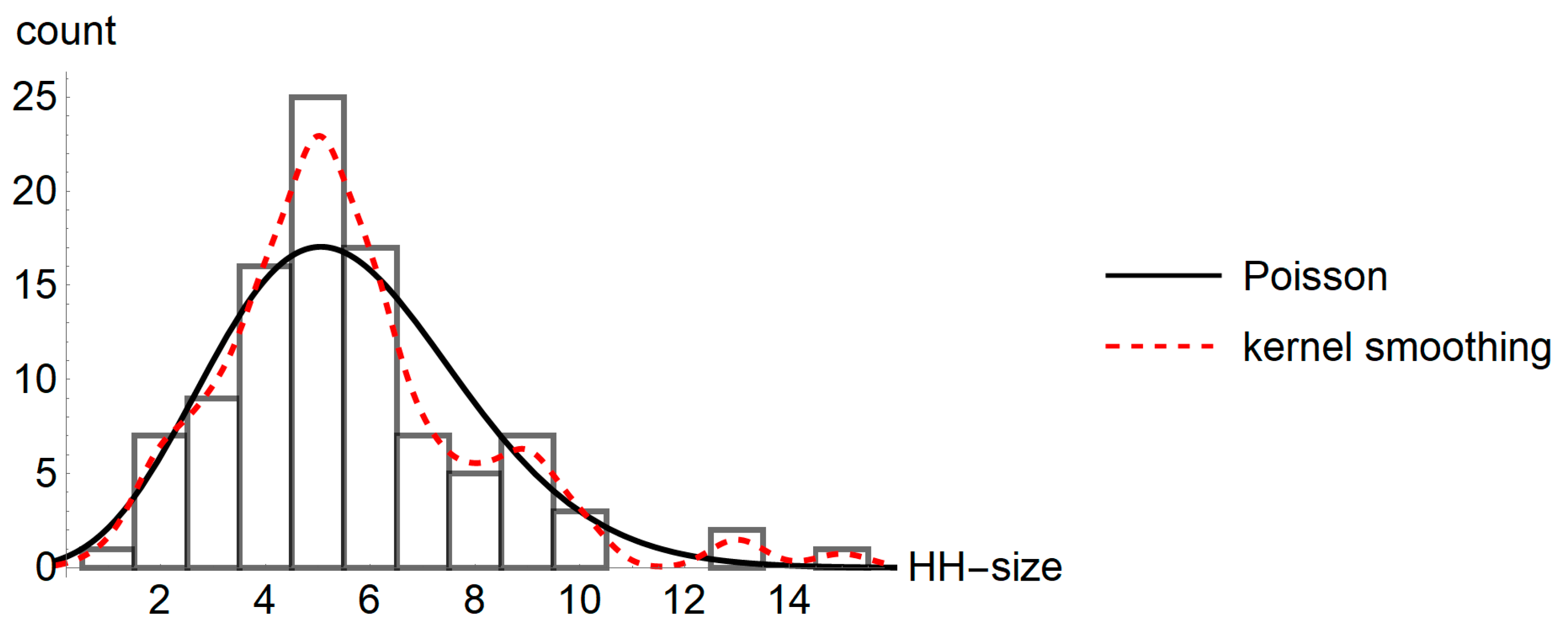
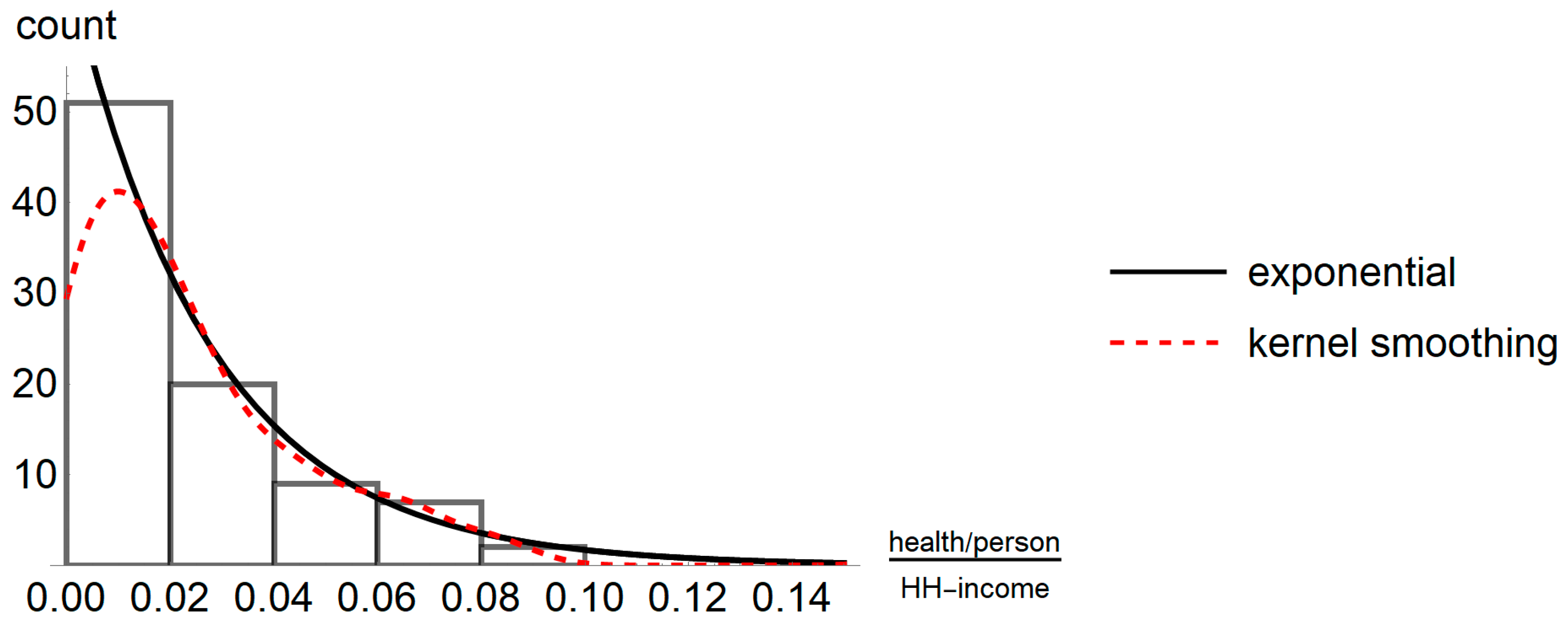
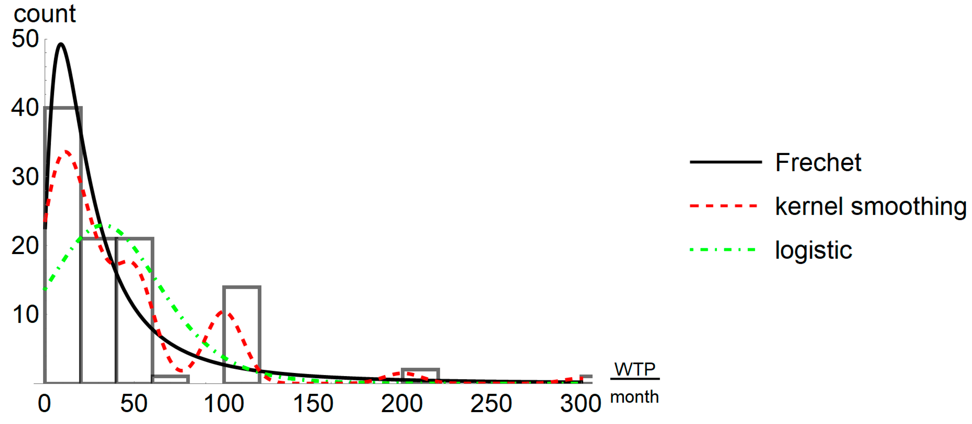
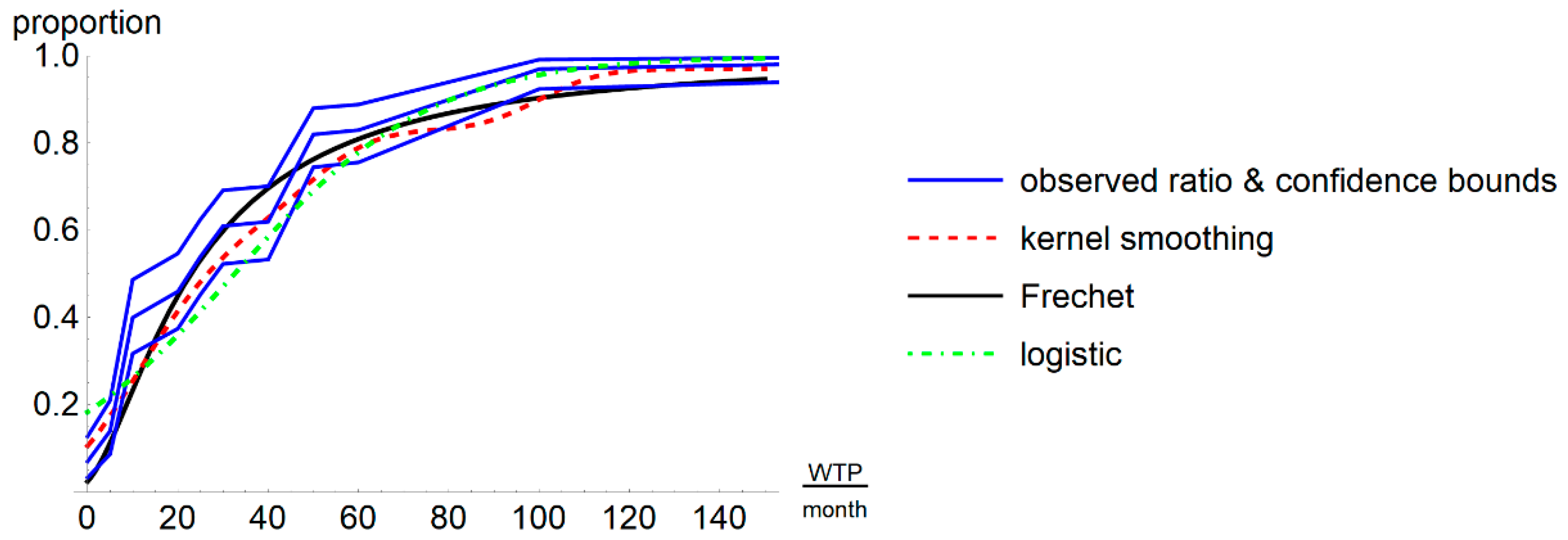
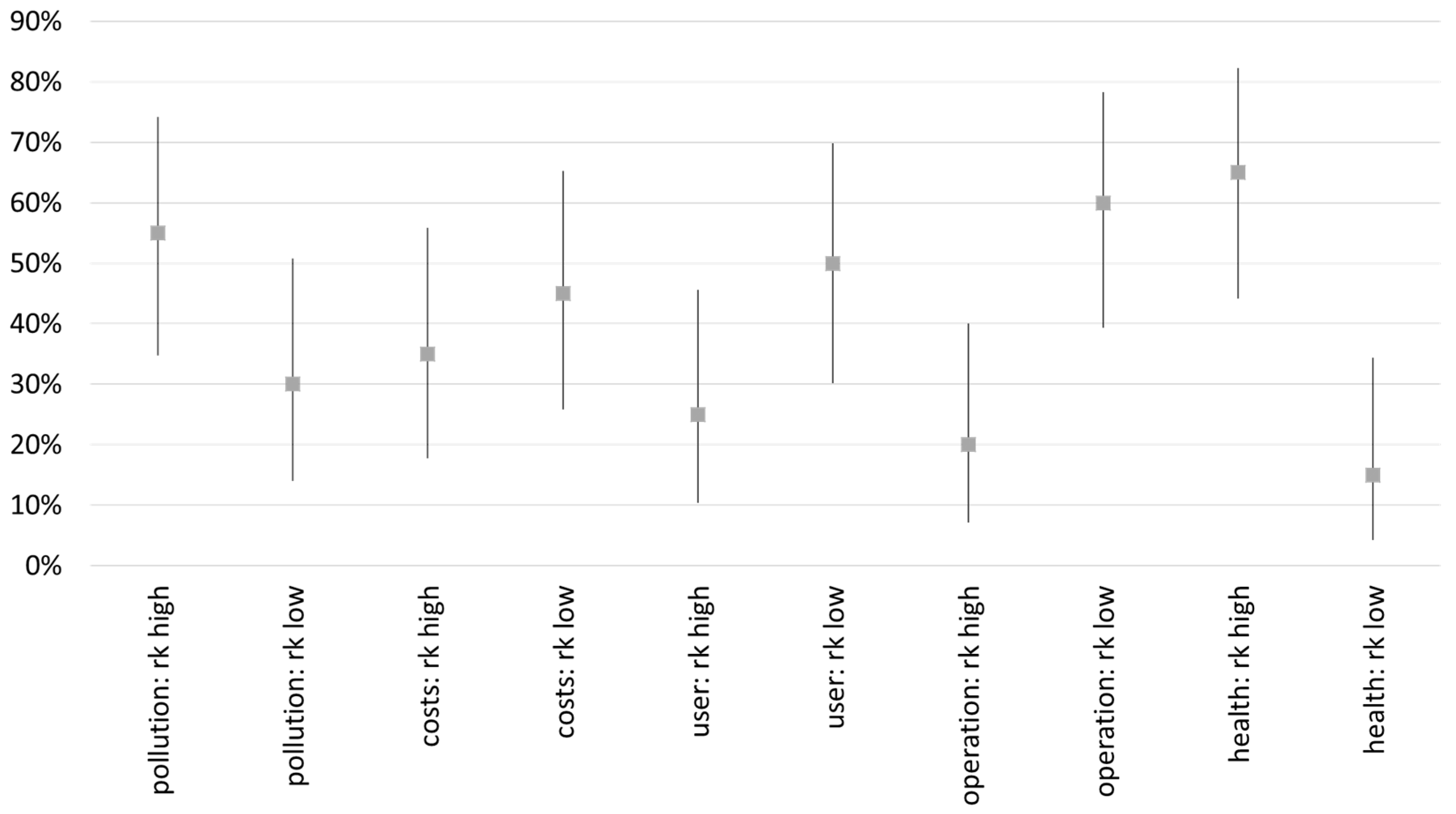
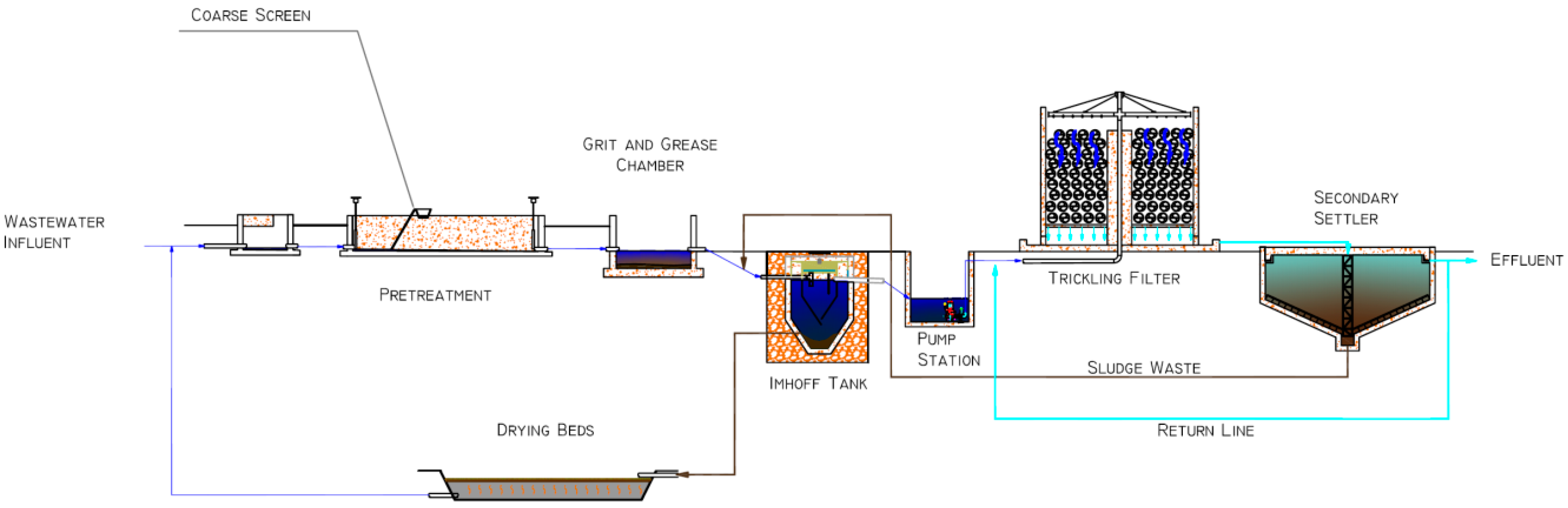
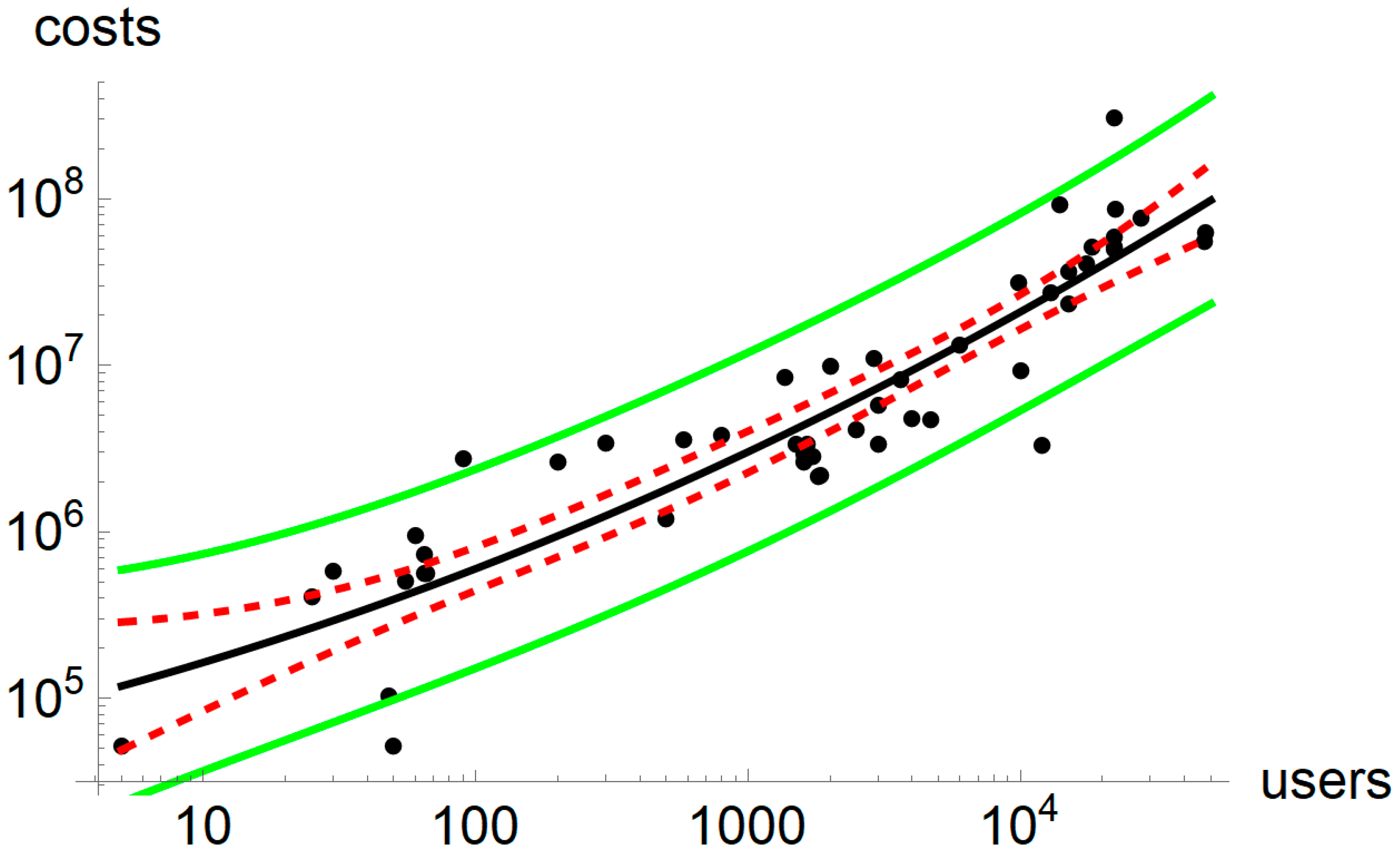
Table 1.
Criteria weights of users with consistent responses.
| ID 1 | Pollution | Costs | Comfort | O&M | Health | Class |
|---|---|---|---|---|---|---|
| Criteria Weights in Percent | ||||||
| R03 | 17 | 7 | 17 | 17 | 42 | 1 |
| R07 | 37 | 5 | 16 | 10 | 31 | 2 |
| R26 | 13 | 7 | 13 | 26 | 41 | 1 |
| R28 | 51 | 5 | 14 | 7 | 22 | 2 |
| R37 | 59 | 4 | 7 | 11 | 20 | 2 |
| R39 | 59 | 5 | 11 | 5 | 20 | 2 |
| R41 | 45 | 5 | 16 | 10 | 25 | 2 |
| R43 | 59 | 4 | 7 | 11 | 20 | 2 |
| R44 | 13 | 7 | 13 | 26 | 41 | 1 |
| R45 | 44 | 5 | 15 | 8 | 29 | 2 |
| L01 | 45 | 5 | 16 | 10 | 25 | 2 |
| L03 | 42 | 3 | 5 | 8 | 42 | 3 |
| L09 | 51 | 6 | 9 | 7 | 27 | 2 |
| L10 | 45 | 5 | 11 | 10 | 29 | 2 |
| L24 | 42 | 3 | 5 | 8 | 42 | 3 |
| L33 | 33 | 3 | 6 | 6 | 52 | 3 |
| L36 | 42 | 3 | 6 | 6 | 42 | 3 |
| L40 | 42 | 3 | 6 | 6 | 42 | 3 |
| L41 | 33 | 3 | 6 | 6 | 52 | 3 |
| L45 | 42 | 3 | 6 | 6 | 42 | 3 |
| L50 | 49 | 10 | 5 | 4 | 31 | 2 |
| I14 | 42 | 3 | 6 | 6 | 42 | 3 |
| I15 | 42 | 3 | 6 | 6 | 42 | 3 |
| I16 | 33 | 3 | 6 | 6 | 52 | 3 |
| I22 | 32 | 7 | 11 | 18 | 32 | 3 |
| I29 | 33 | 3 | 17 | 7 | 41 | 3 |
| I36 | 42 | 5 | 4 | 7 | 42 | 3 |
| I41 | 37 | 3 | 8 | 6 | 46 | 3 |
1: The ID refers to R = Mishra Talaab, L = Lalbagh and I = Indira colony.
© 2018 by the authors. Licensee MDPI, Basel, Switzerland. This article is an open access article distributed under the terms and conditions of the Creative Commons Attribution (CC BY) license (http://creativecommons.org/licenses/by/4.0/).
Share and Cite
MDPI and ACS Style
Brunner, N.; Starkl, M.; Kazmi, A.A.; Real, A.; Jain, N.; Mishra, V. Affordability of Decentralized Wastewater Systems: A Case Study in Integrated Planning from INDIA. Water 2018, 10, 1644. https://doi.org/10.3390/w10111644
AMA Style
Brunner N, Starkl M, Kazmi AA, Real A, Jain N, Mishra V. Affordability of Decentralized Wastewater Systems: A Case Study in Integrated Planning from INDIA. Water. 2018; 10(11):1644. https://doi.org/10.3390/w10111644
Chicago/Turabian StyleBrunner, Norbert, Markus Starkl, Absar A. Kazmi, Alvaro Real, Nitin Jain, and Vijay Mishra. 2018. "Affordability of Decentralized Wastewater Systems: A Case Study in Integrated Planning from INDIA" Water 10, no. 11: 1644. https://doi.org/10.3390/w10111644
Note that from the first issue of 2016, this journal uses article numbers instead of page numbers. See further details here.