Integration of a Parsimonious Hydrological Model with Recurrent Neural Networks for Improved Streamflow Forecasting

Abstract

This study applied a GR4J model in the Xiangjiang and Qujiang River basins for rainfall-runoff simulation. Four recurrent neural networks (RNNs)—the Elman recurrent neural network (ERNN), echo state network (ESN), nonlinear autoregressive exogenous inputs neural network (NARX), and long short-term memory (LSTM) network—were applied in predicting discharges. The performances of models were compared and assessed, and the best two RNNs were selected and integrated with the lumped hydrological model GR4J to forecast the discharges; meanwhile, uncertainties of the simulated discharges were estimated. The generalized likelihood uncertainty estimation method was applied to quantify the uncertainties. The results show that the LSTM and NARX better captured the time-series dynamics than the other RNNs. The hybrid models improved the prediction of high, median, and low flows, particularly in reducing the bias of underestimation of high flows in the Xiangjiang River basin. The hybrid models reduced the uncertainty intervals by more than 50% for median and low flows, and increased the cover ratios for observations. The integration of a hydrological model with a recurrent neural network considering long-term dependencies is recommended in discharge forecasting.

1. Introduction

Hydrological models are used to predict streamflows, ground water content, evapotranspiration, and other hydrological variables. Hydrological models can present rainfall-runoff processes and broaden our understanding of rainfall-runoff. However, errors and uncertainties in hydrological modeling are inevitable due to limited knowledge of the hydrological system, forcing and response data, and simplification of the real world [1,2].

Prediction errors are often presented as underestimation or overestimation in the discharge predicted by a hydrological model. Errors can measure the performance of a model and serve as bases to improve the prediction accuracy against observation by regression analysis. Errors contain information about both observations and models; thus, they can be used to improve forecasting [3,4,5]. Uncertainty is often quantified as a range of prediction error. It is propagated through observation, parameterization, and model structure [6]. Alleviating the errors and controlling the range of uncertainties is one of the main issues of hydrological forecasting. In predicting, since extreme flows are in the tails of the hydrologic frequency distribution and less information is available, uncertainties in extreme flows are often larger than those in the mean flows, which make it more difficult to forecast [7,8].

There are various approaches to handle errors. Many studies quantified uncertainty in hydrological modeling by using Bayesian methods [9,10,11] or the generalized likelihood uncertainty estimation (GLUE) approach [12,13,14]. Besides, attempts have been made to improve forecasting accuracy through reducing uncertainty by developing more sophisticated physically-based hydrological models [15], using more accurate input data [16,17,18], and applying error-correction methods such as Kalman filtering, fuzzy logic, and autoregressive (AR) processes [4,5,19]. AR models are a commonly used error correction method because of their simplicity; they are more efficient than artificial neural networks (ANNs) and other nonlinear autoregressive methods [4]. However, AR models are linear, which is a disadvantage in representing the nonlinear dynamics inherent in hydrological processes [20].

When complete and accurate forcing data is unavailable to hydrological modelers, it makes data-driven methods appealing for hydrological prediction. A number of methods have been widely used in streamflow, drought, and groundwater level prediction, such as support vector machine (SVM) and ANNs with various structures, including multilayer perceptrons (MLPs), neuro-fuzzy neural networks (NFNNs), back propagation artificial neural networks (BPNNs), and recurrent neural networks (RNNs) [21,22,23,24,25,26]. A feed-forward artificial neural network such as a BPNN does not treat temporal ordering as an explicit feature of time series, so it has difficulty in dealing with the short-term dynamics of a nonlinear system [27]. RNNs contain blocks that can remember information for an arbitrary length of time. They can retain information from previous samples, and are thus suitable for capturing the dynamic behavior of time series by recurrently sending information in current layers forward to other layers [28].

In this study, a parsimonious hydrological model that is a lumped one with only four parameters and four types of RNNs are integrated to improve the streamflow forecasting. RNNs have been used for prediction in several recent studies [29,30,31,32]. For example, Change et al. used back propagation neural network (BPNN), Elman recurrent neural network (ERNN), and nonlinear autoregressive networks with exogenous inputs (NARX) to forecast inundation levels during flood periods [32]. Chen et al. applied a reinforced neural network (R-RTRL NN) to improve multi-step ahead forecasts of reservoir inflow during typhoon events [31]. Liang et al. made forecasts of the Dongting Lake water level based on a long short-term memory network [33]. RNNs have been used independently in the studies mentioned above, and the results have been compared with static models rather than with other RNNs. There is little comprehensive analysis of the RNN’s performance in predicting streamflow, and the uncertainties of hydrological modeling are also an important issue that few studies have covered. Since prediction errors carry information about both observations and model performance, improvement can be expected in streamflow prediction by integrating an RNN with a hydrological model.

Four different kinds of RNNs (ERNN, ESN, NARX, and LSTM) are applied to assess their ability in forecasting the discharges and study their influences on modeling uncertainties by integrating with a hydrological model. Therefore, the main objectives of the study are: (1) to compare the performance of the RNNs and the hydrological model in streamflow prediction; (2) to assess the improvement in the forecasting of streamflow gained by integrating a hydrological model and networks in the data-driven approach; and (3) to quantify the effect of incorporating error correction on forecasting uncertainty.

2. Materials and Methods

2.1. Data and Study Area

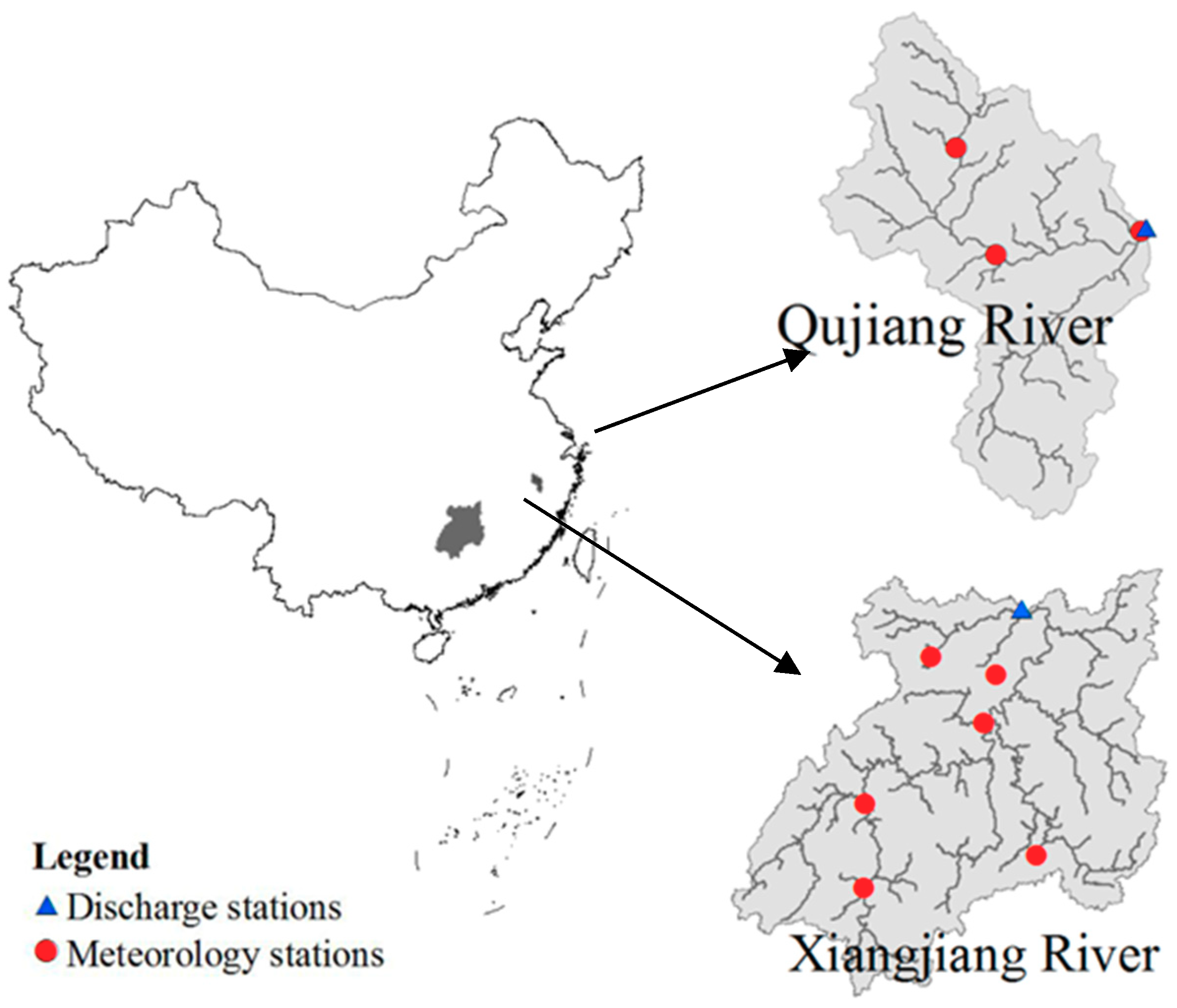
Two geographically separated river basins of different sizes were selected as study areas for comparison: the Xiangjiang River, a tributary of the Yangtze River in central southern China with a drainage area of ~81,600 km²; and the Qujiang River located in eastern China with a drainage area of 5290 km². Figure 1 shows the location and tributaries of the rivers together with the observation stations. Overlapping time series data for 15 years (1981–1995) of observed daily precipitation, temperature, and discharges from each station were used. Ten years of the data (1981–1990) were used for model calibration, and the other five years (1991–1995) were used for model validation. Both the Xiangjiang River basin and the Qujiang River basin have a mean annual total precipitation of ~1500 mm, and are dominated by the subtropical high climate system, which features a hot and rainy summer. The Xiangjiang River is sourced from Yongzhou, and flows northward to the Yangtze River, with a total length of 844 km. The major land-use types of the Xiangjiang River basin are forests, paddy field, rainfed cropland, and meadow. The Qujiang River is sourced from Huangshan, and flow northeast to the Qiantang River, with a total length of 522 km. The major land-use type of the Qujiang River basin is farmland, which accounts for 88%. Due to differences in the topography and the size of the drainage area, the maximum daily discharge of the Xiangjiang basin (20,600 m³/s) is about four times greater than that of the Qujiang basin discharge (4800 m³/s).

2.2. GR4J Model

The GR4J daily catchment water balance model, which has only four parameters, is used in this study, and it has been effectively and extensively used worldwide for many areas [34,35]. The GR4J models input include precipitation and potential evapotranspiration (PET). The four parameters are: X1 (mm), the capacity of the production reservoir; X2 (mm), the catchment groundwater exchange coefficient; X3 (mm), the maximum daily capacity of the routing reservoir; and X4 (days), the time base of the unit hydrograph. The model has four subroutines: the soil moisture subroutine, the effective precipitation calculation subroutine, the slow flow subroutine, and the quick flow subroutine. GR4J obtains net rainfall by subtracting potential evapotranspiration from precipitation. Net rainfall is divided into two parts: one part goes into the production reservoir where evaporation and percolation occur, and the other part goes directly to the flow routing reservoir. Water in the production reservoir reaches the flow routing reservoir through infiltration. The two flow components are combined and then split into 90% runoff routed by a unit hydrograph to the nonlinear routing reservoir and 10% runoff routed by a single unit hydrograph to runoff. The total runoff is obtained by adding these two runoffs together.

In terms of the sole model simulation, the performances of the hydrological model are compared with the RNNs that are described in the following sections using the same input data. In terms of the integration, the error in the output from GR4J is given by subtracting observation from prediction. The error, together with precipitation and PET, is then used as input to the RNNs to forecast the error in the next time step. The opposite value of estimated error from the RNN is added back to the discharge obtained by GR4J as the final predicted discharge.

$$Er{r}_G\left(t\right)=Q_{SG}\left(t\right)-Q_o\left(t\right)$$

(1)

$$Er{r}_p\left(t+1\right)=f\left(Er{r}_G\left(t\right),P\left(t+1\right),PET\left(t+1\right)\right)$$

(2)

$$Q_{SI}\left(t+1\right)=Q_{SG}\left(t+1\right)-Er{r}_p\left(t+1\right)$$

(3)

where $Er{r}_G$ and $Er{r}_p$ represent the error from the GR4J modeling, and the predicted error with RNNs. $Q_o$, $Q_{SG}$, and $Q_{SI}$ represent the observed discharges, simulated discharges with GR4J, and forecasted discharges with the integration model, respectively. P and PET represent the precipitation and potential evapotranspiration. $t$is the time step. $f()$ represents the integrated RNN.

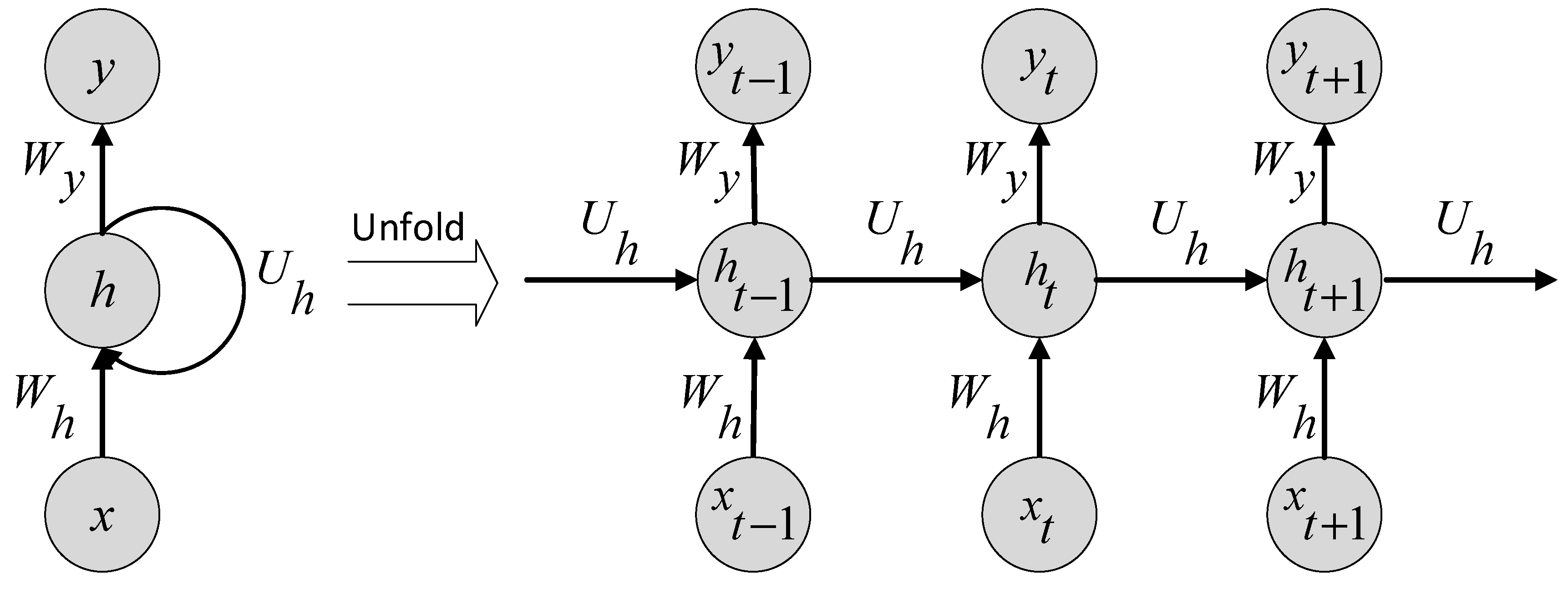
2.3. Elman Recurrent Neural Network

The Elman recurrent neural network (ERNN) is a three-layer recurrent neural network [36]. It is the basis for more complex RNN architectures. The ERNN architecture is shown in Figure A1 in the Appendix A. There are input layers, hidden layers, and output layers in the ERNN. At each time step, the input is fed forward, and a learning rule is applied to update the parameters, which takes past states into account through recurrent connections. The output from the hidden layer h(t − 1) at time t − 1 is kept (as a past state), together with the input x(t) for time t, are then fed back to the hidden layer at time t. In this way, the context units always maintain a copy of the previous values in the hidden layers. The equations for the state and output of the ERNN are:

$$h\left(t\right)=f\left(W_{h}x\left(t\right)+U_{h}h\left(t-1\right)+b_h\right)$$

(4)

$$y\left(t\right)=g\left(W_{y}h\left(t\right)+b_y\right)$$

(5)

where f(∙) is the activation function (a sigmoid function) of the hidden layers; g(∙) is the transformation function (a softmax function) for the output layer; h(t) is a hidden layer that represents the content of the network at time step t; $W_h$, $U_h$, and $W_y$ are the weighted variance matrices between the input and the hidden layers, the context units and the hidden layers, and the hidden layers and the output, respectively; $b_h$ and $b_y$ are bias vectors for the hidden layers and the output layers, respectively; and $x\left(t\right)$ and $y\left(t\right)$ are the input and output at time step t. ERNN in this study is developed in Matlab. Parameters are optimized using gradient descent with momentum and adaptive learning rate back propagation [37]. There are 30 hidden units in the recurrent hidden layer. The mean squared error is used as the loss function. The network is trained for 1000 epochs for calibration.

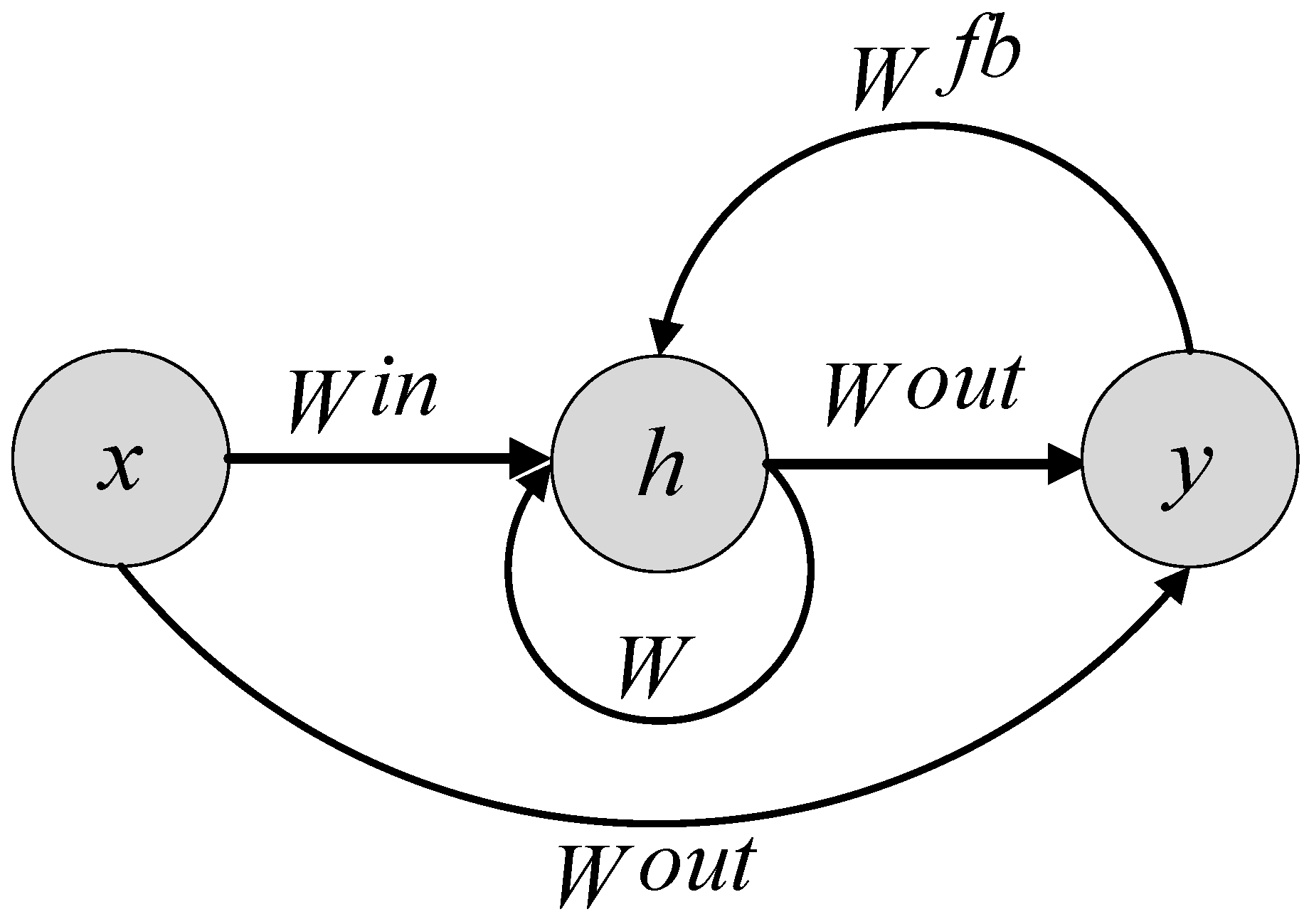
2.4. Echo State Network

Training and optimizing the parameters in an RNN is computationally expensive, and can sometimes lead to local minima in high-dimensional problems. The echo state network (ESN) provides an alternative to train and use RNNs. An echo state network is a three-layer recurrent neural network with a sparsely and randomly connected hidden layer [38,39], as shown in Figure A2 in the Appendix A. The ESN is composed of an input layer, a hidden layer (known as the reservoir) consisting of large, random, and fixed neural networks that receive input signals, and an output layer that produces output by a linear or nonlinear combination of the reservoir signals. The outputs are sent back to the reservoir. The equations for the state and the output of the ESN are:

$$h\left(t\right)=f\left(W^{in}x\left(t\right)+Wh\left(t-1\right)+W^{fb}y\left(t-1\right)+ϵ\left(t-1\right)\right)$$

(6)

$$y\left(t\right)=g\left(W^{out}\left[x\left(t\right);h\left(t\right)\right]\right)$$

(7)

where x(t) and y(t) are respectively the input and output at time step t; $h\left(t\right)$ is the hidden layer at time step$t$; $W^{in}$ is the weight between the input and the hidden layer; $W$ is the weight between the previous state and the current state of the hidden layer; $W^{fb}$ is the weight between the previous output and the hidden layer; and $W^{out}$ is the weight between the concatenation of the input and hidden layer and the output; [;] represents vector concatenation; $ϵ\left(t-1\right)$ is noise; and $f(·)$ is the sigmoid function.

A variant of the basic ESN is an ESN with leaky integrator neurons. This kind of neurons not only controls the input and output feedback scaling and the spectral radius of the reservoir, but also controls the leaking rate. Such an ESN is more suitable for modeling a dynamic system. The equation for the state can be expressed as:

$$h\left(t\right)=\left(1-\alpha \gamma \right)h\left(t-1\right)+\gamma f\left(W^{in}x\left(t\right)+Wh\left(t-1\right)+W^{fb}y\left(t-1\right)+ϵ\left(t-1\right)\right)$$

(8)

where α > 0, γ > 0, αγ < 1, α and γ are parameters for the leaky integrator neurons, and α > 0 is the leaky decay rate. An ESN with leaky integrator neurons is used in this study. It contains 30 reservoir units; the spectral radius is set to 0.5; input and output feedback scaling are in the interval [0.1, 1]; all of the weights are fixed with randomly chosen values in the interval [–1, 1] having a uniform distribution. $W^{out}$ is going to be trained, and the training process is called teacher forcing, which is accomplished by solving a convex problem using stochastic gradient descent.

2.5. Nonlinear Autoregressive Exogenous Inputs Neural Network

A nonlinear autoregressive exogenous inputs neural network (NARX) is a recurrent neural network with several hidden layers that is suitable for modeling nonlinear systems, especially a time series [40]. Gradient-descent learning can be more effective in NARXs than in other recurrent architectures, and gives better performance for a time series with long-term dependencies [41,42]. The predicted value at the tth time step, y(t), can be expressed as:

$$y\left(t\right)=\varphi \left(y\left(t-1\right),\dots ,y\left(t-d_y+1\right),x\left(t\right),x\left(t-1\right),\dots ,x\left(t-d_x\right)\right)$$

(9)

where $\varphi (·)$ is the nonlinear mapping function performed by a multilayer perceptron (MLP); x(t) is the input at time $t$; and $d_x$ and $d_y$ are the input and output lags, with $d_y\ge 1$, $d_x\ge 1$, and $d_y\ge d_x$.

NARX architecture is shown in Figure A3 in the Appendix A. The NARX model in this study is developed using Matlab. In training the NARX parameters, the output from the network is fed back with the input, and the parameters can be obtained by a quasi-Newton search, the Levenberg–Marquardt algorithm [43]. The loss function is the mean squared error. There are 10 hidden layers, and the network is trained for 1000 epochs.

2.6. Long Short-Term Memory

RNNs often experience the problem that error signals can either explode or vanish after several steps of propagating to previous layers. NARXs provide an orthogonal mechanism to deal with such problems by using a single factor, which represents the number of delays [44]. The long short-term memory (LSTM) network also deals with the vanishing gradient or exploding problems. A long short-term memory (LSTM) network is a special type of recurrent neural network. It was first developed by Hochreiter and Schmidhuber [45] and then refined by many other researchers [46,47,48]. It preserves states over long periods of time without a loss of short-term dependencies by introducing gates to blocks [45]. The gates help the LSTM network decide what to forget and what to remember, so it avoids error signal decay by keeping the errors in memory. This feature of LSTM is also suitable for discharge forecasting, where the predicted discharge is related to previous simulations over a long period. LSTM networks have gained attention recently because of their capacity to remember information for a long time. LSTMs are effective in making time-series predictions for air pollution [49], sewer overflow monitoring [50], rainfall-runoff modeling [51], and lake water level forecast [33].

Similar to other RNNs, the LSTM network consists of an input layer, an output layer, and a number of hidden layers, and the architecture has the form of a chain of repeating modules of neural networks. The repeating module, called a cell, has five different components that are altered by three gates (input, output, and forget gates). The behavior of the gates is controlled by a set of parameters that can be trained by the descending gradient descent method. The LSTM architecture is shown in Figure A4 in the Appendix A. The equations for the forward pass of an LSTM cell are:

$$\mathrm{forget}\mathrm{gate}:{\sigma }_f\left(t\right)=\sigma \left({\mathrm{W}}_{\mathrm{f}}x\left(t\right)+{\mathrm{R}}_{\mathrm{f}}y\left(t-1\right)+b_f\right)$$

(10)

$$\mathrm{input}\mathrm{gate}:{\sigma }_i\left(t\right)=\sigma \left({\mathrm{W}}_{\mathrm{i}}x\left(t\right)+{\mathrm{R}}_{\mathrm{i}}y\left(t-1\right)+b_i\right)$$

(11)

$$\mathrm{output}\mathrm{gate}:{\sigma }_o\left(t\right)=\sigma \left({\mathrm{W}}_{\mathrm{o}}x\left(t\right)+{\mathrm{R}}_{\mathrm{o}}y\left(t-1\right)+b_0\right)$$

(12)

$$\mathrm{cell}\mathrm{state}:h\left(t\right)={\sigma }_f\left(t\right)\odot h\left(t-1\right)+{\sigma }_i\left(t\right)\odot g_1\left({\mathrm{W}}_{\mathrm{h}}x\left(t\right)+{\mathrm{R}}_{\mathrm{h}}y\left(t-1\right)+b_h\right)$$

(13)

$$\mathrm{output}:y\left(t\right)={\sigma }_o\left(t\right)\odot g_2\left(h\left(t\right)\right)$$

(14)

where $x\left(t\right)$ and $y\left(t\right)$ are the input and output at time $t$;$h\left(t\right)$ is the cell state at time $t$; ${\mathrm{W}}_{\mathrm{f}}$, ${\mathrm{W}}_{\mathrm{i}}$, ${\mathrm{W}}_{\mathrm{o}}$, and ${\mathrm{W}}_{\mathrm{h}}$ are the weights for the input; ${\mathrm{R}}_{\mathrm{f}}$, ${\mathrm{R}}_{\mathrm{i}}$, ${\mathrm{R}}_{\mathrm{o}}$, and ${\mathrm{R}}_{\mathrm{h}}$ are the weights for the recurrent output; $b_f$, $b_i$, $b_o$, and $b_h$ are biases; $\sigma (·)$ is a sigmoid function; and $g_1(·)$ and $g_2(·)$ are pointwise nonlinear activation functions. The operator $\odot$ denotes the Hadamard product (entrywise multiplication). The forget gate ${\sigma }_f$ determines what information to discard from the previous cell state. The input gate controls how much to update the new cell state with candidate values. The output gate, a sigmoid function, decides the parts of the cell states to output. All three gate functions are relative to the input and the output of the previous time step. The LSTM in this study is developed using the deep learning framework Keras. There are 50 hidden neurons in the hidden layer. The initial weights of the LSTM are sampled from a uniform distribution in the interval [0, 1] and rescaled by 2%. The loss function is the mean squared error, and adaptive moment estimation (Adam) is used as the optimization algorithm.

2.7. Measurement of Performance

Three statistical indicators—the Nash–Sutcliffe efficiency coefficient (NSE), the root mean square error (RMSE), and mean absolute percentage error (MAPE)—are used in this study to evaluate the performance of the hydrological models and RNNs. The equations of the indicators are:

$$\mathrm{NSE}=1-\frac{{{\displaystyle \sum }}_{t=1}^T{\left(Q_o^t-Q_s^t\right)}^2}{{{\displaystyle \sum }}_{t=1}^{\mathrm{T}}{\left(Q_o^t-{\overline{Q}}_o\right)}^2}$$

(15)

$$\mathrm{RMSE}=\sqrt{\frac{1}{T}{\displaystyle \sum }_{t=1}^T{\left(Q_o^t-Q_s^t\right)}^2}$$

(16)

$$\mathrm{MAPE}=\frac{1}{T}{\displaystyle \sum }_{t=1}^T\frac{\left|Q_o^t-Q_s^t\right|}{Q_o^t}$$

(17)

where $Q_o^t$ is the observed discharge at time t; $Q_s^t$ is the simulated discharge at time t; and T is the length of the time series. The discharges were categorized into high, medium, and low flows to compare the accuracy of the hybrid models for different discharge levels in the basins. High flow is the discharge above the 90th percentile of the 15-year daily discharges; low flow is the discharge below the 10th percentile of the 15-year daily discharges; and medium flow is in between.

2.8. Quantification of Uncertainty

The generalized likelihood uncertainty estimation (GLUE) method was used to estimate the range of uncertainty for the predicted discharges from various model parameters. GLUE is based on the concept of equifinality, which indicates there are many parameter sets and models that can lead to good representations of the rainfall-runoff process [52]. The major steps of GLUE include:

(1)

10,000 parameter sets are generated from the uniform distribution with upper and lower boundaries for each parameter. Previous studies involving an application of the GR4J model are used as references for the boundaries. The ranges of the parameters (

Table 1. Ranges of parameters of the GR4J model.

Parameters	Description	Minimum	Maximum	Unit
X1	Capacity of the production reservoir	10	2000	mm
X2	Groundwater exchange coefficient	−8	6	mm
X3	One day capacity of the routing reservoir	10	500	mm
X4	Time base of the unit hydrograph	0	4	d

) cover most reasonable values [34,53,54].

(2)

Definition of the likelihood function and choosing the threshold value for the behavioral parameter sets. NSE is used as the likelihood function. The threshold is defined as 0.7 [54], which means that parameter sets with an efficiency <0.7 are rejected.

(3)

Calculation of the posterior likelihood distribution based on the prior distribution and likelihood.

(4)

Estimation of the uncertainty range. Outcomes that fall between the fifth and 95th percentiles are used to calculate the uncertainty ranges.

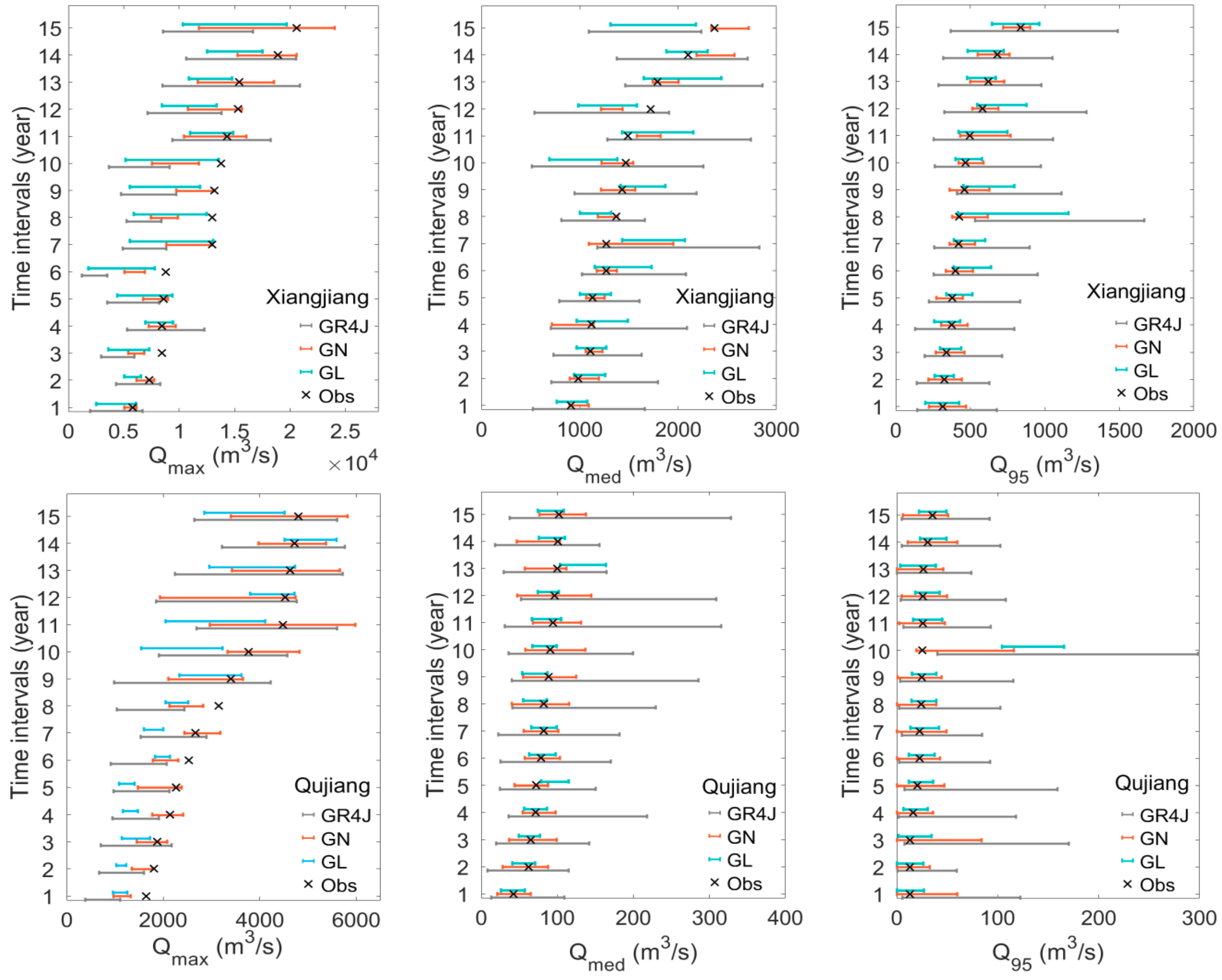
The uncertainties of high, median, and low flows were assessed individually. The annual maximum daily discharge (Qmax), the annual median daily discharge (Qmed), and the annual daily discharge of the fifth percentile (Q95) were used to represent extremely high flow, median flow, and extremely low flow, respectively.

3. Results

3.1. Model Evaluation and Error Diagnostics

The calibration and validation results for the discharge of the two river basins given by GR4J and the RNNs are compared in

Table 2. Performance indicators of the hydrological model GR4J and different recurrent neural networks (RNNs). MAPE: mean absolute percentage error, NSE: Nash–Sutcliffe efficiency coefficient, RMSE: root mean square error.

Gauge Stations	Models	Calibration			Validation
		NSE	RMSE (m3/s)	MAPE	NSE	RMSE (m3/s)	MAPE
Xiangjiang	GR4J	0.860	724	0.223	0.869	837	0.189
	ERNN	0.381	1522	0.672	0.450	1725	0.470
	ESN	0.745	970	0.428	0.780	1088	0.360
	NARX	0.936	489	0.103	0.934	595	0.096
	LSTM	0.933	500	0.091	0.932	608	0.086
Qujiang	GR4J	0.933	90	0.281	0.936	122	0.336
	ERNN	0.664	201	1.349	0.713	259	1.320
	ESN	0.889	116	0.683	0.906	148	0.663
	NARX	0.933	89	0.243	0.938	120	0.241
	LSTM	0.929	92	0.336	0.946	112	0.348

Note: Bold text represents the best performance in the column.

. Comparison among RNNs shows good agreement between observed discharges and the predicted discharges of the NARX, ESN, and LSTM. The statistical indices for both basins show that the NARX and LSTM, which both have long-term memory in their architecture, provide the most accurate estimates, followed by ESN. ERNN performs the worst. Note that all of the RNNs and hydrological models that were used in the study are more accurate for the Qujiang basin, which has a smaller catchment area, smaller peak flows, and less variance in the hydro-meteorological time series, than those for the Xiangjiang basin. Besides, the Qujiang River basin has a higher meteorology station density than the Xiangjiang River basin, which could provide more wholesome information for the models. The NARX and LSTM are more accurate than GR4J for the Xiangjiang basin. However, GR4J performs well for the Qujiang basin, having similar index values with the NARX and LSTM; NSE for GR4J increases to >0.93.

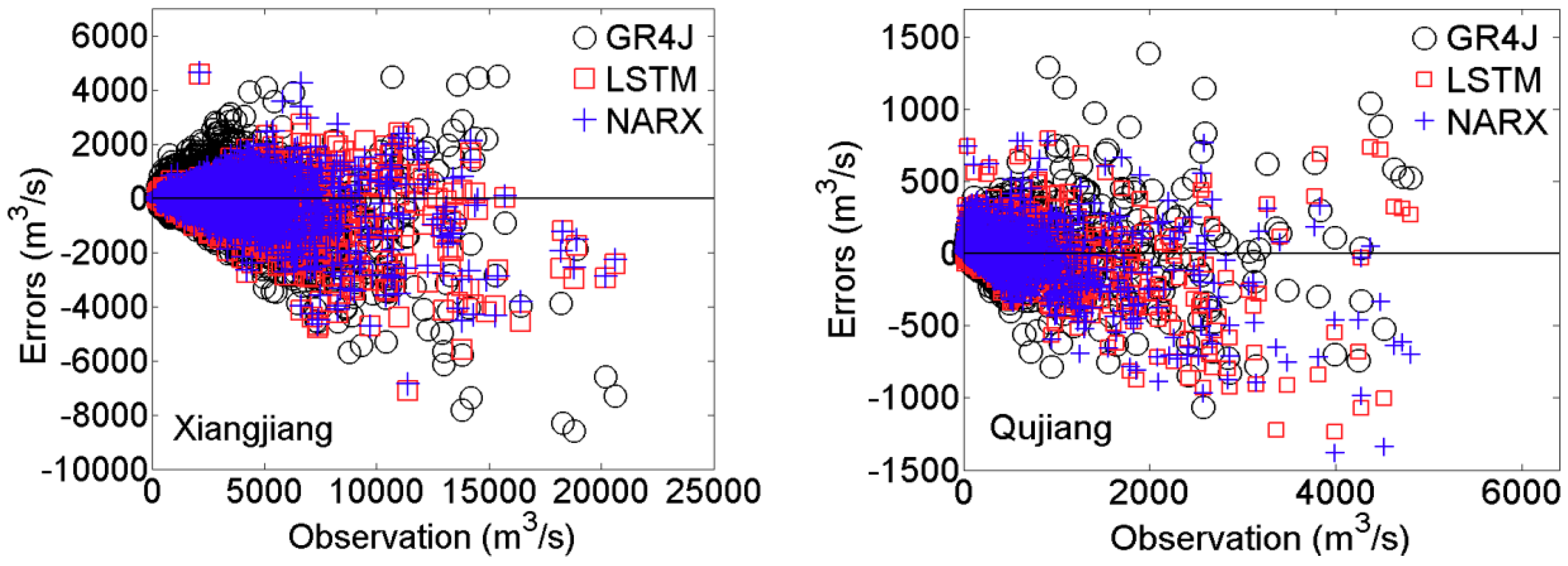
Figure 2 shows the errors (prediction minus observation) of discharge predictions for the Xiangjiang and Qujiang basins with the GR4J, NARX, and LSTM models. In general, the errors increase with the volume discharged. All three models tend to underestimate the higher volumes in the Xiangjiang basin, and GR4J more so than the NARX and LSTM. Note that for the Qujiang basin, the largest overestimate given by GR4J is at ~2000 m³/s rather than at higher volumes, and there are both underestimates and overestimates by all three models.

3.2. Integration of GR4J with RNNs

Analysis of the performance indicators shows that the LSTM and NARX are the best RNNs to forecast discharges. They show a good match between forecasting and observation for both basins. The hydrological model GR4J was integrated with LSTM (referred to as GL) and NARX (referred to as GN) to improve forecasting. The major difference between the GR4J model and the hybrid model is that the hybrid model combines the data-driven models with the GR4J model. The GR4J model used precipitation and PET as input, while the GL and GN models used errors from the GR4J model simulation, which contains the information from discharges at previous time steps. It makes the hybrid model more advantageous in fully utilizing the available data.

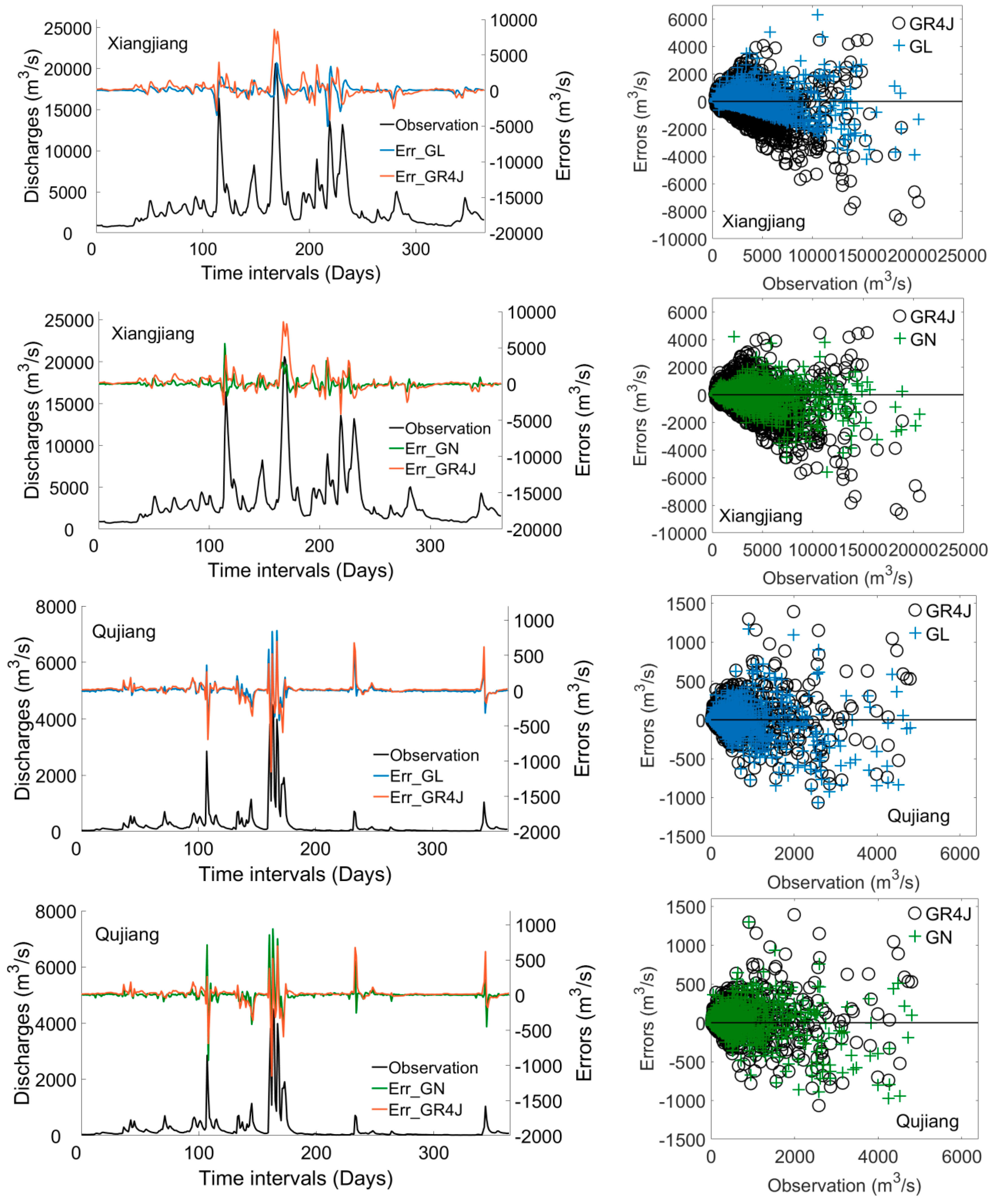
The statistical indicators for the hybrid models are given in

Table 3. Performance indicators for GR4J and the hybrid models.

Gauge Stations	Models	Calibration			Validation
		NSE	RMSE	MAPE	NSE	RMSE	MAPE
Xiangjiang	GR4J	0.860	724	0.223	0.869	837	0.189
	GL	0.954	414	0.098	0.952	510	0.098
	GN	0.954	414	0.098	0.957	480	0.085
Qujiang	GR4J	0.933	90	0.281	0.936	122	0.336
	GL	0.942	83	0.210	0.954	104	0.221
	GN	0.942	83	0.210	0.955	102	0.181

. The results show that the hybrid models are more accurate than GR4J, especially in the Xiangjiang basin. It could be explained that the hybrid model has more input data, which involves the error information in the previous time steps, and the RNNs learns the information and makes a correction on the next time step. The improvement of the discharges by hybrid models are less in the Qujiang River basin. Figure 3 shows the performance and the prediction errors of the GR4J model and the hybrid models (right side) in 1994, when there were several floods in both basins. The figure shows that in both basins, GL and GN perform similarly. Despite a few overcorrected points, the advantages of the hybrid models (both GL and GN) are more obvious when the flow is >14,000 m³/s, which is where the GR4J model severely underestimates. Errors in hybrid model forecasting for high flows tend to be less biased in the Xiangjiang basin. For the Qujiang basin, GR4J has given good forecasting for the high flows, but the hybrid models could not.

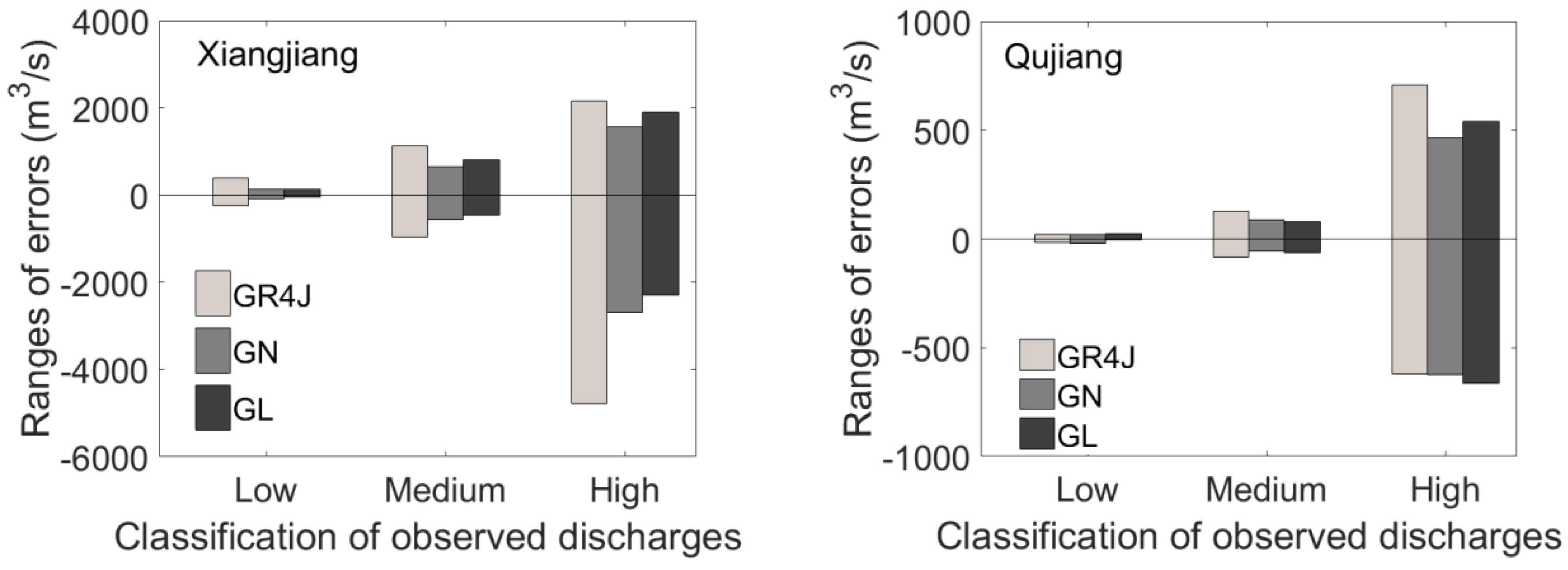
Figure 4 shows the range of errors for low, medium, and high flows with 95% confidence intervals. A positive value represents overestimation, and a negative value represents underestimation. If measured with absolute values, the greatest improvement for the Xiangjiang basin is found in the forecasting of high flow, where the underestimation by the GR4J model was reduced from >4000 m³/s to ~2000 m³/s by GN and GL. If measured with relative percentage, the low flows improved a lot, with errors reduced by 66% by GN and 63% by GL. The forecasting of high flow in the Qujiang basin was more accurate and improved with less magnitude: overestimation of high flow by GR4J was reduced by ~100 m³/s by GN and GL.

3.3. Uncertainty in the Integrated Models

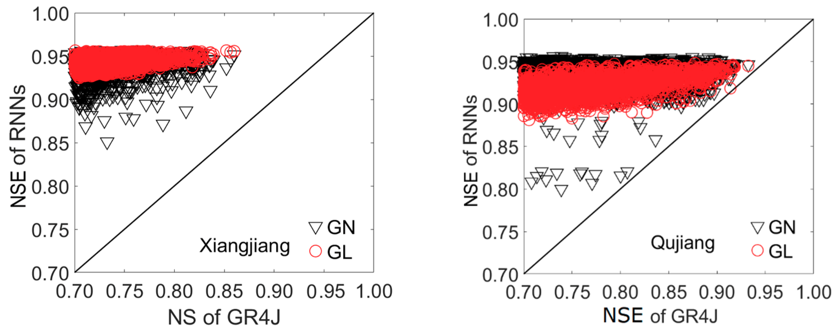
A parameter set that gives an NSE value >0.7 is regarded as behavioral, and the uncertainty range of the predicted discharge values is related to the behavioral parameter set. Hereafter, GR4J and all of the behavioral parameter sets are integrated with the NARX and LSTM. Figure 5 shows the NSE values for GR4J versus the NSE values of GN and GL for both basins. Both GN and GL values are above the solid line, and as the NSE value of GR4J increases, the line gets closer to the circles and triangles. The figure shows that GN and GL perform better than GR4J in terms of NSE, as expected. It is partly due to the additional data that was used as input in the GN and GL models. The improvement is more obvious for the models with low NSE values than for those with high NSE values. The circles converge better than the triangles, indicating that the performance of the GL model is more stable than that of the GN model.

Figure 6 shows the uncertainty ranges of Qmax, Qmed, and Q95 ranking from low to high in each of the 15 years by GR4J, GN, and GL in both river basins. The forecasting of high flows is more uncertain than that of low flows. GR4J has greater uncertainty intervals than GN and GL for extremely high, median, and extremely low flows in most cases, and there are some uncertain intervals from GR4J that did not cover the observed values, particularly in underestimates of high flows in both the Xiangjiang and Qujiang basins.

Table 4. Average uncertainty intervals and cover ratios of Qmax, Qmed, and Q95 with GR4J, GN, and GL.

River Basin	Criteria	Qmax		Qmed		Q95
		Uncertainty Interval	Cover Ratio	Uncertainty Interval	Cover Ratio	Uncertainty Interval	Cover Ratio
Xiangjiang	GR4J	5950	0.40	1250	0.93	725	0.93
	GN	3975	0.60	315	0.80	215	1.00
	GL	5200	0.33	525	0.67	265	1.00
Qujiang	GR4J	1990	0.60	175	1.00	115	0.93
	GN	1325	0.73	60	1.00	50	1.00
	GL	890	0.27	35	0.80	30	0.93

Note: Bold texts represent the best performance of the model in corresponding river basins.

shows the mean uncertainty intervals and cover ratios of Qmax, Qmed, and Q95 by the models for both basins (the cover ratio is the proportion of observations that are within the uncertainty interval). The smallest uncertainty intervals and the largest cover ratios among the three models are in boldface. In most cases, GN has the smallest uncertainty interval and the highest cover ratio, especially for extremely high and extremely low flow forecasting, in both basins. Although GR4J has a higher cover ratio for Qmed in the Xiangjiang basin than both GN and GL, the uncertainty intervals were reduced by more than 50%. The GL model had smaller uncertainty intervals than both the GN and GR4J models in the Qujiang basin, but at the expense of the cover ratio.

4. Discussion

GR4J is a lumped hydrological model, and this study showed that it is more suitable for the smaller Qujiang basin, which tends to be more spatially homogeneous than the larger basin. Thus, if a larger catchment is treated as being homogeneous, more errors will be produced. The GR4J model combines physical processes in a simplified form, whereas the RNNs are black boxes that do not model physical processes, and are without the need for predetermined equations as the processes-based models. GR4J produces results by gaining information directly from the time-series data. The hybrid model could utilize the extra information from discharges at previous time steps. The lumped model is inferior to the NARX and LSTM models acting on the same input datasets when the hydrology condition is complex and there is a limited representation of hydrological processes. The integrated models have a better performance than any single model in this study, since the error information from previous simulations are used as input in the hybrid models, which contribute to the improvement to some extent.

RNNs are neural networks that have at least one feedback loop from previous computations, which enables them to store (or remember) information when processing new input data. However, some types of RNNs did not provide accurate forecasting in this study; GR4J outperformed ERNN and ESN, although it is inferior to the LSTM and NARX. The RNNs with more complex architecture, LSTM and NARX, can better predict discharges. The architecture (Figure A1) shows that the hidden layers can retain information from previous time steps as memory for the present time step, but the vanishing gradient problem reduces the network’s ability to use information from distant time steps. If a catchment stores water such that discharge at the outlet is related to the meteorology and hydrology of several previous time steps, an RNN without distant memory will not reflect the dynamics of a time series with long-term data dependency.

An ESN has a reservoir with randomly assigned sparse connections. Inputs are fed to the reservoir, and the reservoir states are captured and stored. The reservoir allows previous states to echo, and by fixing the weight of the inner reservoir echo, the ESN avoids the vanishing gradient problem of the ERNN. An ESN is an improvement over the ERNN, but ESN short-term memory is dependent on the spectral radius with a small value. Increasing the spectral radius value strengthens long-term memory, but at the expense of the network’s ability to recognize rapid changes in the time series [55].

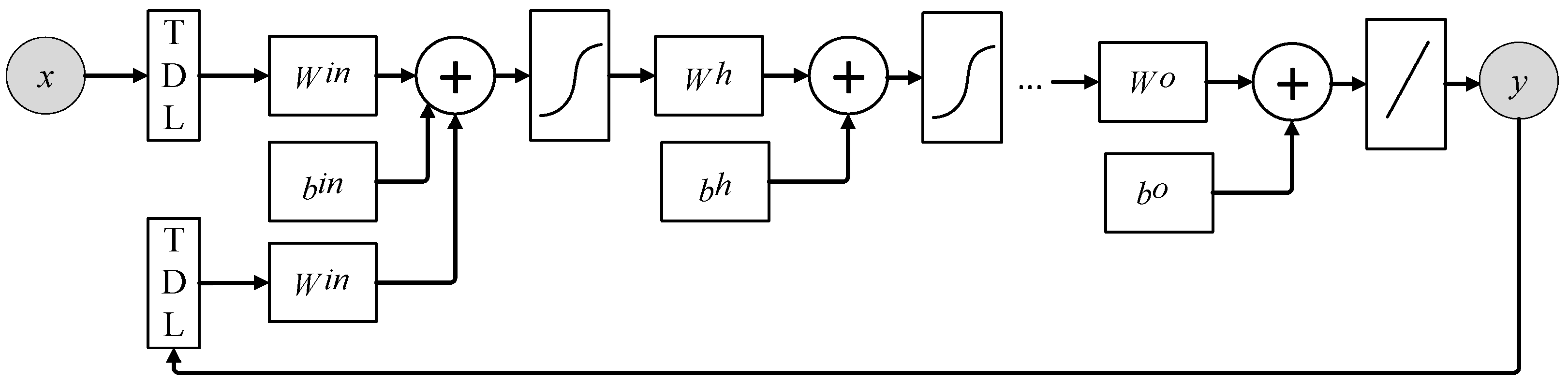
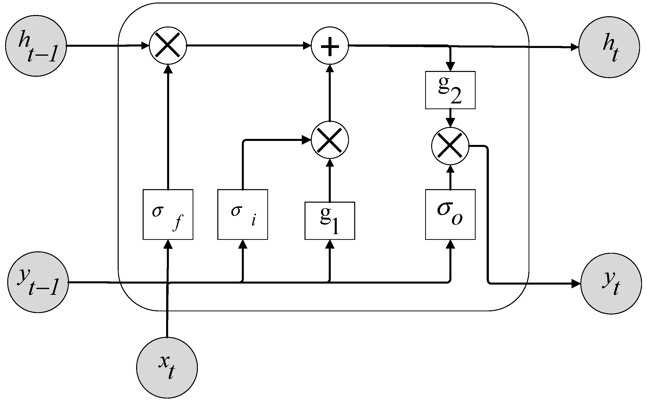
Some studies have shown that the NARX also suffers from the vanishing gradient problem [46,56], but in our study, the NARX outperformed ERNN and ESN. We also found that the NARX performed much better than other conventional RNNs in simulating basin hydrology. It is easier to discover long-term dependencies with the gradient descent of the NARX architecture than with other RNN architectures without output delays [41,42,57], maybe because long-term dependencies are influenced by the output delays. As illustrated in Figure A3 which shows the unfolded NARX architecture, the output delays (TDL in the figure) are manifested as jump-ahead connections in the unfolded network, and these jump-ahead connections provided a shorter path for propagating gradient information, which reduced the sensitivity to long-term dependencies. Besides, the output delays are passing ahead together without propagating through nonlinear hidden layers at every time step. This makes the gradient avoid degradation due to the partial derivative of the nonlinearity at every time step [44,57]. The performance of the LSTM is equivalent to that of the NARX in predicting discharges, since the LSTM architecture (Figure A4) facilitates the gradient information flows by adding a path in the cell between adjacent time steps and by adding gates, which controls whether the cell remembers or forgets certain information. Thus, the LSTM also addresses the long-term dependency problem, but by using a different mechanism.

5. Conclusions

This study compared the performance of the GR4J model and four recurrent neural networks in predicting the streamflow for two basins in China. The LSTM and NARX networks outperformed the ERNN and ESN networks. Hybrid models (GR4J with LSTM and GR4J with NARX) were developed to improve the accuracy of the discharge forecasting. In addition, the uncertainties of high, median, and low flows from the hybrid models were analyzed in comparison with flows from the single hydrological model.

The selection of a suitable RNN architecture is critical in simulating basin hydrology. RNNs with more complex architecture, which can accommodate long-term dependency, such as the LSTM and NARX, can better capture time-series dynamics and exhibit more promising ability in predicting streamflow than simpler RNNs. The models showed consistent results for the two basins, and the GR4J model with both LSTM and NARX performed better for the smaller catchment, which had less drainage area, smaller peak flows, and less time-series variation. However, LSTM and NARX were less variable, since the differences in measurement indicators (NSE, RMSE, and MAPE) were less for different basins.

More accurate streamflow forecasting for both basins were given by integrating the hydrological model with the RNNs (hybrid models GL and GN) than a single hydrological model or an RNN alone. The integrated models also provided better estimates of high, median, and low flows in both basins. Underestimation of the high flows with GR4J was reduced by 50% with GN and GL. If measured with relative percentage, low-flows errors reduced by 66% with GN and 63% with GL for the Xiangjiang River basin.

The uncertainty intervals of the median and low flows in the two basins predicted by both GN and GL were reduced by >50%. The GN model also increased the cover ratios in most cases, particularly for the high and low-flow forecasting. The GL model reduced the range of the uncertainty interval for the Qujiang basin more than the GN model, but this was accompanied by a reduction of the cover ratio.

References

- Beven, K. So how much of your error is epistemic? Lessons from Japan and Italy. Hydrol. Process. 2013, 27, 1677–1680. [Google Scholar] [CrossRef]
- Beven, K. Facets of uncertainty: Epistemic uncertainty, non-stationarity, likelihood, hypothesis testing, and communication. Int. Assoc. Sci. Hydrol. Bull. 2016, 61, 1652–1665. [Google Scholar] [CrossRef]
- Fraedrich, K.; Morison, R.; Leslie, L.M. Improved tropical cyclone track predictions using error recycling. Meteorol. Atmos. Phys. 2000, 74, 51–56. [Google Scholar] [CrossRef]
- Xiong, L.; O’Connor, K. Comparison of four updating models for real-time river flow forecasting. Int. Assoc. Sci. Hydrol. Bull. 2002, 47, 621–639. [Google Scholar] [CrossRef] [Green Version]
- Chen, L.; Zhang, Y.; Zhou, J.; Singh, V.P.; Guo, S.; Zhang, J. Real-time error correction method combined with combination flood forecasting technique for improving the accuracy of flood forecasting. J. Hydrol. 2015, 521, 157–169. [Google Scholar] [CrossRef]
- Yen, H.; Wang, X.; Fontane, D.G.; Harmel, R.D.; Arabi, M. A framework for propagation of uncertainty contributed by parameterization, input data, model structure, and calibration/validation data in watershed modeling. Environ. Model. Softw. 2014, 54, 211–221. [Google Scholar] [CrossRef]
- Whitfield, P.H.; Wang, J.Y.; Cannon, A.J. Modelling future streamflow extremes—Floods and low flows in Georgia Basin, British Columbia. Can. Water Resour. J. 2003, 28, 633–656. [Google Scholar] [CrossRef]
- Collet, L.; Beevers, L.; Prudhomme, C. Assessing the impact of climate change and extreme value uncertainty to extreme flows across Great Britain. Water 2017, 9, 103. [Google Scholar] [CrossRef]
- Marshall, L.; Nott, D.; Sharma, A. A comparative study of Markov chain Monte Carlo methods for conceptual rainfall-runoff modeling. Water Resour. Res. 2004, 40, 183–188. [Google Scholar] [CrossRef]
- Raje, D.; Krishnan, R. Bayesian parameter uncertainty modeling in a macroscale hydrologic model and its impact on Indian river basin hydrology under climate change. Water Resour. Res. 2012, 48, 2838–2844. [Google Scholar] [CrossRef]
- Yang, J.; Reichert, P.; Abbaspour, K.C. Bayesian uncertainty analysis in distributed hydrologic modeling: A case study in the Thur River basin (Switzerland). Water Resour. Res. 2007, 43, 145–151. [Google Scholar] [CrossRef]
- Beven, K.; Binley, A. The future of distributed models: Model calibration and uncertainty prediction. Hydrol. Process. 1992, 6, 279–298. [Google Scholar] [CrossRef]
- McMichael, C.E.; Hope, A.S.; Loaiciga, H.A. Distributed hydrological modeling in California semi-arid shrublands: MIKESHE model calibration and uncertainty estimation. J. Hydrol. 2006, 317, 307–324. [Google Scholar] [CrossRef]
- Mirzaei, M.; Galavi, H.; Faghih, M.; Huang, Y.F.; Lee, T.S.; El-Shafie, A. Model calibration and uncertainty analysis of runoff in the Zayanderood River basin using Generalized Likelihood Uncertainty Estimation (GLUE) method. J. Water Supply Res. Technol. 2013, 62, 309–320. [Google Scholar] [CrossRef]
- Rigon, R.; Bertoldi, G.; Over, T.M. GEOtop: A distributed hydrological model with coupled water and energy budgets. J. Hydrometeorol. 2006, 7, 371–388. [Google Scholar] [CrossRef]
- Güntner, A. Improvement of global hydrological models using GRACE data. Surv. Geophys. 2008, 29, 375–397. [Google Scholar] [CrossRef]
- Liu, Y.; Wang, W.; Hu, Y.; Cui, W. Improving the Distributed Hydrological Model Performance in Upper Huai River basin: Using streamflow observations to update the basin states via the Ensemble Kalman Filter. Adv. Meteorol. 2016, 2016, 4921616. [Google Scholar] [CrossRef]
- Paturel, J.E.; Mahé, G.; Diello, P.; Barbier, B.; Dezetter, A.; Dieulin, C.; Karambiri, H.; Yacouba, H.; Maiga, A. Using land cover changes and demographic data to improve hydrological modeling in the Sahel. Hydrol. Process. 2016, 31, 811–824. [Google Scholar] [CrossRef] [Green Version]
- Wu, S.J.; Lien, H.C.; Chang, C.H.; Shen, J.C. Real-time correction of water stage forecast during rainstorm events using combination of forecast errors. Stoch. Env. Res. Risk Assess. 2012, 26, 519–531. [Google Scholar] [CrossRef]
- Hsu, K.; Gupta, H.V.; Sorooshian, S. Artificial neural network modeling of the rainfall-runoff process. Water Resour. Res. 1995, 31, 2517–2530. [Google Scholar] [CrossRef]
- Lee, J.; Kim, C.-G.; Lee, J.; Kim, N.; Kim, H. Application of artificial neural networks to rainfall forecasting in the Geum River basin, Korea. Water 2018, 10, 1448. [Google Scholar] [CrossRef]
- Wu, C.L.; Chau, K.W.; Li, Y.S. River stage prediction based on a distributed support vector regression. J. Hydrol. 2008, 358, 96–111. [Google Scholar] [CrossRef] [Green Version]
- Belayneh, A.; Adamowski, J.; Khalil, B.; Ozga-Zielinski, B. Long-term SPI drought forecasting in the Awash River Basin in Ethiopia using wavelet neural network and wavelet support vector regression models. J. Hydrol. 2014, 508, 418–429. [Google Scholar] [CrossRef]
- Humphrey, G.B.; Gibbs, M.S.; Dandy, G.C.; Maier, H.R. A hybrid approach to monthly streamflow forecasting: Integrating hydrological model outputs into a Bayesian artificial neural network. J. Hydrol. 2016, 540, 623–640. [Google Scholar] [CrossRef]
- Shiau, J.T.; Hsu, H.T. Suitability of ANN-Based Daily Streamflow extension models: A case study of Gaoping River basin, Taiwan. Water Resour. Manag. 2016, 30, 1499–1513. [Google Scholar] [CrossRef]
- Sahoo, S.; Russo, T.A.; Elliott, J.; Foster, I. Machine learning algorithms for modeling groundwater level changes in agricultural regions of the U.S. Water Resour. Res. 2017, 53, 3878–3895. [Google Scholar] [CrossRef]
- Chang, F.J.; Lo, Y.C.; Chen, P.A.; Chang, L.C.; Shieh, M.C. Multi-Step-Ahead Reservoir Inflow Forecasting by Artificial Intelligence Techniques; Springer International Publishing: Cham, Switzerland, 2015; pp. 235–249. [Google Scholar]
- Lipton, Z.C.; Berkowitz, J.; Elkan, C. A Critical Review of Recurrent Neural Networks for Sequence Learning. Computer Science. arXiv, 2015; arXiv:1506.00019. [Google Scholar]
- Jiang, C.; Chen, S.; Chen, Y.; Zhang, B.; Feng, Z.; Zhou, H.; Bo, Y. A MEMS IMU De-Noising method using long short term memory recurrent neural networks (LSTM-RNN). Sensors 2018, 18, 3470. [Google Scholar] [CrossRef] [PubMed]
- Chang, F.J.; Chen, P.A.; Lu, Y.R.; Huang, E.; Chang, K.Y. Real-time multi-step-ahead water level forecasting by recurrent neural networks for urban flood control. J. Hydrol. 2014, 517, 836–846. [Google Scholar] [CrossRef]
- Chen, P.A.; Chang, L.C.; Chang, F.J. Reinforced recurrent neural networks for multi-step-ahead flood forecasts. J. Hydrol. 2013, 497, 71–79. [Google Scholar] [CrossRef]
- Shen, H.Y.; Chang, L.C. Online multistep-ahead inundation depth forecasts by recurrent NARX networks. Hydrol. Earth Syst. Sci. 2013, 17, 935–945. [Google Scholar] [CrossRef] [Green Version]
- Liang, C.; Li, H.; Lei, M.; Du, Q. Dongting Lake Water Level Forecast and Its Relationship with the Three Gorges Dam Based on a Long Short-Term Memory Network. Water 2018, 10, 1389. [Google Scholar]
- Perrin, C.; Michel, C.; Andréassian, V. Improvement of a parsimonious model for streamflow simulation. J. Hydrol. 2003, 279, 275–289. [Google Scholar] [CrossRef]
- Thyer, M.; Renard, B.; Kavetski, D.; Kuczera, G.; Franks, S.W.; Srikanthan, S. Critical evaluation of parameter consistency and predictive uncertainty in hydrological modeling: A case study using Bayesian total error analysis. Water Resour. Res. 2009, 45, 1211–1236. [Google Scholar] [CrossRef]
- Elman, J.L. Finding structure in time. Cogn. Sci. 1990, 14, 179–211. [Google Scholar] [CrossRef]
- Demuth, H.; Beale, M. Neural Network Toolbox for Use with MATLAB. User’s Guide Version 4. 2002. Available online: http://www.image.ece.ntua.gr/courses_static/nn/matlab/nnet.pdf (accessed on 13 November 2018).
- Jaeger, H. Adaptive Nonlinear System Identification with Echo State Networks. In Proceedings of the NIPS’02 15th International Conference on Neural Information Processing Systems, Vancouver, BC, Canada, 9–14 December 2002; pp. 609–616. [Google Scholar]
- Jaeger, H.; Lukosevicius, M.; Popovici, D.; Siewert, U. Optimization and applications of echo state networks with leaky-integrator neurons. Neural Netw. 2007, 20, 335–352. [Google Scholar] [CrossRef] [PubMed]
- Leontaritis, I.J.; Billings, S.A. Input-output parametric models for non-linear systems Part I: Deterministic non-linear systems. Int. J. Control 1985, 41, 303–328. [Google Scholar] [CrossRef]
- Horne, B.G. An experimental comparison of recurrent neural networks. Adv. Neural Inf. Process. Syst. 1995, 7, 697–704. [Google Scholar]
- Menezes, J.; Maria, P.; Barreto, G.A. Long-term time series prediction with the NARX network: An empirical evaluation. Neurocomputing 2008, 71, 3335–3343. [Google Scholar] [CrossRef]
- Marquardt, D.W. An algorithm for least-squares estimation of nonlinear parameters. Soc. Ind. Appl. Math. 1963, 11, 431–441. [Google Scholar]
- Dipietro, R.; Rupprecht, C.; Navab, N.; Hager, G.D. Analyzing and Exploiting NARX recurrent neural networks for long-term dependencies. arXiv, 2017; arXiv:1702.07805. [Google Scholar]
- Hochreiter, S.; Schmidhuber, J. Long short-term memory. Neural Comput. 1997, 9, 1735–1780. [Google Scholar] [CrossRef] [PubMed]
- Gers, F. Long Short-Term Memory in Recurrent Neural Networks; University of Hannover: Hannover, Germany, 2001. [Google Scholar]
- Gers, F.A.; Schmidhuber, J.A.; Cummins, F.A. Learning to forget: Continual prediction with LSTM. In Proceedings of the Ninth International Conference on Artificial Neural Networks, ICANN 99, Edinburgh, UK, 7–10 September 1999; p. 2451. [Google Scholar]
- Graves, A. Supervised Sequence Labelling with Recurrent Neural Networks; Springer: Berlin/Heidelberg, Germany, 2012. [Google Scholar]
- Li, X.; Peng, L.; Yao, X.; Cui, S.; Hu, Y.; You, C.; Chi, T. Long short-term memory neural network for air pollutant concentration predictions: Method development and evaluation. Environ. Pollut. 2017, 231, 997–1004. [Google Scholar] [CrossRef] [PubMed]
- Zhang, D.; Lindholm, G.; Ratnaweera, H. Use long short-term memory to enhance Internet of Things for combined sewer overflow monitoring. J. Hydrol. 2018, 556, 409–418. [Google Scholar] [CrossRef]
- Kratzert, F.; Klotz, D.; Brenner, C.; Schulz, K.; Herrnegger, M. Rainfall-Runoff modelling using Long-Short-Term-Memory (LSTM) networks. Hydrol. Earth Syst. Sci. Discuss. 2018. [Google Scholar] [CrossRef]
- Beven, K. A manifesto for the equifinality thesis. J. Hydrol. 2006, 320, 18–36. [Google Scholar] [CrossRef] [Green Version]
- Shin, M.J.; Kim, C.S. Assessment of the suitability of rainfall-runoff models by coupling performance statistics and sensitivity analysis. Hydrol. Res. 2017. [Google Scholar] [CrossRef]
- Tian, Y.; Xu, Y.P.; Booij, M.J.; Wang, G. Uncertainty in future high flows in Qiantang River Basin, China. J. Hydrometeorol. 2015, 16, 363–380. [Google Scholar] [CrossRef]
- Jaeger, H. The Echo State Approach to Analysing and Training Recurrent Neural Networks; GMD Report 148; German National Research Center for Information Technology: Bonn, Germany, 2001. [Google Scholar]
- Diaconescu, E. The use of NARX neural networks to predict chaotic time series. WSEAS Trans. Comp. Res. 2008, 3, 182–191. [Google Scholar]
- Lin, T.; Horne, B.G.; Tiňo, P.; Giles, C.L. Learning long-term dependencies in NARX recurrent neural networks. IEEE Trans. Neural Netw. 1996, 7, 1329–1338. [Google Scholar] [CrossRef] [PubMed] [Green Version]
Figure 1.
Location of the study areas and observation stations.
Figure 2.
Errors in predicted discharge versus observation given by GR4J, nonlinear autoregressive exogenous inputs neural network (NARX), and long short-term memory (LSTM) for the Xiangjiang and Qujiang basins.
Figure 3.
Comparison of daily discharge forecasting for the Xiangjiang (upper) and Qujiang (lower) basins between GR4J and the GR4J hydrological model integrated with LSTM (GL) (above) and GR4J and the GR4J hydrological model integrated with NARX (GN) (below).
Figure 4.
Ranges of forecasting errors in high, medium, and low flows in the Xiangjiang and Quajiang River basins.
Figure 5.
NSE values for GR4J, GN, and GL in the Xiangjiang and Qujiang basins.
Figure 6.
Uncertainty intervals of Qmax, Qmed, and Q95 in the years 1981–1995 for GR4J, GN, and GL in the Xiangjiang and Qujiang basins.