Article

Assessing the Importance of Potholes in the Canadian Prairie Region under Future Climate Change Scenarios

1
Department of Civil Engineering, University of Manitoba, Winnipeg, MB R3T 5V6, Canada
2
Deportment of Water Environment, Agricultural and Biological Engineering, The Ohio State University, Columbus, OH 43210, USA
3
Department of Soils, Water & Agricultural Engineering College of Agricultural & Marine Sciences Sultan Qaboos University, P.O. Box 34, Al-Khod 123, Oman
4
Earth and Environmental Sciences, Indian Institute of Science Education and Research Bhopal, Bhopal, Bhauri Bypass Road, Bhauri, Bhopal 462066, Madhya Pradesh, India
5
Department of Civil Engineering, McMaster University, Hamilton, ON L8S 4L7, Canada
*
Author to whom correspondence should be addressed.
Water 2018, 10(11), 1657; https://doi.org/10.3390/w10111657
Submission received: 20 October 2018 / Revised: 12 November 2018 / Accepted: 12 November 2018 / Published: 14 November 2018
(This article belongs to the Special Issue Catchment Modelling)

Abstract

:
The Prairie Pothole Region (PPR) of Canada contains millions of small isolated wetlands and is unique to North America. The goods and services of these isolated wetlands are highly sensitive to variations in precipitation and temperature. We evaluated the flood proofing of isolated wetlands (pothole wetlands) under various climate change scenarios in the Upper Assiniboine River Basin (UARB) at Kamsack, a headwater catchment of the Lake of the Prairies in the Canadian portion of the PPR. A modified version of the Soil Water Assessment Tool (SWAT) model was utilized to simulate projected streamflow under the potential impacts of climate change, along with changes to the distribution of pothole wetlands. Significant increases in winter streamflow (~200%) and decreases (~11%) in summer flow, driven by changes in future climates, were simulated. Simulated changes in streamflow resulting from pothole removal were between 55% for winter and 15% for summer, suggesting that climate will be the primary driver in the future hydrologic regime of the study region. This research serves as an important guide to the various stakeholder organizations involved in quantifying the aggregate impacts of pothole wetlands in the hydrology of the Canadian Prairie Region.

1. Introduction

The North American Prairie Pothole Region (PPR) spans across Alberta, Saskatchewan, and Manitoba in Canada and extends into North Dakota, South Dakota, Iowa, Minnesota, and Montana in the United States (US) (Figure 1). The PPR is home to millions of isolated wetlands (i.e., pothole wetlands) that provide a range of ecosystem goods and services such as flood attenuation, groundwater recharge, biogeochemical processing, and regional diversity [1,2,3,4,5,6]. Despite the numerous benefits, nearly 70% of the wetlands have been lost in the PPR, with 84% of this loss attributed to agricultural development [6,7].
Wetlands play a major role in watershed health [8,9,10,11] and can be seen as an integral component of much of the prairie landscape. Wetlands help to mitigate the effects of climate change by reducing the effects of drought and inundation. During wetter periods, they store a large amount of water, helping to reduce peak flood flows. In dry periods, they retain water, helping to recharge groundwater [12,13,14]. Wetlands, however, due to their shallow nature, are highly susceptible to changes in climate and land use [4,7,15]. The Intergovernmental Panel on Climate change (IPCC), in its fifth assessment report, projected a 2–5 °C rise in the surface temperature [16,17]. Consequently, it is very likely that extreme precipitation events will become more intense and frequent, altering the hydrologic cycle and water availability in many regions [18,19].
Global Circulation Models (GCMs) have been considered effective tools in exploring the physical processes of the earth’s surface atmospheric system and are widely utilized to gain information regarding historical, current, and future climates [20]. Based on estimates of future population levels, economic activity, and technological patterns [16,21,22], the future climate change scenarios from GCMs are used to assess future vulnerability attributed to climate change [23]. Numerous studies have suggested that climate change may have a far more significant impact on the PPR of North America, where runoff is mainly driven by seasonal snowmelt [24,25,26,27,28]. Most regions of the Canadian Prairie Pothole Region (CPPR) are projected to warm over the next 60 years [29], in particular the central CPPR, where warming is expected to be more pronounced [30], thus potentially resulting in increased drought and excessive moisture risk [31]. For example, snowfall in the CPPR accounts for about 30% of total annual precipitation and produces 80% or more of the total annual surface runoff [32,33]. Changes in the amount and seasonality of air temperatures and precipitation could significantly alter the volume, distribution, and timing of snowfall, which may affect the hydrology of the prairie.
While it is essential to consider the potential effects of climate change, several studies have also highlighted the significance of land use change and its vital role in the hydrology of the CPPR [6,15,34,35,36]. For example, the loss of wetland surface runoff in the prairie often drains into depressions, forming wetlands or pothole wetlands. Pothole wetlands are closed basins that retain water for a longer duration due to their higher retention capacity [12,37,38,39], and do not contribute flow to streams under normal condition. However, during times of high runoff, pothole wetlands connect to each other and to streams via a fill-and-spill process [40], which results in a dynamic increase in the contributing area for runoff to streams [13,15]. Land use changes, in particular the loss of pothole wetlands mainly due to agricultural development, greatly alter hydrological processes, affecting both water quality and quantity. Thus, there is a pressing need to thoroughly investigate the coupled effect of climate and land use change on the hydrology of the CPPR.
Watershed-scale hydrologic models can be valuable tools that enhance our understanding of complex natural processes and aid in examining land use change and best management practices (BMPs). Advances in computational resources have further enhanced modeling at finer-scale resolutions while discretizing the geospatial heterogeneity of a watershed. The Soil Water Assessment Tool (SWAT) is a watershed-scale model that has been widely used for water resources assessment [41,42,43,44], climate and land use changes [45,46,47,48,49], water quality, pollutants and nutrients loading [50,51,52,53], and watershed management practices [54,55,56]. Hydrologic models constructed to study PPR watersheds must pay close attention to the important role that pothole wetlands play in the PPR hydrologic cycle.
The SWAT model has been utilized for studying climate-induced changes in hydrology and nutrient fluxes of the Upper Assiniboine River Basin (UARB) [57]. The study, however, did not explore land use as a factor—along with climate change—affecting hydrology. References [58,59] examined uncertainty in hydrological responses due to climate change in the Assiniboia watershed of Saskatchewan, Canada, using the SWAT model. A few other studies [34,60,61,62] used the SWAT model for investigating the impact of pothole wetlands on downstream hydrographs without considering the effects of climate change.
Given the importance of pothole wetlands to ecological goods and services, especially flood mitigation, there is a need for more research on the coupled impacts of climate and land use change. The primary focus of this research is to present an analysis of the compounding effects of climate and land use change on streamflow in the CPPR. Our method of land use change involved removal of pothole wetlands from the land surface. Our specific interests were to (1) examine the hydrological response at the outlet resulting from changes in both land use and climate change, and to (2) evaluate the effects on hydrograph sensitivity due to pothole wetland removal for extreme events. This research provides quantitative information for water managers and stakeholders in the PPR regarding the importance and significance of pothole wetlands in controlling the future PPR runoff response.

2. Materials and Methods
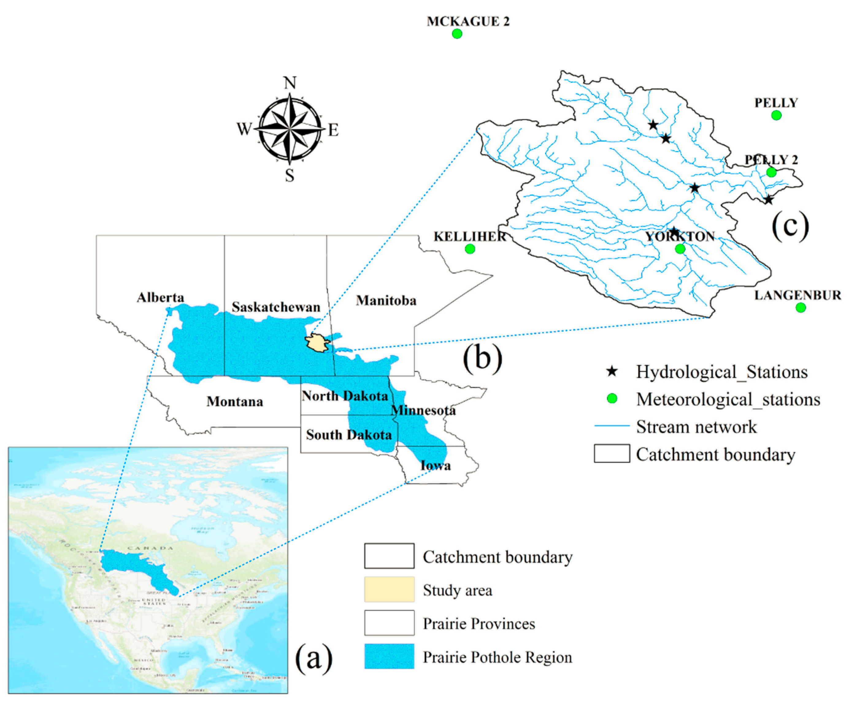
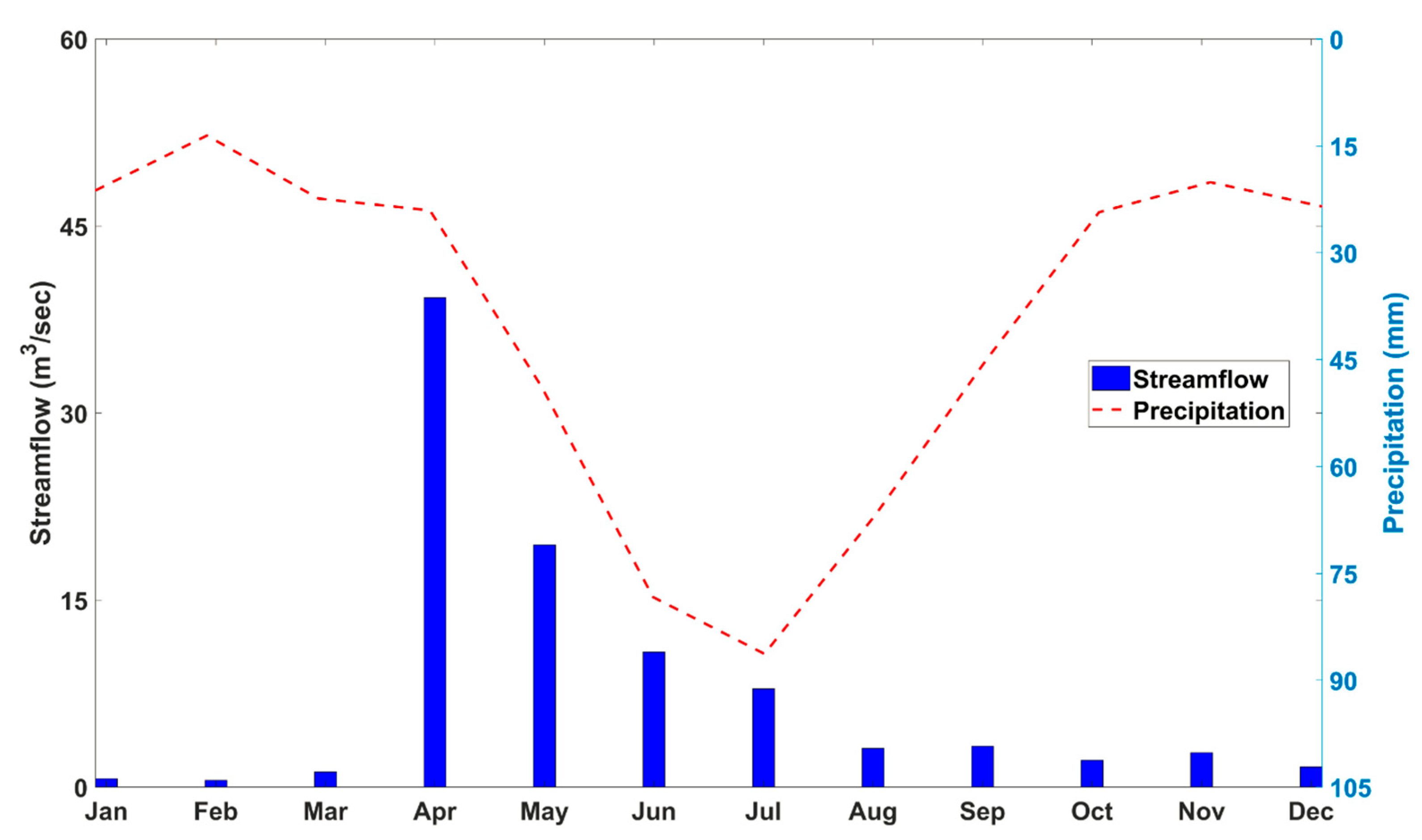
2.1. Study Area

The presence of potholes that create intermittent flow, the existence of numerous lakes, and the dynamics of the wetlands are defining characteristics of the UARB at Kamsack. Spanning the provinces of Saskatchewan and Manitoba, the UARB has a total area of 13,000 km2 and is monitored by five streamflow gauging stations (Figure 1c). The basin is of vital importance, as flow generated in the basin enters the Lake of the Prairies (the Shellmouth Reservoir), which was constructed for flood mitigation purposes and is situated approximately 45 km downstream of the watershed outlet. The Manitoba Hydrologic Forecasting Centre (HFC) has a deep interest in the basin, as the volume of water that generates in the basin directly flows into the Shellmouth Reservoir, for which HFC is tasked to set operating rules. Knowing the long-term climate and land use change impact on the hydrology of the basin, the HFC will be better able to prepare water resource planning and management operations.
The climate of the UARB is continental subhumid characterized by long, cold winters and short summers, where the mean annual temperature and potential evapotranspiration is about 1 °C and 850 mm, respectively [63]. Average annual precipitation is 450 mm, with approximately 26% of the precipitation falling as snow [57]. Spring freshet occurs from April to June, accounting for 82%, on average, of total mean annual streamflow [57] (Figure 2).
Black Chernozemic soils overlay almost 70% of the basin: They are high in organic matter and have generally developed under native grassland [64]. A detailed literature review and investigation that highlights the distribution of wetland soils in the PPR was presented in Reference [65], whereas Reference [66] presented a discussion on the types and presence of wetlands in the PPR and what impacts they may have on ecohydrology.

2.2. Geospatial and Hydroclimatic Data

SWAT requires climate data, topography, land use, and soil type as inputs. Climate data at a daily time step for the period 1981–2015 were obtained from Environment and Climate Change Canada (ECCC). Six meteorological stations were considered, of which two resided within the basin and four were nearby (Figure 1c). A digital elevation model (DEM) using 20 m spatial resolution [67] and 30 m spatial resolution land use data [68] were obtained from the GeoGratis Data Portal (http://geogratis.gc.ca/). Detailed soil data were obtained from Agriculture and Agri-Food Canada’s Manitoba regional office. These data were of 30 m spatial resolution with information for up to six layers of soil depth at 5, 15, 30, 60, 100, and 200 cm. The observed daily streamflow time series, which was required for model calibration and validation, was obtained from ECCC’s Water Survey of Canada (WSC) hydrometric database (HYDAT) (Table 1).

2.3. Hydrological Model

This study utilized the modified version of the SWAT (ver. 2012 rev. 627) model. Potholes in the SWAT are defined at the Hydrologic Response Unit (HRU) level. The standard version of the SWAT does not recognize the hydrologic relationship of pothole wetlands to uplands and other upgradient pothole wetlands. For instance, in the prairie region, the upgradient drainage area of a pothole may stretch out past the limits of its particular HRU and would receive inflow from numerous upgradient HRUs. The SWAT does not mimic between pothole fill-and-spill connections in light of the fact that hydrologic transport between HRUs is unrealistic inside the model [69]. Consequently, a new geographically isolated wetlands (GIWs) module was added to the model to simulate GIWs (i.e., potholes). However, modifications were also made to a number of other modules to facilitate simulation of fill-and-spill processes (e.g., where upgradient HRUs drain to downgradient pothole HRUs, and pothole HRUs fill to capacity and spill to a downgradient pothole HRU). Additional information regarding model modification was provided by Reference [70]. The modified version, which has enhanced representation of pothole wetlands, was able to better adapt to the physical processes that occurred in our study watershed.

2.4. Calibration and Validation

The Sequential Uncertainty Fitting version 2 (SUFI-2) was used as a mean of calibrating and validating the model. SUFI-2 is programmed in the SWAT-Calibration and Uncertainty Program (SWAT-CUP), which is a module developed to automate calibration [71]. In SUFI-2, parameter uncertainty is described by a multivariate uniform distribution, which is expressed in ranges, while output uncertainty is described by the 95% prediction uncertainty band (95PPU). The 95PPU is calculated at the 2.5% and 97.5% levels of the cumulative distribution function (CDF) for the output variables [51,72]. Latin hypercube sampling is used to draw independent parameter sets [51]. The goodness of fit during calibration and prediction uncertainty are evaluated based on the closeness of the p-factor to 100% (i.e., all observations fall within the 95PPU) and the r-factor to 0 (i.e., the width of the 95PPU). Reference [73] suggested that p-factor values above 0.7 and r-factor values below 1.5 are satisfactory.
In this study, the model was calibrated for the period 1981–2010 and verified from 2011–2015, considering all flow gauging stations. The Kling–Gupta [74] efficiency (KGE) metric was used as a guide for selecting the most optimal parameters and for evaluating model performance (Equation (1)):
K G E = 1 ( r 1 ) 2 + ( 1 ) 2 + ( β 1 ) 2 ,
where α = σ s σ m , β = μ s μ m .
Here, σs and σm are the standard deviation of simulated and measured data, µs and µm are the means for simulated and measured data, respectively, and r is the linear regression coefficient between measured and simulated data. KGE allowed for a multi-objective perspective by focusing on correlation error, variability error, and bias (volume) error [75]. A KGE > 0.5, recommended by Reference [74], was set as the threshold value for selecting simulation runs while running the autocalibration program. Other performance metrics such as Nash–Sutcliffe efficiency (NSE) [76] and percent bias (PBIAS) [74,77] were also utilized to further assess model performance. In this paper, the model calibration effort should have satisfied the following criteria for satisfactory performance:
  • KGE ≥ 0.5, as recommended by Reference [74];
  • NSE ≥ 0.5, as recommended by Reference [78];
  • PBIAS ≤ ±0.25, as recommended by Reference [78]; and
  • p-factor ≥ 0.7 and r-factor ≤ 1.5, as suggested by Reference [73], for the 95% prediction uncertainty when using SUFI-2.

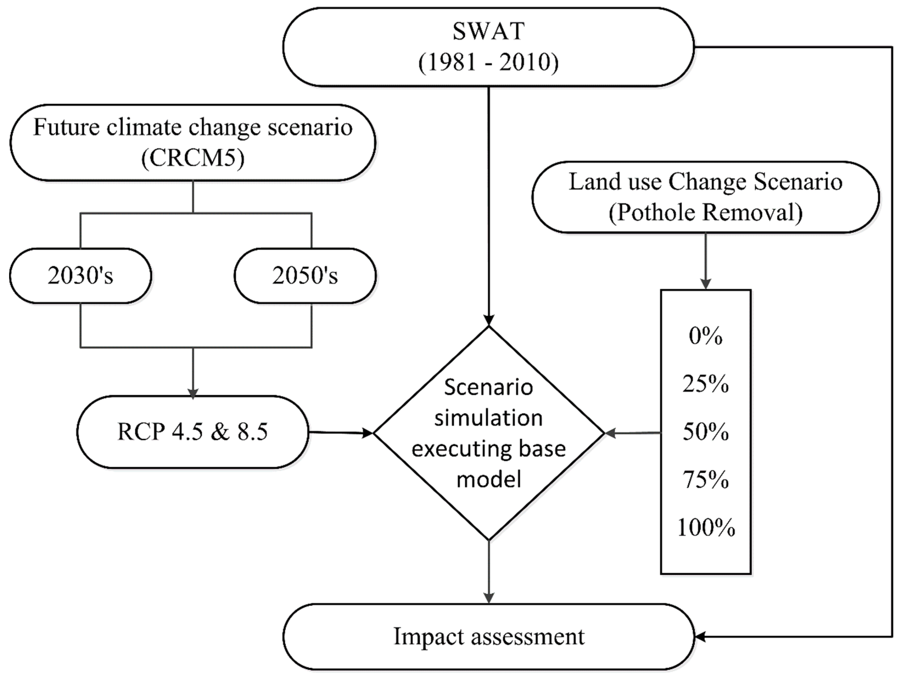
2.5. Scenario Formulation: Climate and Land Use Change

The Canadian Regional Climate Model (CRCM) version 5 was used to extract future climate data. It has a higher resolution than GCM data, is the most up-to-date CRCM, and has several improvements, such as an improved land surface scheme [79,80,81]. We selected Representative Concentration Pathways (RCPs) 4.5 and 8.5 and two future periods, near future (2030s: 2011–2040) and middle future (2050s: 2041–2070), in our study. RCP 4.5 represented a moderate population and economic growth, with an average of a 1.4 °C rise in temperature. RCP 8.5 portrayed rapid population growth with modest technological changes and relatively slow income growth, thus leading to increased greenhouse gas emissions, resulting in an average of about a 2.0 °C rise in temperature [17,82].
Output from RCMs is subject to systematic biases [83,84,85,86] that may potentially affect hydrological simulations [87]. Thus we bias-corrected these data before application in our hydrological model. Performance and effectiveness of bias-correction techniques is dependent on the study location [88]. We utilized a quantile-quantile (Q-Q) mapping approach [89] to bias-correct the RCM data used in our study based on recommendations from References [88,90]. Figure 3 presents basin-averaged RCM data before and after the application of our Q-Q mapping bias correction.
The land use scenarios were created by varying the percent of pothole wetland coverage in the watershed. We used five land use scenarios by randomly removing 0%, 25%, 50%, 75%, and 100% of pothole wetlands from the land surface.
The calibrated model as a baseline model was used to run the combination of land use and climate change scenarios to assess the effect on the downstream hydrograph (WSC ID: 05MD004). Figure 4 shows a schematic diagram outlining scenario formulation. The combination of four climate and five land use change scenarios resulted in a total of 20 coupled land use and climate change scenarios.

3. Results

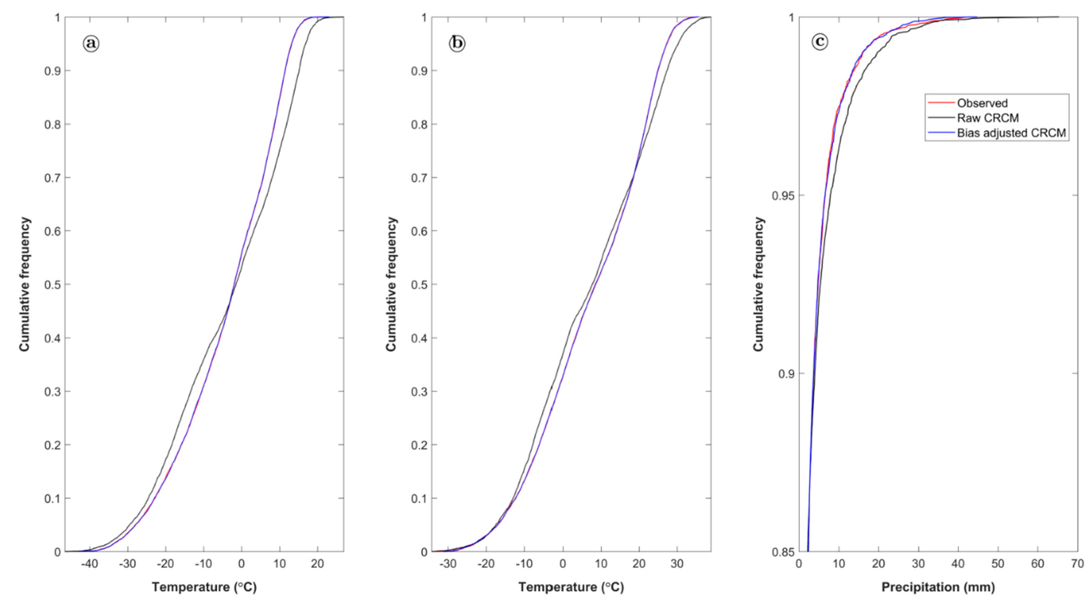
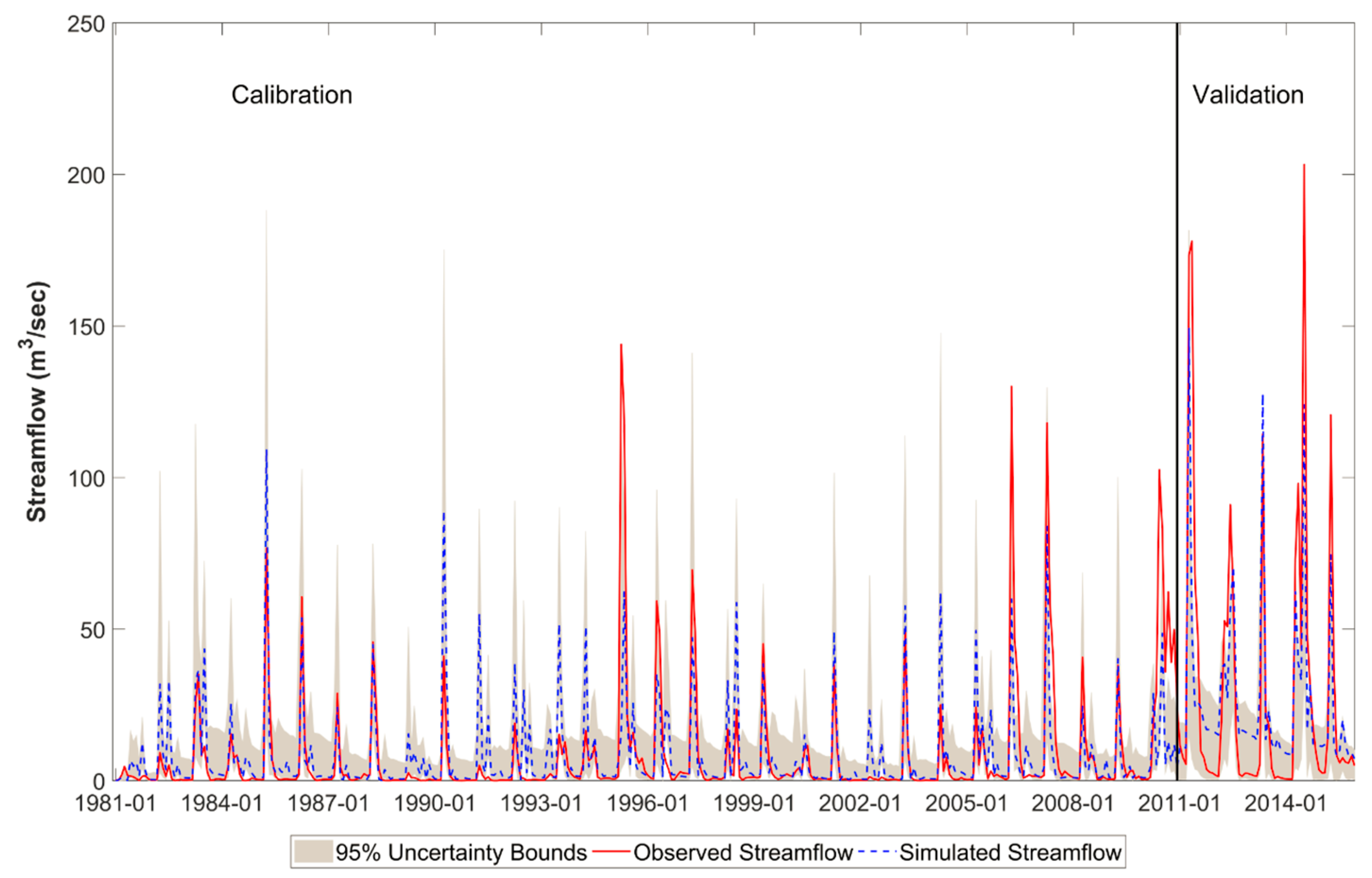
3.1. Model Calibration and Validation

For model calibration, key parameters that govern hydrologic processes of the study watershed were selected based on available literature [34,35,57,58,60,61,62,91,92,93]. A total of 27 parameters were considered in the calibration process. The minimum, maximum, and fitted values (Table 2) and observed and simulated hydrographs with 95% prediction uncertainty for the catchment outlet are presented (Figure 5).
In general, the model was able to capture the variability of streamflow, particularly the timing of the peak flow. In places, the model overestimated observed streamflow, such as during the years 1982–83, 1989, and in the spring of the year 2002, were dry years (relative to normal). During the validation period, low flows were overestimated and high flows underestimated. However, the model generally followed the seasonal patterning of streamflow. The p-factor and r-factor were within an acceptable range (Table 3). KGE, NSE, and PBIAS indicated satisfactory modeling results. All gauging stations listed in Table 3 were parameterized and optimized simultaneously. This may have led to some outlets being more poorly simulated than others, for example, at Ebenezer (WSC ID: 05MB001). In this case, the gauge was located downstream of approximately ten unregulated reservoirs, collectively known as the Yorkton complex, which significantly impacted the SWAT model performance due to the poor parameterization of reservoir releases.

3.2. Future Climate for the 2030s and 2050s Periods under RCP 4.5 and RCP 8.5 Scenarios

Figure 6 shows changes in the mean monthly (a) precipitation (mm) and (b) temperature (°C) for RCP 4.5 and 8.5 over two climatological periods centered around 2030 (2011–2040) and 2050 (2041–2070).
We used seasonal averages for ease of intercomparison. Our seasons were defined as winter (DJF), spring (MAM), summer (JJA), and fall (SON). There was a notable increase in winter precipitation, especially in December and January, under all climate projections. Precipitation decreased during summer, as also noted in Reference [94]. The climate model indicated an increase in temperature across the year for the basin. Increasing temperature, averaged across the basin, was more pronounced under RCP 8.5 (3.5 °C) compared to RCP 4.5 (2.5 °C) for the 2030s, but reversed by the 2050s (6 °C and 4.8 °C for RCP 4.5 and 8.5, respectively). Thus, it should not be assumed that the RCP 8.5 scenario represented the most extreme changes in climate for this region.

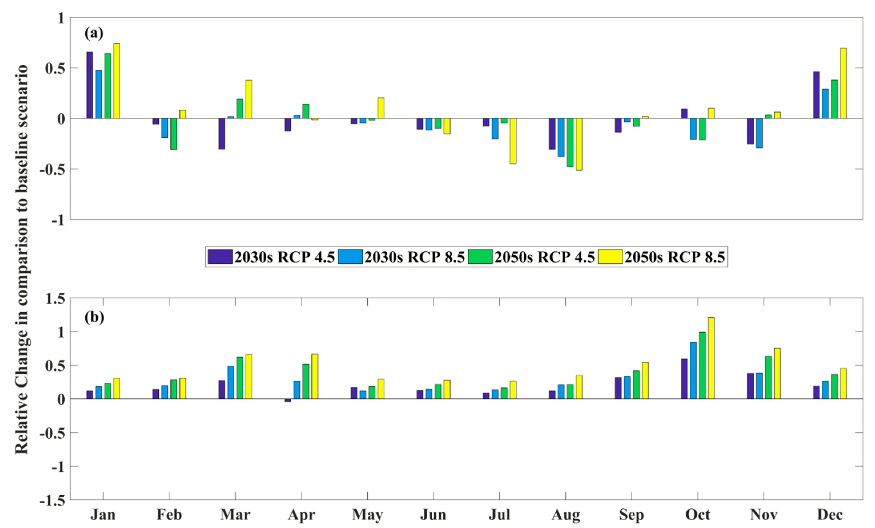
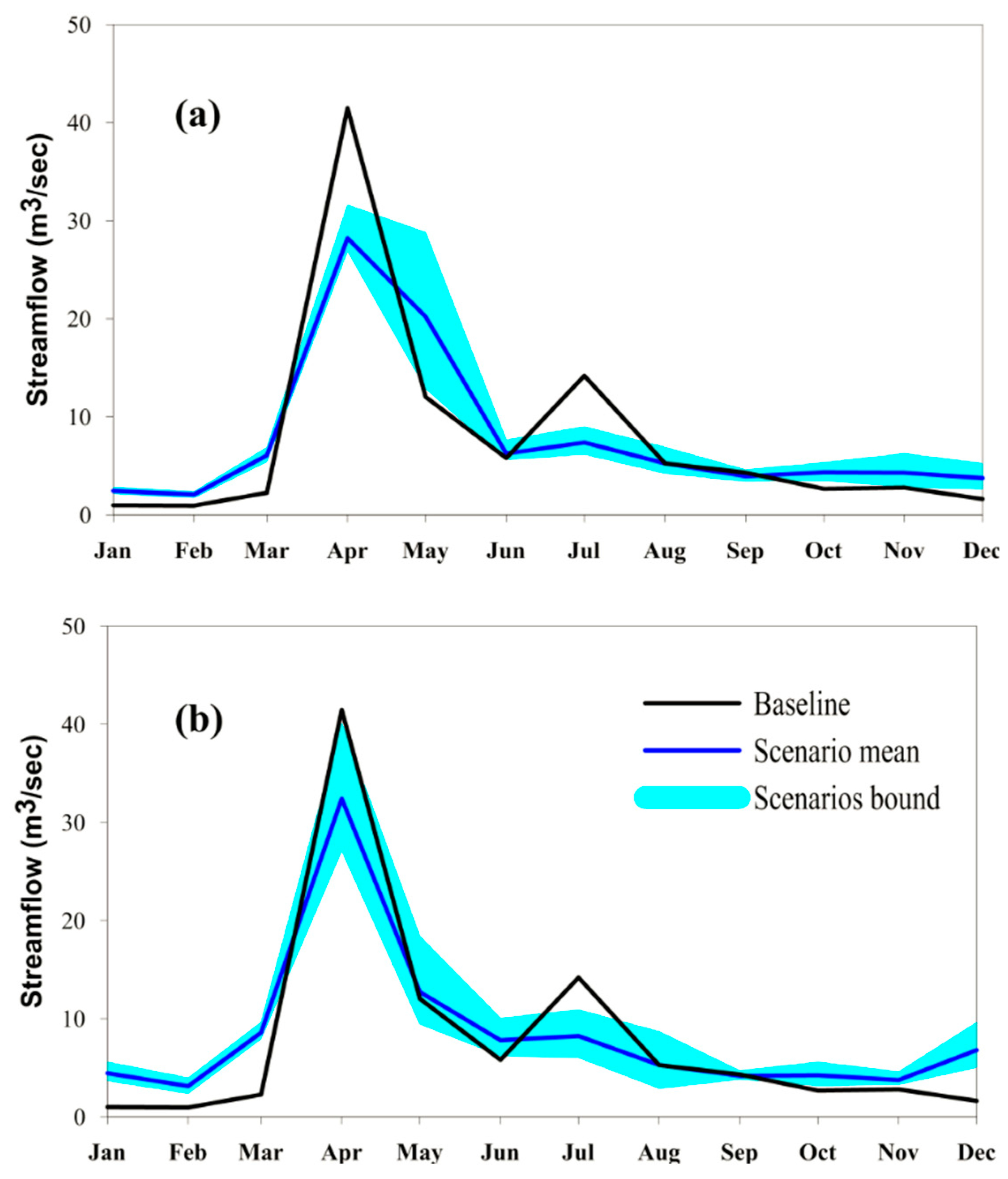
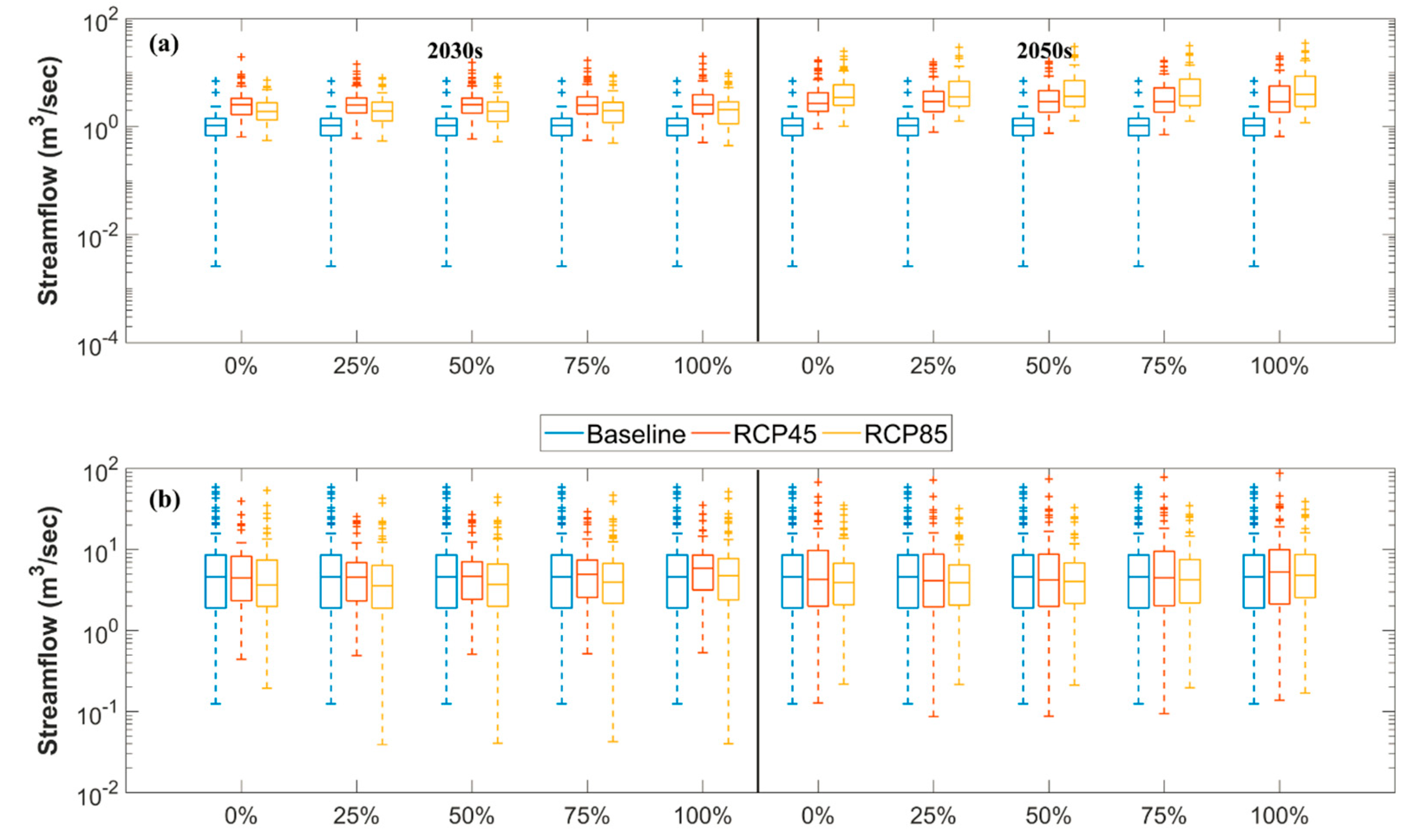
3.3. Variations in Streamflow

We began our evaluation by comparing future changes in the ensemble mean of all climate and land use change scenarios. Ensemble mean was used to reduce the uncertainty of future projections, primarily resulting from future climate. The mean monthly variation in streamflow response under climate and land use change for the two future time periods showed a significant increase in streamflow during winter, and decreases in spring peak discharge and summer streamflow across all scenarios (Figure 7). Such variations in streamflow were not unexpected for this region [95] and could be attributed to a shift toward wetter winters and drier summers. We, however, saw relatively high spring streamflow during the 2050s period in comparison to the 2030s period. This could be attributed to higher precipitation in the 2050s period.
To further investigate the coupled impact of land use and climate change, seasonal analyses were carried out. Changes in winter and summer streamflow were most notable (Figure 8). Median streamflow for winter was likely to increase (based on all climate scenarios, as seen in Figure 8), perhaps due to increasing precipitation falling as rain. Interestingly, increases from RCP 4.5 were relatively higher compared to RCP 8.5 for the 2030s. This could be linked to the climate data, where increasing precipitation for RCP 4.5 was observed compared to RCP 8.5 (Figure 6a).
The expansion of agriculturally dominated regions through pothole wetland removal further increased streamflow, indicating the sensitivity of streamflow to land use changes. For example, in comparison to the zero-removal scenario, a 30% increase in streamflow could be observed if all pothole wetlands were removed (Table 4) under the RCP 4.5 2030s period. The change under RCP 4.5 for the 2050s period could be up to a 65% increase in streamflow when all pothole wetlands were removed. A similar increasing pattern from the aforementioned future period was observed under RCP 8.5. For example, during the middle future, winter streamflow could nearly threefold with no land use change, up to a fourfold increase if all pothole wetlands were removed. Changes regarding percentage variation in summer streamflow were not as high in comparison to winter flows. For example, there was a 16% decrease in summer streamflow under RCP 4.5 with no wetland removal in comparison to a 160% increase in winter for the same period and scenario. Similarly, impact on streamflow variability between the two extreme land use scenarios during summer (~20%) was also lower in comparison to that during the winter season (~30%).
The flow duration curve for the baseline, extreme climate, and land use change scenarios, and the ensemble mean of the future scenarios (Figure 9), along with quantiles for 10%, 50%, and 90% exceedance probabilities (Table 5), are presented. A log10-normal probability curve for the extreme (high and low) of the combined land use and climate change, mean of the scenario, and baseline scenario were used to allow the low and high quantiles to be more visible. In general, we saw increasing flow in the near and middle futures in comparison to the baseline period. This means that, in the future, the probability of exceedance for low flow increased while the probability of exceedance for high flow decreased. Consequently, there would be a more frequent occurrence of low flow periods and less frequent high flow periods.
While the coupled impact of climate and land use change indicated overall increasing streamflow, there was a greater likelihood of lower high flows (relative to the baseline) based on Q10 (10% exceedance). Mean low flows in the future may have increased by up to 106% based on Q90 relative to the baseline period. Changes in the median quantile (i.e., Q50) suggested an increase of up to 180% over the baseline period (Table 5).

4. Discussion

Hydrology in the Canadian Prairie Region (CPR) is highly complex. Historically, only one-third of the precipitation occurs during winter, in the form of snow. However, snowmelt contributes approximately 80% of spring discharge. Both the timing and duration of seasonality are essential aspects of the CPPR climate. For the CPPR, variability in climate means changes in the distribution of solid and liquid precipitation, for example increased precipitation during winter (accumulated solid precipitation resulting in spring discharge) and decreased rainfall runoff during summer. Increasing precipitation coupled with a potential increase in temperature likely resulted in more precipitation falling as rain during the winter, or shoulder season, months, thus causing a shift toward earlier spring peak flow events (Figure 7). Consequently, this led to less water availability during summer and autumn when evaporative potential and agriculture demand was the highest. Dibike et al. (2012, 2017) also showed increasing water supply variability in the CPPR and, more specifically, decreased summer flows, where extreme deficits in water availability during summer months were projected.
Though climate warming is not uniformly projected across the globe, results for the CPPR indicate that warming (~6 °C rise by 2070 across the basin) may be more pronounced than the global average (~2–3 °C) for the same period. Previous studies [96,97,98] highlighted that rising temperatures would act as a catalyst in enhancing evapotranspiration, which has the potential to cause more water stress in summer. The combined effects of a water availability deficit, increasing temperatures, and increasing evapotranspiration suggest the potential for increasing frequency and severity of drought.
Our research indicated that the disappearance of isolated pothole wetlands played an equally critical role as the climate did in changing the hydrology of the CPPR. In our study, a 55% increase in winter streamflow was simulated for the 100% pothole removal scenario compared to our baseline scenario. Removing pothole wetlands could also potentially cause an increase in summer flow (~16%). Similar findings were observed by References [61,99] when isolated wetlands were fully drained.
All climate and land use change scenarios suggested an increase in low and median streamflow and a decrease in high flows (Figure 9), resulting in a more uniform streamflow behavior. The lack of variability in streamflow is often viewed negatively in the ecological community. For example, ecologists see changes in streamflow positively as it maintains channel structure through sediment transport and interaction between the river and its floodplain that drives nutrient exchange and breeding cycles.

5. Study Limitations

We utilized future climate projections from the CRCM version 5. Our selection of a climate model was based on past performance [100], since the model has been found to be skillful [80,101] at simulating future climate because of various improvements, including the inclusion of the latest Canadian Land Surface Scheme (CLASS 3.5) [102]. It is, however, important to recognize the effect on output due to uncertainties in future climate projection. The reader is referred to Reference [103] for detail. The use of an ensemble of climate models would provide the ability to add confidence bounds to our projections, but would not necessarily improve accuracy.
Our method of pothole wetlands definition was based on the work by Reference [104] using a 20 m DEM. Availability of high-resolution input data (e.g., LiDAR) could assist in better representing local drainage pathways and complex pothole terrain within the catchment, which may further improve the capability of our model to simulate the hydrology of this region.
Moreover, the UARB at Kamsack has a sparse meteorological gauge network as indicated by the presence of only two active meteorological stations, concentrated toward the outlet of the basin (Figure 1c). We, therefore, made use of those stations, which surround the basin, within a radius of 100 km2. While the overall performance of the model was satisfactory, some of the stations, such as the Assiniboine River at Ebenezer, did not replicate streamflow adequately. Availability of more rainfall gauging networks would have improved the performance and reliability of the results.

6. Conclusions

In our research both individual and combined impacts of climate and land use change on the hydrology of the Upper Assiniboine River Basin at Kamsack were examined and quantified. A total of 20 different climate and land use change (pothole wetlands removal) scenarios were analyzed to assess impacts on future water availability. The climate data were extracted from the Canadian Regional Climate Model version 5 for two different time horizons, the 2030s and the 2050s, for the RCP 4.5 and 8.5 scenarios.
The study highlights the important role that pothole wetlands play in future climates in the hydrology of the CPR. While the analysis suggests that both land use and climate change will intensify hydrological processes within the study region, changes in climate appeared to play a more dominant role in altering streamflow in the watershed. In particular, a significant increase (~threefold) in streamflow during winter and a decrease during summer was observed. The decrease in summer water availability will have far more impacts on different sectors, as demands are high, and thus serious adaptation strategies to manage these impacts will be required.
In this study, we utilized the modified form of the SWAT model to assess changes in streamflow hydrographs downstream of the UARB at Kamsack due to climate and land use change. We, however, foresee many other applications of the current model, such as conducting policy and impact studies, flood forecasting, impacts on reservoir operation (in particular, for the Lake of the Prairies) and water management, quantifying nitrogen loading from upstream to downstream, and the overall export of nutrients to Lake Winnipeg.

Author Contributions

Conceptualization A.M. and T.A.S.; Methodology, A.M., T.A.S. and G.R.E.; Formal Analysis, A.M.; Data Curation, A.M.; Writing-Original Draft Preparation, A.M.; Writing-Review & Editing, G.R.E., T.A.S., S.K.J., A.B., P.C.; Visualization, A.M., T.A.S., S.K.J., A.B.; Supervision, T.A.S.; Project Administration, A.M.; Funding Acquisition, T.A.S. and P.C.

Funding

The Natural Sciences and Engineering Research Council (NSERC) of Canada provided funding to support this research through NSERC FloodNet (Grant number: NETGP 451456), a strategic research network.

Acknowledgments

The authors acknowledge the Manitoba Hydrologic Forecasting Centre and Agriculture and Agri-Food Canada for providing research-related data. Also, the Matlab script for bias-correcting the climate data was provided by Micheal Viera and is greatly acknowledged. The paper is dedicated to the memory of Peter Rasmussen, who was a key to the journey of the first author’s PhD research.

Conflicts of Interest

The authors declare no conflicts of interest.

References

  1. Vanderhoof, M.K.; Alexander, L.C.; Todd, M.J. Temporal and spatial patterns of wetland extent influence variability of surface water connectivity in the Prairie Pothole Region, United States. Landsc. Ecol. 2016, 31, 805–824. [Google Scholar] [CrossRef]
  2. Ando, A.W.; Mallory, M.L. Optimal portfolio design to reduce climate-related conservation uncertainty in the Prairie Pothole Region. Proc. Natl. Acad. Sci. USA 2012, 109, 6484–6489. [Google Scholar] [CrossRef] [PubMed] [Green Version]
  3. Niemuth, N.D.; Wangler, B.; Reynolds, R.E. Spatial and temporal variation in wet area of wetlands in the prairie pothole region of North Dakota and South Dakota. Wetlands 2010, 30, 1053–1064. [Google Scholar] [CrossRef]
  4. Werner, B.A.; Johnson, W.C.; Guntenspergen, G.R. Evidence for 20th century climate warming and wetland drying in the North American Prairie Pothole Region. Ecol. Evol. 2013, 3. [Google Scholar] [CrossRef] [PubMed]
  5. Gleason, R.A.; Euliss, N.H.; Tangen, B.A.; Laubhan, M.K.; Browne, B.A. USDA conservation program and practice effects on wetland ecosystem services in the Prairie Pothole Region. Ecol. Appl. 2011, 21, 65–81. [Google Scholar] [CrossRef]
  6. Conly, F.M.; van der Kamp, G. Monitoring the hydrology of Canadian Prairie wetlands to detect the effects of climate change and land use changes. Environ. Monit. Assess. 2001, 67, 195–215. [Google Scholar] [CrossRef] [PubMed]
  7. Rashford, B.S.; Adams, R.M.; Wu, J.; Voldseth, R.A.; Guntenspergen, G.R.; Werner, B.; Johnson, W.C. Impacts of climate change on land-use and wetland productivity in the Prairie Pothole Region of North America. Reg. Environ. Chang. 2016, 16, 515–526. [Google Scholar] [CrossRef]
  8. Weller, C.M.; Watzin, M.C.; Wang, D. Role of wetlands in reducing phosphorus loading to surface water in eight watersheds in the Lake Champlain Basin. Environ. Manag. 1996, 20, 731–739. [Google Scholar] [CrossRef]
  9. Bullock, A.; Acreman, M. The role of wetlands in the hydrological cycle. Hydrol. Earth Syst. Sci. 2003, 7, 358–389. [Google Scholar] [CrossRef] [Green Version]
  10. Revenga, C.; Tyrrell, T. Major River Basins of the World. In The Wetland Book; Springer: Dordrecht, The Netherlands, 2016; pp. 1–16. [Google Scholar]
  11. Hunter, M.L.; Acuña, V.; Bauer, D.M.; Bell, K.P.; Calhoun, A.J.K.; Felipe-Lucia, M.R.; Fitzsimons, J.A.; González, E.; Kinnison, M.; Lindenmayer, D.; et al. Conserving small natural features with large ecological roles: A synthetic overview. Biol. Conserv. 2017, 211, 88–95. [Google Scholar] [CrossRef]
  12. Shook, K.; Pomeroy, J.W.; Spence, C.; Boychuk, L. Storage dynamics simulations in prairie wetland hydrology models: Evaluation and parameterization. Hydrol. Process. 2013, 27, 1875–1889. [Google Scholar] [CrossRef]
  13. Shaw, D.A.; Vanderkamp, G.; Conly, F.M.; Pietroniro, A.; Martz, L. The fill-spill hydrology of prairie wetland complexes during drought and deluge. Hydrol. Process. 2012, 26, 3147–3156. [Google Scholar] [CrossRef]
  14. Millett, B.; Johnson, W.C.; Guntenspergen, G. Climate trends of the North American prairie pothole region 1906–2000. Clim. Chang. 2009, 93, 243–267. [Google Scholar] [CrossRef]
  15. Dumanski, S.; Pomeroy, J.W.; Westbrook, C.J. Hydrological regime changes in a Canadian Prairie basin. Hydrol. Process. 2015, 29, 3893–3904. [Google Scholar] [CrossRef]
  16. IPCC Climate Change 2013: The Physical Science Basis. Contribution of Working Group I to the Fifth Assessment Report of the Intergovernmental Panel on Climate Change. In Intergovernmental Panel on Climate Change, Working Group I Contribution to the IPCC Fifth Assessment Report (AR5); Cambridge University Press: New York, NY, USA, 2013; p. 1535. [Google Scholar]
  17. Collins, M.; Knutti, R.; Arblaster, J.; Dufresne, J.-L.; Fichefet, T.; Friedlingstein, P.; Gao, X.; Gutowski, W.J.; Johns, T.; Krinner, G.; et al. Chapter 12—Long-term climate change: Projections, commitments and irreversibility. In Climate Change 2013: The Physical Science Basis. IPCC Working Group I Contribution to AR5; IPCC, Ed.; Cambridge University Press: Cambridge, UK, 2013. [Google Scholar]
  18. Trenberth, K.E. The impact of climate change and variability on heavy precipitation, floods, and droughts. Encycl. Hydrol. Sci. 2008. [Google Scholar] [CrossRef]
  19. Field, C.; Barros, V. Climate Change 2014—Impacts, Adaptation and Vulnerability: Regional Aspects—Intergovernmental Panel on Climate Change; Cambridge University Press: Cambridge, UK, 2014. [Google Scholar]
  20. Zhang, Y.; You, Q.; Chen, C.; Ge, J. Impacts of climate change on streamflows under RCP scenarios: A case study in Xin River Basin, China. Atmos. Res. 2016, 178–179, 521–534. [Google Scholar] [CrossRef]
  21. Moss, R.H.; Edmonds, J.A.; Hibbard, K.A.; Manning, M.R.; Rose, S.K.; Van Vuuren, D.P.; Carter, T.R.; Emori, S.; Kainuma, M.; Kram, T.; et al. The next generation of scenarios for climate change research and assessment. Nature 2010. [Google Scholar] [CrossRef] [PubMed]
  22. Morita, T.; Robinson, J.R.; Alcamo, J.; Nakicenovic, N.; Riahi, K. Greenhouse gas emission mitigation scenarios and implications. In Climate Change 2001: Mitigation, Contribution of Working Group III to the Third Assessment Report of the Intergovernmental Panel Climate Change; Metz, B., Davidson, O., Swart, R., Pan, J., Eds.; Cambridge University Press: Cambridge, UK, 2001. [Google Scholar]
  23. Carter, T.R.; La Rovere, E.L.; Jones, R.N.; Leemans, R.; Nakicenovic, N. Developing and applying scenarios. In Climate Change 2001: Impacts, Adaptation, and Vulnerability, Third Assessment Report; Working Group II of the Intergovernmental Panel on Climate Change: Geneva, Switzerland, 2001. [Google Scholar]
  24. Shrestha, R.R.; Dibike, Y.B.; Prowse, T.D. Modelling of climate-induced hydrologic changes in the Lake Winnipeg watershed. J. Great Lakes Res. 2012, 38, 83–94. [Google Scholar] [CrossRef]
  25. Johnson, W.C.; Poiani, K.A. Climate change effects on prairie pothole wetlands: Findings from a twenty-five year numerical modeling project. Wetlands 2016, 36, 273–285. [Google Scholar] [CrossRef]
  26. Qian, B.; De Jong, R.; Huffman, T.; Wang, H.; Yang, J. Projecting yield changes of spring wheat under future climate scenarios on the Canadian Prairies. Theor. Appl. Climatol. 2016, 123, 651–669. [Google Scholar] [CrossRef]
  27. Betts, A.K.; Desjardins, R.; Worth, D.; Cerkowniak, D. Impact of land use change on the diurnal cycle climate of the Canadian Prairies. J. Geophys. Res. Atmos. 2013, 118, 11996–12011. [Google Scholar] [CrossRef]
  28. Herring, S.C.; Hoerling, M.P.; Kossin, J.P.; Peterson, T.C.; Stott, P.A.; Herring, S.C.; Hoerling, M.P.; Kossin, J.P.; Peterson, T.C.; Stott, P.A. Explaining extreme events of 2014 from a climate perspective. Bull. Am. Meteorol. Soc. 2015, 96, S1–S172. [Google Scholar] [CrossRef]
  29. Actuaries, C.I. Of Climate Change and Resource Sustainability an Overview for Actuaries Climate Change and Sustainability Committee. Canadian Institute of Actuaries. 2015. Available online: https://www.cia-ica.ca/docs/default-source/2015/215068e.pdf (accessed on 13 November 2018).
  30. Gurrapu, S.; Chipanshi, A.C.; Sauchyn, D.; Howard, A. Comparison of the SPI and SPEI on Predicting Drought Conditions and Steamflow in the Canadian Praries. 2014. Available online: https://www.google.com/url?sa=t&rct=j&q=&esrc=s&source=web&cd=2&ved=2ahUKEwiF34LU7NLeAhUGUt8KHdjKDf4QFjABegQIBBAC&url=https%3A%2F%2Fams.confex.com%2Fams%2F94Annual%2Fwebprogram%2FManuscript%2FPaper241519%2FHoward_AMS_2014_Conference_Extended%2520Abstract.pdf&usg=AOvVaw24kUqMFniE9I-cOZ0ZTpr9 (accessed on 13 November 2018).
  31. Olmstead, S.M. Climate change adaptation and water resource management: A review of the literature. Energy Econ. 2014, 46, 500–509. [Google Scholar] [CrossRef]
  32. Shook, K.; Pomeroy, J.; van der Kamp, G. The transformation of frequency distributions of winter precipitation to spring streamflow probabilities in cold regions; case studies from the Canadian Prairies. J. Hydrol. 2015, 521, 395–409. [Google Scholar] [CrossRef]
  33. Fang, X.; Pomeroy, J.W. Snowmelt runoff sensitivity analysis to drought on the Canadian prairies. Hydrol. Process. 2007, 21, 2594–2609. [Google Scholar] [CrossRef]
  34. Mekonnen, B.A.; Nazemi, A.; Mazurek, K.A.; Elshorbagy, A.; Putz, G. Hybrid modelling approach to prairie hydrology: Fusing data-driven and process-based hydrological models. Hydrol. Sci. J. 2015, 60, 1473–1489. [Google Scholar] [CrossRef]
  35. Mekonnen, B.; Mazurek, K.A.; Putz, G. Modeling of nutrient export and effects of management practices in a cold-climate prairie watershed: Assiniboine River watershed, Canada. Agric. Water Manag. 2017, 180, 235–251. [Google Scholar] [CrossRef]
  36. Fang, X.; Minke, A.; Pomeroy, J.W.; Brown, T.; Westbrook, C.; Guo, X.; Guangul, S. A Review of Canadian Prairie Hydrology: Principles, Modelling and Response to Land Use and Drainage Change; Center for Hydrology Report No. 2; Centre for Hydrology, University of Saskatchewan: Saskatoon, SK, Canada, 2007. [Google Scholar]
  37. Shook, K. Complexity of Prairie Hydrology Distinctiveness of Prairie Hydrology. 2012. Available online: https://www.google.com/url?sa=t&rct=j&q=&esrc=s&source=web&cd=1&ved=2ahUKEwjE9bj979LeAhVohuAKHblgCL4QFjAAegQIBxAC&url=https%3A%2F%2Fwiki.usask.ca%2Fdownload%2Fattachments%2F516948256%2F01_ComplexityOfPrairieHydrology_KShook.pdf&usg=AOvVaw1gWgzZDRY-iJiVc6aiSERo (accessed on 13 November 2018).
  38. Hayashi, M.; Van Der Kamp, G.; Schmidt, R. Focused infiltration of snowmelt water in partially frozen soil under small depressions. J. Hydrol. 2003, 270, 214–229. [Google Scholar] [CrossRef]
  39. Muhammad, A.; Stadnyk, T.A.; Unduche, F.; Coulibaly, P. Multi-model approaches for improving seasonal ensemble streamflow prediction scheme with various statistical post-processing techniques in the Canadian Prairie region. Water 2018, 10, 1604. [Google Scholar] [CrossRef]
  40. Van der Kamp, G.; Hayashi, M. Groundwater-wetland ecosystem interaction in the semiarid glaciated plains of North America. Hydrogeol. J. 2009, 17, 203–214. [Google Scholar] [CrossRef]
  41. Jayakrishnan, R.; Srinivasan, R.; Santhi, C.; Arnold, J.G. Advances in the application of the SWAT model for water resources management. Hydrol. Process. 2005, 19, 749–762. [Google Scholar] [CrossRef]
  42. Arnold, J.G.; Srinivasan, R.; Muttiah, R.S.; Williams, J.R. Large area hydrologic modeling and assessment part 1: Model development. J. Am. Water Resour. Assoc. 1998, 34, 73–89. [Google Scholar] [CrossRef]
  43. Srinivasan, R.; Ramanarayanan, T.S.; Arnold, J.G.; Bednarz, S.T. Large area hydrologic modeling and assessment part II: Model application. J. Am. Water Resour. Assoc. 1998, 34, 91–101. [Google Scholar] [CrossRef]
  44. Krysanova, V.; White, M. Advances in water resources assessment with SWAT—An overview. Hydrol. Sci. J. 2015, 1–13. [Google Scholar] [CrossRef]
  45. Abbaspour, K.C.; Faramarzi, M.; Ghasemi, S.S.; Yang, H. Assessing the impact of climate change on water resources in Iran. Water Resour. Res. 2009, 45. [Google Scholar] [CrossRef] [Green Version]
  46. Jha, M.; Arnold, J.G.; Gassman, P.W.; Giorgi, F.; Gu, R.R. Climate change sensitivity assessment on Upper Mississippi River Basin streamflows using SWAT. J. Am. Water Resour. Assoc. 2006, 42, 997–1015. [Google Scholar] [CrossRef]
  47. Narsimlu, B.; Gosain, A.K.; Chahar, B.R. Assessment of future climate change impacts on water resources of Upper Sind River Basin, India using SWAT model. Water Resour. Manag. 2013, 27, 3647–3662. [Google Scholar] [CrossRef]
  48. Li, Z.; Liu, W.; Zhang, X.; Zheng, F. Impacts of land use change and climate variability on hydrology in an agricultural catchment on the Loess Plateau of China. J. Hydrol. 2009, 377, 35–42. [Google Scholar] [CrossRef]
  49. Mango, L.M.; Melesse, A.M.; Mcclain, M.E.; Gann, D.; Setegn, S.G. Land use and climate change impacts on the hydrology of the upper Mara River Basin, Kenya: Results of a modeling study to support better resource management. Hydrol. Earth Syst. Sci. 2011, 15, 2245–2258. [Google Scholar] [CrossRef]
  50. Jha, M.K.; Gassman, P.W.; Arnold, J.G. Water quality modeling for the Raccoon River watershed using SWAT. Trans. ASABE 2007, 50, 479–493. [Google Scholar] [CrossRef]
  51. Abbaspour, K.C.; Yang, J.; Maximov, I.; Siber, R.; Bogner, K.; Mieleitner, J.; Zobrist, J.; Srinivasan, R. Modelling hydrology and water quality in the pre-alpine/alpine Thur watershed using SWAT. J. Hydrol. 2007, 333, 413–430. [Google Scholar] [CrossRef]
  52. Srinivasan, R.; Arnold, J.G. Integration of basin-scale water quality model with GIS. J. Am. Water Resour. Assoc. 1994, 30, 453–462. [Google Scholar] [CrossRef]
  53. Santhi, C.; Arnold, J.G.; Williams, J.R.; Dugas, W.A.; Srinivasan, R.; Hauck, L.M. Validation of the SWAT model on a large river basin with point and nonpoint sources. J. Am. Water Resour. Assoc. 2001, 37, 1169–1188. [Google Scholar] [CrossRef]
  54. Tripathi, M.P.; Panda, R.K.; Raghuwanshi, N.S. Identification and prioritisation of critical sub-watersheds for soil conservation management using the SWAT model. Biosyst. Eng. 2003, 85, 365–379. [Google Scholar] [CrossRef]
  55. Betrie, G.D.; Mohamed, Y.A.; Van Griensven, A.; Srinivasan, R. Sediment management modelling in the Blue Nile Basin using SWAT model. Hydrol. Earth Syst. Sci. 2011, 15, 807–818. [Google Scholar] [CrossRef] [Green Version]
  56. Singh, J.; Knapp, H.V.; Arnold, J.G.; Demissie, M. Hydrological modeling of the Iroquois River watershed using HSPF and SWAT. J. Am. Water Resour. Assoc. 2005, 41, 343–360. [Google Scholar] [CrossRef]
  57. Shrestha, R.R.; Dibike, Y.B.; Prowse, T.D. Modeling climate change impacts on hydrology and nutrient loading in the upper Assiniboine catchmen. J. Am. Water Resour. Assoc. 2012, 48, 74–89. [Google Scholar] [CrossRef]
  58. Zhang, H.; Huang, G.H.; Wang, D.; Zhang, X. Uncertainty assessment of climate change impacts on the hydrology of small prairie wetlands. J. Hydrol. 2011, 396, 94–103. [Google Scholar] [CrossRef] [Green Version]
  59. Zhang, H.; Huang, G.H. Development of climate change projections for small watersheds using multi-model ensemble simulation and stochastic weather generation. Clim. Dyn. 2013, 40, 805–821. [Google Scholar] [CrossRef]
  60. Mekonnen, B.A.; Mazurek, K.A.; Putz, G. Incorporating landscape depression heterogeneity into the Soil and Water Assessment Tool (SWAT) using a probability distribution. Hydrol. Process. 2016, 30, 2373–2389. [Google Scholar] [CrossRef]
  61. Yang, W.; Wang, X.; Liu, Y.; Gabor, S.; Boychuk, L.; Badiou, P. Simulated environmental effects of wetland restoration scenarios in a typical Canadian prairie watershed. Wetl. Ecol. Manag. 2010, 18, 269–279. [Google Scholar] [CrossRef]
  62. Muhammad, A.; Evenson, G.R.; Boluwade, A.; Jha, S.K.; Rasmussen, P.F. Quantifying the impact of geographically isolated wetlands on the downstream hydrology of a Canadian Prairie watershed. In Proceedings of the American Geophysical Union, Fall General Assembly, San Francisco, CA, USA, 12–16 December 2016. [Google Scholar]
  63. Saskatchewan Water Security Agency. Upper Assiniboine River Basin Study. 2000. Available online: https://docs.google.com/viewer?a=v&pid=sites&srcid=YXNzaW5pYm9pbmV3YXRlcnNoZWQuY29tfGFzc2luaWJvaW5lLXdhdGVyc2hlZC1zdGV3YXJkc2hpcC1hc3NvY2lhdGlvbnxneDo1YWJmMjIwMmMwYjc1MTYw (accessed on 13 November 2018).
  64. Saskatchewan Water Security Agency. Upper Assiniboine River Basin Study. Assiniboine Watershed Stewardship Association: 2000. pp. 1–146. Available online: https://docs.google.com/viewer?a=v&pid=sites&srcid=YXNzaW5pYm9pbmV3YXRlcnNoZWQuY29tfGFzc2luaWJvaW5lLXdhdGVyc2hlZC1zdGV3YXJkc2hpcC1hc3NvY2lhdGlvbnxneDoyZmI3NWZkYzFmNDdjZjNi (accessed on 13 November 2018).
  65. Pennock, D.; Bedard-Haughn, A.; Kiss, J.; van der Kamp, G. Application of hydropedology to predictive mapping of wetland soils in the Canadian Prairie Pothole Region. Geoderma 2014, 235–236, 199–211. [Google Scholar] [CrossRef]
  66. Richardson, J.L.; Arndt, J.L.; Freeland, J. Wetland Soils of the Prairie Potholes. In Advances in Agronomy; Sparks, D.L., Ed.; Academic Press: Waltham, MA, USA, 1994; Volume 52, pp. 121–171. [Google Scholar]
  67. NRC Level 1 Canadian Digital Elevation Data Product Specifications 2007, 48. Available online: https://www.google.com/url?sa=t&rct=j&q=&esrc=s&source=web&cd=3&cad=rja&uact=8&ved=2ahUKEwiL9MHL9dLeAhUGU98KHZ86C4sQFjACegQIBBAC&url=ftp%3A%2F%2Fftp.geogratis.gc.ca%2Fpub%2Fnrcan_rncan%2Felevation%2Fcdem_mnec%2Fdoc%2FCDEM_product_specs.pdf&usg=AOvVaw3OXCnIEIuVh9zljlJppplZ (accessed on 13 November 2018).
  68. Olthof, I.; Latifovic, R.; Pouliot, D. Development of a circa 2000 land cover map of northern Canada at 30 m resolution from Landsat. Can. J. Remote Sens. 2009, 35, 152–165. [Google Scholar] [CrossRef]
  69. Evenson, G.R.; Golden, H.E.; Lane, C.R.; Amico, E.D.; D’Amico, E. Geographically isolated wetlands and watershed hydrology: A modified model analysis. J. Hydrol. 2015, 529, 240–256. [Google Scholar] [CrossRef] [Green Version]
  70. Evenson, G.R.; Golden, H.E.; Lane, C.R.; D’Amico, E. An improved representation of geographically isolated wetlands in a watershed-scale hydrologic model. Hydrol. Process. 2016, 30, 4168–4184. [Google Scholar] [CrossRef]
  71. Abbaspour, K.C. SWAT-CUP SWAT Calibration and Uncertainty Programs. Eawag Aquatic Research, Switzerland. 2007, pp. 1–100. Available online: https://swat.tamu.edu/media/114860/usermanual_swatcup.pdf (accessed on 13 November 2018).
  72. Abbaspour, K.C.; Johnson, C.A.; van Genuchten, M.T. Estimating Uncertain Flow and Transport Parameters Using a Sequential Uncertainty Fitting Procedure. Vadose Zone J. 2004, 3, 1340. [Google Scholar] [CrossRef]
  73. Abbaspour, K.C.; Rouholahnejad, E.; Vaghefi, S.; Srinivasan, R.; Yang, H.; Kløve, B. A continental-scale hydrology and water quality model for Europe: Calibration and uncertainty of a high-resolution large-scale SWAT model. J. Hydrol. 2015, 524, 733–752. [Google Scholar] [CrossRef]
  74. Gupta, H.V.; Kling, H.; Yilmaz, K.K.; Martinez, G.F. Decomposition of the mean squared error and NSE performance criteria: Implications for improving hydrological modelling. J. Hydrol. 2009, 377, 80–91. [Google Scholar] [CrossRef] [Green Version]
  75. Pechlivanidis, I.G.; Arheimer, B. Large-scale hydrological modelling by using modified PUB recommendations: The India-HYPE case. Hydrol. Earth Syst. Sci. 2015, 19, 4559–4579. [Google Scholar] [CrossRef]
  76. Nash, J.E.; Sutcliffe, J.V. River flow forecasting through conceptual models part I—A discussion of principles. J. Hydrol. 1970, 10, 282–290. [Google Scholar] [CrossRef]
  77. Yapo, P.O.; Gupta, H.V.; Sorooshian, S. Automatic calibration of conceptual rainfall-runoff models: Sensitivity to calibration data. J. Hydrol. 1996, 181, 23–48. [Google Scholar] [CrossRef]
  78. Moriasi, D.N.; Arnold, J.G.; Van Liew, M.W.; Binger, R.L.; Harmel, R.D.; Veith, T.L. Model evaluation guidelines for systematic quantification of accuracy in watershed simulations. Trans. ASABE 2007, 50, 885–900. [Google Scholar] [CrossRef]
  79. Diaconescu, E.P.; Gachon, P.; Laprise, R.; Scinocca, J.F. Evaluation of precipitation indices over north America from various configurations of regional climate models. Atmos. Ocean 2016, 54, 418–439. [Google Scholar] [CrossRef]
  80. Martynov, A.; Laprise, R.; Sushama, L.; Winger, K.; Šeparović, L.; Dugas, B. Reanalysis-driven climate simulation over CORDEX North America domain using the Canadian Regional Climate Model, version 5: Model performance evaluation. Clim. Dyn. 2013, 41, 2973–3005. [Google Scholar] [CrossRef] [Green Version]
  81. Šeparović, L.; Alexandru, A.; Laprise, R.; Martynov, A.; Sushama, L.; Winger, K.; Tete, K.; Valin, M. Present Climate and Climate Change over North America as Simulated by the Fifth-Generation Canadian Regional Climate Model; Springer: Berlin/Heidelberg, Germany, 2013; Volume 41, ISBN 0038201317375. [Google Scholar]
  82. Riahi, K.; Rao, S.; Krey, V.; Cho, C.; Chirkov, V.; Fischer, G.; Kindermann, G.; Nakicenovic, N.; Rafaj, P. RCP 8.5—A scenario of comparatively high greenhouse gas emissions. Clim Chang. 2011, 109, 33–57. [Google Scholar] [CrossRef] [Green Version]
  83. Ines, A.V.M.; Hansen, J.W. Bias correction of daily GCM rainfall for crop simulation studies. Agric. Forest Meteorol. 2006, 138, 44–53. [Google Scholar] [CrossRef]
  84. Hagemann, S.; Chen, C.; Haerter, J.O.; Heinke, J.; Gerten, D.; Piani, C.; Hagemann, S.; Chen, C.; Haerter, J.O.; Heinke, J.; et al. Impact of a statistical bias correction on the projected hydrological changes obtained from three GCMs and two hydrology models. J. Hydrometeorol. 2011, 12, 556–578. [Google Scholar] [CrossRef]
  85. Teutschbein, C.; Seibert, J. Bias correction of regional climate model simulations for hydrological climate-change impact studies: Review and evaluation of different methods. J. Hydrol. 2012, 456, 12–29. [Google Scholar] [CrossRef]
  86. Piani, C.; Weedon, G.P.; Best, M.; Gomes, S.M.; Viterbo, P.; Hagemann, S.; Haerter, J.O. Statistical bias correction of global simulated daily precipitation and temperature for the application of hydrological models. J. Hydrol. 2010, 395, 199–215. [Google Scholar] [CrossRef]
  87. Van Roosmalen, L.; Christensen, J.H.; Butts, M.B.; Jensen, K.H.; Refsgaard, J.C. An intercomparison of regional climate model data for hydrological impact studies in Denmark. J. Hydrol. 2010, 380, 406–419. [Google Scholar] [CrossRef]
  88. Chen, J.; Brissette, F.P.; Chaumont, D.; Braun, M. Finding appropriate bias correction methods in downscaling precipitation for hydrologic impact studies over North America. Water Resour. Res. 2013, 49, 4187–4205. [Google Scholar] [CrossRef] [Green Version]
  89. Mpelasoka, F.S.; Chiew, F.H.S. Influence of rainfall scenario construction methods on runoff projections. J. Hydrometeorol. 2009, 10, 1168–1183. [Google Scholar] [CrossRef]
  90. Vieira, M.J.F. 738 Years of Global Climate Model Simulated Streamflow in the Nelson-Churchill River Basin. 2016. Available online: https://www.google.com/url?sa=t&rct=j&q=&esrc=s&source=web&cd=1&cad=rja&uact=8&ved=2ahUKEwinyPvfgdPeAhXQmuAKHfaKCvwQFjAAegQIABAC&url=http%3A%2F%2Fwww.biology.ualberta.ca%2Fbsc%2Fenglish%2Fgrasslandsbook%2FChapter5_ACG.pdf&usg=AOvVaw0DM0JRUEqb_nDn9jTUgMSH (accessed on 13 November 2018).
  91. Zhang, H.; Huang, G.H.; Wang, D.; Zhang, X. Multi-period calibration of a semi-distributed hydrological model based on hydroclimatic clustering. Adv. Water Resour. 2011, 34, 1292–1303. [Google Scholar] [CrossRef]
  92. Rahbeh, M.; Chanasyk, D.; Miller, J. Two-way calibration-validation of SWAT model for a small prairie watershed with short observed record. Can. Water Resour. J. 2011, 36, 247–270. [Google Scholar] [CrossRef]
  93. Mekonnen, M.A.; Wheater, H.S.; Ireson, A.M.; Spence, C.; Davison, B.; Pietroniro, A. Towards an improved land surface scheme for prairie landscapes. J. Hydrol. 2014, 511, 105–116. [Google Scholar] [CrossRef]
  94. Mcginn, S.M. Weather and Climate Patterns in Canada’s Prairie Grasslands. In Arthropods of Canadian Grasslands (Volume 1): Ecology and Interactions in Grassland Habitats; 2010; Volume 1, pp. 105–119. Available online: https://www.google.com/url?sa=t&rct=j&q=&esrc=s&source=web&cd=1&cad=rja&uact=8&ved=2ahUKEwinyPvfgdPeAhXQmuAKHfaKCvwQFjAAegQIABAC&url=http%3A%2F%2Fwww.biology.ualberta.ca%2Fbsc%2Fenglish%2Fgrasslandsbook%2FChapter5_ACG.pdf&usg=AOvVaw0DM0JRUEqb_nDn9jTUgMSH (accessed on 13 November 2018). [CrossRef]
  95. Henderson, N.; Sauchyn, D. Climate Change Impacts on Canada’s Prairie Provinces: A Summary of our State of Knowledge; No. 08-01; Prairie Adaptation Research Collaborative: Ottawa, ON, Canada, 2008; pp. 1–20. Available online: http://www.parc.ca/pdf/research_publications/summary_docs/SD2008-01.pdf (accessed on 13 November 2018).
  96. Carter Johnson, W.; Werner, B.; Guntenspergen, G.R. Non-linear responses of glaciated prairie wetlands to climate warming. Clim. Chang. 2016, 134, 209–223. [Google Scholar] [CrossRef]
  97. Barnett, T.P.; Adam, J.C.; Lettenmaier, D.P. Potential impacts of a warming climate on water availability in snow-dominated regions. Nature 2005, 438, 303–309. [Google Scholar] [CrossRef] [PubMed]
  98. Bonsal, B.R.; Cuell, C.; Wheaton, E.; Sauchyn, D.J.; Barrow, E. An assessment of historical and projected future hydro-climatic variability and extremes over southern watersheds in the Canadian Prairies. Int. J. Climatol. 2017, 37, 3934–3948. [Google Scholar] [CrossRef]
  99. Pomeroy, J.W.; Shook, K.; Fang, X.; Dumanski, S.; Westbrook, C.; Brown, T. Improving and Testing the Prairie Hydrological Model at Smith Creek Research Basin; Centre for Hydrology, University of Saskatchewan: Saskatoon, TX, USA, 2014. [Google Scholar]
  100. Pierce, D.W.; Barnett, T.P.; Santer, B.D.; Gleckler, P.J. Selecting global climate models for regional climate change studies. Proc. Natl. Acad. Sci. USA 2009, 106, 8441–8446. [Google Scholar] [CrossRef] [PubMed] [Green Version]
  101. Diro, G.T.; Sushama, L.; Huziy, O. Snow-atmosphere coupling and its impact on temperature variability and extremes over North America. Clim. Dyn. 2017, 1–15. [Google Scholar] [CrossRef]
  102. Yang Kam Wing, G.; Sushama, L.; Diro, G.T. The intraannual variability of land-atmosphere coupling over North America in the Canadian Regional Climate Model (CRCM5). J. Geophys. Res. Atmos. 2016, 121, 13859–13885. [Google Scholar] [CrossRef]
  103. Latif, M. Uncertainty in climate change projections. J. Geochem. Explor. 2011, 110, 1–7. [Google Scholar] [CrossRef] [Green Version]
  104. Lane, C.R.; D’Amico, E.; Autrey, B. Isolated wetlands of the southeastern United States: Abundance and expected condition. Wetlands 2012, 32, 753–767. [Google Scholar] [CrossRef]
Figure 1. Location map of the Upper Assiniboine River Basin (UARB) at Kamsack: (a) Prairie Pothole Region of North America (PPR) (available online at https://www.arcgis.com/home/user.html?user=Oharani54), (b) location of the Prairie Provinces (source: United States Geological Survey), and (c) study watershed showing hydrometeorological stations (source: Hydrologic Forecasting and Coordination Manitoba Infrastructure).
Water 10 01657 g001
Figure 2. Mean monthly streamflow and precipitation (1981–2010) at Kamsack (WSC ID: 05MD004), an outlet for the UARB.
Water 10 01657 g002
Figure 3. Cumulative distribution of observed, raw Canadian Regional Climate Model (CRCM) and bias-adjusted CRCM data averaged across the basin for (a) minimum temperature, (b) maximum temperature, and (c) precipitation for the period 1981–2010.
Water 10 01657 g003
Figure 4. Schematic of climate and land use change scenario workflow.
Water 10 01657 g004
Figure 5. Calibration (1981–2010) and validation (2011–2015) of baseline SWAT model at the catchment outlet (WSC ID: 05MD004).
Water 10 01657 g005
Figure 6. Projected relative changes in comparison to the baseline period for (a) precipitation and (b) average temperature under RCP 4.5 and RCP 8.5 for near (2030) and middle (2050) futures, averaged across the basin.
Water 10 01657 g006
Figure 7. Mean monthly streamflow hydrographs for the (a) 2030s and (b) 2050s under RCP 4.5 and RCP 8.5 for all climate and land use change scenarios at the catchment outlet (WSC ID: 05MD004) relative to the baseline period (1981–2010).
Water 10 01657 g007
Figure 8. Seasonal streamflow boxplots for (a) winter (DJF) and (b) summer (JJA) under RCP 4.5 and 8.5 for all climate and land use change scenarios at the catchment outlet (WSC ID: 05MD004) relative to the baseline period. The numbers labeled as percentages indicate pothole wetlands removal.
Water 10 01657 g008
Figure 9. Flow duration curves for the (a) 2030s and (b) 2050s indicating 10%, 50%, and 90% quantiles for observed (1980–2010), mean, and spread (minimum and maximum) of land use and climate change scenarios at the catchment outlet (WSC ID: 05MD004).
Water 10 01657 g009
Table 1. Available hydrological stations in the UARB at Kamsack basin utilized during model calibration and validation.
Serial No.Station IDStation NameStart YearEnd YearDrainage Area (km2)
105MC003Lilian River near Lady lake19652015229
205MC001Assiniboine River at Sturgis194420151930
305MB003Whitesand River near Canora194320158740
405MD004Assiniboine River at Kamsack1944201513,000
505MB001Yorkton Creek near Ebenezer194120152320
Table 2. Soil Water Assessment Tool (SWAT) parameters used for calibrating the modified SWAT model.
ParameterParameter RangeDescriptions (Units, if Applicable)
MinMaxFitted
ALPHA_BF0.010.800.43Base flow alpha factor (days)
GW_DELAY0.00500.00208.78Groundwater delays (days)
GW_REVAP0.020.200.17Groundwater revap coefficient
GWQMN0.005000.004095.50Threshold depth of water in the shallow aquifer (mm)
RCHRG_DP0.001.000.05Deep aquifer percolation faction
REVAPMN0.00500.0069.00Threshold depth of water in the shallow (mm)
CH_K10.00150.00104.60Effective hydraulic conductivity in tributary channel (mm h−1)
CH_K20.00150.0086.58Effective hydraulic conductivity in main channel (mm h−1)
CH_N10.010.300.09Manning’s N-value for the tributary channel
CH_N20.010.300.22Manning’s N-value for the main channel
CN2a−0.250.250.02Soil Conservation Service (SCS) runoff curve number
SOL_AWC−0.250.25−0.10Available water capacity (mm H2O mm−1)
EPCO0.001.000.77Plant uptake compensation factor
ESCO0.001.000.49Soil evaporation compensation factor
TIMP0.011.000.04Snow pack temperature lag factor
SFTMP−3.003.00−0.85Snowfall temperature
SMTMP−3.003.00−0.12Snowmelt base temperature
SMFMN0.0010.005.53Melt factor for snow on winter solstice (mm c−1 day−1)
SNOCOVMX5.00500.0044.33Minimum snow water content that corresponds to 100% snow cover (mm)
SNO50COV0.050.800.12Snow water equivalent that corresponds to 50% snow cover (%)
SMFMX0.0010.004.71Maximum melt rate for snow on summer solstice (mm c−1 day−1)
OV_N−0.200.20−0.07Manning’s N-value for overland flow
CH_L1−1.001.000.01Longest tributary channel length in sub-basin
CH_W1−1.001.000.86Average width of tributary channels (m)
CH_L2−1.001.000.01Length of main channel (m)
CH_W2−1.001.00−0.03Average width of main channel (m)
WET_K0.003.600.57Hydraulic conductivity of bottom of wetland (mm h−1)
Table 3. Statistical measure of baseline model performance: Calibration (1981–2010) and validation (2011–2015).
Model Performance at Monthly Time Step: Calibration (Validation)
Station Namep-Factorr-FactorKGENSPBIAS
Lilian River near Lady lake0.8 (0.9)1.3 (1.4)0.7 (0.4)0.5 (0.3)−6.2 (−31.0)
Assiniboine River at Sturgis0.6 (0.8)1.3 (1.0)0.5 (0.7)0.4 (0.6)−32.0 (−19.4)
Whitesand River near Canora0.5 (0.6)1.2 (0.6)0.5 (0.5)0.4 (0.6)−12.0 (30.9)
Assiniboine River at Kamsack0.8 (0.8)1.1 (0.7)0.6 (0.6)0.5 (0.7)−1.7 (9.1)
Assiniboine River at Ebenezer0.9 (0.4)1.1 (0.3)0.5 (0.1)0.2 (0.2)2.1 (62.7)
Table 4. Seasonal changes (in %) in streamflow relative to baseline, for various land use scenarios under a changing climate.
Climate Period 2030s: RCP 4.5 (RCP 8.5)
Wetland Removed (%)WinterSpringSummerFall
01.58 (0.91)0.67 (0.55)−0.16 (−0.19)0.45 (0.07)
251.64 (1.0)0.67 (0.54)−0.17 (−0.23)0.57 (0.06)
501.64 (0.99)0.70 (0.58)−0.14 (−0.20)0.59 (0.08)
751.69 (0.98)0.76 (0.65)−0.08 (−0.16)0.64 (0.13)
1001.87 (1.04)0.91 (0.81)0.05 (−0.05)0.77 (0.26)
Climate Period 2050s: RCP 4.5 (RCP 8.5)
02.11 (3.10)0.71 (0.8)0.08 (−0.15)0.09 (0.37)
252.33 (3.36)0.76 (0.81)0.01 (−0.20)0.12 (0.38)
502.37 (3.46)0.8 (0.86)0.04 (−0.17)0.13 (0.40)
752.46 (3.69)0.88 (0.94)0.09 (−0.13)0.16 (0.46)
1002.76 (4.25)1.06 (1.15)0.22 (−0.02)0.25 (0.61)
Table 5. Quantitative comparison (in %) of baseline scenario to mean, maximum, and minimum scenarios at Q10, Q50, and Q90 under near (2030s) and middle futures (2050s).
QuantileBaselineClimate and Land Use Change Scenario: 2030s (2050s)
MaxMinAverage
Q100.562.21 (2.56)0.76 (1.09)1.62 (1.77)
Q502.026.33 (8.07)2.03 (2.73)3.86 (4.86)
Q9024.2336.86 (34.10)8.19 (9.60)20.05 (19.48)

