Inter-Comparison of Rain-Gauge, Radar, and Satellite (IMERG GPM) Precipitation Estimates Performance for Rainfall-Runoff Modeling in a Mountainous Catchment in Poland

Abstract

Precipitation is one of the essential variables in rainfall-runoff modeling. For hydrological purposes, the most commonly used data sources of precipitation are rain gauges and weather radars. Recently, multi-satellite precipitation estimates have gained importance thanks to the emergence of Integrated Multisatellite Retrievals for Global Precipitation Measurement (IMERG GPM), a successor of a very successful Tropical Rainfall Measuring Mission (TRMM) mission which has been providing high-quality precipitation estimates for almost two decades. Hydrological modeling of mountainous catchment requires reliable precipitation inputs in both time and space as the hydrological response of such a catchment is very quick. This paper presents an inter-comparison of event-based rainfall-runoff simulations using precipitation data originating from three different sources. For semi-distributed modeling of discharge in the mountainous river, the Hydrologic Engineering Center-Hydrologic Modelling System (HEC-HMS) is applied. The model was calibrated and validated for the period 2014–2016 using measurement data from the Upper Skawa catchment a small mountainous catchment in southern Poland. The performance of the model was assessed using the Nash–Sutcliffe efficiency coefficient (NSE), Pearson’s correlation coefficient (r), Percent bias (PBias) and Relative peak flow difference (rPFD). The results show that for the event-based modeling adjusted radar rainfall estimates and IMERG GPM satellite precipitation estimates are the most reliable precipitation data sources. For each source of the precipitation data the model was calibrated separately as the spatial and temporal distributions of rainfall significantly impact the estimated values of model parameters. It has been found that the applied Soil Conservation Service (SCS) Curve Number loss method performs best for flood events having a unimodal time distribution. The analysis of the simulation time-steps indicates that time aggregation of precipitation data from 1 to 2 h (not exceeding the response time of the catchment) provide a significant improvement of flow simulation results for all the models while further aggregation, up to 4 h, seems to be valuable only for model based on rain gauge precipitation data.

1. Introduction

Precipitation being one of the key variables of the water cycle plays a vital role in the rainfall-runoff modeling in hydrology [1,2,3]. The principal instruments used for measuring precipitation are rain gauges, weather radars and satellite sensors. Nowadays the rain gauge and weather radar data are considered the best precipitation data sources for catchment modeling [1] whereas satellite data are incomers in this research area. Each of the precipitation data sources provides data at specific spatial-temporal resolution and is characterized by its own instrumental uncertainty. Also, different spatial and temporal scales of data acquisition make it difficult to compare different precipitation datasets in hydrological applications. Considering these aspects is essential in rainfall-runoff modeling of mountainous catchments where hydrological response is very sensitive to the timing and spatial distribution of rainfall. In particular, estimating precipitation over small mountainous catchments is a significant challenge due to a small scale topographic variability and orographic effects [4].

Mountainous environments may also amplify flash flood events as the result of their sensitivity to climate change [5]. All above issues are addressed by numerous studies [6,7,8,9].

Since uncertainty in precipitation data has a significant impact on parameterization of hydrological models and their calibration [10], reliable precipitation estimates are essential for reproducing the mountainous river hydrographs well. Therefore, when considering different sources of precipitation data, one needs to assess and quantify the corresponding uncertainties as accurately as possible.

Rain gauges provide point wise measurement data of precipitation at ground level with high temporal frequency. Even though the rain gauge measurements encounter numerous instrumental and interpretation problems [11], this data are mostly assumed to be true observations at the ground level comparing to precipitation assessed from other data sources [12]. However, in case of sparsely gauged catchments, they should be interpreted with caution as the actual precipitation may vary in space on a smaller scale than distances between gauges. Also, spatial interpolation of the precipitation data in mountainous areas is technically challenging as it needs to be performed taking into consideration complex topography of the terrain. Limited spatial coverage and a long delay in data latency are the biggest constraints when using the rain gauge data [13].

Radar instruments can easily monitor and provide information on spatial distribution of the rainfall over larger areas. Through indirect measurements weather radars also provide data of better spatial and temporal resolution. Still, the radar rainfall estimates face many acquisition limitations. These are described extensively in the literature [3,14,15,16]. In mountainous areas, the radar coverage is limited due to terrain complexity and the shading problem. Moreover, radar systems are expensive in construction and difficult to maintain even for developed countries [17]. To take advantage of strengths and minimize weaknesses of rain gauge and radar measurements many methods were elaborated to merge gauge and radar data. For instance, mean field bias correction, ordinary kriging correction, Bayesian combination or conditional merging have been used to combine the precipitation estimates from the two instruments [8,18,19,20].

Recently the hydrologic applications of satellite-based precipitation show a significant boost due to the emergence of IMERG GPM products in 2014. The Global Precipitation Measurement (GPM) mission a successor of the Tropical Rainfall Measuring Mission (TRMM) provides rainfall estimates combined from instruments in the GPM constellation. GPM satellite-based estimates of rainfall have a significant advantage over gauge- and radar-based estimates as they cover almost the entire globe including areas hard to reach by other instruments [17]. The satellite born precipitation data are available as near-real-time data available with a 4-h latency from acquisition and a post-real-time research data which are developed within 2.5 months. Many scientists try to assess the performance of IMERG GPM rainfall estimates in hydrological applications [21,22,23,24]. The biggest advantages of satellite-based estimates over rain gauge and radar measurements are high temporal resolution and almost global spatial coverage, which is especially valuable for mountainous regions [17]. However, this is offset by a rather sparse spatial resolution.

For the purposes of this study, a semi-distributed Hydrologic Engineering Center-Hydrologic Modelling System (HEC-HMS) hydrological model was used. The software was developed by the US Army Corps of Engineers (Washington, DC, USA) and designed to simulate rainfall-runoff processes in catchments. HEC-HMS has been applied for flood simulations in multitude of scientific applications [25,26,27,28,29], e.g., for assessing impact of climate change or land-use on floods [30,31,32,33]. The software allows one to perform both continuous and event-based simulations of which the latter is the subject of this study.

The objective of this paper is to analyze and inter-compare the performance of rain gauge, radar and satellite precipitation estimates for event-based rainfall-runoff modeling in a small mountainous catchment. Also a simulation time-step analysis is performed to assess the impact of the time-step aggregation on the simulated hydrographs.

2. Materials and Methods

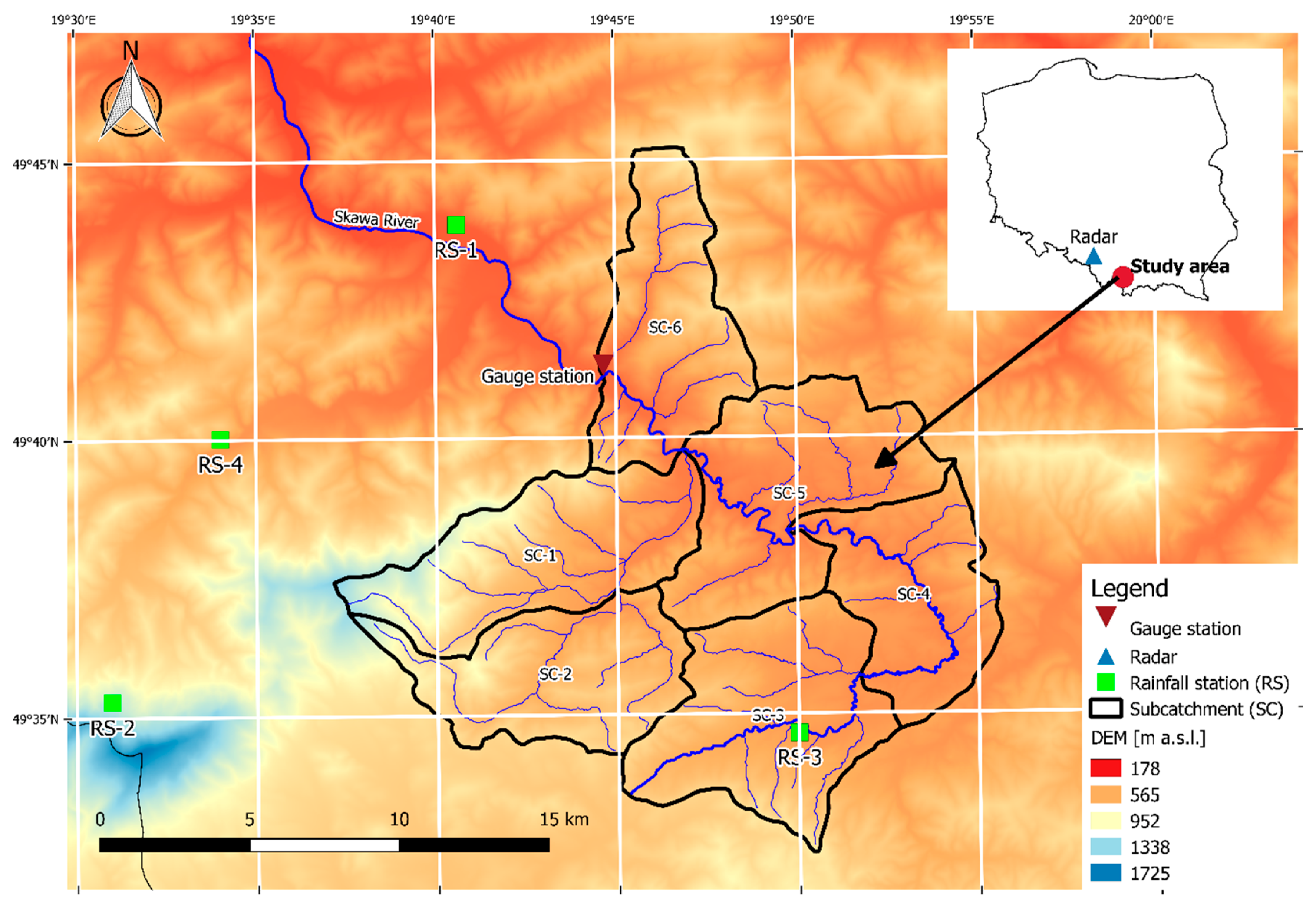
2.1. The Study Area

The Upper Skawa catchment is a small mountainous catchment in southern Poland. It is predominantly covered by non-irrigated arable lands and coniferous and mixed forests. The catchment, having total area of 240.4 km², can be sub-divided into six sub-catchments (Figure 1).

The annual rainfall of the sub-catchments ranges from 700 mm to 1200 mm. Besides that, the annual mean temperature up to 700 m a.s.l. varies from 4 °C to 6 °C, between 700–1100 m a.s.l. from 4 °C to 6 °C, and below 4 °C above 1100 m a.s.l. In the catchment area, there are four rain gauges, and one among them is located directly on-site. The discharge data are available at the river gauging station in Osielec. The closest meteorological radar is located in Ramża around 100 km north-west of research area.

2.2. Data Collection and Processing

Precipitation and discharge data used in this study were collected between 2014 and 2016. The beginning year of the analysis—2014, was chosen regarding the availability of the Global Precipitation Measurement (GPM) mission products. R software was used for statistical analysis and data processing.

2.2.1. Discharge Data

For calibration and validation of the HEC-HMS hydrological model, the discharge data from the gauging station in Osielec were applied. The runoff data (2014–2016) were provided by the Institute of Meteorology and Water Management–National Research Institute in Poland. During this period there were six flash flood events caused by excessive rainfall that were chosen for further analysis (

Table 1. Characteristics of the investigated flash flood events.

Event	Start	End	Maximum Discharge (m3/s)
Event 1	14 May 2014	23 May 2014	211.1
Event 2	3 October 2014	7 October 2014	22.8
Event 3	21 May 2015	30 May 2015	26.8
Event 4	14 May 2016	17 May 2016	19.9
Event 5	17 July 2016	19 July 2016	23.2
Event 6	3 October 2016	9 October 2016	35.2

).

Three aspects need to be highlighted when analyzing these flood events. Firstly, the Event 1 is characterized by significantly higher maximum discharge value than the other events. Secondly, the Event 1, Event 3, and Event 4 exhibit bimodal time distribution while the other events show unimodal distribution. Thirdly, Event 6 has the longest time of recession among the analyzed events. Therefore to provide a reliable and multi-aspect calibration of the model, Events 1, 2 and 6 were used in the calibration phase, whereas Events 3–5 served for the model validation. Additionally, it should be noted that the Event 1 has the maximum discharge 8 to 10 times of other events and precipitation rate plays a key role during this flood event.

2.2.2. Rain Gauges

The rain gauge data from the period 2014 to 2016 were provided to this research by the Institute of Meteorology and Water Management–National Research Institute in Poland. The 10-min time-step data were collected in four rain gauges located in the catchment area (

Table 2. Rainfall stations located nearby the study area.

Rainfall Station	Acronym	Longitude	Latitude
Maków Podhalański	RS-1	19°40′	49°43′
Markowe Szczawiny	RS-2	19°30′	49°35′
Spytkowice Górne	RS-3	19°50′	49°34′
Zawoja	RS-4	19°34′	49°40′

).

The rain gauges used in this study are part of the telemetric rain gauge network in Poland which consists of 491 gauges. The measurements are subject to automatically performed quality control concerning a range check using climatological values and analysis of the spatial and temporal consistency [34]. In this research the collected data were aggregated to 1-h intervals. Afterwards, the spatial distribution of precipitation was interpolated from the point data using the inverse distance weighting interpolation method (IDW). Like other interpolation algorithms it affects the spatial variability of the approximated rainfall distribution and therefore has an impact on discharge simulation. The IDW method is one of the most commonly used deterministic methods of spatial interpolation. However, recent studies (e.g., [35]) indicate that Radial Basis Function can estimate precipitation more precisely than IDW. As for geostatistical interpolation methods Ordinary Kriging and Co-Kriging are the most popular ones [36]. Some studies indicate that geostatistical approach of interpolation provide better results that deterministic one [37,38], but other studies report better performance of IDW than Kriging (e.g., [39]). Regardless of the method, the interpolation over mountainous areas is always challenging due to complex orography.

In this study, the IDW interpolation method was used for several reasons. Firstly, there is a built-in component in HEC-HMS which allows performing the IDW interpolation based on the rain gauge measurements provided by the user. Secondly, despite its limitations, the IDW method is often used to create spatial distribution of rainfall distribution (e.g., [34,40,41]). Thirdly, even if other interpolation methods may provide better spatial representation of precipitation field, in this study a semi-distributed hydrological model is used, and the interpolated values of rainfall rates are averaged over sub-catchments. Finally, the hyetographs, representing a mean value of precipitation in all the IDW interpolation cells that were within the boundaries of particular sub-catchment, were drawn for each of the sub-catchments.

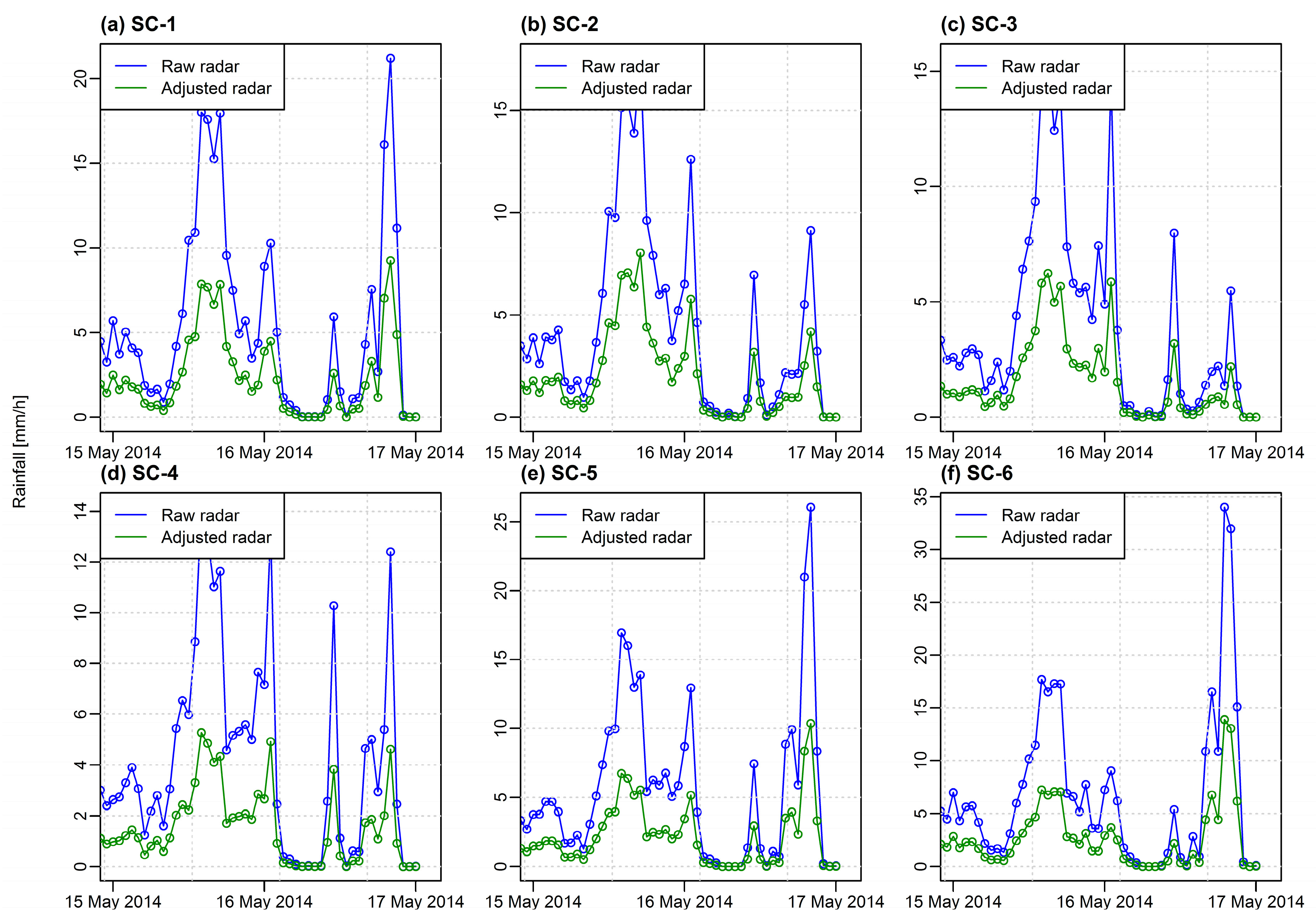
2.2.3. Radar Rainfall Estimates

The radar estimates were collected from the Ramża weather radar, which is a part of the Polish weather network POLRAD. The meteorological radar in Ramża is operating in a dual-polarization mode and frequency of 5600–5650 MHz (C-Band). These data (2014–2016) were also provided by the Institute of Meteorology and Water Management–National Research Institute in Poland. The product used in the study is called PAC (Precipitation Accumulation) and is retrieved using the formula which is expressed as follows [42]:

$$\mathrm{Z}=20\times {\mathrm{R}}^{0.13}$$

(1)

where: Z—radar reflectivity (mm⁶/m³), R—radar-derived rain amount (mm/h).

Before being released, the radar estimates are subject to the quality control regarding attenuation in heavy rain, anomalous propagation of the radar beam, beam blockage and hardware instability performed on raw data [34]. The PAC data were delivered in 10-min accumulations at spatial resolution of 1 × 1 km.

Radar-based rainfall estimates are associated with and effected by various sources of uncertainty. These are, among others, radar calibration, attenuation of radar signal, variability in the relationship between reflectivity (Z) and rainfall (R) and radar beam blockage. Calibration of the radar is associated with estimation of radar constant which is related to the radar technical components and thermal effects. The radar constant should be estimated within 1-db accuracy [43] otherwise the radar is considered as miscalibrated which may result in systematic over- or under-estimation of the rainfall estimates. Attenuation of radar antenna signal is the reduction of electromagnetic radiation power when passing through a medium of any density [14]—like clouds or rainfall. This problem mostly affects radars with short wavelengths (like C-band or X-band) [44], but can also be noticed for longer wavelengths (like S-band) [45]. The Z-R formula expresses the relation between reflectivity and rainfall rate for selected drop size distribution (DSD). For hydrological purposes, this relationship is frequently assumed to be constant in time and space even though it varies within rainfall intensity [46,47]. The complete or partial blockage of the radar beam caused by terrain or obstacles like buildings results in shielding of the radar beam. Over complex terrain, like mountainous environments, the beam shielding effect must be corrected before further application.

It is generally agreed that as the period of integration of radar estimates increases the mean difference between radar rainfall estimates and ground measurements performed by rain gauge (considered as ‘real’ precipitation) is decreasing [15,48,49]. Quantification of the radar rainfall estimates accuracy primarily depends on the applied adjustment method. It has been a subject of many studies, which demonstrated that without adjustment procedure, the errors in radars estimates are excessive [48]. For example Steiner et al. [50] used a high-quality gauge data and storm-based bias adjustment method and achieved root-mean-square errors of radar estimates of approximately 10% for rainfall accumulations greater than 30 mm. In other work the mean percentage difference of 15% close to the calibration site and up to 20% within a distance of 20 km was achieved by Harrold et al. [48] when the calibration process was performed using rain gauge measurements and the horizontal drift of the rain in the wind between the radar beam and the calibration site was allowed.

In the literature, one can find a considerable amount of papers dedicated to this subject e.g., [3,14,15,16]. Despite of all the challenges and limitations related to radar measurements of rainfall, the radar estimates are frequently used in the rainfall-runoff modeling (e.g., [8,9,19,51,52,53]).

2.2.4. Adjustment of Radar Rainfall Estimates Using Weighted Multiple Regression (WMR) Method

Before applying in hydrological modeling, the radar rainfall estimates should be adjusted (normalized) to reduce the measurement uncertainty. To mitigate the impact of orography and distance from the radar on measurement performance, the rainfall data were adjusted using weighted multiple regression (WMR) method, which, in this case, is expressed by multiple-linear relationship [18,54]:

$$\log \frac{\mathrm{R}}{\mathrm{G}}={\mathrm{a}}_1\times \mathrm{logDR}+{\mathrm{a}}_2\times \mathrm{MH}+{\mathrm{a}}_3\times \mathrm{HG}+{\mathrm{a}}_4,$$

(2)

where: R—radar-derived rain-amount (mm), G—time-accumulated rain gage amount (mm), DR—distance between the radar and the gauge (km), MH—minimum height that radar can target above the gage (m), HG—height of the gage (m a.s.l.), a₁–a₄—regression coefficients (-).

The WMR adjustment method aims to define the ratio between the time-accumulated precipitation measured by rain gauge and the corresponding radar estimate considering the orographic characteristics (parameters DR, MH, and HG in Equation (2)). With the growing distance between the radar and the gauge (DR) the altitude of the radar beam increases and the radar beam broadens. This to some extent is responsible for attenuation of radar signal which can result in under- or overestimation precipitation estimates at longer ranges [54]. The beam-shielding effect, which can be significant in the mountainous areas, is reflected by MH parameter indicating minimum height that must be reached by the radar beam to perform a proper measurement. The MH parameter corresponds to the measurement angle of radar. Therefore the lower is the MH value the better. Especially in the mountainous areas, the elevation effects have a significant influence on estimated precipitation as it may lead to the growth of precipitation related to orography. HG parameter in Equation (2) is to take this phenomenon under consideration. The Equation (2) doesn’t consider terrain slope which also has an impact on rainfall amount [55]. To minimize the uncertainty related to the mismatch of measurement in time 1-h accumulation of rainfall was used (instead of 10-min accumulations) for both rain gauge rainfall and radar estimates.

After all radar-gage data are substituted to the regression Equation (2) all coefficients a₁–a₄ can be estimated using, for instance, the least square method. Ultimately, the corrected radar estimate of precipitation at any location can be calculated from Equation (2) for any known value R, i.e., from radar-derived rain-amount. The corrected R-data serve as an input to the hydrological model of flow in the Upper Skawa catchment.

For the purpose of further analysis, the following assumptions are made:

• The spatial distribution of radar rainfall estimates corresponds to the rain gauge-based point measurements.
• Radar and rain gauge instruments perform the measurements at different heights, but the estimated rainfall from these instruments is assumed to be measured at the same level.
• The data analysis in each year is limited to the period from April to October to minimize the risk that radar would measure solid hydrometeors instead of liquid particles.
• Only simultaneous rainfall observations of rain gauge and radar are taken into further consideration; cases where only rain gauge or only radar registered rainfall were available are neglected.
• A semi-distributed hydrological model for each sub-catchment is assumed; mean value from all the radar estimates over the sub-catchment is assigned to its area. This mean value is accordingly adjusted and applied in the hydrological model.

2.2.5. IMERG GPM Satellite Rainfall Estimates

Since March 2014 the Global Precipitation Measurement (GPM) mission, led by the National Aeronautics and Space Administration (NASA) and the Japan Aerospace and Exploration Agency (JAXA), has provided quasi-global precipitation estimates. The GPM mission is a successor of the Tropical Rainfall Measuring Mission (TRMM) and aims at continuing satellite-based rainfall observations. GPM provides a wide variety of products, e.g., rainfall estimates that are data combined from active and passive instruments in the GPM constellation-Integrated Multisatellite Retrievals for GPM (IMERG).

In the study, IMERG version 4 (V04a) GPM-Level 3 Final Run products were used. They are derived from the IMERG algorithm, which is a post-real time research product released within a latency of 2.5 months. The IMERG algorithm intends to intercalibrate, merge, and interpolate different precipitation observations: satellite microwave precipitation estimates, satellite microwave-calibrated infrared precipitation estimates, monthly rain gauges measurements and other precipitation estimates [56]. These products include a gridded rainfall of a 0.1° × 0.1° spatial and 30 min temporal resolution. For the purpose of this study, we aggregated the data to 1-h accumulations. For each sub-catchment, a hyetograph was created, which represented a weighted mean value accounting the area of each sub-catchment covered by each grid.

IMERG data were provided by the NASA/Goddard Space Flight Center’s PMM and PSS teams from http://pmm.nasa.gov/data-access/.

2.2.6. Digital Elevation Model and Land-Cover

The Digital Elevation Model (DEM) of 100 m resolution was acquired from the Central Centre for Geodetic and Cartographic Documentation (currently Head Office of Geodesy and Cartography in Poland). Terrain complexity and DEM resolution have a significant impact on estimation of DEM hydrological derivatives (e.g., slopes) [57]. Using a low-resolution DEM in hydrological models might result in predicting lower peaks and higher baseflow compared to the use of high-resolution grid [58]. Therefore, using a coarser DEM resolution can generate worse results [57]. However, in this study, a semi-distributed hydrological model is applied and the slope information is used only in the Routing Model as a parameter of the river bed. More impact of DEM resolution on the flow model results should be expected when using fully distributed models. For adjustment of radar rainfall estimates (Section 3.1) DEM was upscaled to the resolution of radar precipitation field.

CORINE Land Cover Project CLC2012 v.18.5.1 was used as a source of land-cover information within the study area. A comprehensive description of land-cover delimitation for the study area can be found in Gilewski et al. [33].

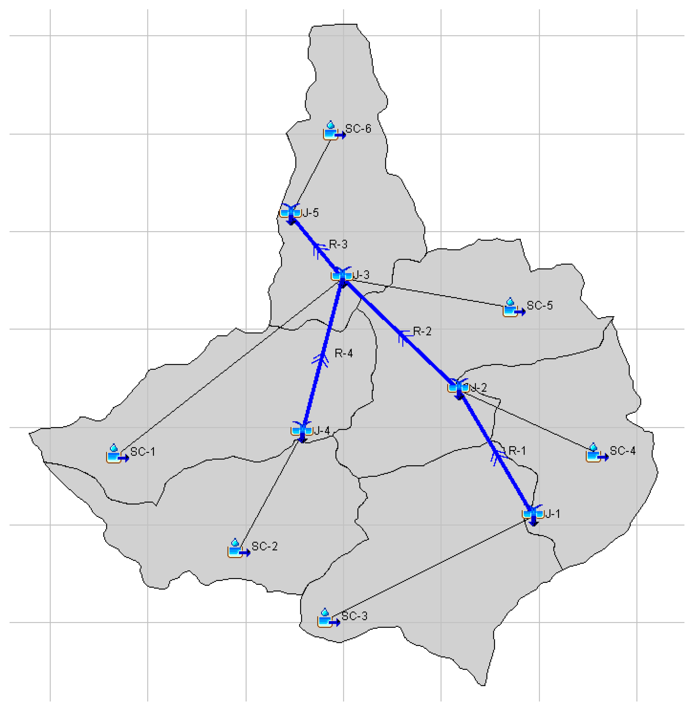
2.3. HEC-HMS Hydrological Model

To simulate basin runoff, HEC-HMS (Hydrologic Engineering Center-Hydrologic Modelling System) version 4.2.1. developed by the US Army Corps of Engineers was used. The HEC-HMS model is designed for both continuous and event-based modeling. In this study, methods which are primarily dedicated to event-based modeling were used.

2.3.1. Model Set-up

Two major input components of the HEC-HMS model are the catchment model and the meteorological model. The list of parameters and methods selected in the catchment modeling is shown in

Table 3. Selected methods for the Hydrologic Engineering Center-Hydrologic Modelling System (HEC-HMS).

Basin Model		Meteorological Model
Parameter Method	Selected Method	Parameter Method	Selected Method
Loss	SCS Curve Number	Precipitation	Inverse Distance (for rain gauges)
Transform	Snyder Unit Hydrograph		Specified Hyetograph (for radar and GPM)
Baseflow	Recession
Routing	Muskingum-Cunge

. A detailed description of the modeling concepts and equations behind for all the HEC-HMS sub-models and methods can be found in the technical reference manual by Feldman [59]. The initial values of parameters for the selected catchment modeling methods are provided in Section 3.3.1 along with the parameters’ values adjusted during the calibration process.

The Soil Conservation Service (SCS) Curve Number (CN) was the method used to estimate water losses. For incremental losses, the SCS-CN method uses the curve number methodology. The precipitation excess is estimated as a function of cumulative precipitation, soil cover, land-use, and antecedent moisture content. Land-use information was retrieved from CLC2012. For every sub-catchment, a weighted value of CN based on the land-use was calculated and fraction of impervious areas specified. Curve numbers were taken from standard tables [60]. The initial abstraction is considered as a precipitation depth before precipitation excess can occur. For each of the sub-catchment, the following parameters are to be specified: Initial Abstraction (mm), Curve Number (-) and Impervious Area (%).

A synthetic unit hydrograph (Snyder Unit Hydrograph), was chosen as a transform method to calculate the actual surface runoff. In this method, the unit hydrograph parameters are fitted for a sub-catchment using observed precipitation and discharge data. There are two parameters that were estimated for every sub-catchment: Standard Lag (h)—which is defined as the length of time between the centroid of precipitation mass and the peak flow of the resulting hydrograph; and Peaking Coefficient (-)—a measure of the steepness of the hydrograph resulting from a unit of precipitation.

Calculations of subsurface flow are performed by Recession Baseflow method which is primarily designed for event-based simulations. The method approximates the typical exponential shape of flow curve observed in the catchment when channel flow recedes after a flood event. For the sub-catchments the following parameters were specified: Initial Discharge (m³/s), Recession Constant (-)—rate at which the baseflow recedes between the flood events and Threshold Flow (m³/s)—specified flow value at which the baseflow is always reset when the receding limb of the hydrograph falls to that value.

For water routing in the river bed the Muskingum-Cunge Routing (MCRM) method was applied. It is based on the combination of the conservation of mass and the diffusion representation of the conservation of momentum.

In meteorological models considered in this research the Inverse Distance method was used to interpolate the precipitation data from rain gauges across the sub-catchments using the inverse-distance-squared weighting method. To specify time-series of hyetographs in sub-catchments the Specified Hyetograph method was used for radar and satellite data.

Figure 2 presents a schematic HEC-HMS hydrological model of the Upper Skawa Catchment. As a semi-distributed model was used, the catchment was sub-divided into six sub-catchments.

2.3.2. Calibration and Validation

Calibration and validation of the river flow model were carried out through comparing flow simulated by the model and the flow observed (at hourly time-steps) at the gauging station. Three out of six analyzed events were used for the calibration process. The peak-weighted RMSE metric was used as an objective function during the automatic calibration process for every event. Since precipitation intensity and its time distribution have a significant impact on the values of model parameters estimated during the calibration phase, the flow model was calibrated and validated separately for each of the three considered methods of measuring precipitation.

The selection of evaluation metrics should allow performing multi-aspect analysis of the models simulation results. Many diverse criteria are used to assess the performance efficiency of hydrological models [61]. Based on the literature [27,62,63] the following were used to compare the performance of the flow model in relation to the observed flows: NSE—broadly used for calibration and validation of hydrological models regarding discharge, r—primarily used for evaluation of the timing of simulated and observed time series, PBias—used to investigate the tendency of over- or underestimation of simulated flow, and rPFD—important criterion in terms of flood risk.

Nash-Sutcliffe efficiency coefficient (NSE) assess the predictive power of the model. It is defined as [64]:

$$\mathrm{NSE}=1-\frac{{\sum }_{\mathrm{i}=1}^{\mathrm{n}}{({\mathrm{Q}}_{\mathrm{obs}}-{\mathrm{Q}}_{\mathrm{sim}})}^2}{{\sum }_{\mathrm{i}=1}^{\mathrm{n}}{({\mathrm{Q}}_{\mathrm{obs}}-\overline{{\mathrm{Q}}_{\mathrm{obs}}})}^2}$$

(3)

where Q_sim and Q_obs are simulated and observed river flow, $\overline{{\mathrm{Q}}_{\mathrm{obs}}}$ is the mean of observed values and n is the number of observations. NSE values vary from −∞ to 1, where NSE = 1 means that the modeled discharge perfectly matches to the observed data, NSE = 0 indicates that the accuracy of the model prediction corresponds to the mean of the observation, while NSE < 0 means that the mean of observed flow is a better predictor than the model.

Pearson’s correlation coefficient [65] was used to measure the degree of linear association between simulated and observed flow. It is expressed as:

$$\mathrm{r}=1-\frac{{\sum }_{\mathrm{i}=1}^{\mathrm{n}}({\mathrm{Q}}_{\mathrm{sim}}-\overline{{\mathrm{Q}}_{\mathrm{sim}}})({\mathrm{Q}}_{\mathrm{obs}}-\overline{{\mathrm{Q}}_{\mathrm{obs}}})}{\sqrt{{\sum }_{\mathrm{i}=1}^{\mathrm{n}}{({\mathrm{Q}}_{\mathrm{sim}}-\overline{{\mathrm{Q}}_{\mathrm{sim}}})}^2}\sqrt{{\sum }_{\mathrm{i}=1}^{\mathrm{n}}{({\mathrm{Q}}_{\mathrm{obs}}-\overline{{\mathrm{Q}}_{\mathrm{obs}}})}^2}}$$

(4)

where Q_sim and Q_obs are simulated and observed river flow, $\overline{{\mathrm{Q}}_{\mathrm{sim}}}$ is the mean of simulated values $\overline{{\mathrm{Q}}_{\mathrm{obs}}}$ is the mean of observed values and n is the number of observations. Pearson’s correlation coefficient varies from −1 to 1.

To investigate the tendency of the simulated flow to over- or underestimate the observations the percent bias was used:

$$\mathrm{PBias}=\frac{{\sum }_{\mathrm{i}=1}^{\mathrm{n}}({\mathrm{Q}}_{\mathrm{sim}}-{\mathrm{Q}}_{\mathrm{obs}})}{{\sum }_{\mathrm{i}=1}^{\mathrm{n}}{\mathrm{Q}}_{\mathrm{obs}}}\times 100$$

(5)

where Q_sim and Q_obs are simulated and observed river flow. The ideal PBias value is equal to 0.

As the peak flow values are of particular interest regarding flood risk the relative peak flow difference metric was used:

$$\mathrm{rPFD}=\frac{{\mathrm{Q}}_{\mathrm{p},\mathrm{sim}}-{\mathrm{Q}}_{\mathrm{p},\mathrm{obs}}}{{\mathrm{Q}}_{\mathrm{p},\mathrm{obs}}}\times 100$$

(6)

where Q_p,sim and Q_p,obs are the peak values of simulated and observed river flow. The ideal value of rPFD is equal to 0. The accurate prediction of peak flow value is essential regarding flood risk forecasting across the river.

Table 4. Classification of performance for the selected performance metrics.

Performance Metrics	Value	Classification	Reference
Nash-Sutcliffe efficiency coefficient (NSE)	NSE ≤ 0.4	Unsatisfactory	[66]
	0.40–0.50	Acceptable
	0.50–0.65	Satisfactory
	0.65–0.75	Good
	0.75–1.00	Very Good
Pearson’s correlation coefficient (r)	r ≤ 0.4	Unsatisfactory	[29]
	0.40–0.60	Acceptable
	0.60–0.70	Satisfactory
	0.70–0.85	Good
	0.85–1.00	Very Good
Percent bias (PBias) Relative peak flow difference (rPFD)	>20%	Unacceptable	[63]
	≤20%	Acceptable

provides a classification of the performance of the metrics that were used for a model evaluation.

2.3.3. Simulation Time-Step Analysis

The initial time-step of the rainfall-runoff simulations was set up to 1-h interval. Generally, it can be observed that time aggregation of precipitation data reduces the bias between the observed and simulated data. With the increase in simulation time-step the probability of mismatch in time and space of rainfall measurements and rainfall estimates decreases. Therefore, one of the research goals was to check how the hydrological model performance changes for different time-step aggregations. All the simulated flows for validation period were computed using 2-, 3-, 4-, and 6-h time intervals. The performances of simulated hydrographs with aggregated time-steps were evaluated using the performance metrics described in Section 2.3.2.

3. Results and Discussion

3.1. Adjustment of Radar Rainfall Estimates

Table 5. Adjusted parameters for rain gauges and sub-catchments.

Parameter	Rain Gauges 1				Sub-Catchments 2
	GS-1	GS-2	GS-3	GS-4	SC-1	SC-2	SC-3	SC-4	SC-5	SC-6
DR (km)	82.8	84.9	101.7	80.8	91.6	94.5	100.8	102.4	96.9	90.4
HG (m a.s.l.)	367	1184	525	604	713.4	684.7	588.2	509.8	524.9	578.8
MH (m)	981.5	1434.1	1431.2	1011	1252.1	1482.4	1472.3	1384.8	1301.4	1067.1

¹ Point values for a rain gauge. ² Mean value for a sub-catchment.

shows the values of parameters DR, HG, and MH for locations of rain gauges, that were used to obtain the WMR coefficients, and the values of adjusted parameters for sub-catchments used for adjustment of radar rainfall estimates. It can be noticed that with the increasing distance from radar the minimum height that is targeted by radar is increasing. Moreover, complex topography in the mountainous region leads to an increase of the minimum height of radar beam due to its blockage by terrain elevation.

Using values of parameters for rain gauges from Table 5 along with rainfall measured at rain gauges and their corresponding radar rainfall estimates WMR coefficients of the relationship between R—radar-derived rain-amount (mm) and R’—time-accumulated adjusted radar-derived rain amount (mm) have been estimated:

$$\log \frac{\mathrm{R}}{{\mathrm{R}}^{\prime }}=4.48\times \mathrm{logDR}-{4.8}^{-4}\times \mathrm{MH}-{2.5}^{-5}\times \mathrm{HG}-\mathrm{7.34.}$$

(7)

To retrieve the adjusted radar rainfall estimate R^’ from Equation (7) values of radar-derived rain amount R and parameters DR, MH, and HG for sub-catchments from Table 5 were used.

Estimates of R^’ have been distributed over sub-catchments and compared to raw radar rainfall values—Figure 3.

After the adjustment process, the radar rainfall estimates values are significantly reduced compared to the raw data (around 40%). That may indicate that the raw radar rainfall estimates are overestimated. The same pattern was observed by Kawka et al. [52] when using a simple mean field bias radar data adjustment.

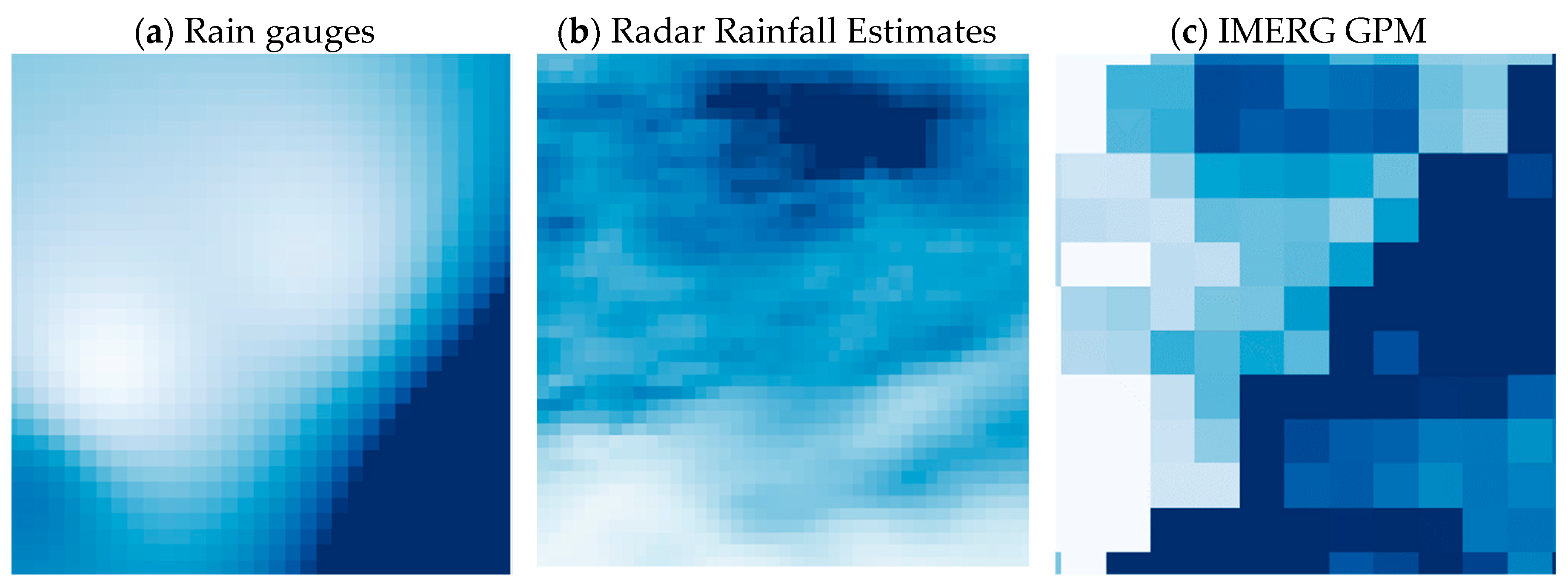
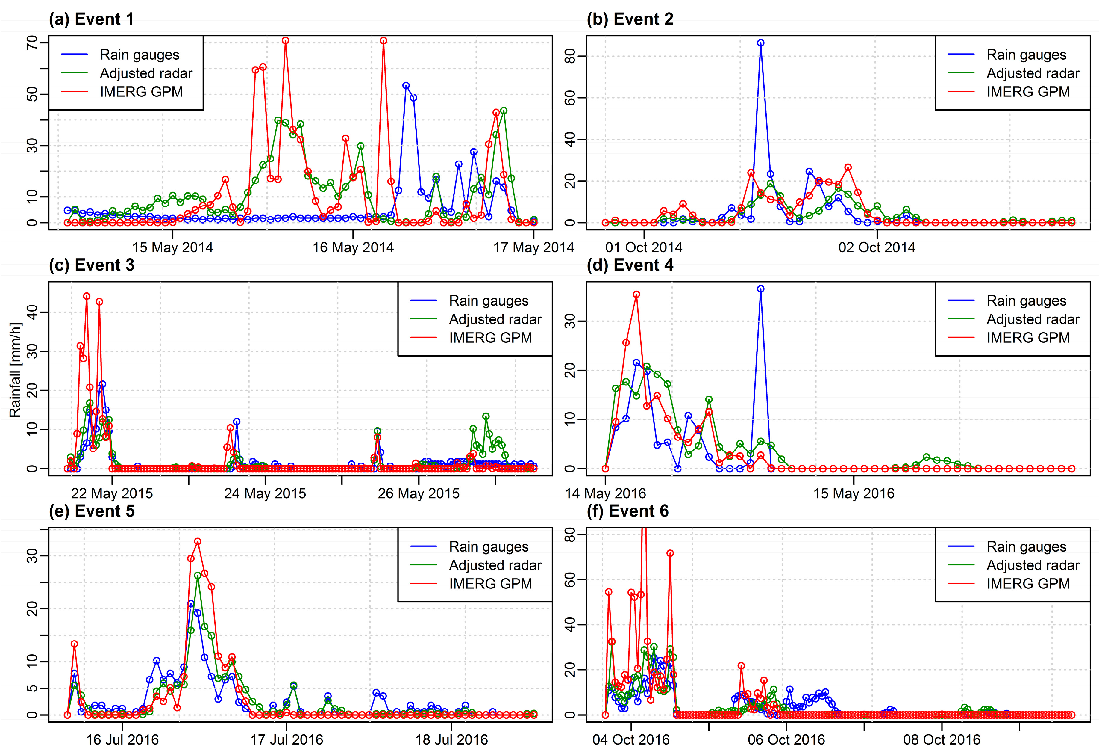
3.2. Intercomparison of Precipitation Products

As the result of measurement method used, three precipitation products applied in this research vary in terms of spatial and temporal resolution. Figure 4 shows spatial distribution of precipitation assessed by these products.

Temporal and spatial upscaling or downscaling of gridded precipitation data affect their accuracy and make them difficult to compare with each other. Interpolated precipitation field for sparsely gauged catchment might have a high degree of uncertainty and coarser spatiotemporal resolution than the satellite products. That may result in missing data while matching precipitation products of finer and coarser resolution [4]. To solve that problem Omranian et al. [67] suggested that application of precipitation product of higher spatiotemporal resolution may lead to better assessment of satellite products and successfully compared radar and IMERG GPM rainfall estimates by referring to the radar grid cell nearest to satellite product. Some of the satellite grids cells cover the areas outside the sub-catchments or are partially common for several sub-catchments. Therefore, it may happen that the rain being observed by the satellite is falling outside of the sub-catchments or partly into several ones. To take these aspects into account, for each sub-catchment, a hyetograph was created which represented a weighted mean accounting for the sub-catchment area covered by each grid. As for the rain gauge and radar precipitation data, distribution of rainfall rate for sub-catchments was created by taking a mean value from all the grid cells that could be found within sub-catchment boundaries.

Figure 5 presents the inter-comparison of precipitation products made for flood events 1–6. The information on total precipitation registered during the flood events is provided in

Table 6. Comparison of total precipitation for analyzed flood events.

Event	Total Precipitation Accumulation (mm)
	Rain Gauges	Raw Radar	Adjusted Radar	IMERG GPM
Event 1	397	1680	692	678
Event 2	212	437	179	223
Event 3	227	577	236	293
Event 4	129	452	184	149
Event 5	175	424	175	190
Event 6	448	1108	456	783

.

According to Table 6 during some of the flood events, the total accumulated precipitation calculated from different precipitation data sources is quite similar even temporal distribution of rainfall (Figure 5) during these events is different. The analyzed data sources of precipitation perform differently under extreme rainfall conditions. In most of the cases, the rain gauge rainfall seems to be underestimated and sensitive to registration of outliers. After adjustment, the radar rainfall estimates seem to have a smoother rainfall distribution that the other precipitation products and do not contain outlying values. It can be noticed that IMERG GPM rainfall estimates seem to be overestimated under the extreme rainfall conditions. The same pattern was observed for instance by Omranian et al. [67] when analyzing the performance of IMERG GPM rainfall data for Hurricane Harvey or by Prakash et al. [68] over India which is a monsoon dominated region.

Besides other reasons like model parameterization or temporal integration of water balance dynamics [69], the inaccuracy of the input data (in this case precipitation) is one of the main reasons for inaccuracy of the hydrological model. The occurrence of values that are probably outliers in the input precipitation may have a significant impact on calibration of the hydrological model. Taking into account the characteristics of the analyzed datasets of precipitation, results shown in Figure 5 and in Table 6 as well as topography of the study area one can expect that the adjusted radar rainfall estimates will perform the best and that the worst result will be obtained when using the rain gauge data. The performance of IMERG GPM data should be somewhere in between the other two sources of precipitation data.

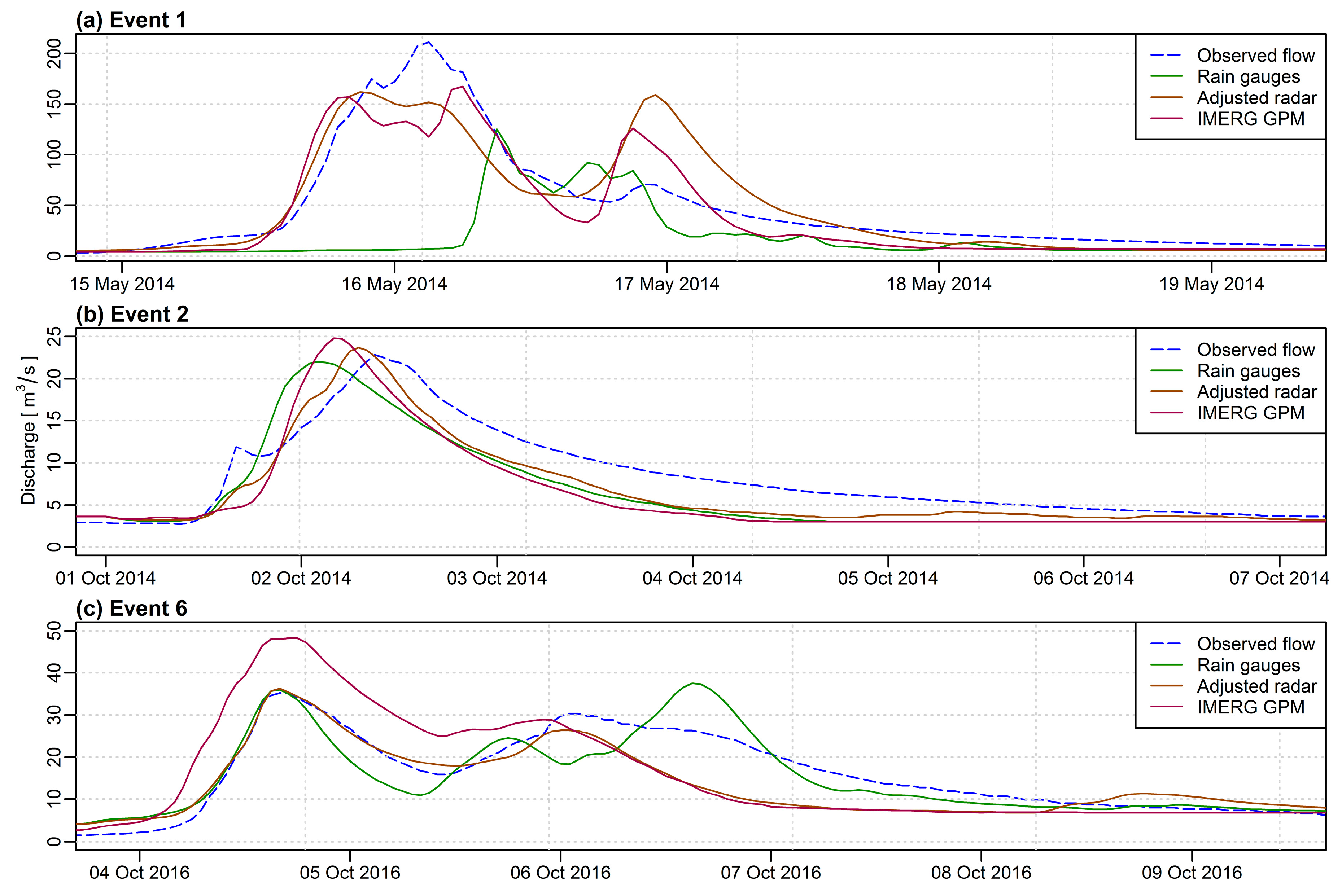
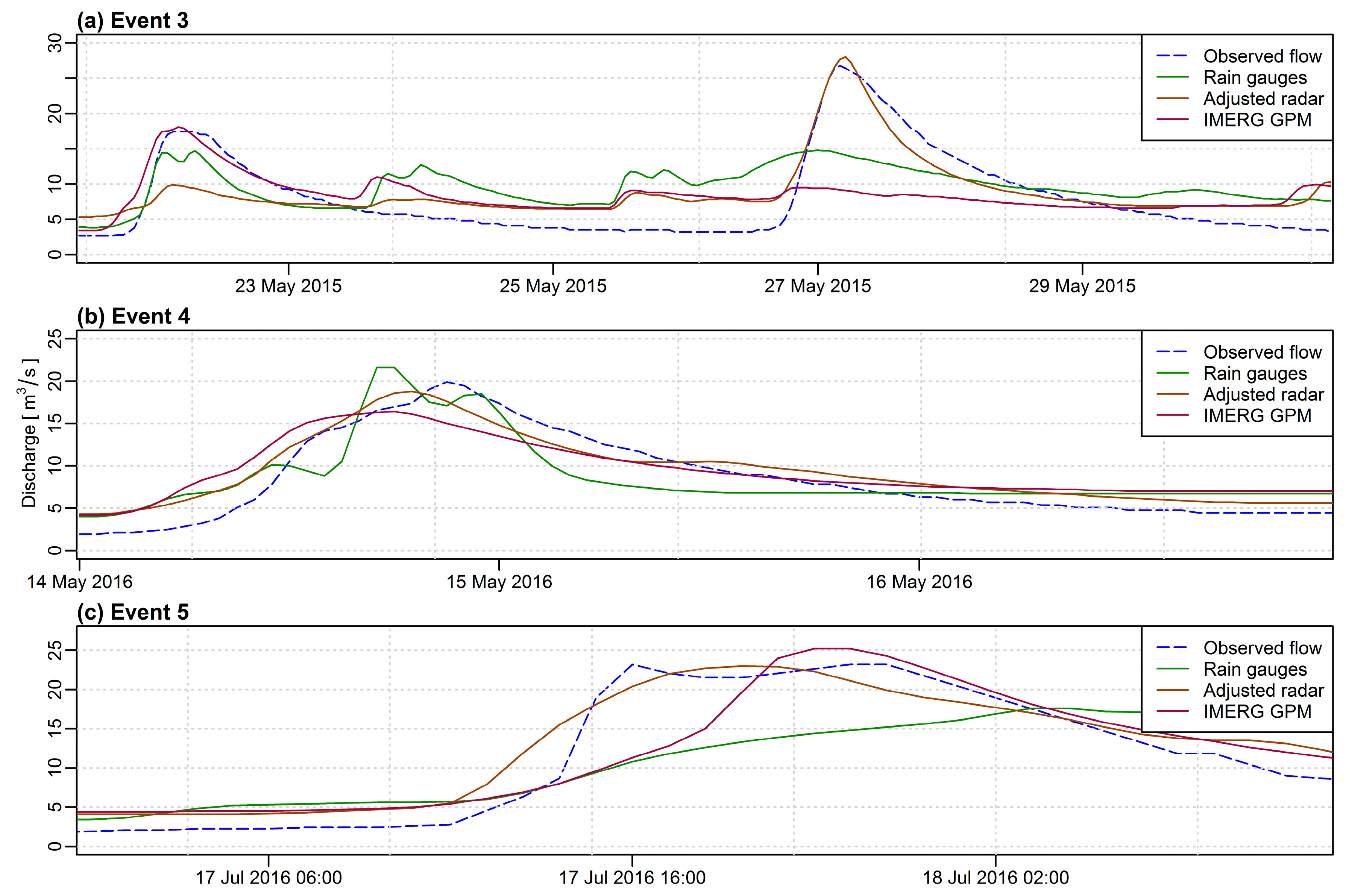
3.3. Simulation Results

3.3.1. Calibration and Validation of the Model

The results of evaluation criteria, described in Section 2.3.2, for three events used for calibration of the models are shown in

Table 7. The results of the evaluation criteria for calibration events.

Event	NSE			r			PBias (%)			rPFD
	Rain Gauges	Radar	IMERG	Rain Gauges	Radar	IMERG	Rain Gauges	Radar	IMERG	Rain Gauges	Radar	IMERG
Event 1	−0.46	0.79	0.81	0.17	0.89	0.90	−61.20	−0.60	−6.00	−40.6	−23.2	−20.7
Event 2	0.75	0.91	0.74	0.87	0.95	0.88	−2.30	−4.50	−4.50	−3.5	3.9	8.7
Event 6	0.78	0.66	0.20	0.89	0.84	0.76	−3.70	−13.50	0.50	6.5	3.1	36.9

. Figure 6 presents the comparison of observed and simulated hydrographs for the calibration events. The simulations of the outflow were performed at an hourly time steps.

Unsatisfactory performance of all performance metrics is observed for simulation of Event 1 while using rain gauges as precipitation data source. A good or very good performance of Nash–Sutcliffe efficiency coefficient (NSE), Pearson’s correlation coefficient (r) and Percent bias (PBias) can be observed for the rest of the analyzed cases. However, the outlook on the performance of Relative peak flow difference (rPFD) indicates that for all Event 1 simulation results are not acceptable. Therefore, even though the other metrics performed well for that event, the simulation results cannot be considered as acceptable. It’s worth noticing that there are cases (e.g., Event 6 simulated with IMERG-GPM precipitation data source) when some of the metrics (r and PBias) perform well while the other (NSE and rPFD) give unsatisfactory results. Therefore, the analysis of the selected simulations must be done regarding all performance metrics at the same time.

According to Figure 6, it can be noticed that the computed hydrographs agree well with the observed hydrographs particularly for the hydrological model run with adjusted radar precipitation estimates. The results of the hydrological model for Event 1, using adjusted radar and IMERG GPM precipitation estimates, show that an artificial second peak is produced. That may be a result of the chosen loss method (SCS Curve Number), which predicts an average trend of rainfall losses rather than the response of individual storm (particularly during the events of intense rainfall) [70]. All the hydrological models underestimated the peak flow values for Event 1. In the case of Event 2, all three hydrological models performed well, but the simulated peak value appeared earlier than the observed one. For Event 3 the hydrological model run with IMERG GPM precipitation as an input significantly overestimated the observed flow. Simulations for precipitation measured by rain gauges and adjusted radar estimates gave similar results regarding simulation of the first peak, whereas the second peak was respectively over- and underestimated.

Table 8. Calibrated model parameters for the Soil Conservation Service (SCS) Curve Number Loss Method.

Sub-Catchment	Initial Abstraction (MM)				Curve Number (-)
		Rain Gauges	Radar	IMERG		Rain Gauges	Radar	IMERG
	Initial	Optimized			Initial	Optimized
SC-1	25.23	19.42	26.57	21.83	43.02	48.63	70.68	54.27
SC-2	27.21	17.03	21.24	23.55	41.18	58.70	77.20	71.42
SC-3	17.77	13.73	15.23	15.38	51.73	86.64	87.11	75.52
SC-4	17.39	11.25	19.47	27.12	51.51	84.58	76.75	73.68
SC-5	17.01	16.48	12.92	21.83	52.82	63.07	81.71	73.49
SC-6	18.39	14.16	17.46	20.30	50.88	78.99	54.07	65.38

,

Table 9. Calibrated model parameters for Snyder Unit Hydrograph Transform Method.

Sub-Catchment	Standard Lag (HR)				Peaking Coefficient (-)
		Rain Gauges	Radar	IMERG		Rain Gauges	Radar	IMERG
	Initial	Optimized			Initial	Optimized
SC-1	1.74	1.54	2.75	2.07	0.4	0.49	0.36	0.19
SC-2	2.82	2.59	3.09	2.44	0.4	0.37	0.51	0.21
SC-3	2.82	2.61	2.96	2.86	0.4	0.40	0.26	0.20
SC-4	1.99	2.06	2.44	2.81	0.4	0.42	0.24	0.21
SC-5	1.77	2.31	2.16	2.58	0.4	0.37	0.32	0.22
SC-6	2.35	2.31	1.80	2.58	0.4	0.55	0.42	0.37

and

Table 10. Calibrated model parameters for Recession Base flow Method.

Sub-Catchment	Initial Discharge				Recession Constant					Threshold Discharge
		Rain Gauges	Radar	IMERG		Rain Gauges	Radar	IMERG		Rain Gauges	Radar	IMERG
	Initial	Optimized			Initial	Optimized			Initial	Optimized
SC-1	0.5	0.66	0.80	0.53	0.9	0.97	0.97	1.00	0.7	1.23	0.82	1.12
SC-2	0.5	0.59	0.67	0.66	0.9	1.00	1.00	1.00	0.7	1.23	0.70	1.00
SC-3	0.5	0.59	0.67	0.50	0.9	0.97	1.00	1.00	0.7	1.86	0.92	1.29
SC-4	0.5	0.51	0.59	0.66	0.9	0.97	1.00	0.97	0.7	1.00	0.94	0.82
SC-5	0.5	0.51	0.50	0.58	0.9	0.97	1.00	0.97	0.7	0.82	1.41	1.41
SC-6	0.5	0.93	0.80	0.58	0.9	0.97	0.97	1.00	0.7	0.93	1.00	1.12

provide calibrated model parameters values (which represent a mean from all three calibration events) for loss, transform and base flow methods assumed in the hydrological models and run with precipitation data from rain gauges, adjusted radar, and IMERG GPM.

The calibrated model parameters from Table 8, Table 9 and Table 10 were then used in the validation phase. The preliminary results indicated that the performance of the model is unsatisfactory when the model is run with constant values of the optimized parameters. Therefore, it was decided to implement a standard deviation interval of each parameter to the hydrological models and use it when validating the models.

Results of evaluation criteria, described in Section 2.3.2, for the events used for validation of the models are shown in

Table 11. The results of the evaluation criteria for validation events.

Event	NSE			r			PBias (%)			rPFD
	Rain Gauges	Radar	IMERG	Rain Gauges	Radar	IMERG	Rain Gauges	Radar	IMERG	Rain Gauges	Radar	IMERG
Event 3	0.28	0.69	0.21	0.61	0.85	0.47	18.10	9.50	3.50	−44.9	4.5	−32.5
Event 4	0.71	0.88	0.74	0.85	0.97	0.92	1.50	10.40	10.80	8.7	−5.4	−17.5
Event 5	−0.20	0.89	0.76	0.17	0.98	0.90	37.70	15.60	14.90	−15.1	−0.9	8.6

. Figure 7 contains the comparison of observed and simulated hydrographs for the validation events. Similarly, like in calibration stage, the simulations of the outflow were performed at an hourly time step.

As far as the validation stage is concerned the rain gauge-based simulations resulted in the most unsatisfactory performance of evaluation metrics. A good or very good performance is observed for all the validation events while using adjusted radar rainfall estimates. Except for Event 3, similar results are obtained for simulations with IMERG GPM data. However, the performance of rPFD criterion indicates that within the analyzed simulations the adjusted radar rainfall estimates perform the best. Alike the calibration events analysis, the overall evaluation of simulation must be done by considering all the performance metrics. For instance, if only performance PBias is taken into account it may result in the misleading conclusion that almost all simulations are acceptable.

The visual inspection of the simulated hydrographs—Figure 6, shows that they fit well to the observed ones for the simulations based on adjusted radar estimates and relatively well for Event 4 and Event 5 when IMERG GPM data are used. As to Event 3, in which river flow has a bimodal distribution, only adjusted radar estimates provide satisfactory results. The other simulations are not reproducing two peaks during one simulation. Most of the simulations present satisfactory results regarding the simulated peak flow value. However, in case of rain gauge and IMERG GPM simulations, there is a mismatch regarding the time of the peak occurrence.

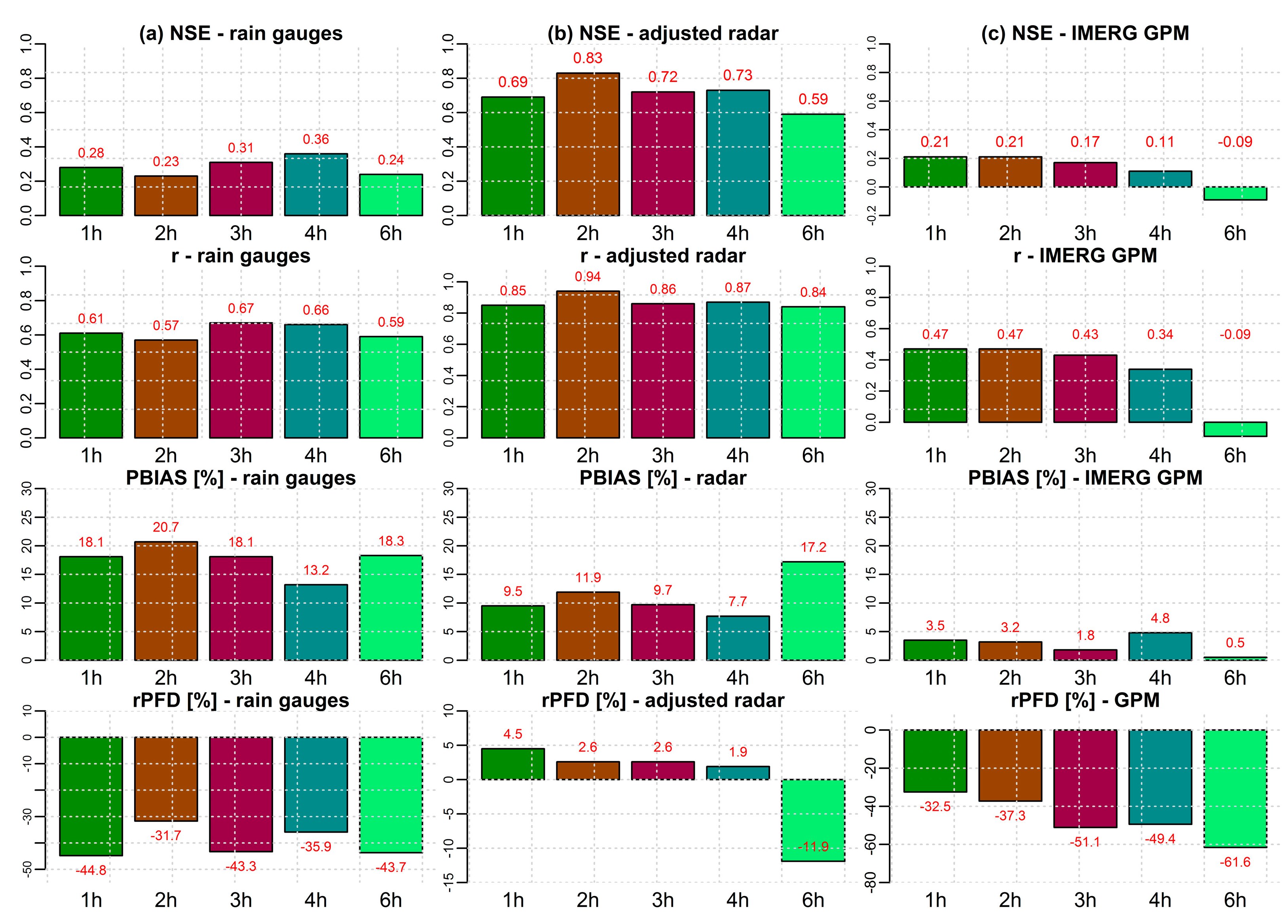
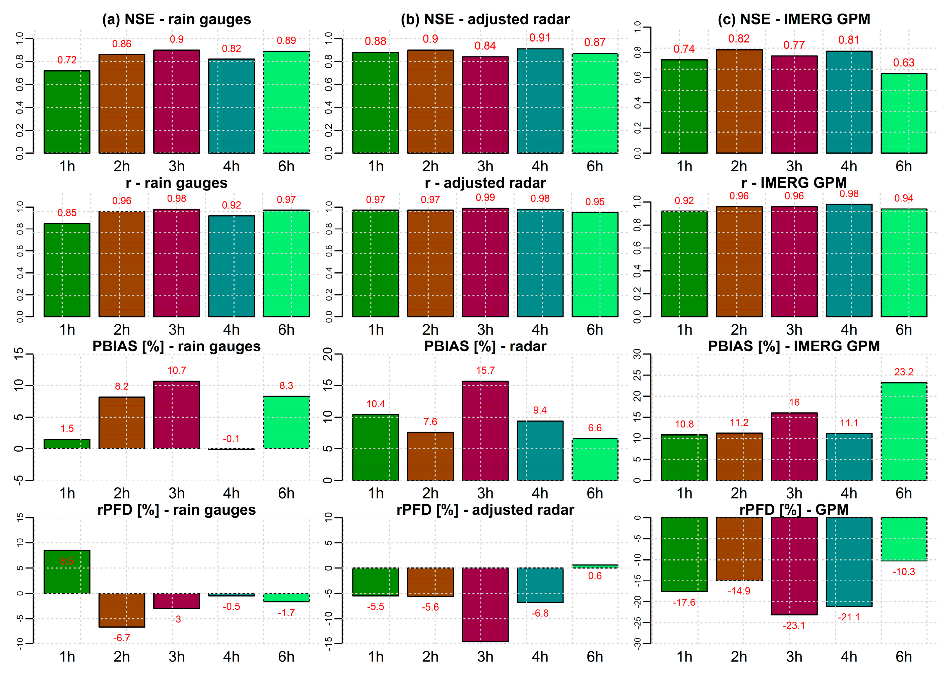
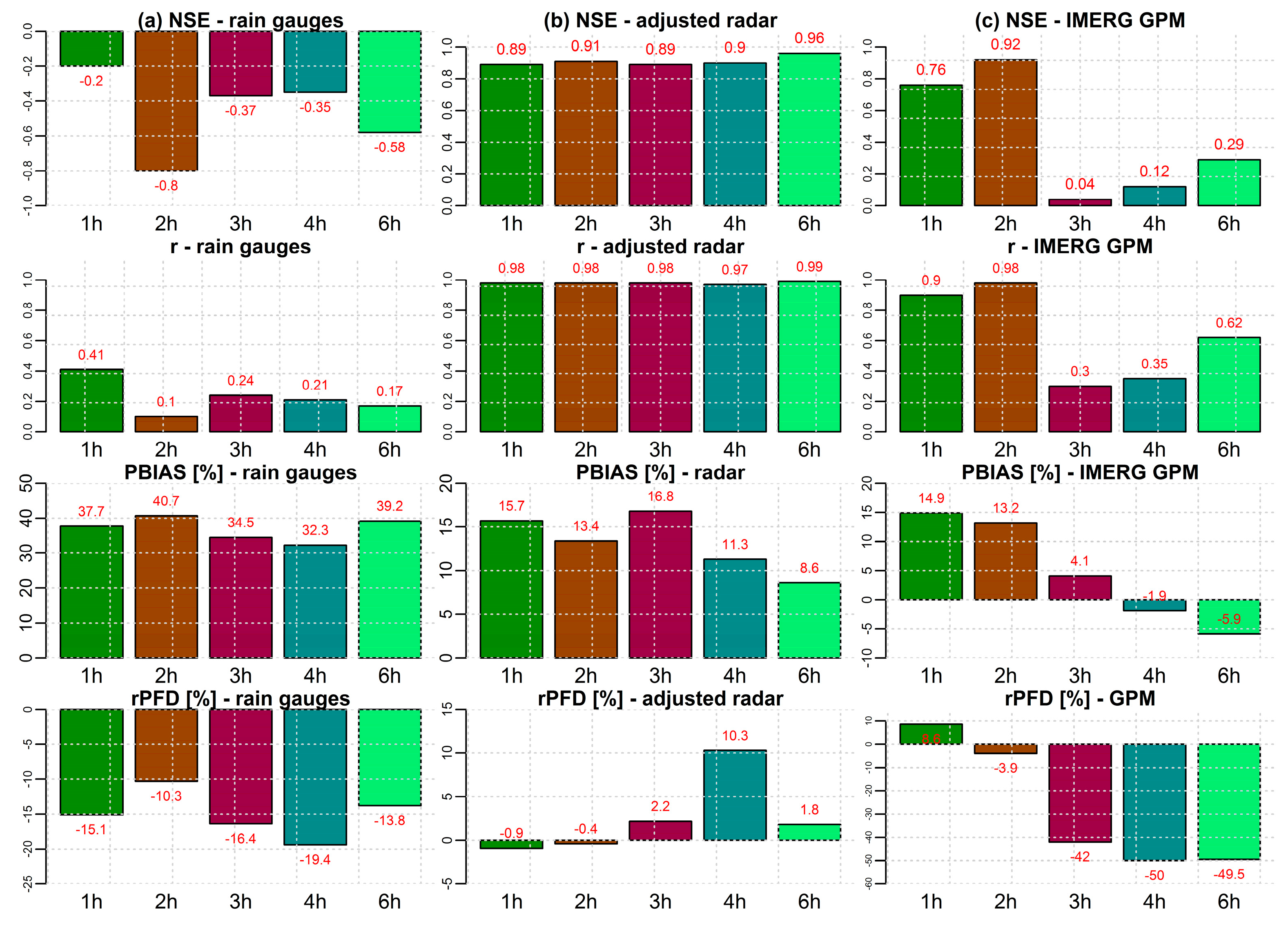
3.3.2. Simulation Time-Step Analysis

Figure 8, Figure 9 and Figure 10 show the values of performance metrics (NSE, r, PBias, rPFD) for validation events in reference to time-step intervals of hydrological model: 1-, 2-, 3-, 4-, and 6-h, respectively.

According to Figure 8, Figure 9 and Figure 10 for simulations using rain gauge precipitation the best results are obtained not for the initial time-step (1 h), but for the aggregated ones. Particularly, further aggregation in time longer than 2 h provide better results. That may indicate that the uncertainty of precipitation field created by interpolation from the rain gauge stations is quite significant. As for adjusted radar rainfall-based simulations the simulation results for 1- and 2-h time steps are similar, but generally slightly better for 2-h time step. Further aggregation in time in these cases does not provide better results. Simulations using IMERG GPM data give the best results for 1–2 h time step and longer time steps usually lead to a decrease of model performance. Therefore, it can be noticed that the optimal time-step of the simulation for the hydrological model using radar or IMERG GPM rainfall estimates is 1–2 h, whereas for rain gauges the time step should be extended. The worst results are obtained for aggregation in time up to 6-h which seem to be a too long time-step particularly for short event periods.

The observed deterioration of performance with increasing aggregation time-step is primarily related to the response time of the catchment. The average time to peak of the catchment is around 2.5 h (Table 9). Too much aggregated time-step (over the catchment response time) implicates the loss of information on the hydrological processes dynamics and lead to decrease of maximum discharge values. The aggregation of time-step has also impact on the estimation of model parameters which are time-dependent.

4. Conclusions

This paper presents a case study of rainfall-runoff modeling for a small mountainous catchment in southern Poland using three different precipitation data sets: rain gauge data, adjusted radar rainfall estimates and satellite rainfall (IMERG GPM). A semi-distributed HEC-HMS hydrological model was used for river flow simulation purposes. From the analysis of outcomes, the following conclusions can be drawn:

(1)

A good or very good model performance was obtained for most of the simulations during the calibration phase, but for the validation period, best results were obtained using the adjusted radar rainfall estimates and IMERG GPM data as precipitation data source.

(2)

Spatial and temporal distributions of rainfall estimated from different data sources vary significantly. As rainfall distribution in both time and space has a substantial impact on estimated values of model parameters a separate hydrological model should be applied for each source of the precipitation data.

(3)

Radar-estimated precipitation seems to be the most reliable source of information on the ‘real’ precipitation field. Precipitation interpolated from the rain gauge data seems to have a high degree of uncertainty, whereas IMERG GPM provides precipitation estimates of low spatial resolution.

(4)

Raw radar rainfall estimates seem to overestimate the observed rainfall significantly. Therefore, the radar data should be adjusted to minimize the bias between rain gauge measurement and radar estimation. When applied, the adjustment method for the radar rainfall estimates performed very well for event-based rainfall-runoff simulations in the mountainous area and can be easily adapted to other areas as it requires a relatively few data.

(5)

Short time of latency of IMERG GPM rainfall estimates makes it a valuable data source for near-real-time flood monitoring, but a rather sparse spatial resolution offsets this. Application of IMERG GPM rainfall estimates is challenging for small catchments as the satellite grids may cover the areas outside the sub-catchment or be partially common for several sub-catchment. If this is the case a weighting of rainfall should be done to account for the area of each sub-catchment covered by each grid.

(6)

Adequate choice of performance metrics is essential to evaluate the simulation results thoroughly. The evaluation criteria should allow judging the performance of the flow model regarding various flow characteristics (for the event-based modeling, these are predictive power of the model, timing of simulated and observed time series, tendency of over- or under-estimation of simulated flow, and accuracy in peak flow estimation). The applied evaluation metrics (Nash-Sutcliffe efficiency coefficient, Pearson’s correlation coefficient, percent bias, and relative peak flow difference) allowed to make a comprehensive assessment of simulation results regarding these characteristics.

(7)

Regardless of the values of the performance metrics, a visual analysis of the observed and simulated hydrographs should be performed. Sometimes the metrics can give satisfactory results even though the overall simulation results don’t fit the observed hydrograph.

(8)

Aggregation of simulation time-step up to 2 h improves the simulation results for radar- and satellite rainfall-based flow simulations. Further aggregation in time, up to 4 h, is valuable for simulations based on rain gauge precipitation data. The simulation results show that the time-step of simulations in a small catchment which have a short concentration time (like mountainous environments) should not exceed the response time of the catchment.

(9)

SCS Curve Number loss method applied in HEC-HMS is more adequate for simulations of flood events of unimodal distribution rather than of bimodal distribution. The method does not allow the regeneration of rainfall losses during the flood event and may lead to over- or underestimation of one of the flood event peaks.

References

1. Price, K.; Purucker, S.T.; Kraemer, S.R.; Babendreier, J.E.; Knightes, C.D. Comparison of radar and gauge precipitation data in watershed models across varying spatial and temporal scales. Hydrol. Process. 2014, 28, 3505–3520. [Google Scholar] [CrossRef]
2. Zubieta, R.; Getirana, A.; Espinoza, J.C.; Lavado, W. Impacts of satellite-based precipitation datasets on rainfall-runoff modeling of the Western Amazon basin of Peru and Ecuador. J. Hydrol. 2015, 528, 599–612. [Google Scholar] [CrossRef]
3. McKee, J.L.; Binns, A.D. A review of gauge–radar merging methods for quantitative precipitation estimation in hydrology. Can. Water Resour. J. 2016, 41, 186–203. [Google Scholar] [CrossRef]
4. Panthi, J.; Dahal, P.; Shrestha, M.; Aryal, S.; Krakauer, N.; Pradhanang, S.; Lakhankar, T.; Jha, A.; Sharma, M.; Karki, R. Spatial and temporal variability of rainfall in the Gandaki River Basin of Nepal Himalaya. Climate 2015, 3, 210–226. [Google Scholar] [CrossRef]
5. Barry, R.G. Changes in mountain climate and glacio-hydrological responses. Mt. Res. Dev. 1990, 10, 161–170. [Google Scholar] [CrossRef]
6. Gabella, M.; Speirs, P.; Hamann, U.; Germann, U.; Berne, A. Measurement of precipitation in the alps using dual-polarization C-Band ground-based radars, the GPM Spaceborne Ku-Band Radar, and rain gauges. Remote Sens. 2017, 9, 1147. [Google Scholar] [CrossRef]
7. Khalki, E.M.E.; Tramblay, Y.; Saidi, M.E.M.; Bouvier, C.; Hanich, L.; Benrhanem, M.; Alaouri, M. Comparison of modeling approaches for flood forecasting in the High Atlas Mountains of Morocco. Arab. J. Geosci. 2018, 11, 410. [Google Scholar] [CrossRef]
8. Sikorska, A.E.; Seibert, J. Value of different precipitation data for flood prediction in an alpine catchment: A Bayesian approach. J. Hydrol. 2018, 556, 961–971. [Google Scholar] [CrossRef]
9. Sikorska, A.E.; Seibert, J. Appropriate temporal resolution of precipitation data for discharge modelling in pre-alpine catchments. Hydrol. Sci. J. 2018, 63, 1–16. [Google Scholar] [CrossRef]
10. Looper, J.P.; Vieux, B.E. An assessment of distributed flash flood forecasting accuracy using radar and rain gauge input for a physics-based distributed hydrologic model. J. Hydrol. 2012, 412–413, 114–132. [Google Scholar] [CrossRef]
11. Tapiador, F.J.; Turk, F.J.; Petersen, W.; Hou, A.Y.; García-Ortega, E.; Machado, L.A.T.; Angelis, C.F.; Salio, P.; Kidd, C.; Huffman, G.J.; et al. Global precipitation measurement: Methods, datasets and applications. Atmos. Res. 2012, 104–105, 70–97. [Google Scholar] [CrossRef]
12. Mahmoud, M.T.; Al-Zahrani, M.A.; Sharif, H.O. Assessment of global precipitation measurement satellite products over Saudi Arabia. J. Hydrol. 2018, 559, 1–12. [Google Scholar] [CrossRef]
13. Guo, H.; Chen, S.; Bao, A.; Behrangi, A.; Hong, Y.; Ndayisaba, F.; Hu, J.; Stepanian, P.M. Early assessment of integrated multi-satellite retrievals for global precipitation measurement over China. Atmos. Res. 2016, 176–177, 121–133. [Google Scholar] [CrossRef]
14. Villarini, G.; Krajewski, W.F. Review of the different sources of uncertainty in single polarization radar-based estimates of rainfall. Surv. Geophys. 2010, 31, 107–129. [Google Scholar] [CrossRef]
15. Szturc, J. Niepewność w Radarowych Pomiarach Opadu z Punktu Widzenia Hydrologii; Instytut Meteorologii i Gospodarki Wodnej: Warszawa, Poland, 2010. [Google Scholar]
16. Berne, A.; Krajewski, W.F. Radar for hydrology: Unfulfilled promise or unrecognized potential? Adv. Water Resour. 2013, 51, 357–366. [Google Scholar] [CrossRef]
17. Sharifi, E.; Steinacker, R.; Saghafian, B. Assessment of GPM-IMERG and other precipitation products against gauge data under different topographic and climatic conditions in Iran: Preliminary results. Remote Sens. 2016, 8, 135. [Google Scholar] [CrossRef]
18. Gabella, M.; Amitai, E. Radar rainfall estimates in an alpine environment using different gage-adjustment techniques. Phys. Chem. Earth Part B Hydrol. Oceans Atmos. 2000, 25, 927–931. [Google Scholar] [CrossRef]
19. Keblouti, M.; Ouerdachi, L.; Berhail, S. The use of weather radar for rainfall-runoff modeling, case of Seybouse watershed (Algeria). Arab. J. Geosci. 2015, 8. [Google Scholar] [CrossRef]
20. Cecinati, F.; Rico-Ramirez, M.A.; Heuvelink, G.B.M.; Han, D. Representing radar rainfall uncertainty with ensembles based on a time-variant geostatistical error modelling approach. J. Hydrol. 2017, 548, 391–405. [Google Scholar] [CrossRef]
21. Sungmin, O.; Foelsche, U.; Kirchengast, G.; Fuchsberger, J.; Tan, J.; Petersen, W.A. Evaluation of GPM IMERG Early, Late, and Final rainfall estimates using WegenerNet gauge data in southeastern Austria. Hydrol. Earth Syst. Sci. 2017, 21, 6559–6572. [Google Scholar] [CrossRef] [Green Version]
22. Zubieta, R.; Geofísico, I.; Getirana, A. Hydrological modeling of the Peruvian–Ecuadorian Amazon Basin using GPM-IMERG satellite-based precipitation dataset. Hydrol. Earth Syst. Sci. 2017, 21, 3543–3555. [Google Scholar] [CrossRef] [Green Version]
23. Gosset, M.; Alcoba, M.; Roca, R.; Cloché, S.; Urbani, G. Evaluation of TAPEER daily estimates and other GPM era products against dense gauge networks in West Africa, analyzing ground reference uncertainty. Q. J. R. Meteorol. Soc. 2018. [Google Scholar] [CrossRef]
24. Mohsan, M.; Acierto, R.A.; Kawasaki, A.; Zin, W.W. Preliminary assessment of GPM satellite rainfall over Myanmar. J. Disaster Res. 2018, 13, 22–30. [Google Scholar] [CrossRef]
25. Knebl, M.R.; Yang, Z.L.; Hutchison, K.; Maidment, D.R. Regional scale flood modeling using NEXRAD rainfall, GIS, and HEC-HMS/RAS: A case study for the San Antonio River Basin Summer 2002 storm event. J. Environ. Manag. 2005, 75, 325–336. [Google Scholar] [CrossRef] [PubMed]
26. Halwatura, D.; Najim, M.M.M. Application of the HEC-HMS model for runoff simulation in a tropical catchment. Environ. Model. Softw. 2013, 46, 155–162. [Google Scholar] [CrossRef]
27. Bhuiyan, H.A.K.M.; McNairn, H.; Powers, J.; Merzouki, A. Application of HEC-HMS in a cold region watershed and use of RADARSAT-2 soil moisture in initializing the model. Hydrology 2017, 4, 9. [Google Scholar] [CrossRef]
28. Ren, J.; Zheng, X.; Chen, P.; Zhao, X.; Chen, Y.; Shen, Y. An investigation into sub-basin rainfall losses in different underlying surface conditions using HEC-HMS: A case study of a loess hilly region in Gedong basin in the western Shanxi Province of China. Water 2017, 9, 870. [Google Scholar] [CrossRef]
29. Rauf, A.; Ghumman, A.R. Impact assessment of rainfall-runoff simulations on the flow duration curve of the Upper Indus River—A comparison of data-driven and hydrologic models. Water 2018, 10, 876. [Google Scholar] [CrossRef]
30. Chen, Y.; Xu, Y.; Yin, Y. Impacts of land use change scenarios on storm-runoff generation in Xitiaoxi basin, China. Quat. Int. 2009, 208, 121–128. [Google Scholar] [CrossRef]
31. Ali, M.; Khan, S.J.; Aslam, I.; Khan, Z. Simulation of the impacts of land-use change on surface runoff of Lai Nullah Basin in Islamabad, Pakistan. Landsc. Urban Plan. 2011, 102, 271–279. [Google Scholar] [CrossRef]
32. Zope, P.E.; Eldho, T.I.; Jothiprakash, V. Impacts of land use-land cover change and urbanization on flooding: A case study of Oshiwara River Basin in Mumbai, India. Catena 2016, 145, 142–154. [Google Scholar] [CrossRef]
33. Gilewski, P.; Węglarz, A. Impact of land-cover change related urbanization on surface runoff estimation. EDP Sci. 2018, 196. [Google Scholar] [CrossRef]
34. Szturc, J.; Jurczyk, A.; Ośródka, K.; Wyszogrodzki, A.; Giszterowicz, M. Precipitation estimation and nowcasting at IMGW-PIB (SEiNO system). Meteorol. Hydrol. Water Manag. Res. Oper. Appl. 2018, 6. [Google Scholar] [CrossRef]
35. Luo, X.; Xu, Y.; Xu, J. Application of radial basis function network for spatial precipitation interpolation. In Proceedings of the 18th International Conference on Geoinformatics, Beijing, China, 18–20 June 2010; pp. 1–5. [Google Scholar]
36. Mair, A.; Fares, A. Comparison of rainfall interpolation methods in a mountainous region of a tropical island. J. Hydrol. Eng. 2011, 16, 371–383. [Google Scholar] [CrossRef]
37. Drogue, G.; Humbert, J.; Deraisme, J.; Mahr, N.; Freslon, N. A statistical-topographic model using an omnidirectional parameterization of the relief for mapping orographic rainfall. Int. J. Climatol. 2002, 22, 599–613. [Google Scholar] [CrossRef] [Green Version]
38. Buytaert, W.; Celleri, R.; Willems, P.; Bièvre, B.D.; Wyseure, G. Spatial and temporal rainfall variability in mountainous areas: A case study from the south Ecuadorian Andes. J. Hydrol. 2006, 329, 413–421. [Google Scholar] [CrossRef] [Green Version]
39. Kong, Y.F.; Tong, W.W. Spatial exploration and interpolation of the surface precipitation data. Geogr. Res. 2008, 27, 1097–1108. [Google Scholar] [CrossRef]
40. Kurtzman, D.; Navon, S.; Morin, E. Improving interpolation of daily precipitation for hydrologic modelling: Spatial patterns of preferred interpolators. Hydrol. Process. 2009, 23, 3281–3291. [Google Scholar] [CrossRef]
41. Chen, F.-W.; Liu, C.-W. Estimation of the spatial rainfall distribution using inverse distance weighting (IDW) in the middle of Taiwan. Paddy Water Environ. 2012, 10, 209–222. [Google Scholar] [CrossRef]
42. Tuszyńska, I. Charakterystyka Produktów Radarowych; Instytut Meteorologii i Gospodarki Wodnej: Warszawa, Poland, 2011. [Google Scholar]
43. Atlas, D. Radar calibration: Some simple approaches. Bull. Am. Meteorol. Soc. 2002, 83, 1313–1316. [Google Scholar] [CrossRef]
44. Uijlenhoet, R.; Berne, A. Stochastic simulation experiment to assess radar rainfall retrieval uncertainties associated with attenuation and its correction. Hydrol. Earth Syst. Sci. 2008, 12, 587–601. [Google Scholar] [CrossRef] [Green Version]
45. Ryzhkov, A.; Zrnic, D.S. Precipitation and attenuation measurements at a 10-cm Wavelength. J. Appl. Meteorol. 1995, 34, 2121–2134. [Google Scholar] [CrossRef]
46. Tokay, A.; Kruger, A.; Krajewski, W.F. Comparison of drop size distribution measurements by impact and optical disdrometers. J. Appl. Meteorol. 2001, 40, 2083–2097. [Google Scholar] [CrossRef]
47. Smith, J.A.; Hui, E.; Steiner, M.; Baeck, M.L.; Krajewski, W.F.; Ntelekos, A.A. Variability of rainfall rate and raindrop size distributions in heavy rain. Water Resour. Res. 2009, 45. [Google Scholar] [CrossRef] [Green Version]
48. Harrold, T.W.; English, E.J.; Nicholass, C.A. The accuracy of radar-derived rainfall measurements in hilly terrain. Q. J. R. Meteorol. Soc. 1974, 100, 331–350. [Google Scholar] [CrossRef]
49. Seo, D.-J.; Breidenbach, J.P. Real-time correction of spatially nonuniform bias in radar rainfall data using rain gauge measurements. J. Hydrometeorol. 2002, 3, 93–111. [Google Scholar] [CrossRef]
50. Steiner, M.; Smith, J.A.; Burges, S.J.; Alonso, C.V.; Darden, R.W. Effect of bias adjustment and rain gauge data quality control on radar rainfall estimation. Water Resour. Res. 1999, 35, 2487–2503. [Google Scholar] [CrossRef] [Green Version]
51. Szturc, J.; Ośródka, K.; Jurczyk, A.; Jelonek, L. Concept of dealing with uncertainty in radar-based data for hydrological purpose. Nat. Hazards Earth Syst. Sci. 2008, 8, 267–279. [Google Scholar] [CrossRef] [Green Version]
52. Kawka, M.; Przyborowski, Ł.; Nawalany, M. Możliwości wykorzystania produktów radarowych w celu poprawy jakości prognozy modelu opad-odpływ. In Monografie Komitetu Inżynierii Środowiska Polskiej Akademii Nauk; Komitet Inżynierii Środowiska PAN: Warszawa, Poland, 2014; ISBN 978-83-63714-18-5. [Google Scholar]
53. Niemi, T.J.; Warsta, L.; Taka, M.; Hickman, B.; Pulkkinen, S.; Krebs, G.; Moisseev, D.N.; Koivusalo, H.; Kokkonen, T. Applicability of open rainfall data to event-scale urban rainfall-runoff modelling. J. Hydrol. 2017, 547, 143–155. [Google Scholar] [CrossRef]
54. Gabella, M.; Joss, J.; Perona, G.; Galli, G. Accuracy of rainfall estimates by two radars in the same Alpine environment using gage adjustment. J. Geophys. Res. 2001, 106, 5139–5150. [Google Scholar] [CrossRef] [Green Version]
55. Blocken, B.; Poesen, J.; Carmeliet, J. Impact of wind on the spatial distribution of rain over micro-scale topography: Numerical modelling and experimental verification. Hydrol. Process. 2006, 20, 345–368. [Google Scholar] [CrossRef]
56. Huffman, G.J.; Bolvin, D.T.; Braithwaite, D.; Hsu, K.; Joyce, R.; Kidd, C.; Nelkin, E.J.; Sorooshian, S.; Tan, T.; Xie, P. NASA Global Precipitation Measurement (GPM) Integrated Multi-satellitE Retrievals for GPM (IMERG)—Algorithm Theoretical Basis Document (ATBD) Version 5.2; National Aeronautics and Space Administration: Washington, DC, USA, 2018. [Google Scholar]
57. Tang, G.; Hui, Y.; Strobl, J.; Liu, W. The impact of resolution on the accuracy of hydrologic data derived from DEMs. J. Geogr. Sci. 2001, 11, 393–401. [Google Scholar] [CrossRef]
58. Kenward, T.; Lettenmaier, D.P.; Wood, E.F.; Fielding, E. Effects of digital elevation model accuracy on hydrologic predictions. Remote Sens. Environ. 2000, 74, 432–444. [Google Scholar] [CrossRef]
59. US Army Corps of Engineers (USACE). Hydrologic Modeling System HEC-HMS: Technical Reference Manual; Hydrologic Engineering Center: Davis, CA, USA, 2000. [Google Scholar]
60. Kibler, D.F. Urban Stormwater Hydrology; American Geophysical Union: Washington, DC, USA, 1982. [Google Scholar]
61. Krause, P.; Boyle, D.P.; Bäse, F. Comparison of different efficiency criteria for hydrological model assessment. Adv. Geosci. 2005, 5, 89–97. [Google Scholar] [CrossRef]
62. Zelelew, D.; Melesse, A. Applicability of a spatially semi-distributed hydrological model for watershed scale runoff estimation in Northwest Ethiopia. Water 2018, 10, 923. [Google Scholar] [CrossRef]
63. Fang, G.; Yuan, Y.; Gao, Y.; Huang, X.; Guo, Y. Assessing the effects of urbanization on flood events with urban agglomeration polders type of flood control pattern using the HEC-HMS model in the Qinhuai River Basin, China. Water 2018, 10, 1003. [Google Scholar] [CrossRef]
64. Nash, J.E.; Sutcliffe, J.V. River flow forecasting through conceptual models part I—A discussion of principles. J. Hydrol. 1970, 10, 282–290. [Google Scholar] [CrossRef]
65. Pearson, K. Mathematical contributions to the theory of evolution—On a form of spurious correlation which may arise when indices are used in the measurement of organs. Proc. R. Soc. Lond. 1896, 60, 489–498. [Google Scholar] [CrossRef]
66. Moriasi, D.N.; Arnold, J.G.; Van Liew, M.W.; Bingner, R.L.; Harmel, D.; Veith, T.L. Model evaluation guidelines for systematic quantification of accuracy in watershed simulations. Trans. ASAB 2007, 50, 885–900. [Google Scholar] [CrossRef]
67. Omranian, E.; Sharif, H.O.; Tavakoly, A.A. How well can Global Precipitation Measurement (GPM) capture hurricanes? Case study: Hurricane harvey. Remote Sens. 2018, 10, 1150. [Google Scholar] [CrossRef]
68. Prakash, S.; Mitra, A.K.; AghaKouchak, A.; Liu, Z.; Norouzi, H.; Pai, D.S. A preliminary assessment of GPM-based multi-satellite precipitation estimates over a monsoon dominated region. J. Hydrol. 2018, 556, 865–876. [Google Scholar] [CrossRef]
69. Schoups, G.; Vrugt, J.A.; Fenicia, F.; van de Giesen, N.C. Corruption of accuracy and efficiency of Markov chain Monte Carlo simulation by inaccurate numerical implementation of conceptual hydrologic models. Water Resour. Res. 2010, 46. [Google Scholar] [CrossRef] [Green Version]
70. Mishra, S.K.; Suresh Babu, P.; Singh, V.P. SCS-CN method revisited. In Advances in Hydraulics and Hydrology; Water Resources Publications: Littleton, CO, USA, 2007. [Google Scholar]
Figure 1. Location of the study area—the Upper Skawa River catchment, in reference to digital elevation model (DEM) and the map of Poland.
Water 10 01665 g001
Figure 2. The schematic model of the Upper Skawa Catchment created in HEC-HMS. The names of sub-catchments, junctions and reaches are abbreviated with SC, J, and R, respectively.
Water 10 01665 g002
Figure 3. Comparison of raw and adjusted radar rainfall estimates for Event 1 (adapted to the period of significant precipitation): (a) SC-1; (b) SC-2; (c) SC-3; (d) SC-4; (e) SC-5; (f) SC-6.
Water 10 01665 g003
Figure 4. Comparison of gridded precipitation data: (a) Rain gauges—interpolated point data (1 × 1 km); (b) Radar—radar rainfall estimates (1 × 1 km); and (c) IMERG GPM—satellite precipitation (11 × 11 km).
Water 10 01665 g004
Figure 5. Comparison of the temporal distribution of 1-h rainfall accumulation (for the entire catchment) for rain gauges, adjusted radar, and IMERG GPM data during the analyzed events 1–6 (af).
Water 10 01665 g005
Figure 6. Comparison of simulated and observed hydrographs for the calibration events (a) Event 1: 14–23 May 2014, (b) Event 2: 3–7 October 2014, (c) Event 6: 3–9 October 2016.
Water 10 01665 g006
Figure 7. Comparison of simulated and observed hydrographs for the validation events (a) Event 3: 21–30 May 2015, (b) Event 4: 14–17 May 2016, (c) Event 5: 17–19 July 2016.
Water 10 01665 g007
Figure 8. Comparison of the evaluation metrics performance (in columns) for Event 3 for aggregated time-steps simulations based on (a) rain gauge precipitation, (b) adjusted radar rainfall estimates, (c) IMERG GPM satellite rainfall estimates.
Water 10 01665 g008
Figure 9. Comparison of the evaluation metrics performance (in columns) for Event 4 for aggregated time-steps simulations based on (a) rain gauge precipitation, (b) adjusted radar rainfall estimates, (c) IMERG GPM satellite rainfall estimates.
Water 10 01665 g009
Figure 10. Comparison of the evaluation metrics performance (in columns) for Event 5 for aggregated time-steps simulations based on (a) rain gauge precipitation, (b) adjusted radar rainfall estimates, (c) IMERG GPM satellite rainfall estimates.
Water 10 01665 g010