Object-Based Convolutional Neural Networks for Cloud and Snow Detection in High-Resolution Multispectral Imagers


1
College of Architectural Engineering, Heilongjiang University of Science and Technology, Harbin 150022, China
2
College of Landscape Architecture, Northeast Forestry University, Harbin 150040, China
3
College of Agricultural and Life Sciences, University of Wisconsin, Madison, WI 53706, USA
4
State Key Laboratory of Information Engineering in Surveying, Mapping and Remote Sensing, Wuhan University, Wuhan 430079, China
5
Chinese Academy of Surveying and Mapping, Beijing 100830, China
6
College of Wildlife Resources, Northeast Forestry University, Harbin 150040, China
*
Authors to whom correspondence should be addressed.
†
These authors contributed equally to this work.
Water 2018, 10(11), 1666; https://doi.org/10.3390/w10111666
Submission received: 15 October 2018
/
Revised: 9 November 2018
/
Accepted: 12 November 2018
/
Published: 15 November 2018
(This article belongs to the Special Issue Satellite Remote Sensing and Analyses of Climate Variability)
Abstract
:Cloud and snow detection is one of the most significant tasks for remote sensing image processing. However, it is a challenging task to distinguish between clouds and snow in high-resolution multispectral images due to their similar spectral distributions. The shortwave infrared band (SWIR, e.g., Sentinel-2A 1.55–1.75 µm band) is widely applied to the detection of snow and clouds. However, high-resolution multispectral images have a lack of SWIR, and such traditional methods are no longer practical. To solve this problem, a novel convolutional neural network (CNN) to classify cloud and snow on an object level is proposed in this paper. Specifically, a novel CNN structure capable of learning cloud and snow multiscale semantic features from high-resolution multispectral imagery is presented. In order to solve the shortcoming of “salt-and-pepper” in pixel level predictions, we extend a simple linear iterative clustering algorithm for segmenting high-resolution multispectral images and generating superpixels. Results demonstrated that the new proposed method can with better precision separate the cloud and snow in the high-resolution image, and results are more accurate and robust compared to the other methods.
1. Introduction
High-resolution images are widely used in land cover monitoring, target detection and geographic mapping [1]. Cloud and snow significantly influence the spectral bands of high-resolution optical images [2].
Accurate detection of clouds and snow for remote sensing images is a key task for many remote sensing applications [3]. The presence of cloud and snow can cause serious problems for many remote sensing applications such as target recognizing segmentation, atmosphere correction, and more [4]. Therefore, the precise detection of clouds and snow in optical satellite image applications is quite challenging work.
Previous methods for cloud and snow detection have been developed based on spectral analysis [5]. In the existing methods, the shortwave infrared band (SWIR, e.g., Sentinel-2A 1.55–1.75 µm band) is widely applied to the detection of snow and clouds [6]. The main reason is that the reflectance of snow is commonly lower than clouds at SWIR wavelengths [7]. The Normalized Difference Snow Index (NDSI) [8], a combination of visible (green band) and SWIR, NDSI can effectively distinguish the snow region from the cloud region [9]. However, high-resolution images have a lack of SWIR. Therefore, the previous methods-based spectral is no longer practical due to a lack of SWIR for high-resolution images. Cloud and snow detection is a classification issue, and machine learning has been applied to the remote sensing image classification such as the Support Vector Machine (SVM) and the Artificial Neural Network (ANN) [10]. These methods used manually designed features and a binary classifier, which did not take advantage of high-level features. Therefore, distinguishing between cloud and snow in high-resolution satellite images is a challenging task when using only four optical bands (blue, green, red, and infrared).
Nowadays, deep learning algorithms have become a research hotspot. Deep convolutional neural networks (CNN) are a typical deep learning algorithm which have been applied in image classification, speech recognition and image semantic segmentation [11]. CNN framework is quickly becoming important in the image processing field since it has the ability to effectively extract semantic information from a large number of input remote sensing images. Many methods for cloud and snow detection are based on pixel level predictions, and tend to produce poor detection results with “salt-and-pepper” noise in high-resolution imagery [12]. However, object level-based methods can overcome the disadvantage of “salt-and-pepper” noise on the pixel level.
For the high-resolution multispectral image, it is not easy to obtain good results for cloud and snow detection when using high-resolution multispectral images which only have four optical bands. In this study, a novel CNN architecture is proposed for cloud and snow detection on an object level. Specifically, a two patch-based deep CNN architecture is used, which can mine deep multi-scale features and semantic features (including such areas as “building is surrounded by “building shadow” or “the snow goes along the extending direction of a mountain”). In order to reduce features loss in the pooling process, we present self-adaptive pooling based on the maximum pooling and the average pooling. To better consider information from all bands, we propose a new simple linear iterative clustering (SLIC) [13] to generate the spectral information of superpixels. The CNN structure is integrated with spectral information of SLIC segmentation in the preprocessing stage to enhance the performance of CNN. Compared with traditional CNN-based pixel methods, experimental results reveal that our CNN architecture can achieve more accurate cloud and snow detection.
The major contributions of this study are outlined below.
- (1)
- A new CNN structure is proposed to classify cloud and snow on an object level, which is capable of learning cloud and snow multi-scale semantic features from high-resolution multispectral imagery.
- (2)
- To better consider information from all bands and overcome the disadvantage of “salt-and-pepper” noise, we propose a new SLIC algorithm to generate superpixels at the preprocessing stage.
- (3)
- In order to reduce features loss in the pooling process, we present a self-adaptive pooling based on the maximum pooling and the average pooling.
2. Methods for Cloud and Snow Detection in High-Resolution Remote Sensing Images
In this section, the proposed framework for distinguishing between cloud and snow in the high-resolution imagery is introduced. First, we propose a new SLIC to generate the spectral information of superpixels, which are used to enhance two patch-based deep CNN outputs. Second, the proposed CNN framework is illustrated.
2.1. Preprocessing of Superpixels
In comparison with pixel-based cloud and snow detection methods, object-based cloud and snow detection can solve the disadvantage of the “salt-and-pepper” effect. Therefore, a preprocessing step is used to reduce misclassified cloud and avoid the “salt-and-pepper” effect.
SLIC algorithm [14] is a widely used segmentation superpixel. As is well known, k-means clusters locally to generate superpixels, which reduce the computation cost [15]. Superpixel methods aim to over-segment the remote sensing image by grouping homogenous pixels [16]. In order to avoid “salt-and-pepper” noise in clouds and snow detection methods based on the pixel-level, therefore, a new method based on the object level is proposed in clouds and in the snow detection field.
A high-resolution multispectral image contains four bands, and if the SLIC algorithm is used to segment a multispectral image, only three bands can be used for superpixel segmentation. The red, green, and blue bands can be converted to the CIELAB color space and used directly to calculate the CIELAB spectral space distance. It would lead to the infrared band not belonging to the CIELAB spectral space. To better consider all bands information, the distance of the infrared band should be calculated independently. In this study, the infrared space distance between the th pixel and th pixel can be calculated by the equation below.
The spatial distance between the th pixel and th pixel can be expressed by Equation (2).
The spectral distance between the th pixel and th pixel can be calculated by Equation (3).
Therefore, the dissimilarity measure between the th pixel and th pixel can be calculated by Equation (4).
where is used to balance the relative weight between spectral similarity and spatial dissimilarity. is the area of the th cluster in the current loop.
For high-resolution multispectral imagery, the improved SLIC of cluster centers to be the mean and as the dissimilarity measure. The other parts of improved SLIC are as similar to the regular SLIC algorithm.
2.2. CNN Structure
Clouds and snow have similar spectral distributions in high-resolution multispectral images [17]. The traditional cloud and snow detection method cannot distinguish well between snow and cloud regions because of the existing traditional methods which only include the spectral feature. In order to separate between snow and cloud regions, it is key elements that how to effectively extract multi-scale semantic feature.
As we all know, CNNs extract high-level features through self-learning [18]. However, traditional CNNs cannot extract multi-scale semantic features in input data. In this study, we present a new two patches-CNN architecture to exploit the multi-scale semantic information, which can extract the rich superpixel-level feature.
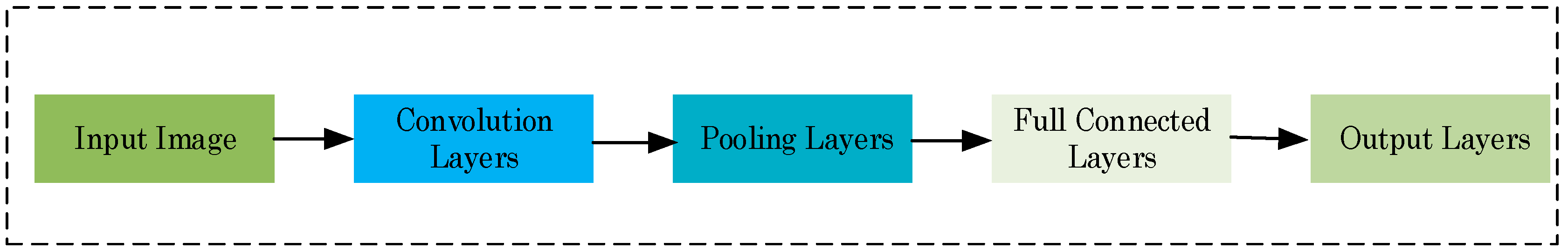
CNN is a multilayer perceptron inspired by the visual neural mechanism. Generally, a typical CNN architecture consists of the input layer, the convolution layer, the pooling layer, the full connection layer, and the output layer [19]. The first convolutional layer computes convolution of the input image with convolutional kernels [20]. The convolution layer is often followed by an activation function, after the pooling layer becomes the fully connected layer [21], as illustrated in Figure 2.
Generally, a convolution operator is followed by a transformation, called the ReLU function [22]. Suppose is the feature map of the th layer. Then, represents the weight feature vector of the th convolution kernel. Mathematically, the convolution process can be defined by the equation below [23].
where is the bias in the th channel. denotes a convolution operation of the th layer of the image and the th layer of the input data. is the activation function.
The ReLU function has recently been frequently used in literature due to neurons with rectified functions performing well to overcome saturation during the learning process [24]. The ReLU function can be defined by the equation below.
The pooling layer’s function is to merge semantically similar features into one. In general, typical pooling is the max-pooling and average-pooling [25]. Let us assume that is a feature map. The max pooling can be expressed by Equation (7)
where stand for describe as the max element from the feature map.
The average-pooling can be expressed by Equation (8)
where the size of the pooling area is pixels.
Image features loss is an inevitable problem with the subsampling (pooling) process. It always leads to low clouds and snow detection accuracy. We present self-adaptive pooling based on the maximum pooling and the average pooling. The self-adaptive pooling can adaptively adjust the pooling process through the pooling factors in the complex pooling area [26]. The self-adaptive pooling is shown by Equation (9) [27].
where is the pooling factor. The role of is to dynamically optimize both the max pooling and the average pooling based on different pooling blocks. The pooling factor can be defined by the equation below [28].
where is the average of all elements except for the max element in the pooling area and is the max element in the pooling area.
A fully connected layer causes overfitting due to these producing the many parameters. In general, to reduce overfitting, it weightily depends on dropout regularization and spatial dropout. The overfitting often leads to low classification accuracy with ineffective training tasks. However, Global Average Pooling (GAP) [29] does not require any optimization. Therefore, two patches-based CNN are replaced by fully connected layers with GAP.
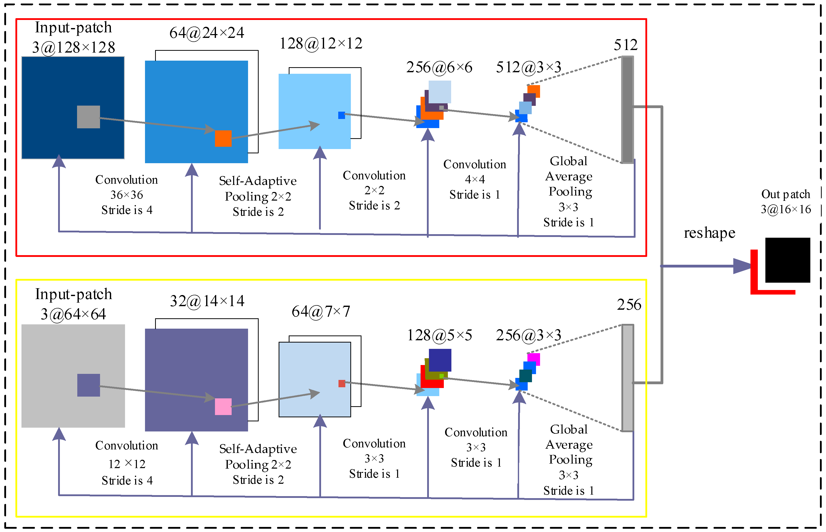
We design a new two patches CNN structure shown in Figure 3. In this study, we present a new two patches CNN architecture, which uses two branches (128 × 128 and 64 × 64) as the input data to mine multi-scale semantic features. The input patch size of 128 × 128 makes up the CNN structure (red box). The first convolution layer is 64@ 24 × 24 and it is composed of 64 filter channels with a dimension of 24 × 24, which is a result of the convolution of an input patch with the kernel of dimensions 36 × 36 with stride 4. Then, the first convolution layer is followed by a self-adaptive pooling of dimensions 2 × 2, which results in 128@ 12 × 12. This process is followed by convolution of 128@ 12 × 12 with filter-kernel of sizes 2 × 2 and 4 × 4 with filter units 256 and 512. Finally, the GAP is computed to 512 channels of dimension size 3 × 3 to reproduce 512@ 1 × 1.
For the input patch size of 64 × 64 for the CNN structure (yellow box), the first convolution layer is 32@ 14 × 14, which is a result of the convolution of an input patch with the dimension size 12 × 12 with stride 4. Then, the first convolution layer followed by self-adaptive pooling of the dimension size 2 × 2 results in 64@ 7 × 7. This process is followed by convolution of 64@ 7 × 7 with a filter-kernel of sizes 3 × 3 and filter units of 128 and 256. Lastly, the GAP is computed with 512 channels of dimension sizes 3 × 3 and reproduced 256@ 1 × 1. The rectified linear units (RELU) [30] are applied to the output of the every convolutional layer. The output is a 768-dimensional vector, which is reshaped into a 16 × 16 size of three channels (snow, cloud, and background). The softmax classifier is applied to the global average pooling, connected to the detection of snow and clouds.
2.3. Accuracy Assessment
The accuracy of the cloud and snow extraction used in this study were evaluated, which included Overall Accuracy (OA) and the Kappa. The cloud and snow in the study area were manually drawn in ENVI (Harris Geospatial, Boulder, CO, USA). Therefore, Overall Accuracy (OA) and the Kappa were used to assess the accuracy of the algorithm results. We used overall accuracy, which is the percentage of correctly classified cloud pixels. Take the cloud as an example. The OA and Kappa are defined as [31]:
where is the total number of pixels in the testing image; , , , and denote the pixels for the accurate extraction of cloud, missing cloud regions, inaccurate extraction cloud, and accurate rejection of background regions, respectively; and .
3. Experiment and Analysis
The new two patches CNN architecture is implemented by using Python 3.5 a PC with an I7 8086K CPU and GPU NVidia Tesla M40 with 12 GB of memory. Our CNN is implemented through the software library Tensorflow (Google Brain Team, Mountain View, CA, USA). The training dataset is manufactured from two SPOT-6 multispectral images and nine Gaofen-1 multispectral images. In the training dataset, 20,000 pairs of patches are obtained from the training set, where the number of clouds, snow, and background patches are 8000, 8000, and 4000, respectively. In this paper, we set up the weights in each layer with a random number drawn from a zero-mean Gaussian distribution with a standard deviation of 0.01. We used batch gradient descent with a mini-batch size of 768. The learning rate started from 0.001. The ground values of cloud and snow areas were manually extracted.
3.1. Performance of Improved Superpixel Method and Different CNN Architectures
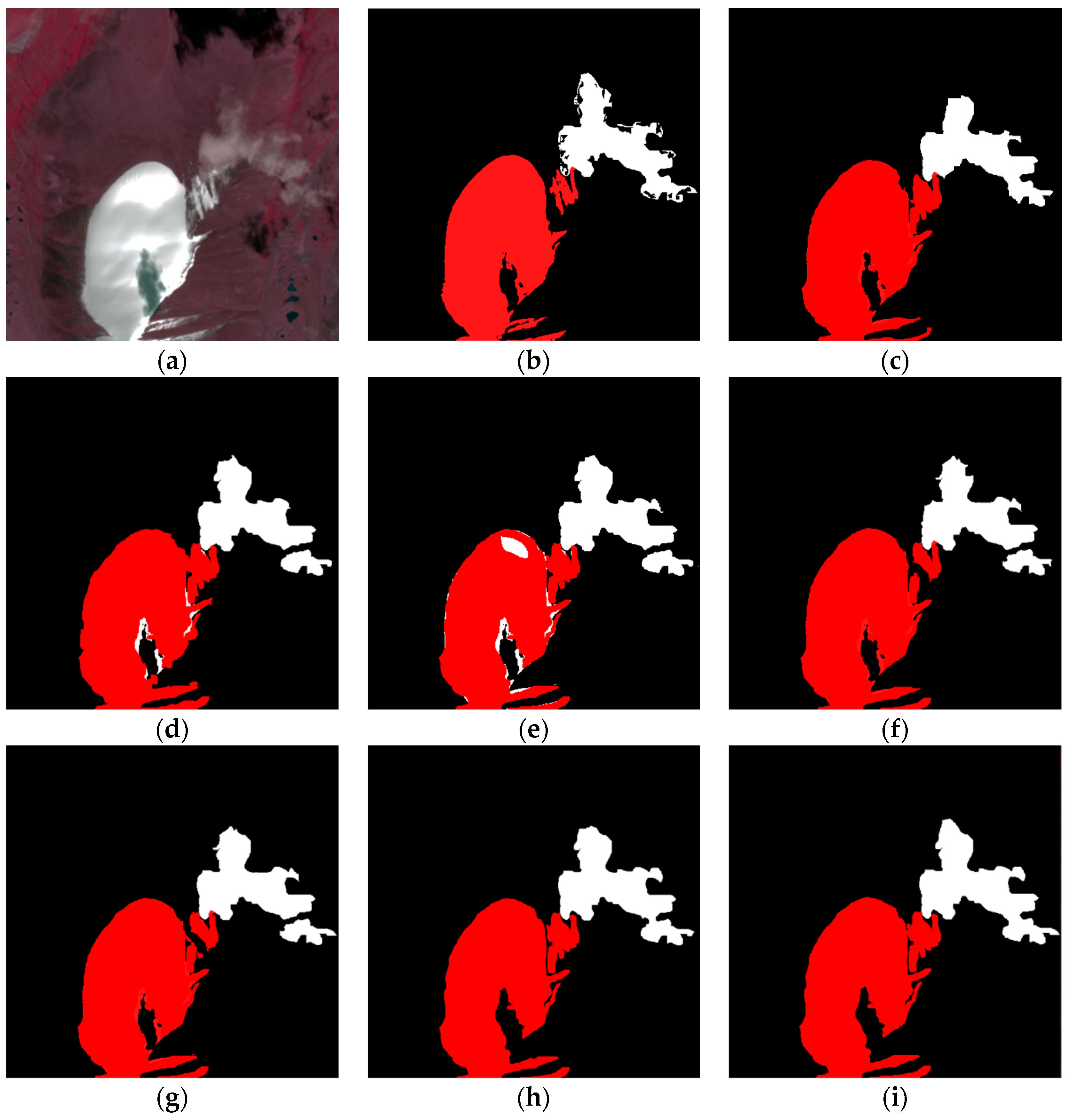
In order to verify the effectiveness of the improved SLIC method and double-branch CNN, we compared it with our double-branch CNN + pixel, our double-branch + SLIC, single-branch CNN (input branch size of 128 × 128, the first branch (red box) in Figure 3), single-branch CNN (input branch size of 64 × 64, the second branch (yellow box) in Figure 3), our double-branch + average pooling, and our double-branch + max pooling.
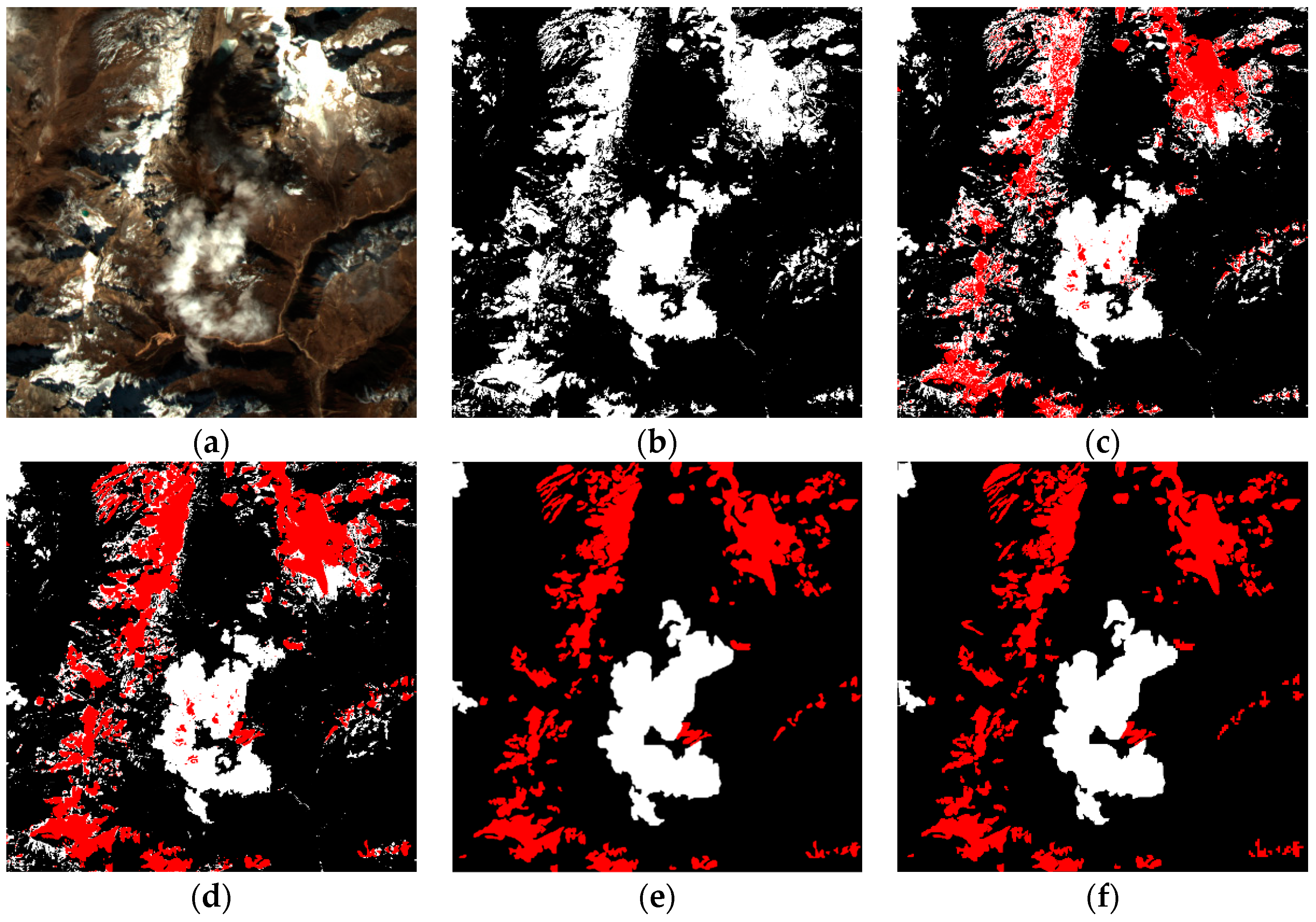
Based on the visual assessment, Figure 4 shows the visual performance of the improved superpixel method and different CNN structural methods at cloud and snow detection tasks. Compared with the truth situation, single-branch CNNs bring more false negatives and false positives than our double-branch CNNs Structures in cloud and snow detection, which can extract the multi-scale semantic features in input data. Among the CNN Structures, our CNN achieves better visual performance than CNN + max pooling and CNN + average pooling. From Figure 4b–h, the superpixel-level-based methods can avoid the disadvantage of the “salt-and-pepper” effect.
To evaluate the quantitative performance among different cloud and snow detection methods, the overall accuracy (OA) and Kappa Coefficient (Kappa) are used. Table 1 shows the statistical results.
As shown in Table 1, superpixel segmentation preprocessing further improved the accuracy of our method. The OA accuracy reached 95%, which demonstrates the effectiveness of double-branch CNN and superpixel oriented preprocessing. However, our proposed method achieves the best performance in the two metrics.
3.2. Comparison with Other Cloud and Snow Detection Algorithms
To verify the effectiveness of the proposed method, we compare it with the ENVI threshold method [32], ANN [33], and SVM [34].
Based on the visual assessment, Figure 5 shows the similar results using different cloud and snow detection methods. There are some limitations in the ENVI threshold cloud and snow detection. The ENVI threshold method may fail to separate the cloud from the snow (Figure 5b) in the Gaofen-1 multispectral image. Our proposed method can accurately separate the cloud and snow in the high-resolution image, and results are more accurate and robust compared to the other methods.
To evaluate the quantitative performance among different cloud and snow detection methods, the overall accuracy (OA) and Kappa Coefficient (Kappa) are used. The metric precision for ENVI threshold methods is not given in this paper because it could not separate the clouds from the snow. Table 2 shows the statistical OA and Kappa results.
From Table 2, our methods obtained high OA and a reasonable kappa coefficient, which verifies the feasibility and effectiveness of the cloud detection. In addition, the proposed method outperforms the ENVI threshold method, ANN, and SVM by a large margin. Specifically, the proposed method is about 33% (Kappa) higher than the ENVI threshold method for cloud detection.
4. Conclusions
Generally, it is not easy to separate clouds from snow when using high-resolution remote sensing imagery which only includes visible and near-infrared spectral bands. As a result of the insufficient spectral information for high-resolution remote sensing imagery for cloud and snow detection, they are difficult to capture. In this work, a new CNN architecture is proposed for cloud and snow detection on an object level. Specifically, a two patch-based deep CNN architecture is used, which can deeply mine multi-scale feature and semantic feature (including such areas as “building is surrounded by “building shadow”). The improved SLIC method was applied to segment the spectral image into shape regular superpixels, which were used to enhance our CNN outputs. The experimental results demonstrate that the proposed CNN architecture can accurately separate the clouds and snow. In addition, the extraction result is more feasible and effective than that of the traditional cloud detection algorithm.
In a future study, we could generalize the proposed convolutional neural network-based methods to another task in remote sensing fields such as urban water extraction and ship detection.
Author Contributions
L.W. responsible for the research design, experiment. Y.C. prepared the manuscript and interpreted the results. R.F. gave some advices in writing the paper. L.T. and Y.Y. has reviewed the paper. All authors reviewed the manuscript.
Funding
This work is partially supported by the China Postdoctoral Science Foundation (2017M621229), the Postdoctoral Science Foundation of Heilongjiang Province(LBH-Z17001), the National Natural Science Foundation of China for Young Scholars (41101177, 41301081), the China Scholarship Council (201708230012), the National Key Research and Development Plan of China (2017YFB0503604, 2016YFE0200400), the National Natural Science Foundation of China (41671442, 41571430, 41271442), and the Joint Foundation of Ministry of Education of China (6141A02022341).
Conflicts of Interest
The authors declare no conflict of interest.
References
- Kovalskyy, V.; Roy, D. A one year Landsat 8 conterminous United States study of cirrus and non-cirrus clouds. Remote Sens. 2015, 7, 564–578. [Google Scholar] [CrossRef]
- Xu, X.; Guo, Y.; Wang, Z. Cloud image detection based on Markov Random Field. J. Electron. (China) 2012, 29, 262–270. [Google Scholar] [CrossRef]
- Zhu, Z.; Woodcock, C.E. Object-based cloud and cloud shadow detection in Landsat imagery. Remote Sens. Environ. 2012, 118, 83–94. [Google Scholar] [CrossRef]
- Shen, H.F.; Li, H.F.; Qian, Y.; Zhang, L.P.; Yuan, Q.Q. An effective thin cloud removal procedure for visible remote sensing images. ISPRS J. Photogramm. Remote Sens. 2014, 96, 224–235. [Google Scholar] [CrossRef]
- Li, C.-H.; Kuo, B.-C.; Lin, C.-T.; Huang, C.-S. A spatial-contextual support vector machine for remotely sensed image classification. IEEE Trans. Geosci. Remote Sens. 2012, 50, 784–799. [Google Scholar] [CrossRef]
- Lasota, E.; Rohm, W.; Liu, C.-Y.; Hordyniec, P. Cloud detection from radio occultation measurements in tropical cyclones. Atmosphere 2018, 9, 418. [Google Scholar] [CrossRef]
- Hansen, M.C.; Roy, D.P.; Lindquist, E.; Adusei, B.; Justice, C.O.; Altstatt, A. A method for integrating MODIS and Landsat data for systematic monitoring of forest cover and change in the Congo basin. Remote Sens. Environ. 2008, 112, 2495–2513. [Google Scholar] [CrossRef]
- Huang, C.Q.; Thomas, N.; Goward, S.N.; Masek, J.G.; Zhu, Z.L.; Townshend, J.R.G.; Vogelmann, J.E. Automated masking of cloud and cloud shadow for forest change analysis using Landsat images. Int. J. Remote Sens. 2010, 31, 5449–5464. [Google Scholar] [CrossRef]
- Zhu, Z.; Woodcock, C.E. Automated cloud, cloud shadow, and snow detection in multitemporal Landsat data: An algorithm designed specifically for monitoring land cover change. Remote Sens. Environ. 2014, 152, 217–234. [Google Scholar] [CrossRef]
- Hall, D.K.; Riggs, G.A.; Salomonson, V.V. Development of methods for mapping global snow cover using moderate resolution imaging spectroradiometer data. Remote Sens. Environ. 1995, 54, 127–140. [Google Scholar] [CrossRef]
- Alireza, T.; Fabio, D.F.; Cristina, C.; Stefania, V. Neural networks and support vector machine algorithms for automatic cloud classification of whole-sky ground-based images. IEEE Trans. Geosci. Remote Sens. 2015, 12, 666–670. [Google Scholar]
- Achanta, R.; Shaji, A.; Smith, K.; Lucchi, A.; Fua, P.; Süsstrunk, S. SLIC superpixels compared to state-of-the-art superpixel methods. IEEE Trans. Pattern Anal. Mach. Intell. 2012, 34, 2274–2282. [Google Scholar] [CrossRef] [PubMed]
- Csillik, O. Fast Segmentation and classification of very high resolution remote sensing data using SLIC superpixels. Remote Sens. 2017, 9, 243. [Google Scholar] [CrossRef]
- Zhang, G.; Jia, X.; Hu, J. Superpixel-based graphical model for remote sensing image mapping. IEEE Trans. Geosci. Remote Sens. 2015, 53, 5861–5871. [Google Scholar] [CrossRef]
- Hagos, Y.B.; Minh, V.H.; Khawaldeh, S.; Pervaiz, U.; Aleef, T.A. Fast PET scan tumor segmentation using superpixels, principal component analysis and K-Means clustering. Methods Protoc. 2018, 1, 7. [Google Scholar] [CrossRef]
- Li, H.; Shi, Y.; Zhang, B.; Wang, Y. Superpixel-based feature for aerial image scene recognition. Sensors 2018, 18, 156. [Google Scholar] [CrossRef] [PubMed]
- Zhang, F.; Du, B.; Zhang, L. Scene classification via a gradient boosting random convolutional network ramework. IEEE Trans. Geosci. Remote Sens. 2016, 54, 1793–1802. [Google Scholar] [CrossRef]
- Mateo-García, G.; Gómez-Chova, L.; Amorós-López, J.; Muñoz-Marí, J.; Camps-Valls, G. Multitemporal cloud masking in the Google Earth Engine. Remote Sens. 2018, 10, 1079. [Google Scholar] [CrossRef]
- Dong, C.; Loy, C.C.; He, K.; Tang, X. Learning deep convolutional networks for image super resolution. In Proceedings of the European Conference on Computer Vision, Athens, Greece, 11–13 November 2015. [Google Scholar]
- Pouliot, D.; Latifovic, R.; Pasher, J.; Duffe, J. Landsat super-resolution enhancement using convolution neural networks and Sentinel-2 for training. Remote Sens. 2018, 10, 394. [Google Scholar] [CrossRef]
- Scarpa, G.; Gargiulo, M.; Mazza, A.; Gaetano, R. A CNN-based fusion method for feature extraction from Sentinel data. Remote Sens. 2018, 10, 236. [Google Scholar] [CrossRef]
- Chen, F.; Ren, R.; Van de Voorde, T.; Xu, W.; Zhou, G.; Zhou, Y. Fast automatic airport detection in remote sensing images using convolutional neural networks. Remote Sens. 2018, 10, 443. [Google Scholar] [CrossRef]
- Hu, F.; Xia, G.-S.; Hu, J.; Zhang, L. Transferring deep convolutional neural networks for the scene classification of high-resolution remote sensing imagery. Remote Sens. 2015, 7, 14680–14707. [Google Scholar] [CrossRef]
- Mboga, N.; Persello, C.; Bergado, J.R.; Stein, A. Detection of informal settlements from VHR images using convolutional neural networks. Remote Sens. 2017, 9, 1106. [Google Scholar] [CrossRef]
- Guo, Z.; Chen, Q.; Wu, G.; Xu, Y.; Shibasaki, R.; Shao, X. Village building identification based on ensemble convolutional neural networks. Sensors 2017, 17, 2487. [Google Scholar] [CrossRef] [PubMed]
- Xu, Y.; Wu, L.; Xie, Z.; Chen, Z. Building extraction in very high-resolution remote sensing imagery using deep learning and guided filters. Remote Sens. 2018, 10, 144. [Google Scholar] [CrossRef]
- Chen, Y.; Fan, R.; Yang, X.; Wang, J.; Latif, A. Extraction of urban water bodies from high-resolution remote-sensing imagery using deep learning. Water 2018, 10, 585. [Google Scholar] [CrossRef]
- Chen, Y.; Fan, R.; Bilal, M.; Yang, X.; Wang, J.; Li, W. Multilevel cloud detection for high-resolution remote sensing imagery using multiple convolutional neural networks. ISPRS Int. J. Geo-Inf. 2018, 7, 181. [Google Scholar] [CrossRef]
- Zhao, W.; Guo, Z.; Yue, J.; Zhang, X.; Luo, L. On combining multiscale deep learning features for the classification of hyperspectral remote sensing imagery. Int. J. Remote. Sens. 2015, 36, 3368–3379. [Google Scholar] [CrossRef]
- Ren, S.; He, K.; Girshick, R.; Sun, J. Faster R-CNN: Towards real-time object detection with region proposal networks. IEEE Trans. Pattern Anal. Mach. Intell. 2017, 39, 1137–1149. [Google Scholar] [CrossRef] [PubMed]
- Congalton, R.G.; Green, K. Assessing the Accuracy of Remotely Sensed Data: Principles and Practices; Lewis Publications (CRC Press): Boca Raton, FL, USA, 1999. [Google Scholar]
- Marais, I.V.Z.; Du Preez, J.A.; Steyn, W.H. An optimal image transforms for threshold-based cloud detection using heteroscedastic discriminant analysis. Int. J. Remote Sens. 2011, 32, 1713–1729. [Google Scholar] [CrossRef]
- Kussul, N.; Skakun, S.; Kussul, O. Comparative analysis of neural networks and statistical approaches to remote sensing image classification. Int. J. Comput. 2014, 5, 93–99. [Google Scholar]
- Wang, H.; He, Y.; Guan, H. Application support vector machines in cloud detection using EOS/MODIS. In Proceedings of the Remote Sensing Applications for Aviation Weather Hazard Detection and Decision Support, San Diego, CA, USA, 25 August 2008. [Google Scholar]
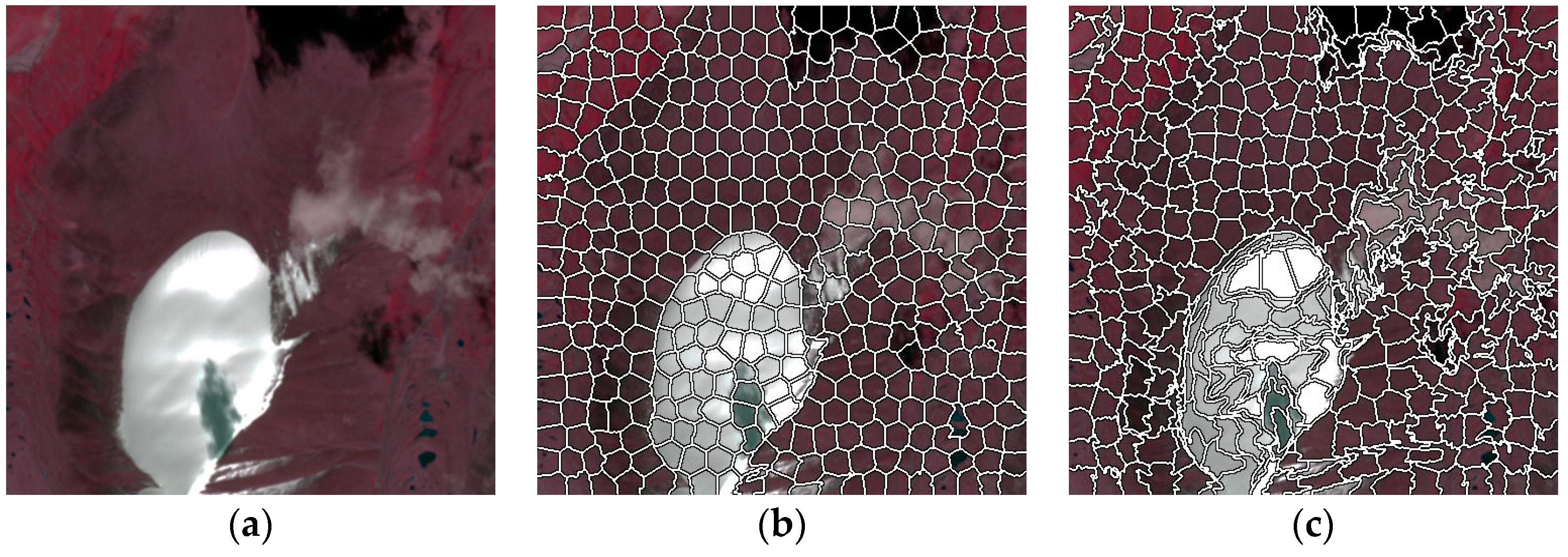
Figure 1.
Superpixel segmentation instance: (a) Original image; (b) The improved SLIC; (c) Regular-SLIC.
Figure 1.
Superpixel segmentation instance: (a) Original image; (b) The improved SLIC; (c) Regular-SLIC.

Figure 2.
The standard architecture of the CNNs.

Figure 3.
The architecture of the used CNNs.

Figure 4.
Cloud and snow detection results using different superpixel segmentation and different CNNs. Red area: Snow. White area: Cloud. Black area: Background. (a) SPOT-6 multispectral image. (b) Our double-branch CNN + pixel. (c) Our double-branch CNN + SLIC. (d) Single-branch CNN (input branch size of 128 × 128). (e) Single-branch CNN (input branch size of 64 × 64). (f) Our double-branch CNN + average pooling. (g) Our double-branch CNN + max pooling. (h) Our proposed framework. (i) Ground truth.

Figure 5.
Visual comparison among different comparing methods. Red area: Snow. White area: The cloud. Black area: Background. (a) Gaofen-1 multispectral image. (b) ENVI threshold method. (c) ANN. (d) SVM. (e) Our proposed framework. (f) Ground truth.
Figure 5.
Visual comparison among different comparing methods. Red area: Snow. White area: The cloud. Black area: Background. (a) Gaofen-1 multispectral image. (b) ENVI threshold method. (c) ANN. (d) SVM. (e) Our proposed framework. (f) Ground truth.


Table 1.
Results on the SPOT-6 multispectral images for different methods in terms of OA and Kappa.
| Method | Cloud | Snow | ||
|---|---|---|---|---|
| OA (%) | Kappa (%) | OA (%) | Kappa (%) | |
| Our double-branch CNNs + pixel | 93.46 | 89.17 | 94.36 | 89.51 |
| Our double-branch CNNs + SLIC | 95.31 | 90.14 | 96.81 | 90.51 |
| CNNs (input branch size of 128 × 128) | 92.29 | 88.94 | 90.97 | 88.37 |
| CNNs (input branch size of 64 × 64) | 90.38 | 88.97 | 88.19 | 88.47 |
| double-branch CNNs + average pooling | 95.71 | 89.81 | 95.96 | 90.01 |
| Our double-branch CNNs + max pooling | 96.14 | 91.27 | 96.91 | 91.52 |
| Our proposed framework | 98.36 | 92.64 | 99.17 | 93.27 |
Table 2.
Quantitative comparison among different methods.
| Method | Cloud | Snow | ||
|---|---|---|---|---|
| OA (%) | Kappa (%) | OA (%) | Kappa (%) | |
| ENVI threshold method | 68.34 | 59.74 | / | / |
| ANN | 76.69 | 69.17 | 71.94 | 68.35 |
| SVM | 79.19 | 70.39 | 80.39 | 70.94 |
| Our proposed framework | 99.16 | 92.64 | 98.17 | 92.97 |
© 2018 by the authors. Licensee MDPI, Basel, Switzerland. This article is an open access article distributed under the terms and conditions of the Creative Commons Attribution (CC BY) license (http://creativecommons.org/licenses/by/4.0/).
Share and Cite
MDPI and ACS Style
Wang, L.; Chen, Y.; Tang, L.; Fan, R.; Yao, Y. Object-Based Convolutional Neural Networks for Cloud and Snow Detection in High-Resolution Multispectral Imagers. Water 2018, 10, 1666. https://doi.org/10.3390/w10111666
AMA Style
Wang L, Chen Y, Tang L, Fan R, Yao Y. Object-Based Convolutional Neural Networks for Cloud and Snow Detection in High-Resolution Multispectral Imagers. Water. 2018; 10(11):1666. https://doi.org/10.3390/w10111666
Chicago/Turabian StyleWang, Lei, Yang Chen, Luliang Tang, Rongshuang Fan, and Yunlong Yao. 2018. "Object-Based Convolutional Neural Networks for Cloud and Snow Detection in High-Resolution Multispectral Imagers" Water 10, no. 11: 1666. https://doi.org/10.3390/w10111666
Note that from the first issue of 2016, this journal uses article numbers instead of page numbers. See further details here.