Assessment of Machine Learning Techniques for Monthly Flow Prediction


1
Faculty of Civil, Water and Environmental Engineering, Shahid Beheshti University, Tehran 16589-53571, Iran
2
School of Civil, Environmental, and Architectural Engineering, Korea University, Seoul 136-713, Korea
*
Author to whom correspondence should be addressed.
Water 2018, 10(11), 1676; https://doi.org/10.3390/w10111676
Submission received: 11 October 2018
/
Revised: 9 November 2018
/
Accepted: 14 November 2018
/
Published: 17 November 2018
(This article belongs to the Special Issue Machine Learning Applied to Hydraulic and Hydrological Modelling)
Abstract
:Monthly flow predictions provide an essential basis for efficient decision-making regarding water resource allocation. In this paper, the performance of different popular data-driven models for monthly flow prediction is assessed to detect the appropriate model. The considered methods include feedforward neural networks (FFNNs), time delay neural networks (TDNNs), radial basis neural networks (RBFNNs), recurrent neural network (RNN), a grasshopper optimization algorithm (GOA)-based support vector machine (SVM) and K-nearest neighbors (KNN) model. For this purpose, the performance of each model is evaluated in terms of several residual metrics using a monthly flow time series for two real case studies with different flow regimes. The results show that the KNN outperforms the different neural network configurations for the first case study, whereas RBFNN model has better performance for the second case study in terms of the correlation coefficient. According to the accuracy of the results, in the first case study with more input features, the KNN model is recommended for short-term predictions and for the second case with a smaller number of input features, but more training observations, the RBFNN model is suitable.
1. Introduction
Future river discharge predictions have been widely used for flood control, drought protection, reservoir management, and water allocation. However, it is difficult to develop an exact physically based mathematical model to express the relationship between flow discharge and future forecasted precipitations, due to various uncertainties. Owing to a lack of adequate knowledge regarding the physical processes in the hydrologic cycle, traditional statistical models, such as the auto regressive moving average (ARMA) and auto regressive integrated moving average (ARIMA) models [1], have been developed to predict and generate synthetic data. Nevertheless, such models do not attempt to represent the nonlinear dynamics inherent to the hydrological process, and may not always perform well [2]. During the past few decades, artificial neural networks have gained considerable attention for time series predictions [3]. ANNs have been successfully applied to river level predictions and flood forecasting [4,5], daily flow forecasting [6], rainfall-runoff modeling and short-term forecasting [7], and monthly flow predictions [8]. The main advantage of using an ANN instead of a conventional statistical approach is that an ANN does not require information on the complex nature of the hydrological process under consideration to be explicitly described in a mathematical form. However, ANN models suffer from overfitting or overtraining, which decreases the capability of the prediction for data far from the training samples.
Another machine learning algorithm that appears to be successful in hydrological predictions is support vector machine (SVM), which is also called support vector regression (SVR) when applied to function approximation or time series predictions. SVMs have been successfully applied to time series forecasting [9], the stock market [10] and in particular, water-related applications for the prediction of wave height [11]), the generation of operating rules for reservoirs [12], drought monitoring [13], water level prediction [14], and short- and long-term flow forecasting [15], among others. Overfitting and local optimal solution are unlikely to occur with an SVM, and this enhances the performance of SVM for the prediction. A major challenge in the application of the SVM method is the tuning of the parameters of the model and kernels, which severely affects the accuracy of the results [16]. Applying SVR model in combination with other machine learning models can lead to more accurate predictions [16,17] or discharge estimations at ungauged sites [18]. For this study, a grasshopper optimization algorithm (GOA) [19] is used and combined with the SVM to enhance the ability of the machine for river-flow predictions.
KNN is another data-driven method, a simple, but efficient, method to model monthly flow [20] and daily inflow [21].
The main contribution of this paper is the assessment of different soft-computing methods in a unified platform along with applying Gaussian process regression (GPR) and GOA-SVR models for predicting monthly river discharge as the basis of reservoir management. To evaluate the efficiency of the proposed models, two study area with different input variables are chosen. In the first study area, the input data set involves monthly discharge and temperature, each with three temporal lags, which belong to a period of 18-years (from 1983 to 2004) and in another case study, there are three input variables, including river discharge of three temporal lags which have been observed monthly during 40 years (from 1962 to 1990). The results obtained were compared with those found by different types of artificial neural networks, including feedforward neural networks (FFNNs), time delay neural networks (TDNNs), radial basis neural networks (RBFNNs), recurrent neural networks (RNNs), and a KNN model. The remainder of this paper is organized as follows. In Section 2, a brief description of the models and their concepts, including the GPR, SVR, GOA, ANN configurations, and KNN, are represented. The case studies used, and their characteristics, are then illustrated in Section 3. In Section 4, the models are applied to time series predictions for the two case studies, and the performance of the models is compared in terms of statistical metrics. Finally, Section 5 offers some concluding remarks and future research issues.
2. Materials and Methods
There are many textbooks and scientific papers in the literature that provide a detailed description of GPR [22], SVM [23,24], neural networks, and their variants [25] in terms of both theory and application. Hence, in this paper, only a brief description of the applied techniques is given.
2.1. Gaussian Process Regression
Gaussian process regression (GPR) as a statistical method, is a generalization of the Gaussian probability distribution. This method is described as follows:
Consider a training dataset with n observations where is the input variable and is the target. The principal goal is the estimation of output value corresponding to the new (test) input . In the Gaussian process regression, it is assumed that the observations are noisy as where is a regression function approximated by a Gaussian process with the corresponding mean that is often null and the covariance (or kernel) function . Also, is the noise that follows a Gaussian distribution . Thus, the form of GPR model is as follows:
Considering the properties of Gaussian distribution, the marginal distribution of can be defined as:
where, is the input data set, is the set of target values and is the value of the stochastic function f calculated for each input variable. There is a joint distribution between outputs and as below:
where , , and are the test data set, testing outputs, and identity matrix, respectively. In addition, , and are covariance matrices. The covariance function plays an important role in a Gaussian process regression to specify the similarity among data. There are several types of covariance functions; some of the most useful ones are written in the following:
- Squared exponential: ;
- Exponential: ;
- -exponential: ;
- Rational quadratic: ;
- Matern 3/2: ;
- Matern 5/2: .
where is the noise variance; (the length scale parameter), (the signal standard deviation), and are the parameters to be learned. The marginal likelihood is defined according to the Equation (7), where is the prior and is the likelihood. The log prior is defined as Equation (8), and the final log marginal likelihood is obtained as Equation (9):
According to the conditional distribution, the prediction process in GP regression for a given test data can be stated as:
where and are considered as posterior mean and covariance functions, respectively and defined as:
For more details on GPR algorithm, the reader is referred to [22].
2.2. SVR
Support Vector Machine is employed as a regression method in which a function is applied to discover the relationship between input and output variables, and , respectively.
where mapping the input vector into a high dimensional space is performed by non-linear transfer functions, ϕ(x). The most important feature of this space is the possibility of using a simple linear regression function. W is a coefficient vector and b represents a bias term.
A set of training data are employed to determine f(x) by calculating W and b. Then, the obtained coefficients are used to minimize the error function as below equations:
Subject to:
In the training process, the occurrence of the training error is inevitable. Therefore, a penalty term must be considered which is demonstrated by C. and N are the kernel function, and the number of samples, respectively. Moreover, are two indices of slack variables. stands for loss function related to the accuracy of the training process.
Finally, the SVR function can be rewritten as:
where are Lagrangian coefficients, is the kernel function. In the following, there is a number of these functions
- linear,
- polynomial,
- radial basis function (RBF) or Gaussian,
- sigmoid,
- quadratic,
The best SVR parameter values are often selected through a grid search with exponentially growing sequences of parameter values [23]. Another approach is applying an optimization algorithm. In this paper, GOA is applied to identify optimal values for the SVR parameters. The main steps of this algorithm are briefly described in the following section. The details of the SVR algorithm can be found in [23,24].
It is worth noting that there is a relationship between GPR and SVR algorithms. In order to obtain the maximum a posteriori margin (MAP) value of , presented in Equation (8), the below equation must be minimized:
On the other hand, by kernelizing Equation (13), the objective function can be stated as:
As can be seen, these two optimization problems are similar and by using a particular kernel and likelihood function in GPR model, the SVR model can be derived [22].
GOA Algorithm
The grasshopper optimization algorithm developed by Saremi et al. [19] is one of the recent algorithms inspired by grasshopper swarm behavior in nature. Grasshoppers, the insects moving in a network to find food, have a social interaction that leads to one of two type forces: Opposite forces and attraction forces that make possible global and local search, respectively. There is an area called comfort zone, where there is a balanced state between these forces such that they neutralize each other.
To reach the network target, in each step, grasshoppers move in the way so that their position is at the least spatial distance from the target while there must be a balance between local search and global search. Ultimately, after repeating the search steps, grasshoppers meet the optimum position. The mathematical structure of the grasshopper optimization algorithm is as follows:
where:
- : the d-dimensional position of the ith grasshopper in the iteration t;
- G: the number of grasshoppers;
- s: an evaluation function of social interactions;
- l: the attractive length scale;
- : the upper bound in the d-dimensional functions;
- : the lower bound in the d-dimensional functions;
- : the distance between the ith and jth grasshoppers;
- : is the d-dimensional position of the optimum solution found;
- c: the reduction factor to decrease the comfort zone;
In this algorithm, three agents have influences on the new place of each grasshopper: Its current location, the target point, and the situation of other grasshoppers.
2.3. Artificial Neural Networks
Artificial Neural Networks (ANNs) are highly flexible tools commonly used for function approximation and time series predictions. ANNs are typically a collection of neurons with a specific architecture constructed based on the relationship among neurons at different layers. This relatively complex architecture provides a nonlinear mapping from the input to the output space that can be used for a time series prediction. A typical problem of neural networks is overfitting or overtraining of the network arising from the “conformability” of the model structure with the shape of the available data. Overfitting decreases the generalization ability of ANN and degrades the accuracy level of the approximation model for data away from the training data. In this study, the early stopping approach [26] is used to avoid overtraining of ANN models. It is worth pointing out that this approach requires consistent data availability, and its application is not suggested in cases with sparse data where some alternative methods have better performance. In this technique, the available data are divided into three subsets. The first subset is the training set, which is used for computing the gradient and updating the network weights and biases. The second subset is the validation set. The error in the validation set is monitored during the training process. The validation error normally decreases during the initial phase of training, as does the training set error. However, when the network begins to overfit the data, the error in the validation set typically begins to increase. When the validation error increases for a specified number of iterations, the training is stopped, and the weights and biases at the minimum of the validation error are returned. The test set error is not used during training but is used to verify the generalization capability of the ANN model after training.
Based on the configuration of the network elements, different types of neural networks have been developed, and in this study, three commonly used ANNs, i.e., feedforward NNs, time delay NNs, and radial base NNs were chosen for monthly flow predictions. These networks are briefly described in the following section.
2.3.1. Feedforward Neural Networks
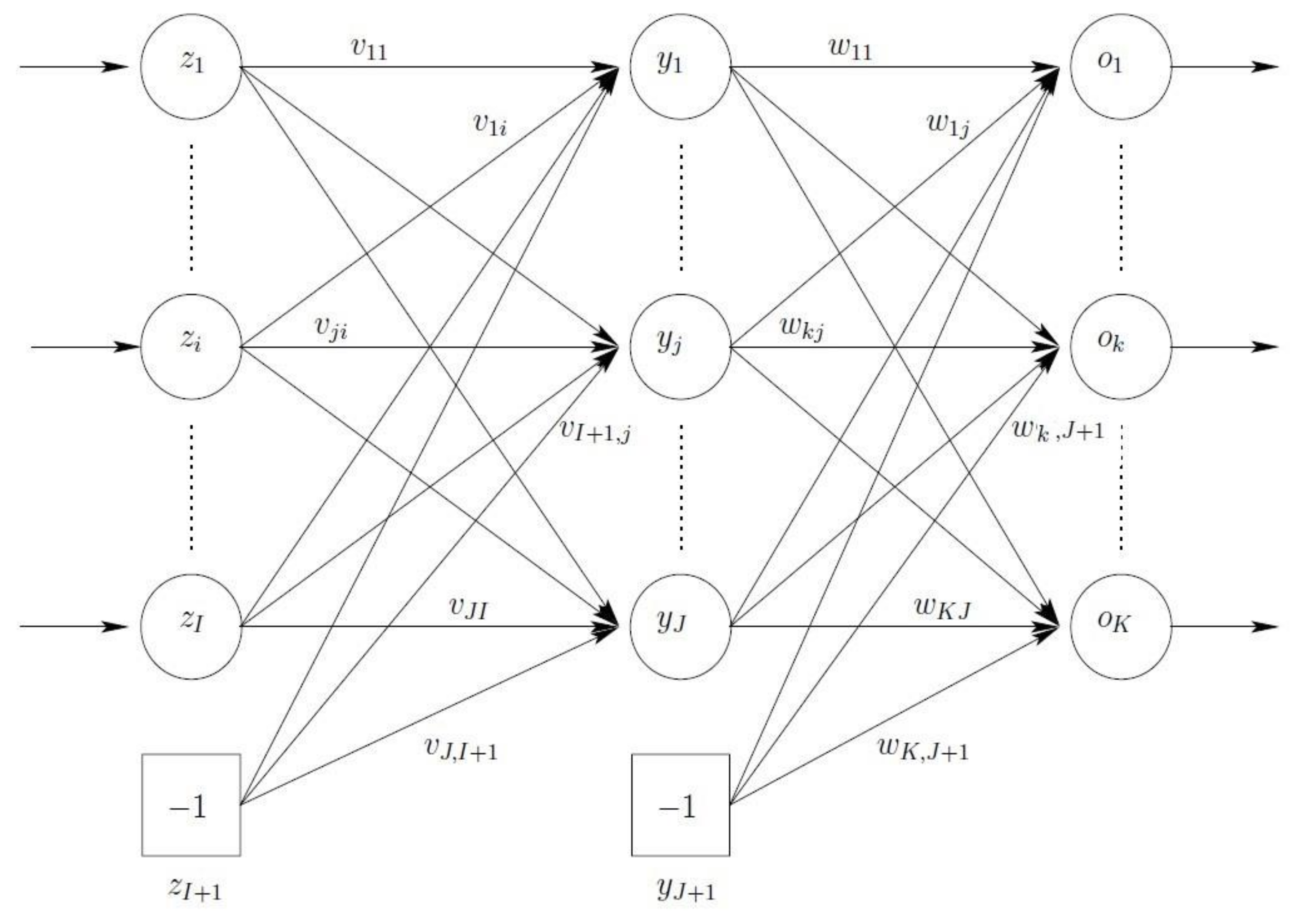
Feedforward neural networks (FFNNs) in this paper refer to multilayer perceptrons (NN-MLPs), which are by far the most popular type of neural networks [27]. Figure 1 illustrates a standard FFNN consisting of three layers: An input layer (note that sometimes an input layer is not counted as a layer), a hidden layer, and an output layer.
As shown in this figure, the output of an FFNN for any given input pattern zp is calculated with a single forward pass through the network. For each output unit ok, we have
where and are the activation function for output unit ok and hidden unit yj, respectively, wkj is the weight between output unit ok and hidden unit yj, and zi,p is the value of input unit zi of input pattern zp. In addition, the (I + 1)-th input unit and the (J + 1)-th hidden unit are bias units, representing the threshold values of neurons in the next layer.
FFNNs with one sigmoidal hidden layer and a linear output layer have been proven capable of approximating any function with any desired accuracy if the associated conditions are satisfied [28].
In this study, a two-layer feedforward neural network (one hidden layer and one output layer) is used for predicting monthly flows. The number of neurons in the hidden layer, along with the weights and biases, are obtained, based on the errors in the predicted values. Sigmoid and linear activation functions are used for the hidden layer and output layer, respectively. The weights and biases of the network are obtained using a back propagation Levenberg-Marquardt algorithm. After tuning the weights and testing the network, it is used for the prediction.
2.3.2. Radial Basis Neural Network
Radial basis neural networks are referred to as networks that, in contrast to conventional neural networks use regression-based methods and are not inspired by the biological neural system [29]. They work best when many training vectors are available [30]. A radial basis function (RBF) neural network (RBFNN) is an FFNN in which hidden units do not implement an activation function, but represent a radial basis function. An RBFNN approximates the desired function through the superposition of non-orthogonal, radially symmetric functions. An RBF is a three-layer network, with only one hidden layer. The output of each hidden unit is calculated as follows:
where represents the center of the basis function, and is the Euclidean norm. The output of an RBFNN is calculated as
2.3.3. Time Delay Neural Networks
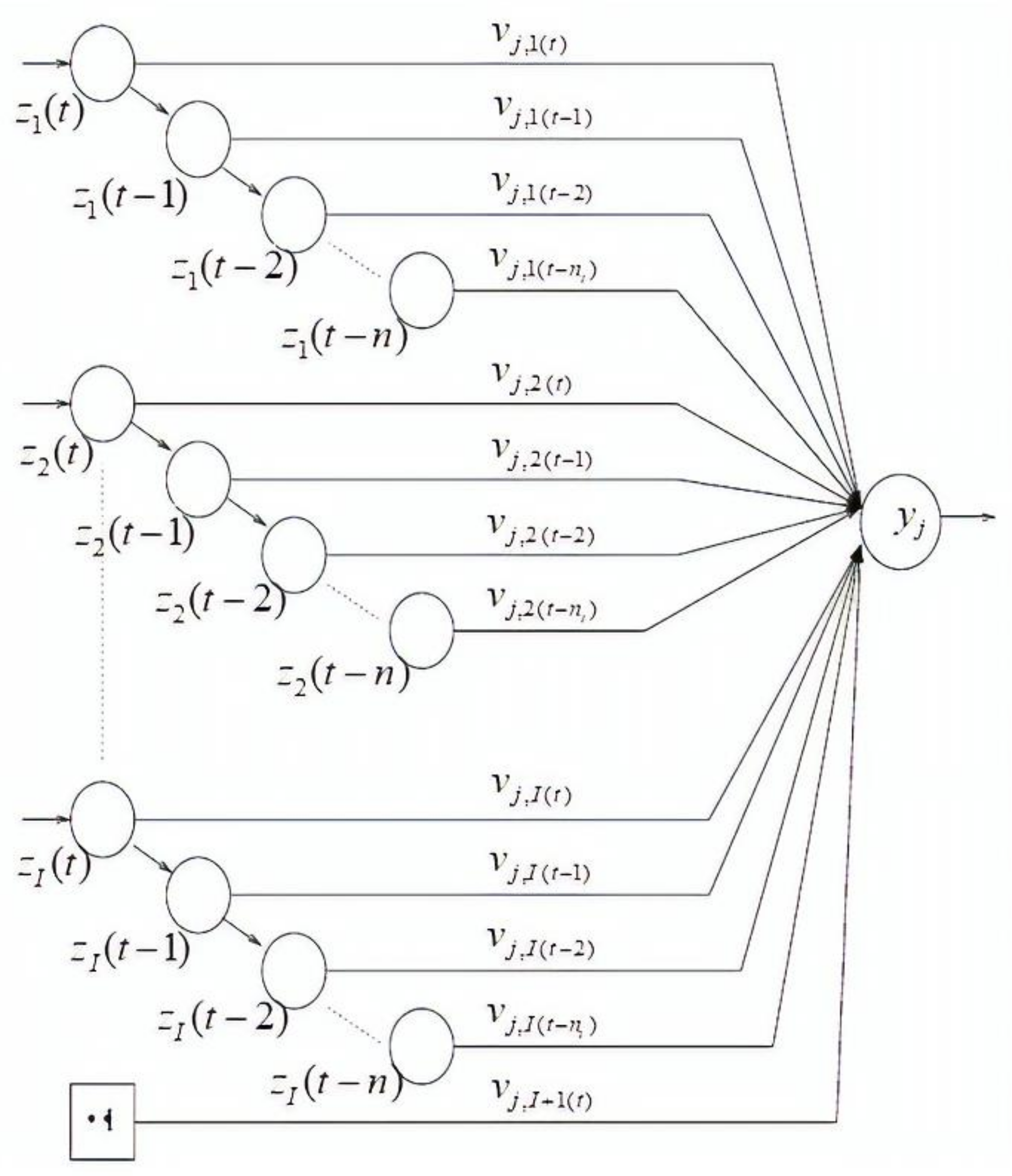
MLP neural networks only process input patterns that are spatial in nature, i.e., input patterns that can be arranged along one or more spatial axes, such as a vector or an array [30]. In many tasks, such as a time series prediction, the input pattern comprises one or more temporal signals. Time-delay neural networks (TDNNs) are of the dynamic neural network configurations that can handle temporal patterns of data. A TDNN [31] is a temporal network in that its input patterns are successively delayed over time. A single neuron with nt time delays for each input unit is illustrated in Figure 2. The output of a TDNN is calculated as follows:
2.3.4. Recurrent Neural Network
This section is intended for recurrent neural network (RNN) description. RNNs have a feedback loop to enhance the ability to learn from data sets. A simple type of these networks is schematized in Figure 3. As shown, outputs of the hidden layer, before entering to the output layer, are considered as new inputs with weights equal 1, to the (first) hidden layer. The input vector is therefore [25]:
Context units zI+2,…, zI+1+J are connected to all hidden units yj (for j = 1, · · ·, J) with a weight equal to 1. Thus, the activation value yj is simply copied to zI+1+j. Each output unit’s activation is then calculated as [25]:
where (zI+2,p, …, zI+1+J,p) = (y1,p(t−1), …, yJ,p(t−1)).
2.4. KNN Model
K-nearest neighbor (KNN) method, one of the nonparametric regression methods, utilizes the own data set to estimate the unknown variables applying the data in the nearest neighbor. Each of the close neighbors, the participants in the estimation process, has own weight which is determined based on its Euclidean distance from the unknown variable. The KNN formulation is presented as:
where is the amount of the unknown variable, is the neighbors’ values in the estimation process, is the Euclidean distance between known and unknown variables, and is the weight of each neighbor in the estimation process determined as follows:
Since, the number of diverse neighbors, leads to different results, it is important to find the best number of neighbors. Here, the choice of the various number of neighbors leads to relatively similar accuracy and the optimal value of K, considered as 7, has been obtained through a trial and error process with an accuracy of in terms of the correlation coefficient.
For the Alavian Basin, both the temperature and discharge data are available from the recorded data from Maragheh Station. Therefore, the monthly discharges and temperatures with three temporal lags, i.e., Q(t − 2), Q(t − 1), Q(t), T(t − 2), T(t − 1), and T(t), are considered as input variables to predict the next month’s discharge of the river, Q(t + 1), as the output variable. To assess the performance of the models, the observed time series datasets were divided into two independent subsets, namely, training and verification subsets. The training sets were used to learn the GPR, the SVR, and ANNs for prediction, whereas the verification sets were used to verify the ability of the models for prediction. The dataset from June 1983 to November 1996 (75% of the data) was selected for training, whereas that from December 1996 to June 2001 (the remaining 25%) was used for verification.
3. Case Studies
In this paper, two different study areas in Iran were considered to analyze the capabilities of the developed techniques in the prediction of monthly river flows.
3.1. Alavian Basin
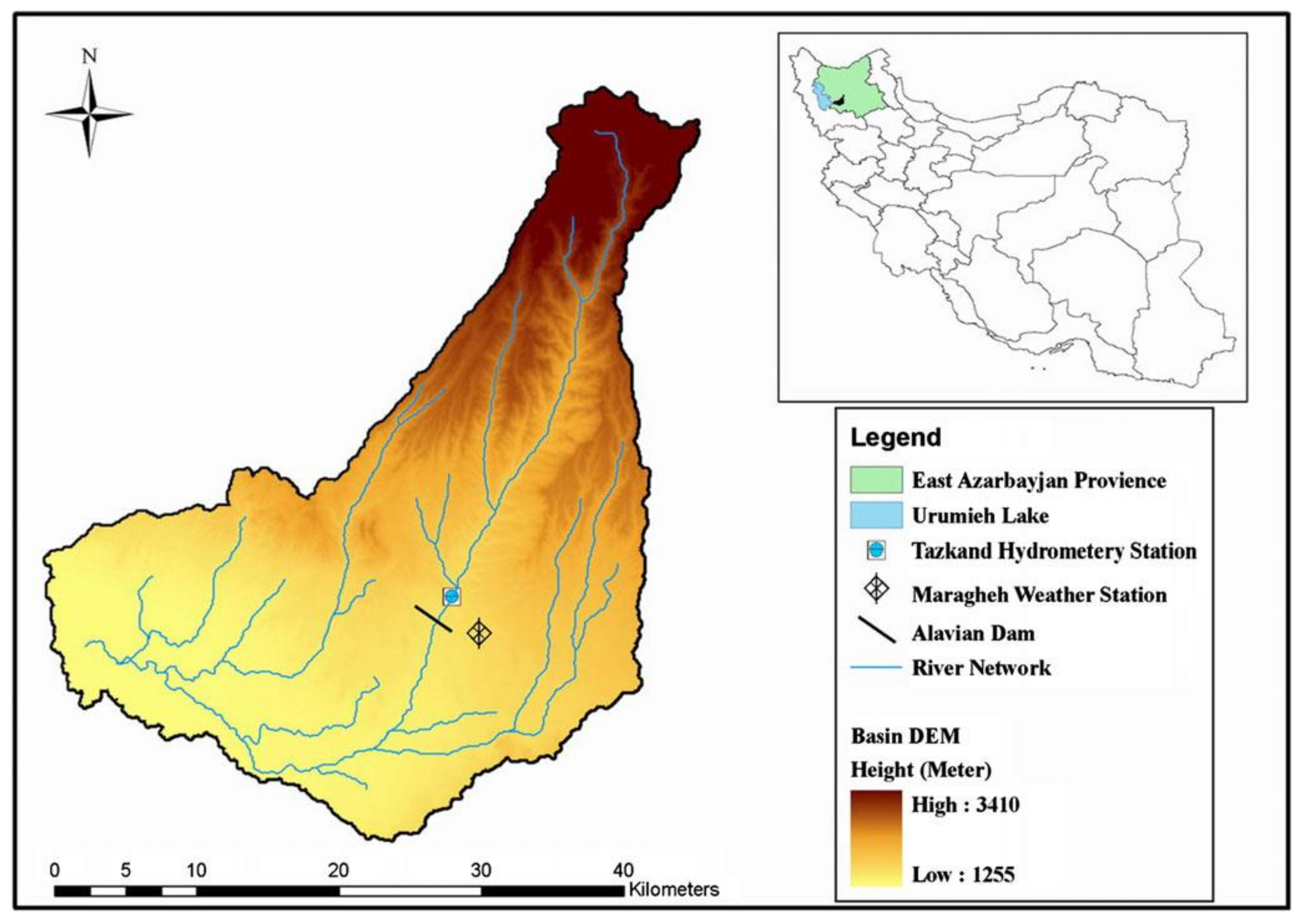
The first study region is Alavian Basin with an area of 239.10 km2 in the northwest part of Iran (Figure 4). Sufichay River is the main stream of the basin, which ends at Erumiyeh Lake. This river also constitutes the main inflow discharges to Alavian Dam, and its average annual discharge is estimated to be around 4.6 MCM. For this area, weather information, including the average precipitation and temperature at a monthly scale for an 18-year period (from 1983 to the end of 2001), were gathered from the Maragheh weather station, and monthly flow discharges were provided using the historical records of the Tazkand hydrometric station upstream of Alavian Dam. Owing to the snow melting in this basin, the monthly flow data can be a function of seasonal variations, and thus all gathered information, including monthly discharges and temperatures, each with three temporal lags, were considered as the inputs of the models (six input variables) for predicting the monthly flows. Figure 4 also shows the status of the monitoring stations in the Sufichay Basin.
3.2. Dez Basin
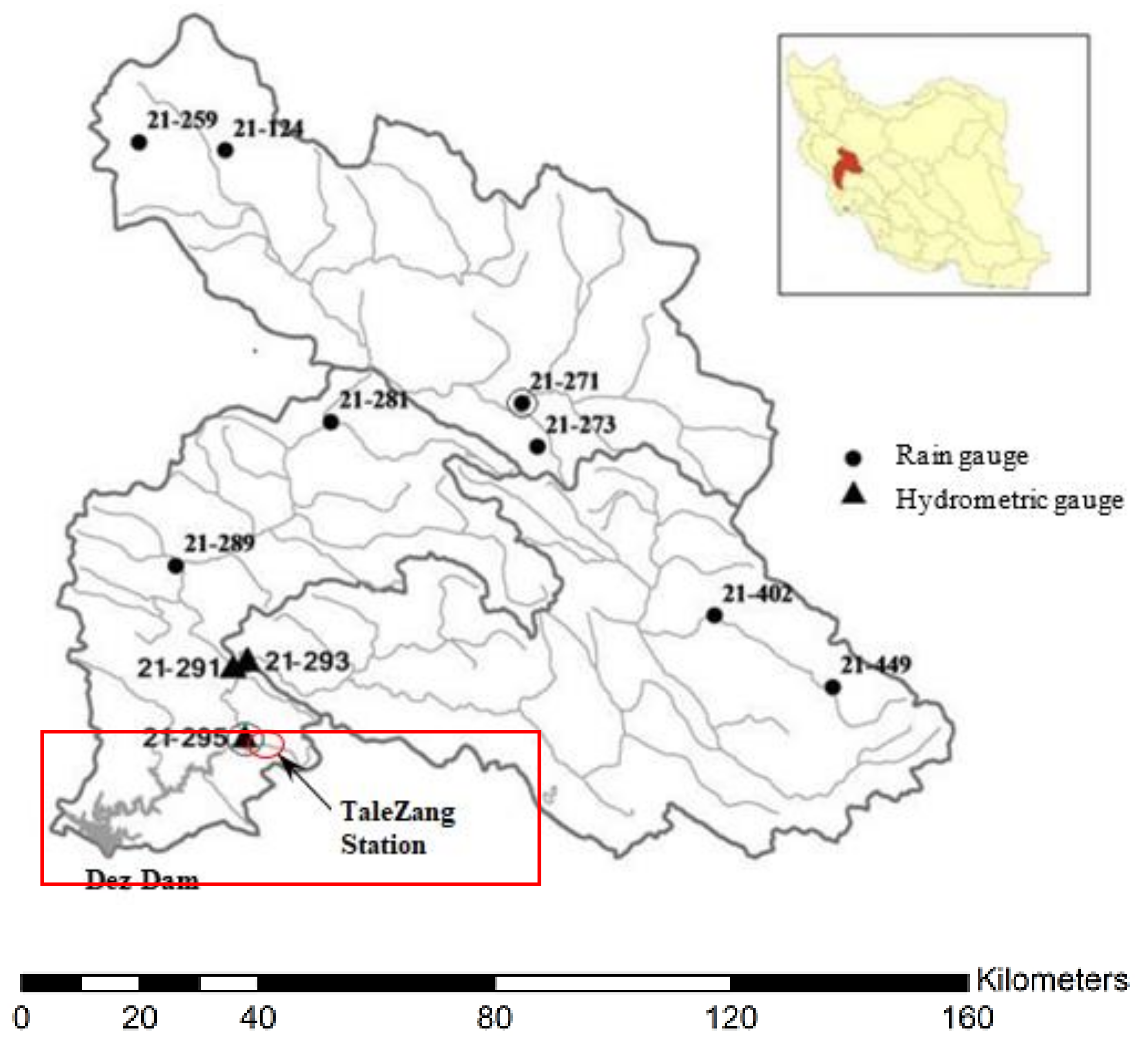
The second area chosen is Dez Basin, which has a considerably larger area and flow discharges than the former basin. This basin with an area of 23,252 km2 is located in the western part of Iran, between longitude 48°10′ to 50°20′ and latitude 31°36′ to 34°08′. The main river of the basin, Dez River, stems from the mountainous areas upstream, and ends up in the Persian Gulf. Half of the precipitation occurs during the winter. Two-thirds of the area is higher than 1000 m, and one-third is higher than 2000 m. Hence, precipitation most often occurs in the form of snow. Figure 5 shows the state of the Dez Dam and the monitoring stations spread throughout the basin. The monthly flow data from the TaleZang hydrometric station, upstream of Dez Dam, for 1962 to 1999 are available, and thus, only this period of data was used for predicting the monthly flows in this case study.
4. Results and Discussion
To employ the GPR for monthly flow prediction, a rational quadratic function was chosen as the appropriate kernel function and the basis function was considered as constant. The related parameters for the rational quadratic kernel were acquired as , , and . To use the SVR for prediction, the SVR algorithm was coded in MATLAB, and a GOA algorithm was then utilized to identify the best values for the SVR parameters. Table 1 shows the suitable parameter values of the GOA algorithm.
Support vector regression with quadratic kernel function was considered for prediction process. The optimal parameters for the quadratic kernel were obtained as and .
For the training of neural networks, as mentioned, the observed data were divided into three subsets: Training, validation, and test datasets. The previous verification data (from December 1996 to June 2001) used for the evaluation of the SVR are considered the test data of the ANNs. A portion of the remaining data (20%) is randomly selected as the validation dataset, and the other portion is used for training the networks (tuning the weights and biases). In order to avoid overfitting, K-fold cross-validation with k = 5 is used in all methods.
To select a suitable architecture, different architectures are checked; however, when considering different architectures, the arrangement of the training, validation, and testing data are not changed. Furthermore, the training of all architectures is started with the same initial weights and biases. The candidate architecture is constructed by only one hidden layer, and the network is allowed to incrementally increase the numbers of its neurons within a suitable range. This range depends on the amount of data available for training, and five to 20 neurons are considered herein. After stopping the training process, errors in the network, including (training + validation) the dataset and test dataset (also referred to as verification data), are checked and the network with the minimum level of error is chosen for a time series prediction.
For both the FFNN and TDNN, the best architecture was obtained as a network with 14 neurons in the hidden layer. For the RBFNN, the number of neurons was equal to the number of experimental pairs of training data, and the Gaussian function parameter was determined by the user through trial and error. Moreover, for the RNN, the best network contains 9 hidden neurons.
To compare the performance of the described techniques for a monthly flow prediction, several statistical metrics, including R, MRAE, MAE, AME, MSE, RMSE, and E, were considered. These metrics and their values are tabulated in Table 2 and Table 3 for the training and verification datasets, respectively. All metrics have an ideal value equal to zero except for R and E metrics, whose ideal value is 1.
In the first case study, the KNN model has the best performance according to the residual criteria for the results of verification data, including R, MSE, RMSE and E. Among the neural network models, RNN model has the highest correlation coefficient and the other predictors, i.e., FFNN, TDNN, and RFBNNs, showed almost the same level of performance in this case and SVR-Quadratic with optimal parameters, could not improve the prediction accuracy. In the models, such as ANNs, SVR, and GPR where there is a training step, as the number of noisy input variables increases, the prediction accuracy decreases. The KNN model, unlike other techniques, has no training process.
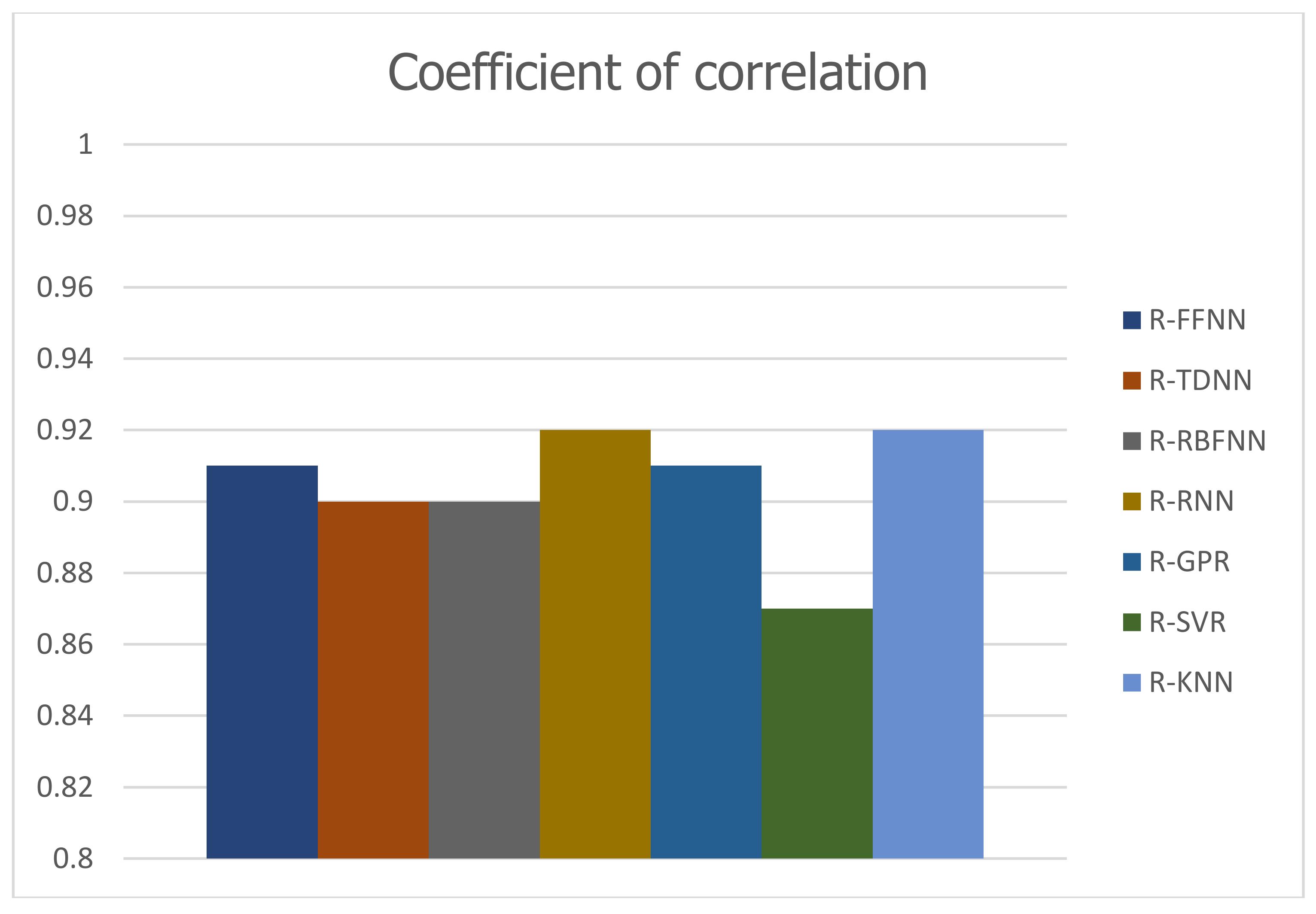
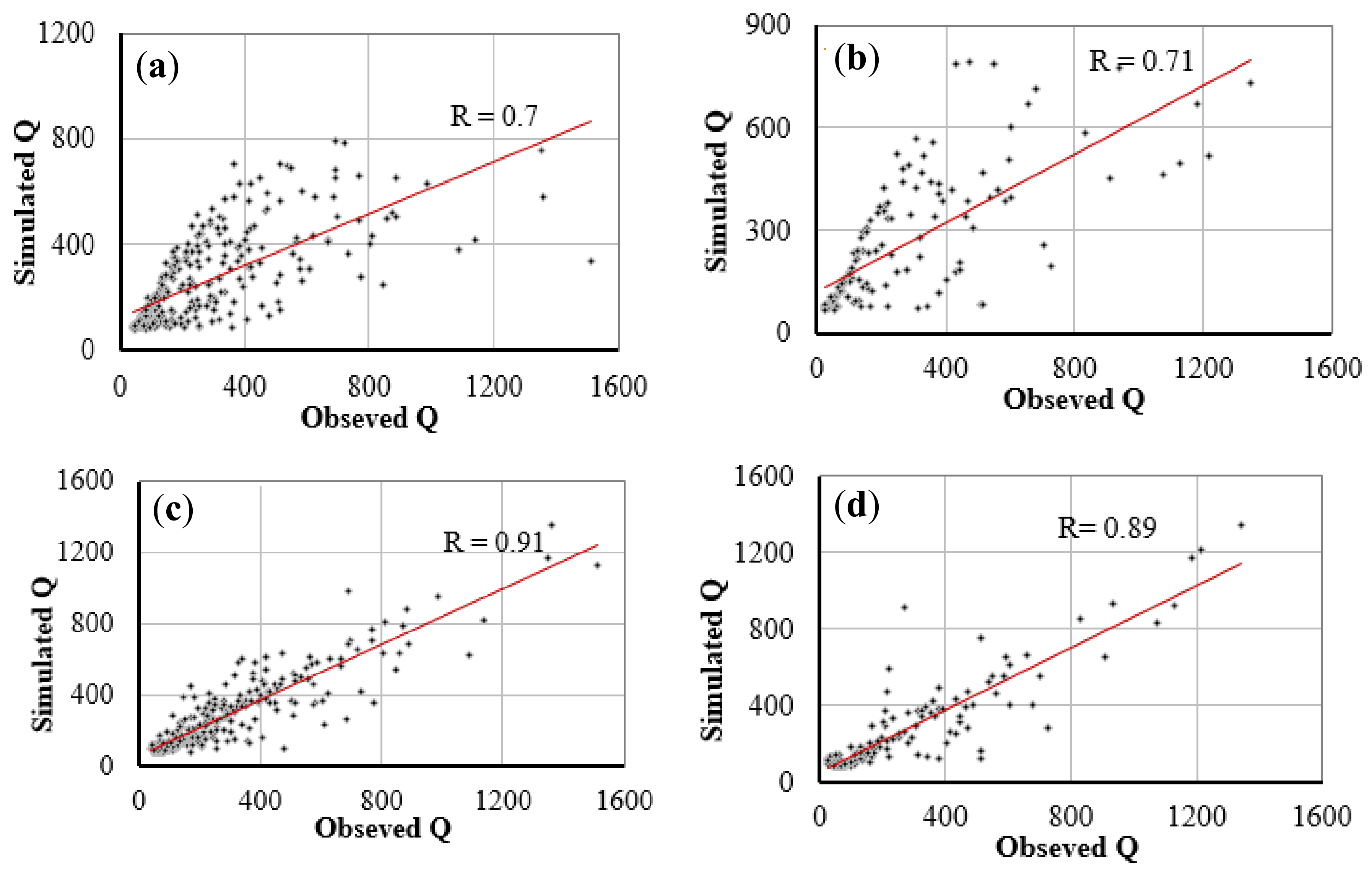
Figure 6 shows scatter plots of the observed discharges versus the predicted discharges during the training (left) and verification (right) periods for the five prediction models. This figure also confirms the KNN forecasting method has the desired performance based on the value of the correlation coefficient. In order to provide a visual comparison between the applied models, the results of the correlation coefficient (R), the most important criterion in the process of choosing the best model, are reported in the form of a bar histogram in Figure 7.
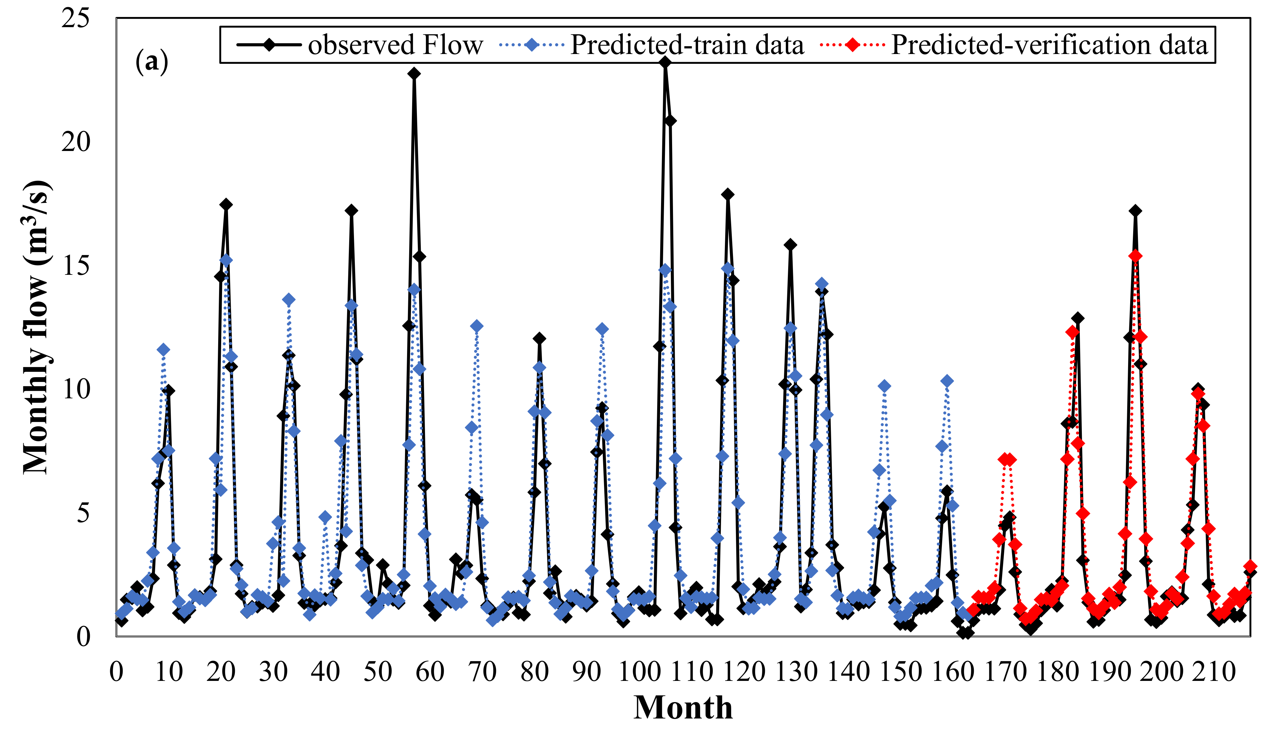
Figure 8 compares the flows predicted by the models with the flows observed during the verification periods. It can be seen that the RNN and RBFNN models produce mostly the same results, whereas the TDNN model has slightly worse prediction for low flows. Again, the KNN model shows highly accurate predictions, whereas less accurate results are obtained by the SVR with quadratic kernel.
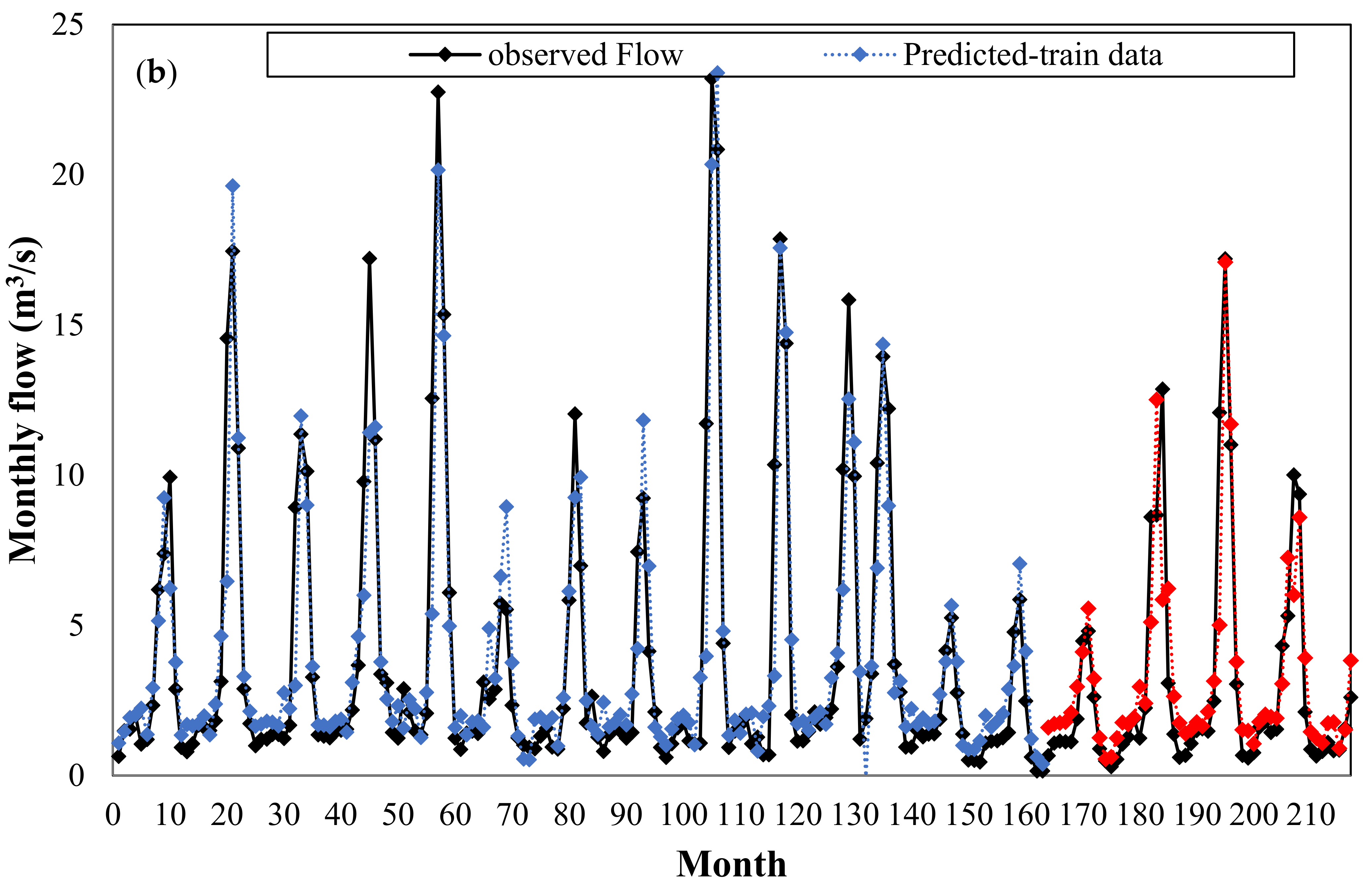
Figure 9 plots the observed and predicted flows by KNN model versus the whole time series period for June 1983 to June 2001 (during both the training and verification periods). This figure clearly demonstrates the high capability of the KNN model for predicting a monthly discharge.
The second case study was conducted on the Dez River Basin, which has considerably higher flow regimes and longer periods of observed data than the previous area. For this case, the only type of data available was on the monthly discharge, and thus monthly discharges with three temporal lags, i.e., Q(t − 2), Q(t − 1), and Q(t), were used as the input variables to predict the next month’s river discharge, Q(t + 1), as the output variable. In this case, the dataset from April 1962 to August 1988 (70% of the data) was selected for training, whereas the dataset from September 1988 to November 1999 (the remaining 30%) was used for verification.
To apply the GPR for monthly discharge prediction, the model with a squared exponential kernel function and a constant basis function was selected as the proper regression model. The related parameters for the rational quadratic kernel were acquired as and .
The optimal parameters for the SVR with a quadratic kernel were obtained as and . The best architecture for the FFNN, TDNN, and RNN models was obtained for networks with 14, 10, and 37 neurons in the hidden layer, respectively.
The results of training and verification based on residual metrics are shown in Table 4 and Table 5, respectively. Here, the best performance is by the RBFNN model based on R, AME, MSE, RMSE and E criteria. The RBFNN model showed the better performance because in this case study there were more observed data, and RBF networks perform better than other NNs as there is a large number of training vectors available [30].
Comparing other neural network models, it is evident that RBFNN has the best performance according to the and E criteria. Furthermore, the results of R, MSE, RMSE and E criteria from these two case studies also show that the FFNN outperforms the TDNN. This means that establishing a static neural network (or FFNN) with independent input variables of the time lags is more successful for time series prediction than time delay network configurations, which have a smaller number of input variables, but with delay signals.
Figure 10 shows the scatter plots of observed discharges versus the predicted discharges during the training (left) and verification periods (right), and the correlation coefficient for the best and the worst prediction models. The RBFNN method is also more accurate in terms of the correlation coefficient. As displayed in Figure 11, the bar histogram of correlation coefficient values acquired from various models shows the best performance of NNRBF model.
Figure 12 shows a graphical comparison of the observed data and the results of the prediction models for the verification period in Dez Basin. The FFNN and TDNN models show a relatively suitable prediction for median and low flows, but their prediction capability for extreme flows is poor. The RBFNN model predicts extreme flows slightly better than the two previous models. Although the GPR, SVR-Quadratic, and KNN models have the relatively same prediction quality, their prediction performance is weaker than the RBFNN, FFNN, and RNN models. Figure 13 shows the observed and predicted discharges of the RBFNN model for the whole time series, from April 1962 to November 1999.
5. Conclusions
In this study, GPR and GOA based SVR models were applied to predict long-term river flows in Alavian and Dez Basins based on historical records. Five other machine learning algorithms, i.e., feedforward neural network, time delay neural network, radial basis neural network, recurrent neural network, and KNN were also established to verify the capability of these algorithms for discharge prediction. Through a comparison of the results based on the value of the coefficient of correlation, it was found that the KNN model, without any training process in which a part of noisy data is used to train the model, and RBFNN model can provide more accurate predictions for Alavian and Dez Basins, respectively. In the first study area, Alavian Basin, where there were six predictor variables, the KNN and RNN models have the maximum correlation coefficient in comparison to other models. Based on MRAE criterion for the verification data, the FFNN model is the most accurate prediction model and the GPR has a better performance than the SVR-Quadratic and KNN models. In the first study area, KNN has the lowest prediction error in terms of MAE and MSE criteria. In addition, FFNN with a lower value of MAE and MSE criteria than TDNN, RBFNN, RNN, GPR, and SVR-Quadratic, provides more accurate predictions. Also, the RNN model has less predictive accuracy in terms of MRAE, MAE, and RMSE than FFNN and RBFNN models in Alavian Basin. In the second case study, Dez Basin with more observations, but fewer features, in comparison to the first study area, the RBFNN model has been selected as the best predictor model based on correlation coefficient (R) criterion for the verification data. Although, the SVR model linked with a powerful optimizer, i.e., the GOA algorithm to identify the SVR parameters, leads to more accurate predictions than the GPR and KNN models in terms of R criterion, but it was not precise enough for extreme point predictions and based on MAE criterion, it has undesirable performance in comparison to other prediction models. In the study area according to MAE, AME and MSE criteria, RBFNN has more accurate predictions than FFNN, TDNN, RNN, GPR, SVR-Quadratic, and KNN. Furthermore, the RNN model has a higher prediction error in terms of MRAE, MAE, AME, and MSE in comparison to FFNN and RBFNN models in Dez Basin. Considering AME, and RMSE, the GPR model has a more accurate prediction than the SVR-Quadratic and KNN models.
As a result, comparing the results of the current study, developing a GOA-SVR model, with many of previous ones indicated that the GPR and SVR models are not always the best estimators in time series prediction.
Applying other optimization algorithms, suggested for future researches, can affect the model efficiency. Furthermore, changing the time step of observations (e.g., using daily data instead of monthly ones) is proposed as another suggestion for future studies that may vary the derived results from various models.
Supplementary Materials
Supplementary File 1Author Contributions
Methodology, Zahra Alizadeh, Jafar Yazdi and Abobakr Khalil Al-Shamiri; formal analysis, Zahra Alizadeh and Jafar Yazdi; funding acquisition, Joong Hoon Kim.
Funding
This research was supported by the National Research Foundation of Korea (NRF) grant funded by the Korean government (MSIP) (No. 2016R1A2A1A05005306).
Conflicts of Interest
The authors declare no conflicts of interest.
References
- Box, G.E.; Jenkins, G.M.; Reinsel, G.C. Time Series Analysis: Forecasting and Control, 4th ed.; John Wiley & Sons Inc.: Hoboken, NJ, USA, 2013; ISBN 978-1-118-61919-3. [Google Scholar]
- Tokar, A.S.; Johnson, P.A. Rainfall-runoff modeling using artificial neural networks. J. Hydrol. Eng. 1999, 4, 232–239. [Google Scholar] [CrossRef]
- Khashei, M.; Bijari, M. A novel hybridization of artificial neural networks and ARIMA models for time series forecasting. Appl. Soft Comput. 2011, 11, 2664–2675. [Google Scholar] [CrossRef]
- Feng, L.H.; Lu, J. The practical research on flood forecasting based on artificial neural networks. Expert Syst. Appl. 2010, 37, 2974–2977. [Google Scholar] [CrossRef]
- Pumo, D.; Francipane, A.; Lo Conti, F.; Arnone, E.; Bitonto, P.; Viola, F.; La Loggia, G.; Noto, L.V. The SESAMO early warning system for rainfall-triggered landslides. J. Hydroinform. 2016, 18, 256–276. [Google Scholar] [CrossRef] [Green Version]
- Zounemat-Kermani, M.; Kisi, O.; Rajaee, T. Performance of radial basis and lm-feed forward artificial neural networks for predicting daily watershed runoff. Appl. Soft Comput. 2013, 13, 4633–4644. [Google Scholar] [CrossRef]
- Giustolisi, O.; Laucelli, D. Improving generalization of artificial neural networks in rainfall–runoff modelling. Hydrol. Sci. J. 2005, 50, 439–457. [Google Scholar] [CrossRef]
- Yu, J.; Qin, X.; Larsen, O.; Chua, L. Comparison between response surface models and artificial neural networks in hydrologic forecasting. J. Hydrol. Eng. 2013, 19, 473–481. [Google Scholar] [CrossRef]
- Thissen, U.; Van Brakel, R.; De Weijer, A.; Melssen, W.; Buydens, L. Using support vector machines for time series prediction. Chemom. Intell. Lab. Syst. 2003, 69, 35–49. [Google Scholar] [CrossRef]
- Chiu, D.Y.; Chen, P.J. Dynamically exploring internal mechanism of stock market by fuzzy-based support vector machines with high dimension input space and genetic algorithm. Expert Syst. Appl. 2009, 36, 1240–1248. [Google Scholar] [CrossRef]
- Malekmohamadi, I.; Bazargan-Lari, M.R.; Kerachian, R.; Nikoo, M.R.; Fallahnia, M. Evaluating the efficacy of svms, bns, anns and anfis in wave height prediction. Ocean Eng. 2011, 38, 487–497. [Google Scholar] [CrossRef]
- Karamouz, M.; Ahmadi, A.; Moridi, A. Probabilistic reservoir operation using Bayesian stochastic model and support vector machine. Adv. Water Resour. 2009, 32, 1588–1600. [Google Scholar] [CrossRef]
- Chiang, J.; Tsai, Y. Reservoir drought prediction simulation using support vector machines. Appl. Mech. Mater. 2011, 145, 455–459. [Google Scholar] [CrossRef]
- Çimen, M.; Kisi, O. Comparison of two different data-driven techniques in modeling lake level fluctuations in turkey. J. Hydrol. 2009, 378, 253–262. [Google Scholar] [CrossRef]
- Noori, R.; Karbassi, A.; Moghaddamnia, A.; Han, D.; Zokaei-Ashtiani, M.; Farokhnia, A.; Gousheh, M.G. Assessment of input variables determination on the SVM model performance using PCA, gamma test, and forward selection techniques for monthly stream flow prediction. J. Hydrol. 2011, 401, 177–189. [Google Scholar] [CrossRef]
- Kalteh, A.M. Wavelet Genetic Algorithm-Support Vector Regression (Wavelet GA-SVR) for Monthly Flow Forecasting. Water Resour. Manag. 2014, 29, 1283–1293. [Google Scholar] [CrossRef]
- Hosseini, S.M.; Mahjouri, N. Integrating Support Vector Regression and a geomorphologic Artificial Neural Network for daily rainfall-runoff modeling. Appl. Soft Comput. 2016, 38, 329–345. [Google Scholar] [CrossRef]
- Pumo, D.; Viola, F.; Noto, L.V. Generation of natural runoff monthly series at ungauged sites using a regional regressive model. Water 2016, 8, 209. [Google Scholar] [CrossRef] [Green Version]
- Saremi, S.; Mirjalili, S.; Lewis, A. Grasshopper Optimisation Algorithm: Theory and application. Adv. Eng. Softw. 2017, 105, 30–47. [Google Scholar] [CrossRef]
- Wu, C.L.; Chau, K.W. Data-driven models for monthly streamflow time series prediction. Eng. Appl. Artif. Intell. 2010, 23, 1350–1367. [Google Scholar] [CrossRef] [Green Version]
- Akbari, M.; Overloop, P.J.V.; Afashar, A. Clustered K Nearest Neighbor Algorithm for Daily Inflow Forecasting. Water Resour. Manag. 2011, 25, 1341–1357. [Google Scholar] [CrossRef]
- Rasmussen, C.E.; Williams, C.K.I. Gaussian Process for Machine Learning, Adaptive Computational and Machine Learning; MIT Press: Cambridge, MA, USA; London, UK, 2006; ISBN 026218253X. [Google Scholar]
- Schölkopf, B.; Smola, A.J. Learning with Kernels: Support Vector Machines, Regularization, Optimization, and Beyond; MIT Press: Cambridge, MA, USA; London, UK, 2002; ISBN 978-0262194754. [Google Scholar]
- Yazdi, J.; Hokmabadi, A.; Jalili-Ghazizadeh, M.R. Optimal Size and Placement of Water Hammer Protective Devices in Water Conveyance Pipelines. Water Resour. Manag. 2018. accepted. [Google Scholar] [CrossRef]
- Engelbrecht, A.P. Computational Intelligence: An Introduction, 2nd ed.; John Wiley & Sons: New York, NY, USA, 2007. [Google Scholar]
- Beale, M.; Hagan, M.; Demuth, H. Neural Network Toolbox User’s Guide; The MathWorks Inc.: Natick, MA, USA, 2010. [Google Scholar]
- Maier, H.R.; Jain, A.G.; Dandy, C.; Sudheer, K.P. Methods used for the development of neural networks for the prediction of water resource variables in river systems: Current status and future directions. Environ. Model. Softw. 2010, 25, 891–909. [Google Scholar] [CrossRef]
- Leshno, M.; Lin, V.Y.; Pinkus, A.; Schocken, S. Multilayer feedforward networks with a nonpolynomial activation function can approximate any function. Neural Netw. 1993, 6, 861–867. [Google Scholar] [CrossRef] [Green Version]
- Picton, P. Neural Networks, 2nd ed.; Palgrave Macmillan: New York, NY, USA, 2000. [Google Scholar]
- Araghinejad, S. Data-Driven Modeling: Using MATLAB® in Water Resources and Environmental Engineering; Springer: Berlin, Germany, 2014; ISBN 978-94-007-7506-0. [Google Scholar]
- Lang, K.J.; Waibel, A.H.; Hinton, G.E. A time-delay neural network architecture for isolated word recognition. Neural Netw. 1990, 3, 23–43. [Google Scholar] [CrossRef]
Figure 1.
A feedforward neural network (FFNN).

Figure 2.
A single time delay neuron.

Figure 3.
A recurrent neural network (RNN).

Figure 4.
Map of the Alavian River Basin.

Figure 5.
Map of the Dez River Basin.

Figure 6.
Performance of SVR-Quadratic and KNN (the worst and best techniques) in terms of correlation coefficient for Alavian Basin: (a) SVR-Quadratic_training data; (b) SVR-Quadratic_verification data; (c) KNN-training data; (d) KNN- verification data.
Figure 6.
Performance of SVR-Quadratic and KNN (the worst and best techniques) in terms of correlation coefficient for Alavian Basin: (a) SVR-Quadratic_training data; (b) SVR-Quadratic_verification data; (c) KNN-training data; (d) KNN- verification data.

Figure 7.
Bar histogram of the correlation coefficient (R) values derived from various models.

Figure 8.
Monthly flow prediction for verification dataset for Alavian Basin: (a) NNRBF and RNN, and (b) NNRBF, SVR-Quadratic, KNN, and GPR.
Figure 8.
Monthly flow prediction for verification dataset for Alavian Basin: (a) NNRBF and RNN, and (b) NNRBF, SVR-Quadratic, KNN, and GPR.

Figure 9.
Comparing the observed flows with the predicted flows obtained by (a) KNN and (b) SVR-Quadratic for the period 1983–2001 for Alavian Basin.
Figure 9.
Comparing the observed flows with the predicted flows obtained by (a) KNN and (b) SVR-Quadratic for the period 1983–2001 for Alavian Basin.


Figure 10.
Performance of TDNN and NNRBF (the worst and best techniques) in terms of correlation coefficient for Dez Basin. (a) TDNN- training data; (b) TDNN- verification data; (c) NNRBF- training data; (d) NNRBF- verification data.
Figure 10.
Performance of TDNN and NNRBF (the worst and best techniques) in terms of correlation coefficient for Dez Basin. (a) TDNN- training data; (b) TDNN- verification data; (c) NNRBF- training data; (d) NNRBF- verification data.

Figure 11.
Bar histogram of the correlation coefficient (R) values obtained from various models.

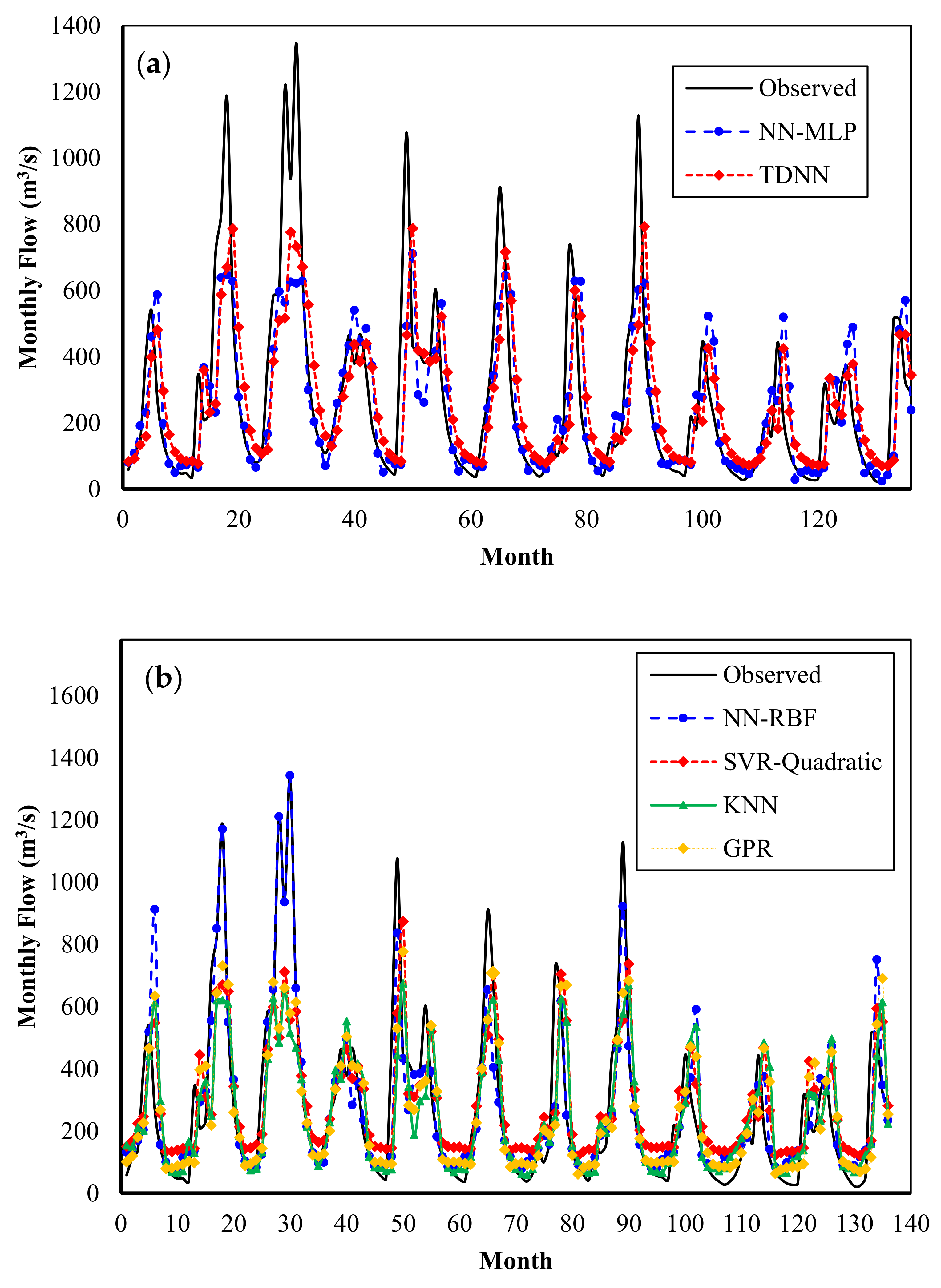
Figure 12.
Monthly flow prediction for verification dataset for Dez Basin: (a) NN-MLP and TDNN, and (b) NNRBF, SVR-Quadratic, KNN and GPR.
Figure 12.
Monthly flow prediction for verification dataset for Dez Basin: (a) NN-MLP and TDNN, and (b) NNRBF, SVR-Quadratic, KNN and GPR.

Figure 13.
Comparison of the observed flows with predicted flows obtained by (a) NN-RBF and (b) TDNN for the period 1962–1999 for Dez Basin.
Figure 13.
Comparison of the observed flows with predicted flows obtained by (a) NN-RBF and (b) TDNN for the period 1962–1999 for Dez Basin.


Table 1.
The parameters used in the grasshopper optimization algorithm (GOA).
| Parameter | Lower Bound | Upper Bound | Search Agents | Max Iteration |
|---|---|---|---|---|
| 0.01 | 0.3 | 100 | 100 | |
| 1 | 100 |
Table 2.
Residual criteria for the results of training data for Alavian Basin, where n is the number of observations, yi and are the simulated and observed data, respectively, and is the average observed data.
Table 2.
Residual criteria for the results of training data for Alavian Basin, where n is the number of observations, yi and are the simulated and observed data, respectively, and is the average observed data.
| Criteria | Formula | FFNN | TDNN | RBFNN | RNN | GPR | SVR-Quadratic | KNN |
|---|---|---|---|---|---|---|---|---|
| correlation coefficient (R) | 0.94 | 0.95 | 0.93 | 0.92 | 0.94 | 0.92 | 0.88 | |
| Mean Relative Absolute Error (MRAE) | 0.378 | 0.425 | 0.464 | 0.53 | 0.43 | 0.45 | 0.47 | |
| Mean Absolute Error (MAE) | 1.051 | 0.947 | 1.181 | 1.25 | 1.23 | 1.13 | 1.41 | |
| Absolute Maximum Error (AME) | 6.492 | 6.250 | 7.2511 | 8.44 | 7.16 | 8.08 | 8.73 | |
| Mean Square Error (MSE) | 2.627 | 2.046 | 3.213 | 3.99 | 4.02 | 3.35 | 5.35 | |
| Root Mean Square Error (RMSE) | 1.621 | 1.430 | 1.792 | 1.99 | 2.01 | 1.83 | 2.31 | |
| Nash-Sutcliffe Coefficient (E) | 0.885 | 0.910 | 0.859 | 0.83 | 0.81 | 0.85 | 0.77 |
Table 3.
Residual criteria for the results of verification data, Alavian Basin.
| Criteria | FFNN | TDNN | RBFNN | RNN | GPR | SVR-Quadratic | KNN |
|---|---|---|---|---|---|---|---|
| R | 0.91 | 0.9 | 0.9 | 0.92 | 0.91 | 0.87 | 0.92 |
| MRAE | 0.491 | 0.670 | 0.513 | 0.7 | 0.5 | 0.55 | 0.53 |
| MAE | 0.977 | 1.048 | 1.041 | 1.13 | 0.99 | 1.11 | 0.95 |
| AME | 5.936 | 5.804 | 5.753 | 5.78 | 6.16 | 7.07 | 5.84 |
| MSE | 2.451 | 2.710 | 2.772 | 2.79 | 2.6 | 3.39 | 2.23 |
| RMSE | 1.566 | 1.646 | 1.665 | 1.67 | 1.61 | 1.84 | 1.49 |
| E | 0.822 | 0.803 | 0.7985 | 0.81 | 0.81 | 0.76 | 0.84 |
Table 4.
Residual criteria for the results of the data training for Dez Basin.
| Criteria | FFNN | TDNN | RBFNN | RNN | GPR | SVR-Quadratic | KNN |
|---|---|---|---|---|---|---|---|
| R | 0.76 | 0.7 | 0.91 | 0.7 | 0.77 | 0.74 | 0.71 |
| MRAE | 0.365 | 0.538 | 0.292 | 0.55 | 0.42 | 0.67 | 0.36 |
| MAE | 96.815 | 125.487 | 62.5402 | 113.64 | 94.169 | 112.2 | 94.79 |
| AME | 1092.976 | 1177.905 | 418.0132 | 1210.2 | 1095.94 | 1178.4 | 1132.9 |
| MSE | 27,871.642 | 36,228.586 | 10,857.818 | 29,642.51 | 23,597.1 | 26,823.89 | 28,282 |
| RMSE | 166.948 | 190.338 | 104.201 | 172.17 | 153.61 | 163.78 | 168.17 |
| E | 0.553 | 0.414 | 0.826 | 0.48 | 0.59 | 0.53 | 0.5 |
Table 5.
Residual criteria for the results of verification data for Dez Basin.
| Criteria | FFNN | TDNN | RBFNN | RNN | GPR | SVR-Quadratic | KNN |
|---|---|---|---|---|---|---|---|
| R | 0.75 | 0.71 | 0.89 | 0.82 | 0.73 | 0.73 | 0.72 |
| MRAE | 0.503 | 9.508 | 0.807 | 0.65 | 0.58 | 0.67 | 0.55 |
| MAE | 92.649 | 103.872 | 78.786 | 111.55 | 118.2 | 131.51 | 117.15 |
| AME | 526.256 | 632.494 | 373.554 | 581.38 | 764.72 | 785.74 | 826.99 |
| MSE | 20,467.509 | 23,024.515 | 12,757.705 | 24,670.98 | 34,144.9 | 34,384.28 | 35,878.1 |
| RMSE | 143.065 | 155.391 | 112.950 | 157.07 | 184.78 | 185.43 | 189.42 |
| E | 0.536 | 0.447 | 0.711 | 0.67 | 0.53 | 0.53 | 0.51 |
© 2018 by the authors. Licensee MDPI, Basel, Switzerland. This article is an open access article distributed under the terms and conditions of the Creative Commons Attribution (CC BY) license (http://creativecommons.org/licenses/by/4.0/).
Share and Cite
MDPI and ACS Style
Alizadeh, Z.; Yazdi, J.; Kim, J.H.; Al-Shamiri, A.K. Assessment of Machine Learning Techniques for Monthly Flow Prediction. Water 2018, 10, 1676. https://doi.org/10.3390/w10111676
AMA Style
Alizadeh Z, Yazdi J, Kim JH, Al-Shamiri AK. Assessment of Machine Learning Techniques for Monthly Flow Prediction. Water. 2018; 10(11):1676. https://doi.org/10.3390/w10111676
Chicago/Turabian StyleAlizadeh, Zahra, Jafar Yazdi, Joong Hoon Kim, and Abobakr Khalil Al-Shamiri. 2018. "Assessment of Machine Learning Techniques for Monthly Flow Prediction" Water 10, no. 11: 1676. https://doi.org/10.3390/w10111676
Note that from the first issue of 2016, this journal uses article numbers instead of page numbers. See further details here.