Monthly Rainfall-Runoff Modeling at Watershed Scale: A Comparative Study of Data-Driven and Theory-Driven Approaches

1
Department of Mathematical Sciences, College of Arts and Sciences, University of Cincinnati, 2825 Campus Way, Cincinnati, OH 45221, USA
2
Department of Geography and Geographic Information Science, College of Arts and Sciences, University of Cincinnati, 2825 Campus Way, Cincinnati, OH 45221, USA
*
Author to whom correspondence should be addressed.
Water 2018, 10(9), 1116; https://doi.org/10.3390/w10091116
Submission received: 27 July 2018
/
Revised: 19 August 2018
/
Accepted: 20 August 2018
/
Published: 22 August 2018
(This article belongs to the Section Hydrology)
Abstract
:Data-driven machine learning approaches have been rapidly developed in the past 10 to 20 years and applied to various problems in the field of hydrology. To investigate the capability of data-driven approaches in rainfall-runoff modeling in comparison to theory-driven models, we conducted a comparative study of simulated monthly surface runoff at 203 watersheds across the contiguous USA using a conceptual model, the proportionality hydrologic model, and a data-driven Gaussian process regression model. With the same input variables of precipitation and mean monthly aridity index, the two models showed similar performance. We then introduced two more input variables in the data-driven model: potential evaporation and the normalized difference vegetation index (NDVI), which were selected based on hydrologic knowledge. The modified data-driven model performed much better than either the conceptual or original data-driven model. A sensitivity analysis was conducted on all three models tested in this study, which showed that surface runoff responded positively to increased precipitation. However, a confounding effect on surface runoff sensitivity was found among mean monthly aridity index, potential evaporation, and NDVI. This confounding was caused by complex interconnections among energy supply, vegetation coverage, and climate seasonality of the watershed system. We also conducted an uncertainty analysis on the two data-driven models, which showed that both models had reasonable predictability within the 95% confidence interval. With the additional two input variables, the modified data-driven model had lower prediction uncertainty and higher prediction accuracy.
1. Introduction
With the rapid development of computational capability, data-driven machine learning methods have become more popular in the past decade in all fields related to data and modeling, including hydrology (e.g., [1,2,3,4,5,6,7]). Unlike typical hydrologic models, data-driven approaches do not rely directly on explicit physical knowledge of the target process. Instead, they build a purely empirical model based on observed relationships between input and output variables. Using various learning algorithms (e.g., [8,9,10,11,12]), data-driven approaches provide a flexible way to model complex phenomena such as runoff generation. State-of-the-art algorithms such as artificial neural network [1,4] and Gaussian process regression [13] have been applied to hydrologic modeling. For example, Sun et al. [13] built a data-driven model based on the Gaussian process regression algorithm to predict monthly streamflow at over 400 watersheds in the US and showed generally good performance of the model. Elshorbagy et al. [5,6] compared the capabilities of six data-driven approaches in modeling various hydrologic variables, such as evapotranspiration, soil moisture content, and runoff. A data-driven approach is especially useful when (1) the current human knowledge of the process is not enough to provide an explicit modeling strategy [14] or (2) physical modeling is too challenging due to complexity of the target process [15].
Furthermore, data-driven approaches can also be linked with knowledge of physical principles and therefore physical plausibility [16,17,18]. Kingston et al. [19] presented a calibration and validation approach to show the connection between the knowledge of a physical system provided in the input data and the physical plausibility of a data-driven model. Mount et al. [20] used partial derivative input sensitivity analysis to evaluate the physical legitimacy of data-driven models. The connection between data-driven models and physical plausibility indicates that there is great potential to use data-driven models to discover new system dynamics and identify new physical mechanisms [14].
Compared to data-driven methods, most conventional hydrologic models can be considered to be theory-driven. Many comparison studies have been conducted to show the advantages and disadvantages of theory-driven models and data-driven models. Anctil et al. [21] showed that artificial neural network can achieve similar performance as a conceptual hydrologic model on streamflow simulation. They also found that a longer period of observation records was more beneficial to the neural network approach than to the conceptual model. Toth and Brath [22] compared the real-time streamflow forecasting capability of a conceptual model and an artificial neural network approach and found that the neural network approach performed well with continuous streamflow and precipitation data, while the conceptual model was preferable when data were limited. In these comparison studies, the level of model structure complexity of the data-driven model, in terms of number of parameters and equations, was much higher than the counterpart conceptual model. Comparing a data-driven model and a theory-driven model with similar levels of model complexity may help us gain better understanding of both types of models.
Guided by insights from previous studies, in this paper we conduct a systematic comparative study on theory-driven and data-driven models of simulated monthly rainfall-runoff at 203 watersheds across the contiguous US. Rainfall-runoff relationships have been studied extensively within the field of hydrology. However, hydrologic systems at an intra-annual temporal scale, including seasonally and monthly, show some unique characteristics that have not been fully understood and modeled [23,24,25]. We aim to investigate whether data-driven methods with similar levels of input information and numbers of model parameters can provide modeling performance comparable to theory-driven models and also represent physical mechanisms in surface runoff generation at a monthly time scale in watersheds in different climate regions across the contiguous US. This requires a modelling framework that can consistently maintain high transparency, flexibility, and physical plausibility in a wide range of geographical settings without elaborate area-specific modifications. (This requirement is quite different from that for more area-specific studies, as they require highly customized modeling schemes of particular regions.) We therefore employed a Gaussian process regression (GPR) model, which allows flexible modeling of surface runoff in an automated fashion. As for the counterpart theory-driven model, we selected the proportionality hydrologic model (PHM), which also has a simple model structure and has shown satisfactory performance in the study region [26]. It should be noted that we are focusing on surface runoff generation modeling in this study, not total runoff. Surface runoff generation and baseflow generation are two different physical processes, and their controlling factors are not the same. Therefore, we focus on surface runoff generation as an individual physical process that is part of total runoff generation. Baseflow generation modeling will be our next study objective, which is beyond the scope of this study.
To be more specific, we started with a comparative study between the theory-driven PHM and data-driven GPR given the same input variables. Then we prepared additional input data for GPR based on hydrologic knowledge and expert judgment to improve its performance, and therefore to assess the effectiveness of incorporating hydrologic knowledge in our data-driven modeling framework. Next, we conducted a sensitivity analysis on all three models to show the controlling effect of input variables on monthly surface runoff and investigate the physical plausibility of the models. Finally, we conducted an uncertainty analysis on the two data-driven models to evaluate their prediction coverage within a 95% confidence interval.
2. Study Watersheds and Data Sources
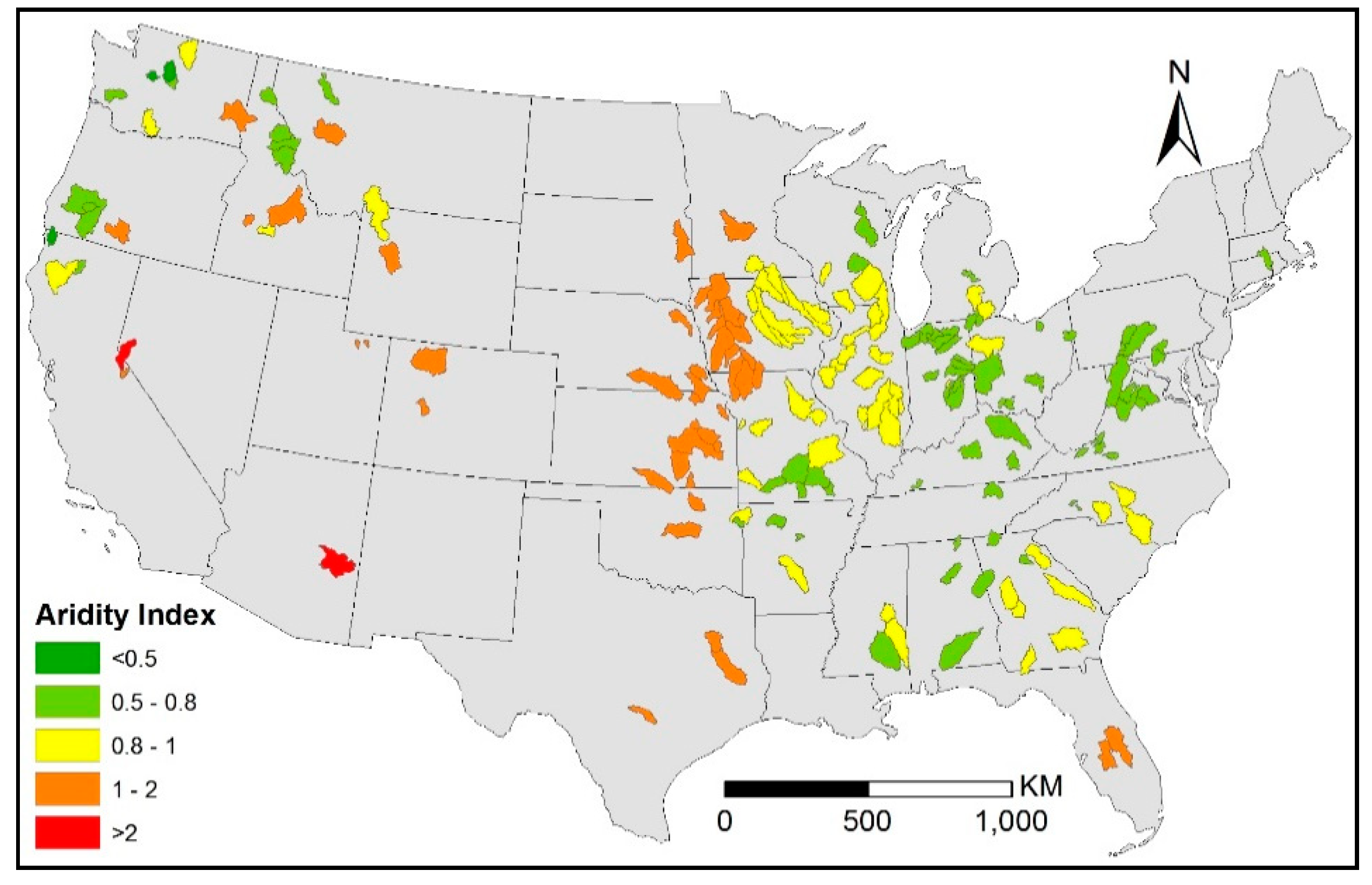
Hydrometeorological data from the Model Parameter Estimation Experiment (MOPEX) were used in this study [27]. From a total of 438 MOPEX watersheds across the contiguous US, we selected 203 with higher data accuracy [25,26] (Figure 1). For the study watersheds, we collected daily precipitation and streamflow data from 1983 to 2002 from MOPEX. The streamflow data were separated into surface runoff and baseflow using the one-parameter digital filter method with a filter parameter value of 0.925 [28]. The surface runoff data from the separation were used in this study. The monthly potential evaporation data from 1983 to 2002 were collected from Zhang et al. [29] and validated with flux tower measurements. Values of mean monthly aridity index were obtained from Chen et al. [25] to determine seasonality of the study watersheds. Finally, we used the normalized difference vegetation index (NDVI) to represent vegetation coverage. Bimonthly NDVI data were collected from Advanced Very High Resolution Radiometer (AVHRR) imagery from the Global Inventory Modeling and Mapping Studies (GIMMS), which can be downloaded at http://staff.glcf.umd.edu/sns/htdocs/data/gimms/index.shtml [30]. All the different types of data collected in this study were converted to watershed scale with monthly time steps.
3. Methodology
3.1. Theory-Driven Conceptual Hydrologic Model
The theory-driven model we selected in this study is the proportionality hydrologic model (PHM), a simple conceptual hydrologic model with 2 equations for the surface runoff simulation [26]:
where Qd is surface runoff (mm), P is precipitation (mm), λ is initial wetting fraction, and W is wetting capacity (mm). In this model, is the only monthly input, while and are parameters with fixed values for each watershed. In addition, as part of model input preparation, we divided monthly data into energy-limited months with subscript e and water-limited months with subscript w, based on the mean monthly aridity index [25]:
where is the mean monthly aridity index of month , is the mean monthly potential evaporation (mm), is the mean monthly precipitation (mm), and is the mean monthly water storage change (mm). The values of for the 203 study watersheds were obtained from Chen et al. [25]. Energy-limited months are the ones with ≤ 1 and water-limited months are the ones with > 1. Surface runoff in energy-limited months was modeled using Equation (1) and in water-limited months by Equation (2). The equations are similar, but with 2 different sets of and . All the energy-limited months in a year form the energy-limited season and the water-limited months in a year form the water-limited season. This model is based on the proportionality hypothesis [31], which is derived from the Soil Conservation Service (SCS) curve number method [32]. This model has shown capability to simulate surface runoff and streamflow in various watersheds at an intra-annual scale [26,33].
In PHM, monthly precipitation is the only monthly input. The mean monthly aridity index is used to define the seasonality of each month, which can be considered as indirect input. For the PHM simulation, the parameter values of λe, λw, We, and Ww were calibrated using the data from 1983 to 1992. The calibration was done by simulating surface runoff using all possible combinations of parameter values within predefined parameter value ranges [26] and selecting the combination with the highest Nash–Sutcliffe efficiency (NSE) value. The calibrated PHM was then used to simulate monthly surface runoff using precipitation as input in the period 1993 to 2002 for model validation.
3.2. Data-Driven Method
The data-driven approach that we employed in this study is the Gaussian process regression model (e.g., [9,34]), which has been widely used in various areas including hydrology (e.g., [13]), climate science (e.g., [35,36,37]), and glaciology (e.g., [38,39,40,41,42]). This data-driven approach can generate a flexible functional relationship between the predictor and response variables. The Gaussian process regression model has some mathematical connection to other methods, such as neural network [9,43] and spline regression [44], therefore it often yields similar results to these approaches.
The main reason that we chose the Gaussian process regression model is its parsimonious structure compared to other popular approaches such as artificial neural network (ANN) (e.g., [45]). Our GPR has a similar level of complexity to the conceptual PHM. Both models have 2 main equations. PHM has 4 parameters and GPR has 7. Another reason is that the Gaussian process model can provide a competitive solution in a highly automated manner. In fact, the method requires specification of only the covariance structure, for which the Matérn covariance function can be used in most cases [34]. Due to this advantage, we can model various types of complex relationships between the target response variable (i.e., monthly runoff) and the input variables for a large number of watersheds with high flexibility. Moreover, due to its parsimonious structure, GPR often does not suffer from overfitting issues, unlike more parameterized methods such as ANN.
We trained the following Gaussian process model to learn about the relationship between the input variables , which are also called predictors () in data-driven methods, and the surface runoff Qd:
where and are surface runoff and predictors at time point ; θ is the power for variable transformation; and are intercept and regression coefficients; is a Gaussian process with the covariance function defined in Equation (5); is an indicator function with a value of 1 if the condition in holds and 0 otherwise; the parameters , , >0 are covariance parameters to be estimated as part of model training; and the correlation function K is a prespecified correlation function. In this study, we used a Matérn correlation function with smoothness parameter 1.5, but the result is not sensitive to the choice of smoothness parameter. The coefficients and the covariance parameters and are estimated using maximum restricted likelihood estimation (see Stein [34], Section 6.4 for details), meaning that the objective function we used in model fitting is the restricted likelihood function. In our study, we set the power θ as 1/3, which resulted in the best modeling performance among other tried transformations, the square root transformation (θ = 1/2) and the log transformation. Altogether, this approach allows flexible modeling with parameters (7 parameters for a 2-input model and 11 parameters for a 4-input model).
One advantage of GPR is that it is much easier to add new input variables to an existing model than it is in conceptual models. This is because, unlike conceptual models, adding new input variables does not usually require changing the structure of the existing model. The model can simply be refit using the same algorithm on the new dataset that includes new input variables. However, this also poses challenges in variable selection. In many hydrological problems, there are vast numbers of input parameters that can be added to the model, and the availability of potential input variables is growing due to advancing information technology. One way to tackle this issue is data mining or a purely data-driven approach, in which the modeler considers all available input variables and employs an input variable selection method [46,47,48,49,50,51,52]. The limitation of this input selection approach is that the physical reasoning behind the change in modeling performance due to different combinations of inputs is usually not clear.
In our study, the 2 input variables of precipitation and mean monthly aridity index for PHM and GPR were selected based on the input requirement of PHM. In this way, we could compare how PHM and GPR performed given the same input variables. We then selected 2 additional input variables for an extended Gaussian process regression (EGPR) model, potential evaporation and NDVI. Potential evaporation is one of the main external drivers of land surface water partitioning [53], and therefore has been widely used as an input or internal variable in hydrologic models for streamflow simulation (e.g., [54,55,56]). Vegetation coverage, which is represented by NDVI, has also shown controlling effects on intra-annual streamflow in previous studies (e.g., [13,26]). As a result, in the basic GPR, we have 2 input variables and 7 parameters, and in EGPR, we have 4 input variables and 11 parameters. Compared with the 4-parameter PHM, the number of parameters is slightly higher for GPR and EGPR, but still at a similar level. As with the PHM, the GPR and EGPR were trained using the data from 1983 to 1992 and used to predict runoff from 1993 to 2002 for validation.
3.3. Comparative Study, Sensitivity Analysis, and Uncertainty Analysis
To evaluate model performance, we used 2 error metrics, Nash–Sutcliffe efficiency (NSE) [57] and normalized root mean square error (NRMSE):
where and are the simulated and observed surface runoff at time step , is the average observed surface runoff, and is the total number of time steps during the simulation period.
After performance evaluation, a sensitivity analysis was conducted on all 3 models to assess the level of control of each input variable on the simulated surface runoff. In the sensitivity analysis, we varied each of the monthly inputs from 10% to 190% of the observed mean values, while fixing the other input variables at their monthly averages for individual watersheds. Then we used these inputs to simulate monthly surface runoff using calibrated PHM, GPR, and EGPR, respectively. In this way, we obtained curves to represent the sensitivity of surface runoff to the change of input variables in each model for each study watershed. The results of the sensitivity analysis were used to check the physical plausibility of GPR and EGPR.
We also quantified prediction uncertainties by computing the 95% prediction intervals corresponding to each predicted value. The upper and lower limits were computed by following the standard procedure for computing the prediction standard deviation for GPR and utilizing the conditional multivariate normal distribution given by the GPR model [34]. The resulting prediction intervals provided a useful way to measure the amount of uncertainty regarding the prediction through its width. They also provided a useful way to examine whether the prediction models were well calibrated by comparing their nominal coverage to the actual coverage in the test dataset.
4. Results
4.1. Model Performance of PHM and GPR
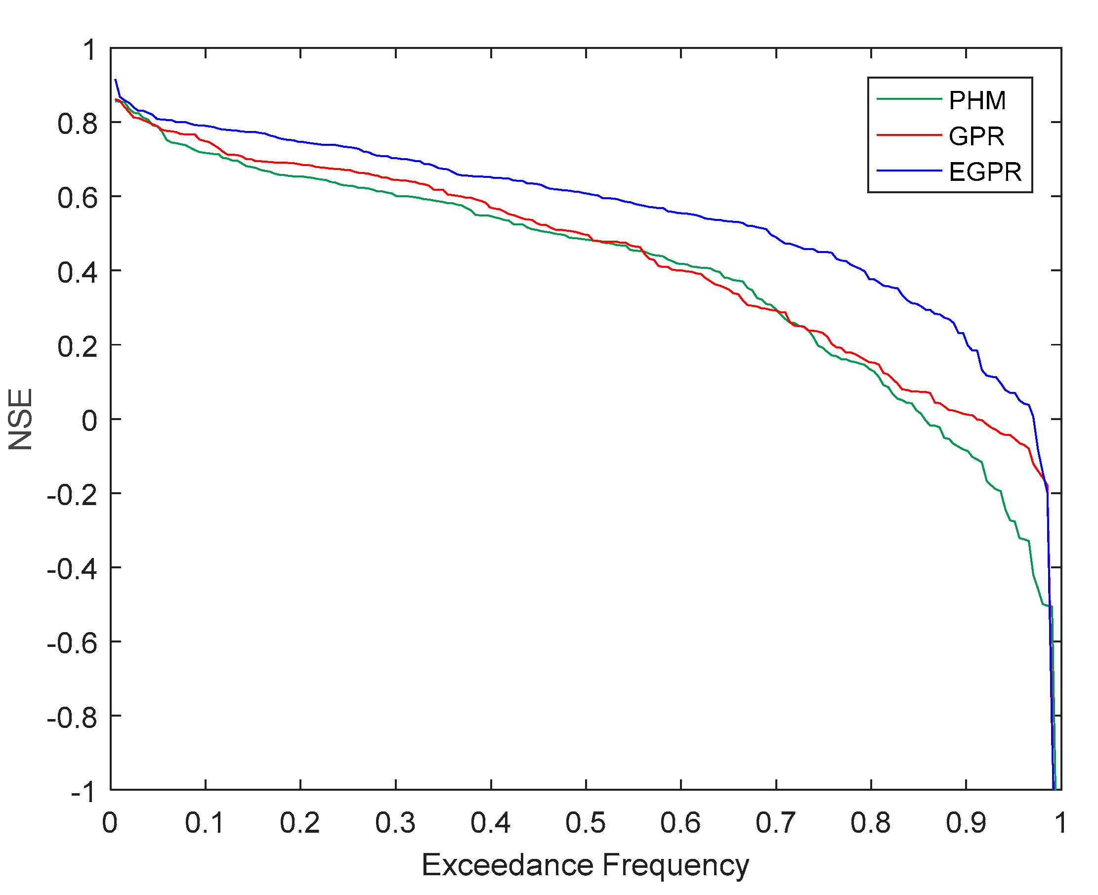
We used the exceedance frequency curve of NSE to show the overall performance of PHM, GPR, and EGPR in 203 MOPEX watersheds in the validation period (Figure 2). PHM and GPR had similar model performance. GPR had slightly better performance, in that it had fewer watersheds with NSE lower than 0. This result indicates that with the same amount of input information, our data-driven model achieved a comparable level of modeling accuracy on simulated monthly surface runoff to our theory-driven conceptual hydrologic model. With the additional input information of potential evaporation and NDVI, selected based on hydrologic knowledge, EGPR had much better performance than both GPR and PHM.
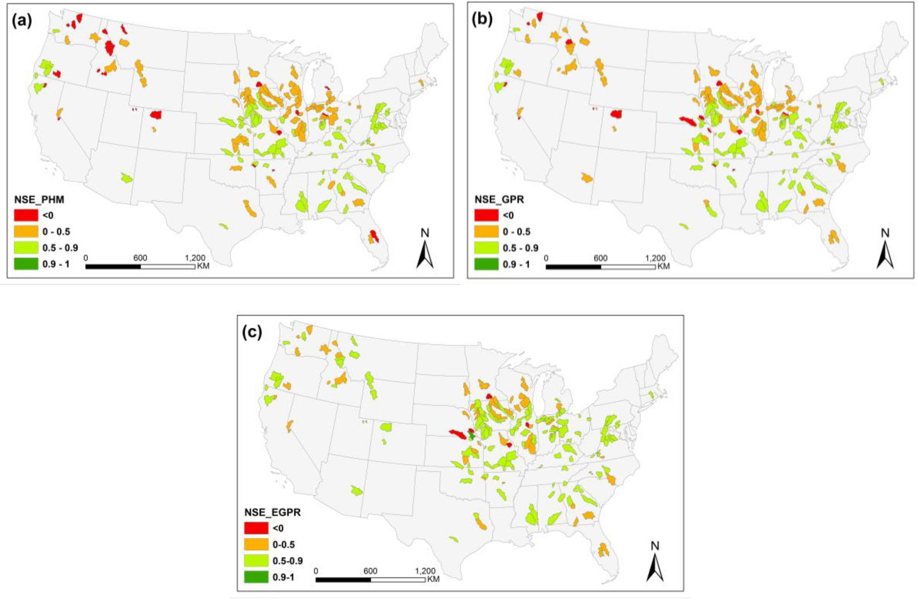
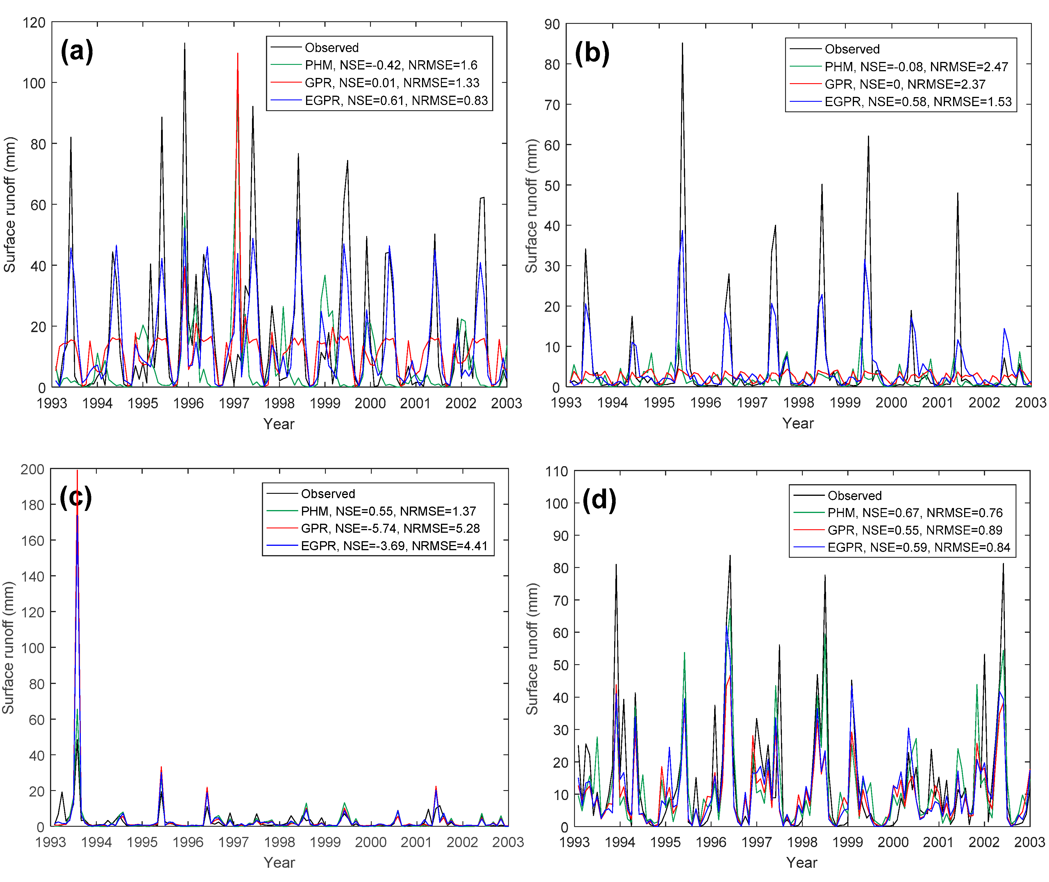
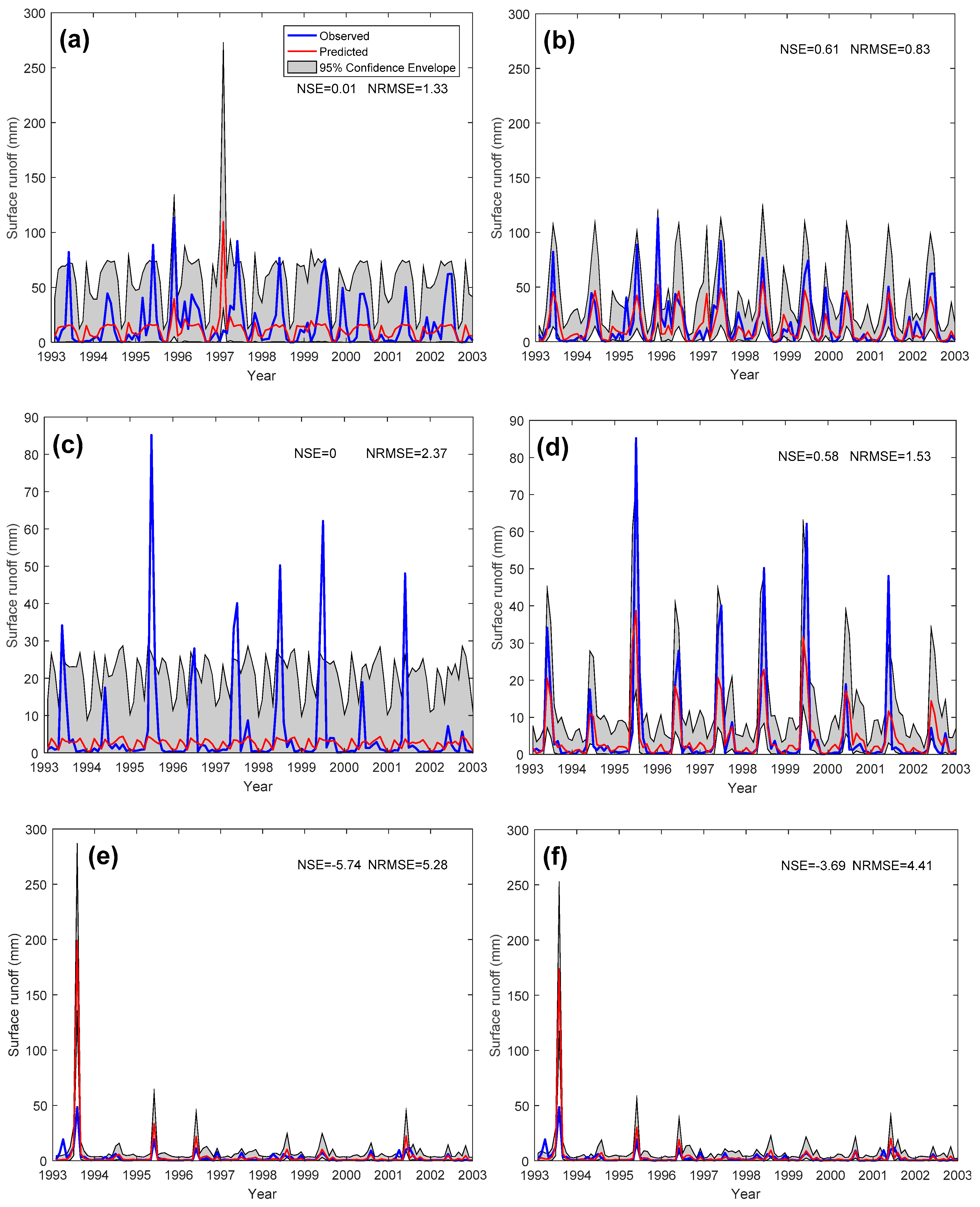
To compare the performance of the three models spatially, we mapped the NSE values of watersheds in the US (Figure 3). Again, GPR and PHM had similar spatial distributions of model performance, while PHM had slightly better performance in the Midwest and GPR had slightly better performance in the Northwest. Performance improvement from GPR to EGPR was found in the Northwest, High Plains, Midwest, and Southeast regions. We selected one watershed in the Northwest region and one in the High Plains region where GPR and EGPR had better performance and two watersheds in the Midwest where PHM had better performance to show the simulation results in time series in the validation period (Figure 4). For the two Western watersheds (Figure 4a,b), both GPR and PHM had weak performance, with PHM having worse NSEs. In both watersheds, GPR underestimated surface runoff peaks, while PHM had trouble capturing the main peaks. EMLM had much better performance than both PHM and GPR. The improvement of EGPR from GPR was mainly due to better accuracy of the peak magnitude estimation. On the other hand, PHM had acceptable performance in the two selected Midwestern watersheds (Figure 4c,d). GPR overestimated the peaks in Little Blue River and underestimated the peaks in East Fork White River. PHM even outperformed EGPR in these two watersheds, especially at Little Blue River. EGPR still had large error on peak magnitude estimation in this region. Based on this comparison, GPR and EGPR did a better job of capturing the timing and magnitude of runoff peaks in the Northwestern regions, while PHM had higher accuracy on peak magnitude estimation in the Midwest.
In general, EGPR had the best performance among the three models, with the highest NSEs and lowest NRMSEs in the 203 MOPEX watersheds across the contiguous US (Table 1).
4.2. Sensitivity Analysis
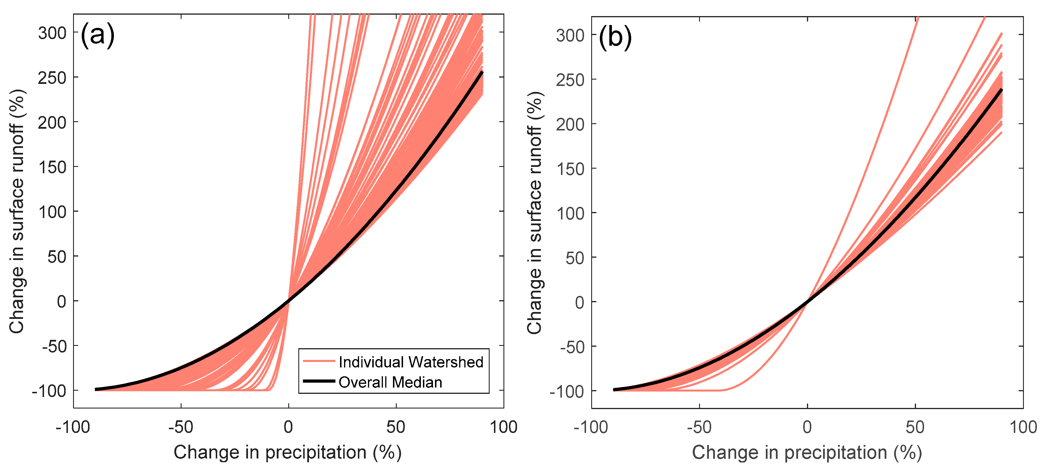
After evaluating the models’ performance, we conducted a sensitivity analysis on each model. Our main objective was to show the sensitivity of surface runoff to the variability of input variables in these three models to gain insight into how the controlling effect of input variables on surface runoff is represented in the models. We employed graphic analysis to examine the effect of each input variable. We first tested the sensitivity of surface runoff to precipitation change in PHM across the 203 study watersheds (Figure 5). Different from performance evaluation, sensitivity analysis was performed for the water-limited season and energy-limited season separately, since PHM simulates the two seasons separately. For both seasons, simulated surface runoff increased with increased precipitation, which was expected based on the form of the PHM equations. Percentage-wise, the sensitivity of surface runoff to precipitation change was higher in water-limited seasons (Figure 5a). Also, the variability of sensitivity among watersheds in water-limited seasons was higher than that in energy-limited seasons. It should be noted that in both seasons, there was a small number of watersheds with negative NSE values, indicating that the surface runoff generation process at these watersheds was not well captured in PHM due to the simplicity of the model structure. These watersheds were eliminated from the PHM sensitivity analysis.
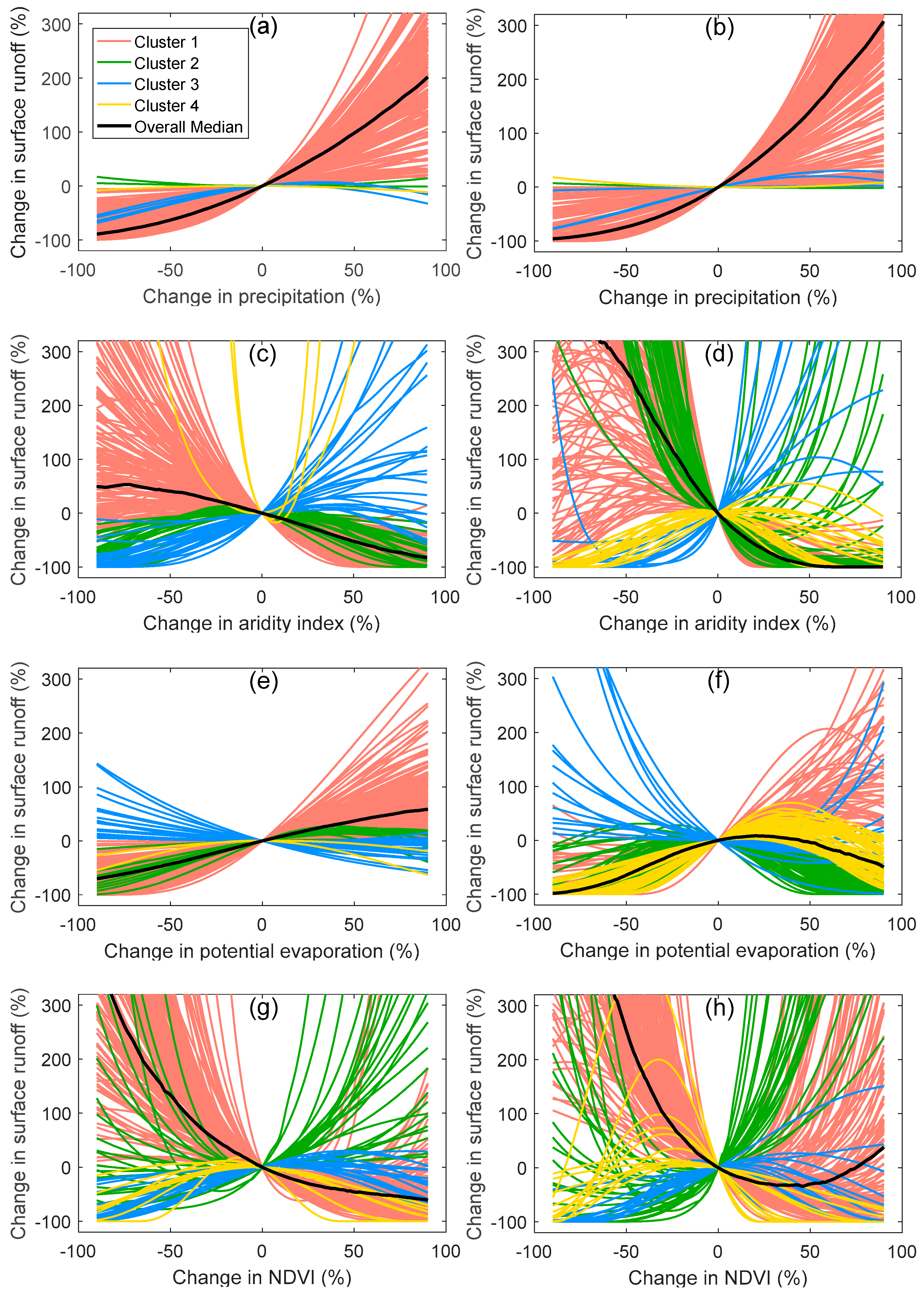
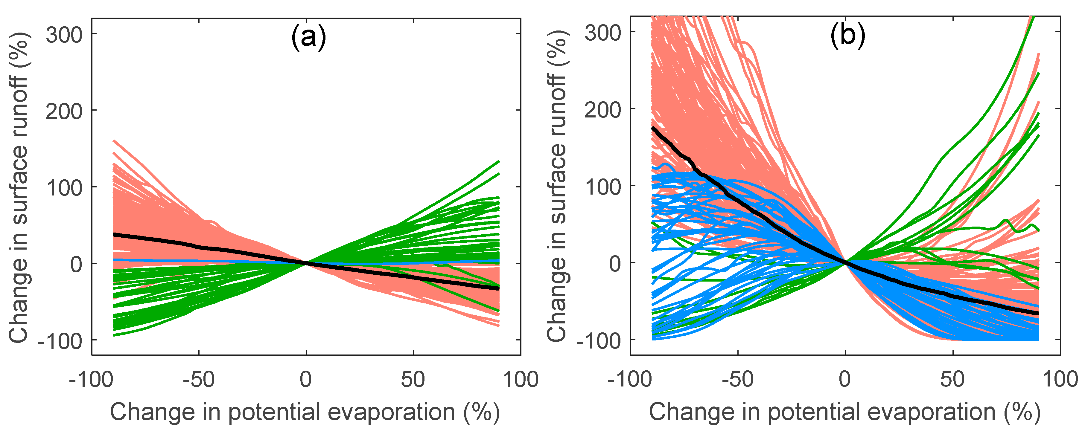
We then tested the sensitivity of surface runoff to each input variable in GPR and EGPR by varying each variable while fixing the other variables at their monthly means (Figure 6 and Figure 7). Similar to PHM, we also eliminated watersheds with negative NSEs in GPR and EGPR. The variability among sensitivity curves in GPR and EGPR was much higher than in PHM. To identify common patterns in these various complicated responses, we conducted clustering analysis on the individual sensitivity curves. We used hierarchical clustering [58] with the correlation distance [59] as the measure of similarity. The correlation distance, given as , where is the correlation between two curves being compared, is an increasing function of the correlation coefficient, hence clustering based on this distance metric groups curves with similar shapes into the same cluster. The resulting clusters are shown as differently colored curves, and the overall median curve is shown in black in Figure 6 and Figure 7. We used three clusters for GPR and four for EGPR. For the sake of comparison, GPR and EGPR sensitivity analysis was also performed on the two seasons separately. In these two models, the responses of surface runoff to changes in precipitation were quite similar, in that surface runoff increased with increased precipitation. The model responses to changes in mean monthly aridity index were more complex. The median trend was still similar in GPR and EGPR, in that surface runoff generally decreased with the increase of aridity index, and sensitivity was higher in energy-limited seasons. However, clusters of curves had different trends from the main trend, which will be discussed along with other clustering results later in this section.
For the two additional inputs in EGPR, the sensitivities of surface runoff to potential evaporation differed depending on the season. During water-limited seasons, the median response of surface runoff to the increase in potential evaporation monotonically increased (Figure 7e), while in energy-limited seasons, the median surface runoff showed an increasing trend first and then changed to a decreasing trend (Figure 7f). In terms of NDVI, the curves are similar to the sensitivity results of aridity index. The median surface runoff response monotonically decreased with the increase of NDVI in water-limited seasons (Figure 7g). In energy-limited seasons, the surface runoff response still mainly decreased with the increase of NDVI. However, at the end, the curve shows an increasing trend. (Figure 7h).
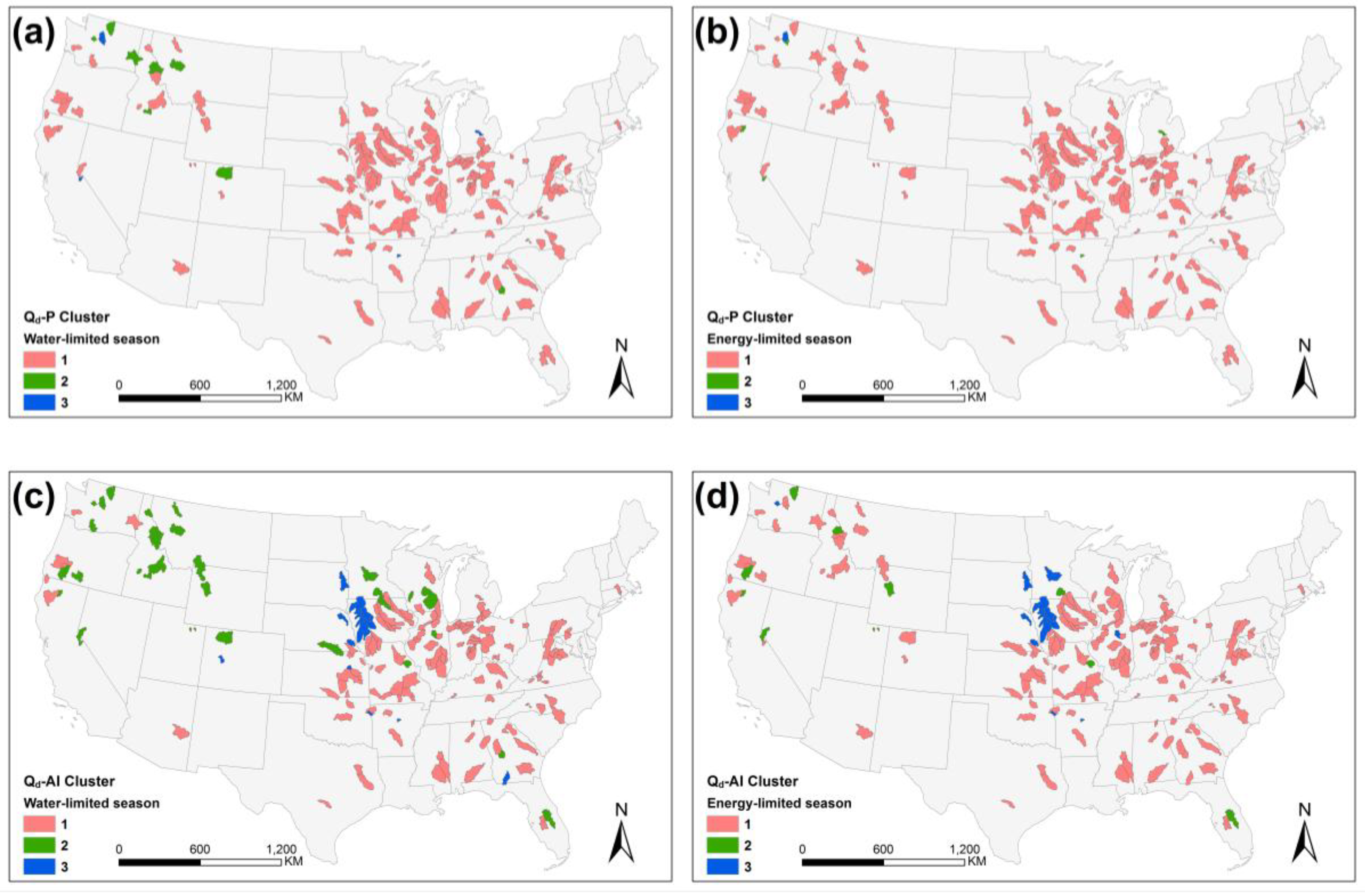
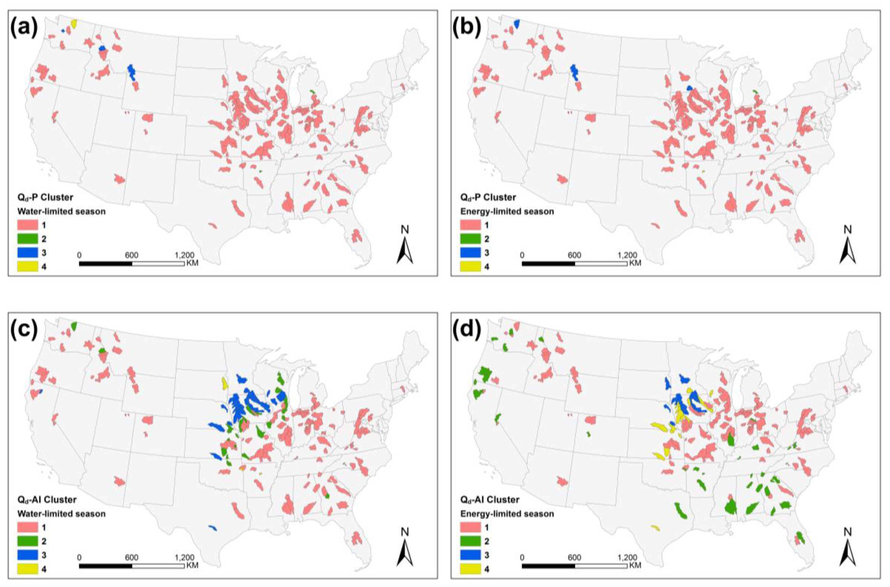
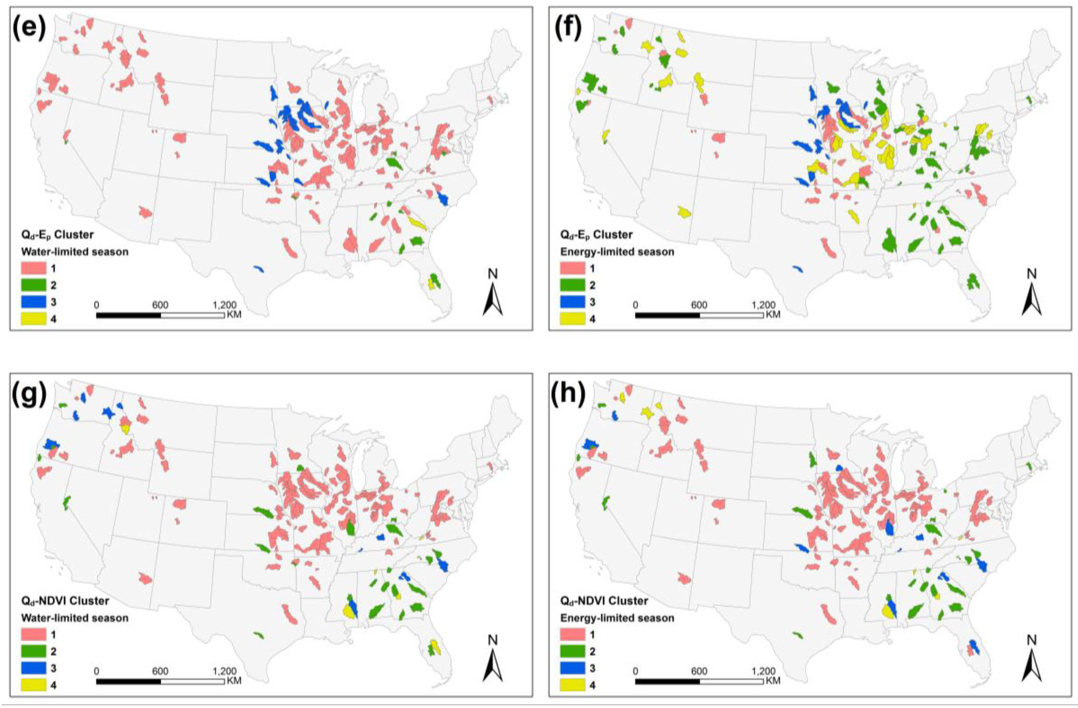
The clustering of response curves provides further insights about the sensitivity differences between the study watersheds. For the increase of surface runoff response to precipitation, both GPR and EGPR had relatively unified patterns of monotonic increase in both seasons, except for a few outliers. The spatial distribution of the clusters shows that these outliers are in the Northern regions (Figure 8 and Figure 9). In terms of mean monthly aridity index, GPR shows a decreasing trend in general, which is represented by the cluster of watersheds in the Eastern and Midwest regions. However, a smaller cluster of watersheds shows an opposite trend of increasing, especially in water-limited seasons, mostly located in the Western regions. Also, some of the Midwest watersheds are in a different cluster from the main one. For EGPR, the mean monthly aridity index cluster pattern is more complex. The difference between watersheds in Eastern and Western regions is not as distinguished as in GPR; instead, the number of clusters of watersheds in the Midwest increased from three to four. The complex clustering in the Midwest may be related to the agricultural activities in this region. Potential evaporation sensitivity clustering is similar to the clustering of mean monthly aridity index, in that some Midwest watersheds are in small clusters that have different trends from the main cluster’s trend. This difference is more significant in energy-limited seasons. Last but not least, the clustering of NDVI sensitivity is slightly different from mean monthly aridity index and potential evaporation sensitivity clustering. Watersheds in the Midwest and Northeast are mostly in one cluster and the Southeastern watersheds are in other clusters. The physical interpretation of the sensitivity results is discussed in Section 5.2.
4.3. Uncertainty Analysis
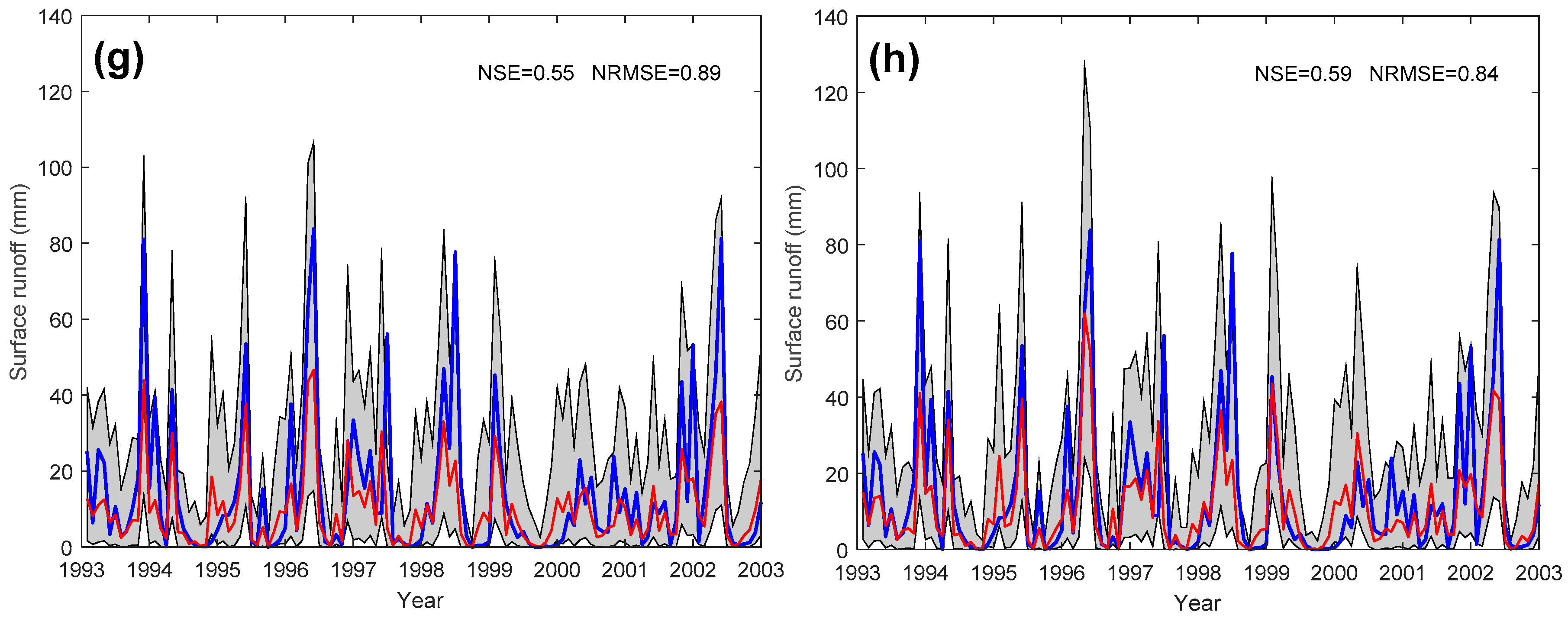
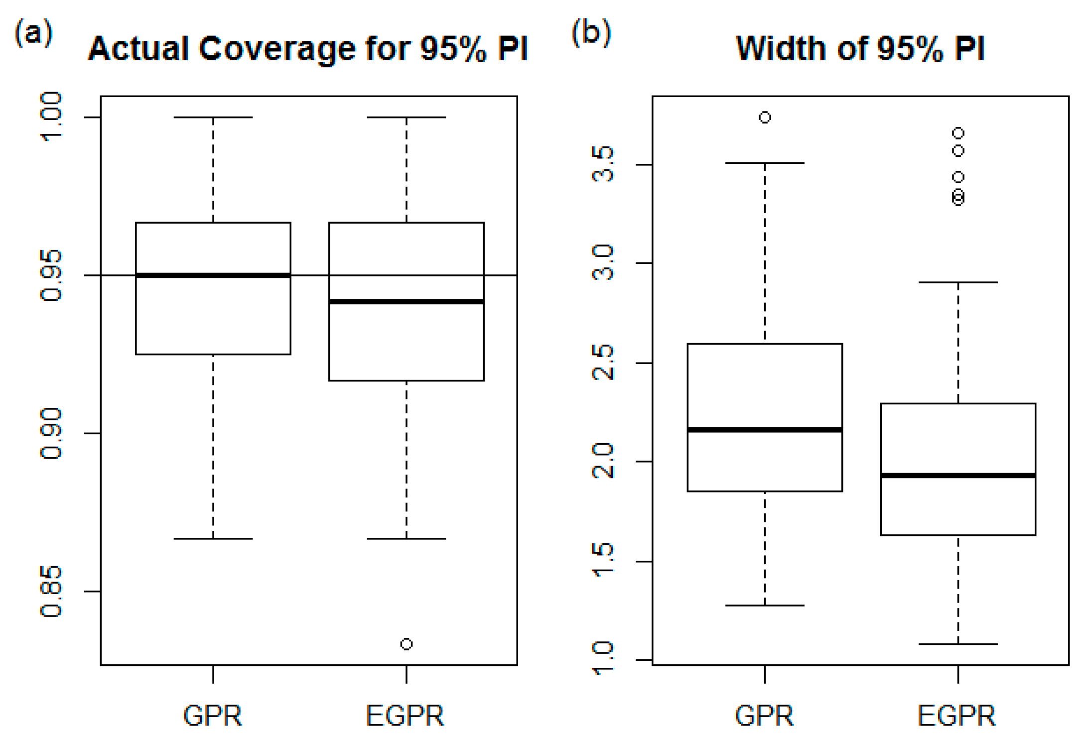
We also investigated how GPR and EGPR perform in terms of uncertainty quantification. We computed 95% prediction intervals for each predicted value in each study watershed. Figure 10 shows the time series of the observed and predicted values and their corresponding 95% prediction intervals for the same four example watersheds as in Figure 4. In these watersheds, especially the first two (Gauge IDs 12459000 and 9292500), the upper limits of the prediction intervals from GPR do not capture the surges in observed surface runoff, while the upper limits from EGPR closely follow the individual peaks in the observed series. Therefore, including the two additional input variables not only increases the prediction accuracy but also improves the uncertainty quantification performance, especially for the higher values of surface runoff. The actual coverage probability and average width were first computed for individual catchments and then converted into box plots to show the distribution of those two quantities among the study watersheds (Figure 11). The results show that both GPR and EGPR have actual coverages that are reasonably close to the nominal 95% coverage. The actual coverage of EGPR seems to be slightly lower, indicating that including the two additional input variables makes it slightly more difficult to obtain well-calibrated prediction intervals. The width of the 95% predication interval (PI) is overall shorter in EGPR, hence using the additional two input variables reduces the prediction uncertainty while maintaining a similar level of actual coverage.
5. Discussion
5.1. Model Performance Comparison
In our comparative study, GPR and PHM show similar performance on simulated monthly surface runoff at watershed scale when given the same amount of input data. PHM uses a physically motivated relationship between surface runoff and precipitation, while GPR learns the relationship between those variables based on the data.
GPR overestimated several summer runoff peaks in the Midwest, as shown in Little Blue River, KS (Gauge ID 6884400), and Little Nemaha River, NE (Gauge ID 6811500). The difficulty of GPR accurately simulating high flows has been reported in previous studies [60], which is related to the dependence of prediction errors on the magnitude of observed values. When the distribution of a variable, such as surface runoff, is highly right-skewed, it is common to observe increased variability for higher magnitudes of values. The prediction error is also affected by this increase of variability. Since we built our prediction model for cubic root transformed data, the prediction errors for the higher variables will be amplified when we transform the data back to the original scale. However, building a model without transformation would also cause modeling problems, such as underestimation of the upper limits. Therefore, despite the error-amplifying effect, cubic root transformation still yields the best modeling performance. In addition, the uncertainty analysis results of GPR show that the observed surface runoff exceeding the upper limit of the 95% prediction interval (3.3%) is reasonably close to the nominal tail probability (2.5%), hence we think that our model still provides a valid prediction of surface runoff.
For Western watersheds, especially in the High Plains region, GPR shows better performance than PHM, in that the timing and magnitude of streamflow peaks are captured better by GPR than by PHM. This result indicates that the form of conceptual equations in PHM may not be suitable for these watersheds, or for the High Plains region in general. As discussed in Chen and Wang [26], the snow effect in cold regions is not considered in this PHM. As a result, the performance in these regions is generally not very good. The snowfall and snow melt processes are different from the rainfall-runoff process, therefore we need to model the snow processes separately, which is beyond the scope of this study.
On the one hand, GPR’s modeling performance relies heavily on the level of representativeness and variability of input data because of its data-driven nature. On the other hand, PHM is based on a set of predefined conceptual equations that may not be capable of capturing rainfall-runoff processes in different watersheds with a wide range of hydrologic characteristics.
The performance of EGPR is much better than both PHM and GPR. The improvement of modeling performance indicates that, besides the original two input variables, the additional two variables selected based on hydrologic knowledge are also major controlling factors of monthly surface runoff variability. We caution that our results do not indicate that simply adding more input variables can improve the simulation performance of our GPR approach. In fact, we have tried to use other monthly variables as input series, such as monthly maximum temperature, monthly precipitation maxima, length of the longest wet spell, and a number of other variables. We found, however, that including these variables did not improve the simulation performance, indicating that they do not contain the same necessary information as the selected variables to predict monthly runoff. It might be tempting to include all available input variables in the machine learning model, but adding redundant variables in GPR often negatively affects the simulation performance by increasing the variance of predicted values [61]. The selection of input variables is therefore crucial to the GPR approach. With only two additional input series selected based on hydrologic knowledge, we significantly improved our GPR’s performance.
To further investigate the reason that EGPR outperformed PHM, we generated a map of the study watersheds with a correlation coefficient between input precipitation and observed surface runoff (Figure 11a). Comparing the performance of PHM and EGPR, PHM works well with watersheds with a strong positive correlation between precipitation and surface runoff but poorly with watersheds with a weak positive or even negative correlation between precipitation and surface runoff. EGPR outperformed PHM in these watersheds, since it has more inputs and a more flexible model structure. Therefore, to improve the model robustness of PHM, we focused on these watersheds with weak positive or negative correlation between precipitation and surface runoff. These watersheds are strongly affected by snow processes [56].
5.2. Physical Interpretation of Sensitivity Analysis Results
The sensitivity analysis results show a variety of clusters of shapes, especially in GPR and EGPR, representing a wide range of responses of monthly surface runoff to the variability of input variables.
First, the results show a monotonic increase of surface runoff with increased precipitation in PHM, GPR, and EGPR models. Across 203 watersheds with different climate and land surface characteristics, the change in strong positive sensitivity of surface runoff to precipitation is consistent. However, there are outliers in the GPR and EGPR analysis results that show negative sensitivity between precipitation and surface runoff. The abnormal pattern of these outliers is also shown in the correlation between input precipitation and observed surface runoff (Figure 12a), which could be due to snow effects.
In terms of mean monthly aridity index, surface runoff had a negative sensitivity trend in general in both GPR and EGPR. This negative trend was more significant in energy-limited seasons. The negative sensitivity of surface runoff to mean monthly aridity was expected based on the complementary Budyko-type relationship [53,62], in which the ratio of runoff to precipitation decreases with increased aridity index. The clustering result of surface runoff sensitivity to mean monthly aridity index shows that the majority of watersheds in the Eastern regions form the main cluster, while watersheds in the Midwest are in small clusters different from the main cluster in both seasons. This result indicates unique watershed behaviors in the Midwest, which could be related to the agricultural activities in this region. This spatial pattern of sensitivity is also consistent with the correlation between input aridity index and observed surface runoff (Figure 12b). It should be noted that the spatial patterns shown in Figure 12b–d are similar, indicating that the input variables of aridity index, potential evaporation, and NDVI have similar effects on surface runoff variability.
For the two additional input variables of EGPR, the positive sensitivity of surface runoff to the change of potential evaporation in the main cluster of watersheds, especially in water-limited seasons, is surprising. This positive trend contradicts the results of some previous studies, which showed that runoff and potential evaporation are negatively correlated [63]. It also contradicts the correlation results shown in Figure 12c. To further investigate the sensitivity of surface runoff to potential evaporation changes, we used only precipitation and potential evaporation as input variables to run an additional machine learning simulation and perform a sensitivity analysis on this additional model following the same procedure. The model shows similar performance to the GPR, with an average NSE of 0.37, and the sensitivity of surface runoff to the increase of potential evaporation became a decreasing trend (Figure 13a,b), which agrees with previous studies. This change of sensitivity trend from increasing to decreasing and the similarity shown in Figure 12b–d indicate that there is confounding among potential evaporation, mean monthly aridity index, and NDVI. That is, potential evaporation is related not only to surface runoff but also to aridity index and vegetation coverage. Therefore, the response of surface runoff to NDVI change is also affected by confounding. Similar to the sensitivity analysis results of the aridity index, the surface runoff response generally decreased with the increase of NDVI (Figure 7g,h). The spatial pattern of surface runoff sensitivity to NDVI can be related to the type of vegetation coverage: Midwest and Northeast regions are covered by temperate deciduous forest, while the Southeast is covered by subtropical evergreen forest.
The confounding between input variables in our models is due to the interconnection between these variables in the hydrologic cycle. Within the four input variables we selected, aridity index, potential evaporation, and NDVI have similar correlation with surface runoff (Figure 12b–d), indicating that their effects are partially overlaid. We also calculated the correlation coefficient r values between the three overlying input variables for each of the 203 watersheds. Across the study watersheds, the average r values of aridity index vs. potential evaporation, aridity index vs. NDVI, and potential evaporation vs. NDVI are 0.78, 0.69, and 0.84, respectively. This result confirms that these three input variables are closely related and therefore their effects on surface runoff are partially overlaid. Even with this confounding issue, the model performance is improved with the help of two additional input variables. This improvement may be due to the nonoverlaid parts of the additional input variables. In other words, despite the confounding issue, the additional two input variables can provide helpful information to improve the modeling performance.
6. Conclusions
In this study, we systematically compared the performance of a theory-driven conceptual PHM and a data-driven GPR model to simulate monthly surface runoff at 203 watersheds across the contiguous US. With the same level of input information and model structure complexity, both models had similar and acceptable performance, indicating that a data-driven approach can achieve a similar level of performance as a theory-driven hydrologic model. Then, we added two more input variables, selected based on hydrologic knowledge, to our data-driven model. This extended data-driven model had better performance than both the conceptual hydrologic model and the original data-driven model.
We also conducted a sensitivity analysis to see the models’ responses to variability of input variables. The result showed that the simulated surface runoff in all three models was positively sensitive to the change of precipitation. On the other hand, the sensitivity analysis showed a confounding effect among mean monthly aridity index, potential evaporation, and NDVI, indicating that these three variables have similar effect on surface runoff response.
In future studies, we will include more streamflow-related processes, such as baseflow generation and snow processes, in our modeling framework. We will also further investigate the confounding effect of aridity index, potential evaporation, and vegetation coverage on surface runoff.
Author Contributions
W.C. developed the machine learning modeling framework and conducted the sensitivity analysis and uncertainty analysis; X.C. contributed to the conceptual modeling part and provided physical interpretation of the study results. All authors contributed equally to the research.
Funding
This research received no external funding.
Acknowledgments
We thank Samuel Zipper at McGill University for giving helpful advice on improving the manuscript. The input data packages can be acquired by contacting the corresponding author.
Conflicts of Interest
The authors declare no conflict of interest.
References
- Maier, H.R.; Dandy, G.C. Neural networks for the prediction and forecasting of water resources variables: A review of modelling issues and applications. Environ. Model. Softw. 2000, 15, 101–123. [Google Scholar] [CrossRef]
- Babovic, V. Data mining in hydrology. Hydrol. Process. 2005, 19, 1511–1515. [Google Scholar] [CrossRef]
- Solomatine, D.P.; Ostfeld, A. Data-driven modelling: Some past experiences and new approaches. J. Hydroinform. 2008, 10, 3–22. [Google Scholar] [CrossRef]
- Maier, H.R.; Jain, A.; Dandy, G.C.; Sudheer, K.P. Methods used for the development of neural networks for the prediction of water resources variables: Current status and future directions. Environ. Model. Softw. 2010, 25, 891–909. [Google Scholar] [CrossRef]
- Elshorbagy, A.; Corzo, G.; Srinivasulu, S.; Solomatine, D.P. Experimental investigation of the predictive capabilities of data driven modeling techniques in hydrology—Part 1: Concepts and methodology. Hydrol. Earth Syst. Sci. 2010, 14, 1931–1941. [Google Scholar] [CrossRef]
- Elshorbagy, A.; Corzo, G.; Srinivasulu, S.; Solomatine, D.P. Experimental investigation of the predictive capabilities of data driven modeling techniques in hydrology—Part 2: Application. Hydrol. Earth Syst. Sci. 2010, 14, 1943–1961. [Google Scholar] [CrossRef]
- Abrahart, R.J.; Anctil, F.; Coulibaly, P.; Dawson, C.W.; Mount, N.J.; See, L.M.; Shamseldin, A.Y.; Solomatine, D.P.; Toth, E.; Wilby, R.L. Two decades of anarchy? Emerging themes and outstanding challenges for neural network river forecasting. Prog. Phys. Geogr. 2012, 36, 480–513. [Google Scholar] [CrossRef]
- Genton, M.G. Classes of kernels for machine learning: A statistics perspective. J. Mach. Learn. Res. 2001, 2, 299–312. [Google Scholar]
- Rasmussen, C.E.; Williams, C.K.I. Gaussian Processes for Machine Learning; The MIT Press: Cambridge, MA, USA, 2006; ISBN 026218253X. [Google Scholar]
- James, G.; Witten, D.; Hastie, T.; Tibshirani, R. An Introduction to Statistical Learning; Springer: New York, NY, USA, 2013. [Google Scholar]
- Alpaydin, E. Introduction to Machine Learning; The MIT Press: Cambridge, MA, USA, 2014. [Google Scholar]
- Witten, I.H.; Frank, E.; Hall, M.A.; Pal, C.J. Data Mining: Practical Machine Learning Tools and Techniques; Morgan Kaufmann Publishers: Burlington, MA, USA, 2016. [Google Scholar]
- Sun, A.Y.; Wang, D.; Xu, X. Monthly streamflow forecasting using Gaussian Process Regression. J. Hydrol. 2014, 511, 72–81. [Google Scholar] [CrossRef]
- Mount, N.J.; Maier, H.R.; Toth, E.; Elshorbagy, A.; Solomatine, D.; Chang, F.; Abrahart, R.J. Data-driven modelling approaches for socio-hydrology: Opportunities and challenges within the Panta Rhei Science Plan. Hydrol. Sci. J. 2016, 61, 1192–1208. [Google Scholar] [CrossRef]
- Mount, N.J.; Abrahart, R.J. Load or concentration, logged or unlogged? Addressing ten years of uncertainty in neural network suspended sediment prediction. Hydrol. Process. 2011, 25, 3144–3157. [Google Scholar] [CrossRef]
- Sudheer, K.P. Knowledge extraction from trained neural network river flow models. J. Hydrol. Eng. 2005, 10, 264–269. [Google Scholar] [CrossRef]
- Nouraini, V.; Fard, M.S. Sensitivity analysis of the artificial neural network outputs in simulation of the evaporation process at different climatologic regines. Adv. Eng. Softw. 2012, 47, 127–146. [Google Scholar] [CrossRef]
- Dawson, C.W.; Mount, N.J.; Abrahart, R.J.; Louis, J. Sensitivity analysis for comparison, validation and physical legitimacy of neural network-based hydrological models. J. Hydroinform. 2014, 16, 407–418. [Google Scholar] [CrossRef] [Green Version]
- Kingston, G.B.; Maier, H.R.; Lambert, M.F. Calibration and validation of neural networks to ensure physically plausible hydrological modeling. J. Hydrol. 2005, 314, 158–176. [Google Scholar] [CrossRef]
- Mount, N.J.; Dawson, C.W.; Abrahart, R.J. Legitimising data-driven models: Exemplification of a new data-driven mechanistic modelling framework. Hydrol. Earth Syst. Sci. 2013, 17, 2827–2843. [Google Scholar] [CrossRef]
- Anctil, F.; Perrin, C.; Andréassian, V. Impact of the length of observed records on the performance of ANN and of conceptual parsimonious rainfall-runoff forecasting models. Environ. Model. Softw. 2004, 19, 357–368. [Google Scholar] [CrossRef]
- Toth, E.; Brath, A. Multistep ahead streamflow forecasting: Role of calibration data in conceptual and neural network modeling. Water Resour. Res. 2007, 43. [Google Scholar] [CrossRef] [Green Version]
- Xu, X.; Yang, D.; Sivapalan, M. Assessing the impact of climate variability on catchment water balance and vegetation cover. Hydrol. Earth Syst. Sci. 2012, 16, 43–58. [Google Scholar] [CrossRef]
- Wang, D.; Alimohammadi, N. Responses of annual runoff, evaporation, and storage change to climate variability at the watershed scale. Water Resour. Res. 2012, 48. [Google Scholar] [CrossRef] [Green Version]
- Chen, X.; Alimohammadi, N.; Wang, D. Modeling interannual variability of seasonal evaporation and storage change based on the extended Budyko framework. Water Resour. Res. 2013, 49, 6067–6078. [Google Scholar] [CrossRef] [Green Version]
- Chen, X.; Wang, D. Modeling seasonal surface runoff and base flow based on the generalized proportionality hypothesis. J. Hydrol. 2015, 527, 367–379. [Google Scholar] [CrossRef]
- Duan, Q.; Schaake, J.; Andreassian, V.; Franks, S.; Goteti, G.; Gupta, H.V.; Gusev, Y.M.; Habets, F.; Hall, A.; Hay, L.; et al. The Model Parameter Estimation Experiment (MOPEX): An overview of science strategy and major results from the second and third workshops. J. Hydrol. 2006, 320, 3–17. [Google Scholar] [CrossRef]
- Nathan, R.J.; McMahon, T.A. Evaluation of automated techniques for base flow and recession analyses. Water Resour. Res. 1990, 26, 1465–1473. [Google Scholar] [CrossRef]
- Zhang, K.; Kimball, J.S.; Nermani, R.R.; Running, S.W. A continuous satellite-derived global record of land surface evapotranspiration from 1983 to 2006. Water Resour. Res. 2010, 46. [Google Scholar] [CrossRef] [Green Version]
- Tucker, C.J.; Pinzon, J.E.; Brown, M.E.; Slayback, D.; Pak, E.W.; Mahoney, R.; Vermote, E.; El Saleous, N. An extended AVHRR 8-km NDVI data set compatible with MODIS and SPOT vegetation NDVI data. Int. J. Remote Sens. 2005, 26, 4485–4498. [Google Scholar] [CrossRef]
- Wang, D.; Tang, Y. A one-parameter Budyko model for water balance captures emergent behavior in Darwinian hydrologic models. Geophys. Res. Lett. 2014, 41, 4569–4577. [Google Scholar] [CrossRef]
- USA Department of Agriculture Soil Conservation Service (USDA SCS). National Engineering Handbook, Section 4: Hydrology; S. Government Printing Office: Washington, DC, USA, 1985.
- Chen, X.; Wang, D.; Tian, F.; Sivapalan, M. From channelization to restoration: Sociohydrologic modeling with changing community preferences in the Kissimmee River Basin, Florida. Water Resour. Res. 2016, 52. [Google Scholar] [CrossRef]
- Stein, M.L. Interpolation of Spatial Data: Some Theory for Kriging; Springer Science & Business Media: Berlin, Germany, 1999. [Google Scholar]
- Sanso, B.; Forest, C.E. Uncertainty quantification: Statistical calibration of climate system properties. J. R. Stat. Soc. Ser. C 2009, 58, 485–503. [Google Scholar] [CrossRef]
- Olson, R.; Sriver, R.; Chang, W.; Haran, M.; Urban, N.M.; Keller, K. What is the effect of unresolved internal climate variability on climate sensitivity estimates? J. Geophys. Res. Atmos. 2013, 118, 4348–4358. [Google Scholar] [CrossRef] [Green Version]
- Chang, W.; Haran, M.; Olson, R.; Keller, K. Fast dimension-reduced climate model calibration and the effect of data aggregation. Ann. Appl. Stat. 2014, 8, 649–673. [Google Scholar] [CrossRef]
- McNeall, D.J.; Challenor, P.G.; Gattiker, J.R.; Stone, E.J. The potential of an observational data set for calibration of a computationally expensive computer model. Geosci. Model Dev. 2013, 6, 1715–1728. [Google Scholar] [CrossRef] [Green Version]
- Chang, W.; Applegate, P.J.; Haran, M.; Keller, K. Probabilistic calibration of a Greenland Ice Sheet model using spatially-resolved synthetic observations: Toward projections of ice mass loss with uncertainties. Geosci. Model Dev. 2014, 7, 1933–1943. [Google Scholar] [CrossRef] [Green Version]
- Chang, W.; Haran, M.; Applegate, P.J.; Pollard, D. Calibrating an ice sheet model using high-dimensional binary spatial data. J. Am. Stat. Assoc. 2016, 111, 57–72. [Google Scholar] [CrossRef]
- Chang, W.; Haran, M.; Applegate, P.J.; Pollard, D. Improving ice sheet model calibration using paleoclimate and modern data. Ann. Appl. Stat. 2016, 10, 2274–2302. [Google Scholar] [CrossRef]
- Pollard, D.; Chang, W.; Haran, M.; Applegate, P.J.; DeConto, R. Large ensemble modeling of last deglacial retreat of the West Antarctic Ice Sheet: Comparison of simple and advanced statistical techniques. Geosci. Model Dev. 2016, 9, 1697–1723. [Google Scholar] [CrossRef]
- Williams, C.K.I. Computation with Infinite Neural Networks. Neural Comput. 1998, 10, 1203–1216. [Google Scholar] [CrossRef] [Green Version]
- Nychka, D.W. Spatial-Process Estimates as Smoothers. In Smoothing and Regression: Approaches, Computation, and Application; Schimek, M.G., Ed.; Wiley: New York, NY, USA, 2000; pp. 393–424. [Google Scholar]
- Goodfellow, I.; Bengio, Y.; Courville, A.; Bengio, Y. Deep Learning; The MIT Press: Cambridge, MA, USA, 2016. [Google Scholar]
- Guyon, I.; Elisseeff, A. An introduction to variable and feature selection. J. Mach. Learn. Res. 2003, 3, 1157–1182. [Google Scholar] [CrossRef]
- Bowden, G.J.; Maier, H.R.; Dandy, G.C. Input determination for neural network models in water resources applications. Part 1. Background and methodology. J. Hydrol. 2005, 301, 75–92. [Google Scholar] [CrossRef]
- May, R.J.; Maier, H.R.; Dandy, G.C.; Fernando, T.M.K.G. Non-linear variable selection for artificial neural networks using partial mutual information. Environ. Model. Softw. 2008, 23, 1312–1326. [Google Scholar] [CrossRef]
- May, R.J.; Dandy, G.C.; Maier, H.R. Review of Input Variable Selection Methods for Artificial Neural Networks; InTech: Rijeka, Croatia, 2011. [Google Scholar]
- Galelli, S.; Castelletti, A. Tree-based iterative input variable selection for hydrological modelling. Water Resour. Res. 2013, 49, 4295–4310. [Google Scholar] [CrossRef]
- Talei, A.; Chua, L.H.C. Influence of lag time on event-based rainfall-runoff modeling using the data driven approach. J. Hydrol. 2012, 438, 223–233. [Google Scholar] [CrossRef]
- He, J.; Valeo, C.; Chu, A.; Neumann, N.F. Prediction of event-based stormwater runoff quantity and quality by ANNs developed using PMI-based input selection. J. Hydrol. 2011, 400, 10–23. [Google Scholar] [CrossRef]
- Budyko, M.I. Climate and Life; Academic Press: New York, NY, USA, 1974. [Google Scholar]
- Thomas, H.A. Final Report: Improved Methods for National Water Assessment. Water Resources Contract: WR15249270; Harvard Water Resources Group: Cambridge, MA, USA, 1981. [Google Scholar]
- Bergström, S. The HBV Model: Its Structure and Applications; Swedish Meteorological and Hydrological Institute: Norrköping, Sweden, 1992. [Google Scholar]
- Martinez, G.F.; Gupta, H.V. Toward improved identification of hydrological models: A diagnostic evaluation of the “abcd” monthly water balance model for the conterminous United States. Water Resour. Res. 2010, 46. [Google Scholar] [CrossRef]
- Nash, J.E.; Sutcliffe, J.V. River flow forecasting using conceptual models part Ⅰ—A discussion of principles. J. Hydrol. 1970, 10, 280–290. [Google Scholar] [CrossRef]
- Montero, P.; Vilar, J. TSclust: An R Package for Time Series Clustering. J. Stat. Softw. 2014, 62, 1–43. [Google Scholar] [CrossRef]
- Golay, X.; Kollias, S.; Stoll, G.; Meier, D.; Valavanis, A.; Boesiger, P. A new correlation based fuzzy logic clustering algorithm for fMRI. Magn. Reson. Med. 1998, 40, 249–260. [Google Scholar] [CrossRef] [PubMed]
- Shortridge, J.E.; Guikema, S.D.; Zaitchik, B.F. Machine learning methods for empirical streamflow simulation: A comparison of model accuracy, interpretability, and uncertainty in seasonal watersheds. Hydrol. Earth Syst. Sci. 2016, 20, 2611–2628. [Google Scholar] [CrossRef]
- Hastie, T.; Tibshirani, R.; Friedman, J. The Elements of Statistical Learning: Data Mining, Inference and Prediction, 2nd ed.; Springer: Berlin, Germany, 2009. [Google Scholar]
- Wang, D.; Wu, L. Similarity of climate control on base flow and perennial stream density in the Budyko framework. Hydrol. Earth Syst. Sci. 2013, 17, 315–324. [Google Scholar] [CrossRef] [Green Version]
- Roderick, M.L.; Farquhar, G.D. A simple framework for relating variations in runoff to variations in climatic conditions and catchment properties. Water Resour. Res. 2011, 47. [Google Scholar] [CrossRef] [Green Version]
Figure 1.
The 203 study watersheds selected for this study from the Model Parameter Estimation Experiment (MOPEX) database with a wide range of mean annual aridity index.
Figure 1.
The 203 study watersheds selected for this study from the Model Parameter Estimation Experiment (MOPEX) database with a wide range of mean annual aridity index.

Figure 2.
Exceedance frequency curves of Nash–Sutcliffe efficiency (NSE) values of proportionality hydrologic model (PHM), Gaussian process regression (GPR), and extended Gaussian process regression (EGPR) simulations.
Figure 2.
Exceedance frequency curves of Nash–Sutcliffe efficiency (NSE) values of proportionality hydrologic model (PHM), Gaussian process regression (GPR), and extended Gaussian process regression (EGPR) simulations.

Figure 3.
Spatial distribution of NSE values in MOPEX in the continental US: (a) PHM, (b) GPR, and (c) EGPR.
Figure 3.
Spatial distribution of NSE values in MOPEX in the continental US: (a) PHM, (b) GPR, and (c) EGPR.

Figure 4.
Comparison of runoff simulation results between PHM, GPR, and EGPR in time series. (a) Wenatchee River, WA (Gauge ID 12459000); (b) Yellowstone River, UT (Gauge ID 9292500); (c) Little Blue River, KS (Gauge ID 6884400); (d) East Fork White River, IN (Gauge ID 3365500).
Figure 4.
Comparison of runoff simulation results between PHM, GPR, and EGPR in time series. (a) Wenatchee River, WA (Gauge ID 12459000); (b) Yellowstone River, UT (Gauge ID 9292500); (c) Little Blue River, KS (Gauge ID 6884400); (d) East Fork White River, IN (Gauge ID 3365500).

Figure 5.
PHM simulated surface runoff sensitivity to precipitation change in study watersheds with positive NSE values in (a) water-limited season and (b) energy-limited season. In order to show the main trend, median curves are highlighted as black lines.
Figure 5.
PHM simulated surface runoff sensitivity to precipitation change in study watersheds with positive NSE values in (a) water-limited season and (b) energy-limited season. In order to show the main trend, median curves are highlighted as black lines.

Figure 6.
GPR sensitivity to change in each input variable of all 203 watersheds in (a,c) water-limited season and (b,d) energy-limited season. Different colors show the cluster memberships of individual curves.
Figure 6.
GPR sensitivity to change in each input variable of all 203 watersheds in (a,c) water-limited season and (b,d) energy-limited season. Different colors show the cluster memberships of individual curves.

Figure 7.
EGPR sensitivity to change in each input variable of all 203 watersheds in (a,c,e,g) water-limited season, and (b,d,f,h) energy-limited season. Different colors show the cluster memberships of individual curves.
Figure 7.
EGPR sensitivity to change in each input variable of all 203 watersheds in (a,c,e,g) water-limited season, and (b,d,f,h) energy-limited season. Different colors show the cluster memberships of individual curves.

Figure 8.
Spatial distribution of watershed clustering in GPR, including surface runoff (Qd) sensitivity to precipitation (P) in (a) water-limited seasons and (b) energy-limited seasons; and surface runoff sensitivity to mean monthly aridity index (AI) in (c) water-limited seasons and (d) energy-limited seasons.

Figure 9.
Spatial distribution of watershed clustering in EGPR, including surface runoff sensitivity to (a) precipitation, (c) mean monthly aridity index, (e) potential evaporation (Ep) and (g) NDVI in water-limited seasons and (b,d,f,h) in energy-limited seasons.
Figure 9.
Spatial distribution of watershed clustering in EGPR, including surface runoff sensitivity to (a) precipitation, (c) mean monthly aridity index, (e) potential evaporation (Ep) and (g) NDVI in water-limited seasons and (b,d,f,h) in energy-limited seasons.


Figure 10.
Prediction intervals for GPR (left panels) and EGPR (right panels) for (a,b) Wenatchee River, WA (Gauge ID 12459000); (c,d) Yellowstone River, UT (Gauge ID 9292500); (e,f) Little Blue River, KS (Gauge ID 6884400); and (g,h) East Fork White River, IN (Gauge ID 3365500).
Figure 10.
Prediction intervals for GPR (left panels) and EGPR (right panels) for (a,b) Wenatchee River, WA (Gauge ID 12459000); (c,d) Yellowstone River, UT (Gauge ID 9292500); (e,f) Little Blue River, KS (Gauge ID 6884400); and (g,h) East Fork White River, IN (Gauge ID 3365500).


Figure 11.
Box plots for catchment-wise (a) actual coverage and (b) width of 95% prediction interval for all watersheds with NSE > 0.
Figure 11.
Box plots for catchment-wise (a) actual coverage and (b) width of 95% prediction interval for all watersheds with NSE > 0.

Figure 12.
Correlation coefficient between surface runoff observation and input variables of (a) precipitation, (b) aridity index, (c) potential evaporation, and (d) NDVI.
Figure 12.
Correlation coefficient between surface runoff observation and input variables of (a) precipitation, (b) aridity index, (c) potential evaporation, and (d) NDVI.

Figure 13.
Additional GPR using precipitation and potential evaporation as input variables. Sensitivity to changes of potential evaporation in all 203 watersheds in (a) water-limited seasons and (b) energy-limited seasons. Different colors show the cluster memberships of individual curves.
Figure 13.
Additional GPR using precipitation and potential evaporation as input variables. Sensitivity to changes of potential evaporation in all 203 watersheds in (a) water-limited seasons and (b) energy-limited seasons. Different colors show the cluster memberships of individual curves.


Table 1.
Number of watersheds in each quantile of NSE and normalized root mean square error (NRMSE) values and mean NSE and NRMSE values of PHM, GPR, and EGPR.
Table 1.
Number of watersheds in each quantile of NSE and normalized root mean square error (NRMSE) values and mean NSE and NRMSE values of PHM, GPR, and EGPR.
| Model | NSE | NRMSE | ||||||||
|---|---|---|---|---|---|---|---|---|---|---|
| <0 | 0–0.5 | 0.5–0.9 | 0.9–1 | Mean | 0–0.5 | 0.5–1 | 1–2 | >2 | Mean | |
| PHM | 30 | 79 | 94 | 0 | 0.38 | 0 | 94 | 103 | 6 | 1.14 |
| GPR | 19 | 84 | 100 | 0 | 0.39 | 1 | 100 | 94 | 8 | 1.15 |
| EGPR | 6 | 57 | 139 | 1 | 0.52 | 3 | 124 | 72 | 4 | 1.01 |
© 2018 by the authors. Licensee MDPI, Basel, Switzerland. This article is an open access article distributed under the terms and conditions of the Creative Commons Attribution (CC BY) license (http://creativecommons.org/licenses/by/4.0/).
Share and Cite
MDPI and ACS Style
Chang, W.; Chen, X. Monthly Rainfall-Runoff Modeling at Watershed Scale: A Comparative Study of Data-Driven and Theory-Driven Approaches. Water 2018, 10, 1116. https://doi.org/10.3390/w10091116
AMA Style
Chang W, Chen X. Monthly Rainfall-Runoff Modeling at Watershed Scale: A Comparative Study of Data-Driven and Theory-Driven Approaches. Water. 2018; 10(9):1116. https://doi.org/10.3390/w10091116
Chicago/Turabian StyleChang, Won, and Xi Chen. 2018. "Monthly Rainfall-Runoff Modeling at Watershed Scale: A Comparative Study of Data-Driven and Theory-Driven Approaches" Water 10, no. 9: 1116. https://doi.org/10.3390/w10091116
Note that from the first issue of 2016, this journal uses article numbers instead of page numbers. See further details here.