Flood Routing in River Reaches Using a Three-Parameter Muskingum Model Coupled with an Improved Bat Algorithm


 ,
, 
Abstract
:1. Introduction
1.1. Background
1.2. Problem Statement
1.3. Objective
2. Materials and Methods
2.1. Flood Routing
- Consider initial values for parameters K, X, , and m and enter them into the optimization algorithm, in the form of initial population.
- Calculate the storage based on Equation (3), assuming the equality of input and output flow.
- Calculate the change in storage relative to time, based on Equation (5).
- Calculate the storage based on t + 1, according to Equation (6).
- Calculate the output flow at t + 1, based on Equation (4).
- Repeat steps 2 to 5.
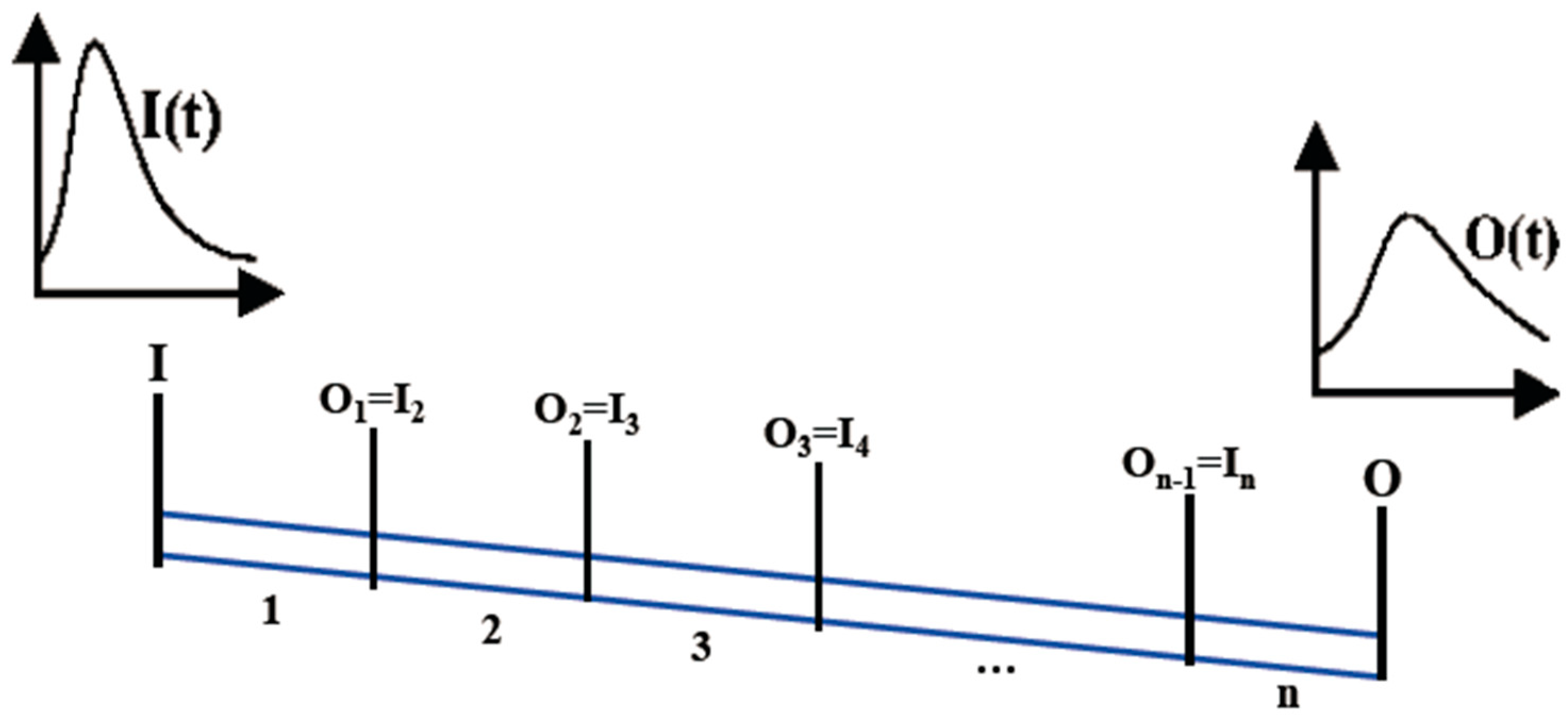
2.2. Optimization of Multi-Reach Muskingum Coefficients
2.3. BAT Algorithm
- All bats have a high ability to receive sound, so that they can detect food after producing loud sounds.
- Bats fly randomly at a velocity at place yl, capable of producing sound with fmin frequency and wavelength. The sound produced by bats also has loudness .
- The loudness of sound, of the bats ranges from to .
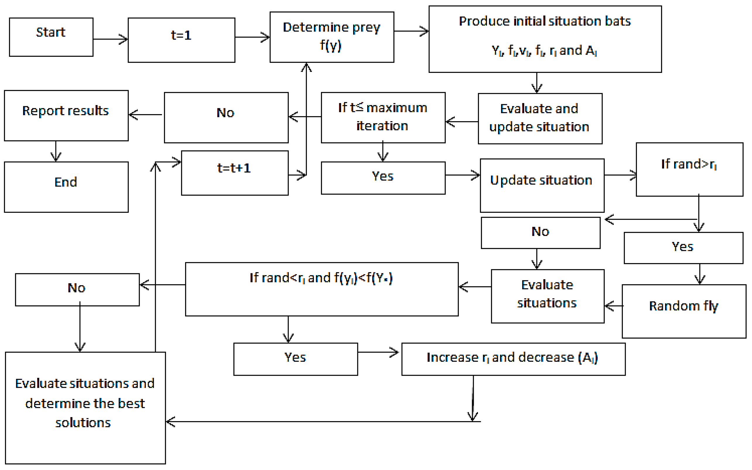
2.4. Improved Bat Algorithm (IBA)
- Adjust the random parameters for the algorithm, such as loudness, pulsation rate, frequency, and other parameters.
- The individual position is computed using Equations (13)–(15), and then the objective function is computed for each member, and the best solution is considered as .
- The frequency and velocity are updated using Equations (7) and (8), and the position is computed using Equation (17).
- The randomness value is compared with rl, and if rl is less than the randomness value, the distribution of the best position is acted based on 0.01 times the random disturbance.
- The local search is considered for this level. If the loudness is less than rand, the loudness should be updated and the pulsation rate should be improved using Equation (12).
- Compute the objective function and change the range using Equation (16).
- The convergence criterion is checked and if it is satisfied, the algorithm finishes or else the algorithm goes to step 2.
2.5. Genetic Algorithm (GA)
2.6. Particle Swarm Algorithm (PSO)
Indices of Error Measurement
3. Results and Discussion
3.1. Wilson Flood
3.2. Multi-Interval Flood Routing (Wilson Flood)
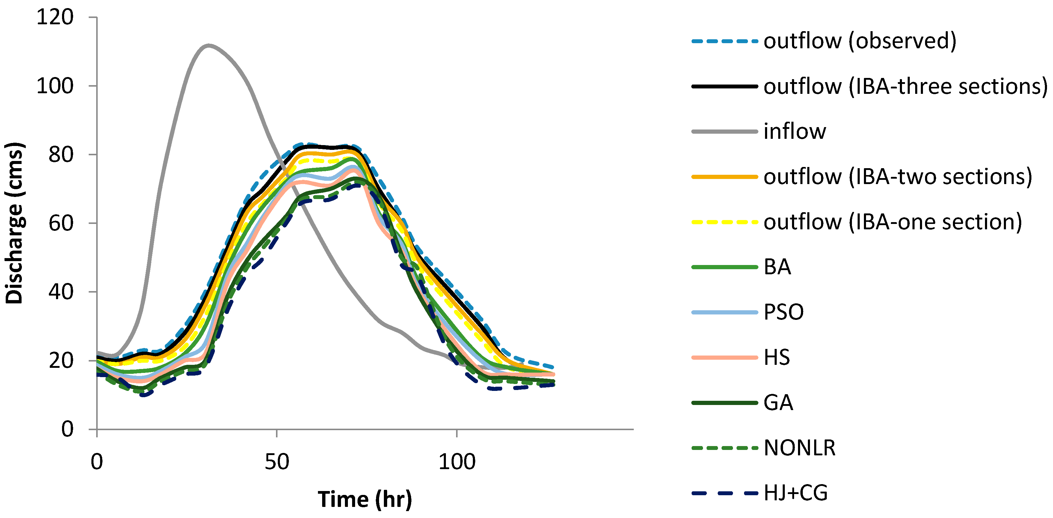
3.3. Karahan Flood
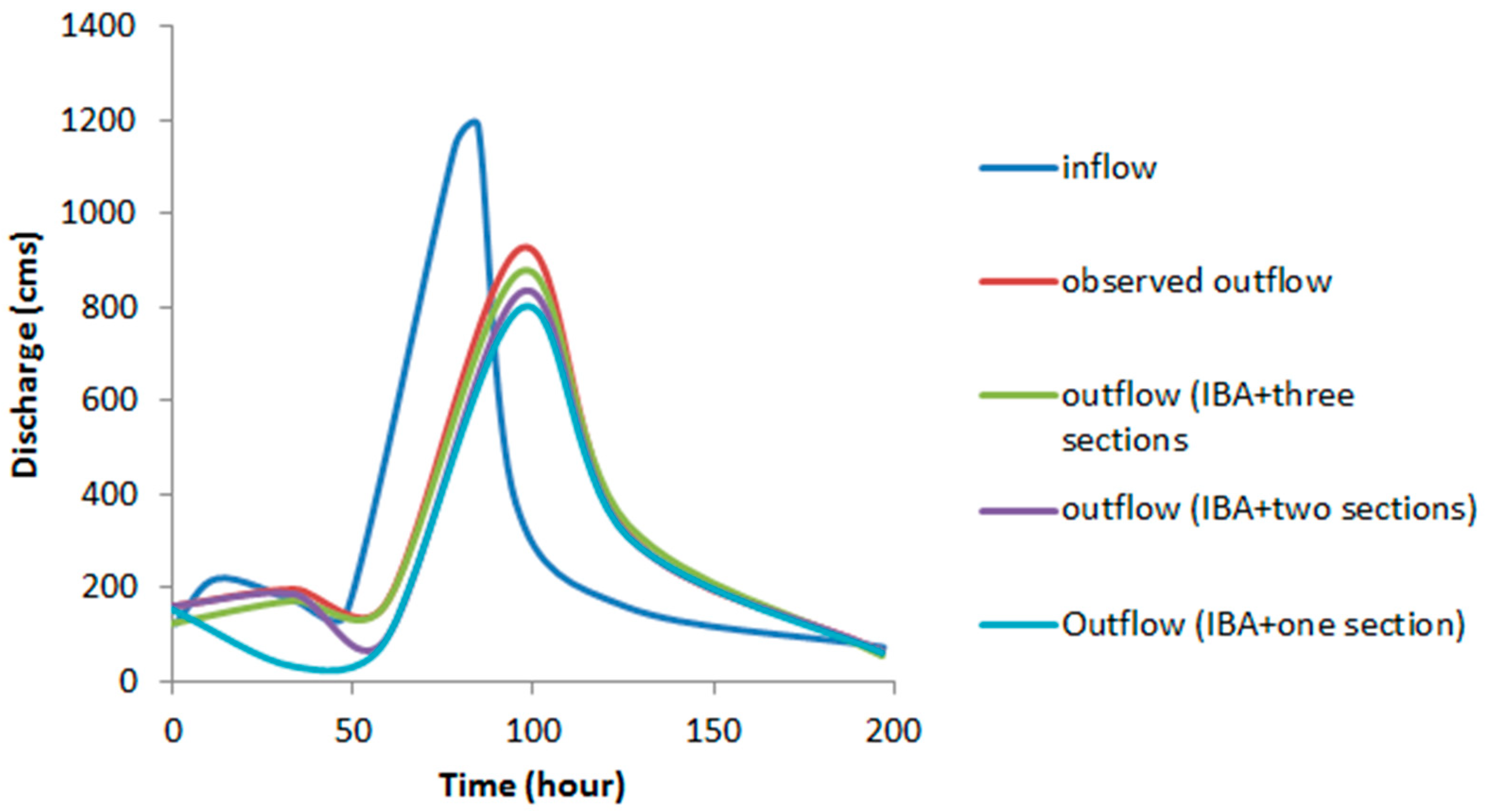
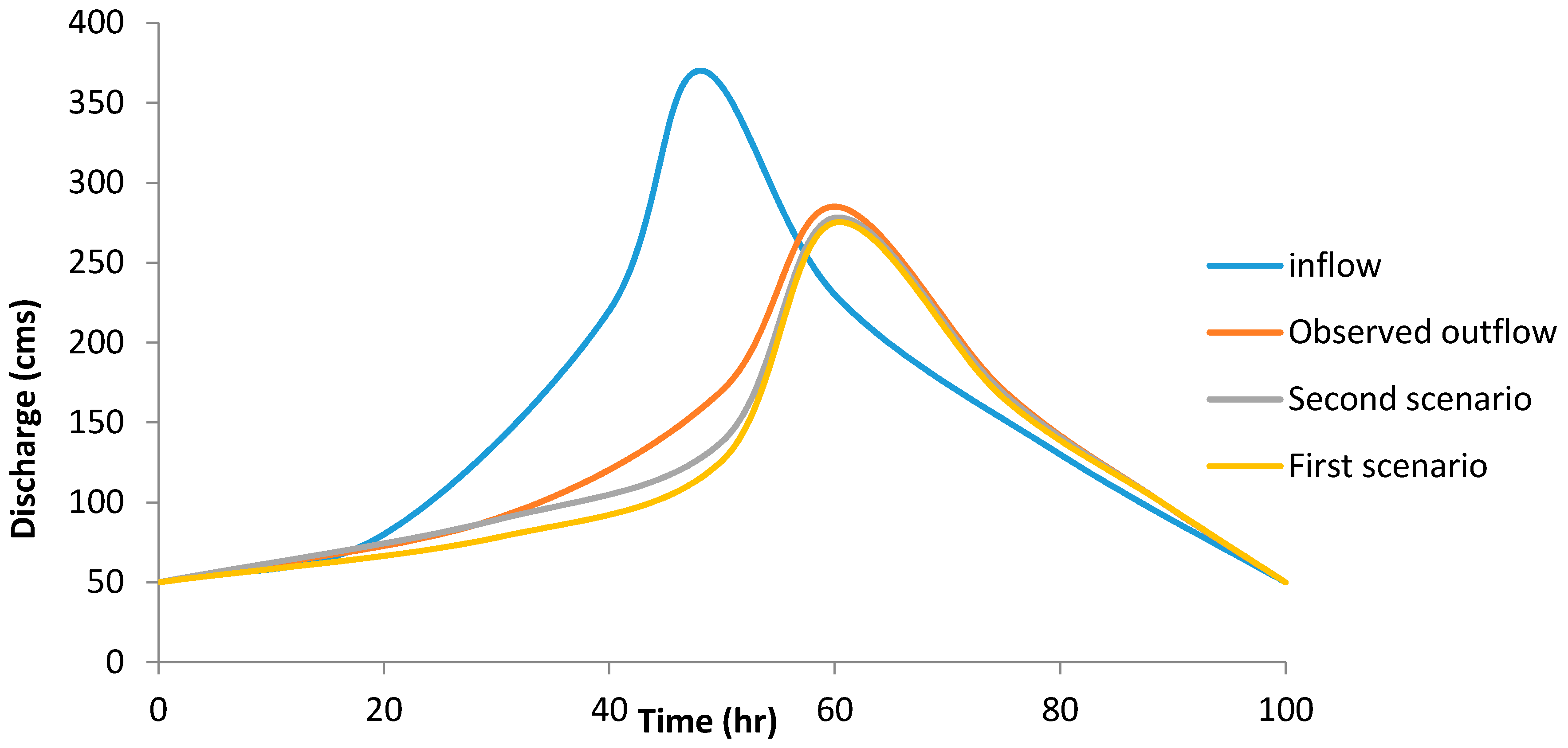
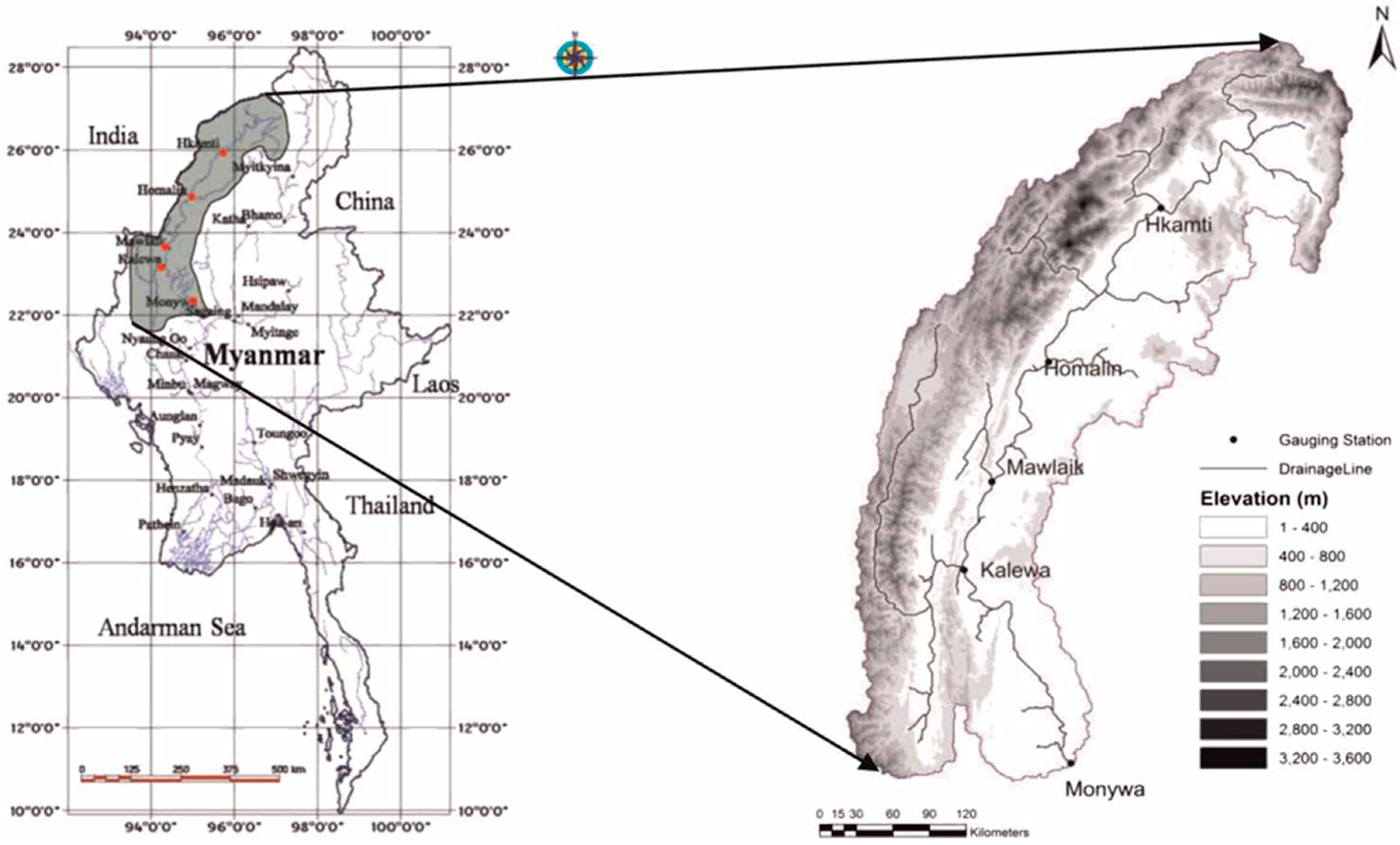
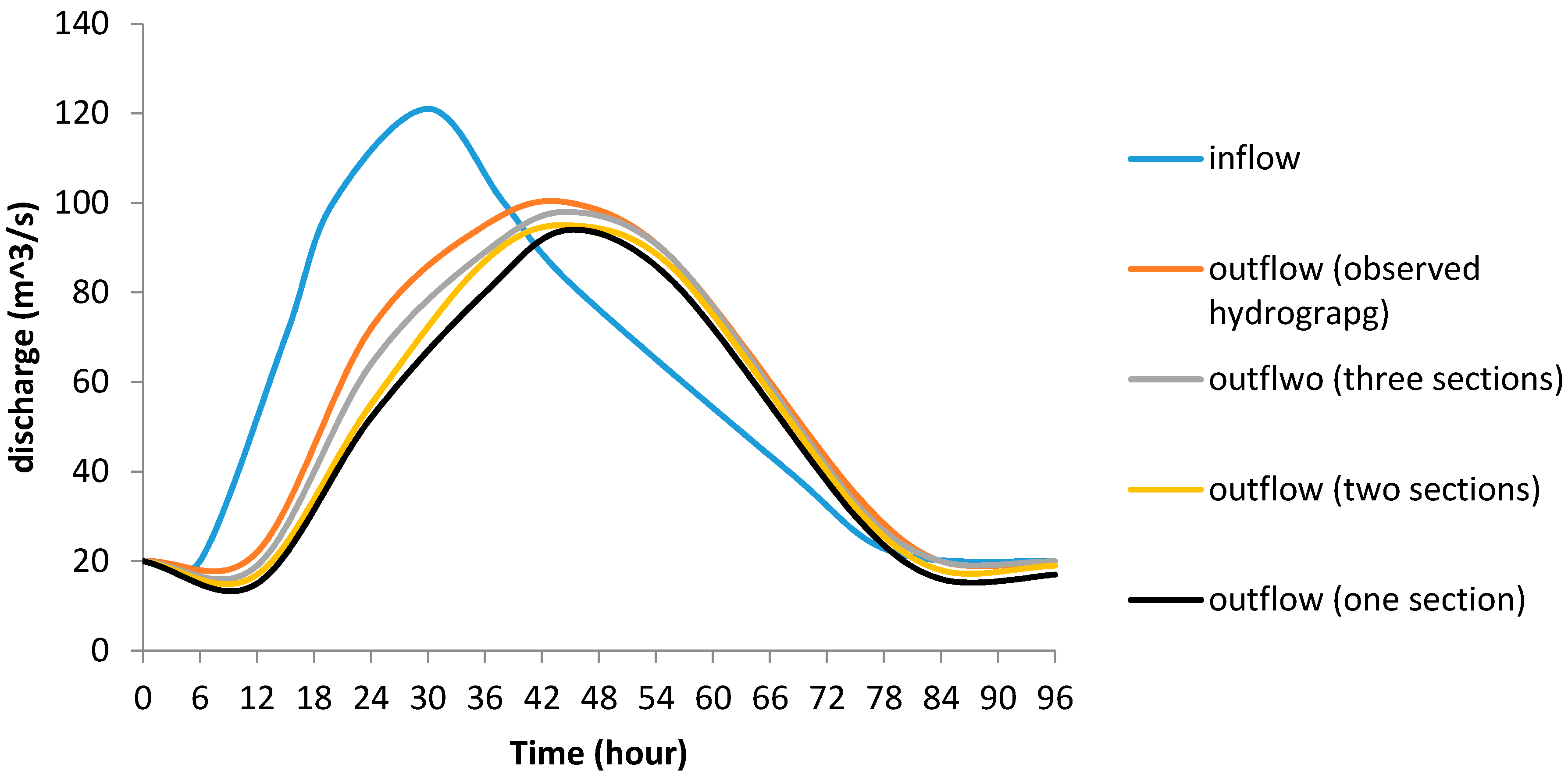
3.4. Chindwin River
4. Conclusions
Author Contributions
Funding
Acknowledgments
Conflicts of Interest
Abbreviations
| IBA | Improved Bat Algorithm |
| GA | Genetic Algorithm |
| PSO | Particle Swarm Optimization |
| PS | Pattern Search |
| HS | Harmony Search |
| HBMO | Honey Bee Mating Optimization |
| NMSA | Nelder-Mead Simplex Algorithm |
| GPA | Genetic Programming Algorithm |
| RMSE | Root Mean Square Error |
| MAE | Mean Absolute Error |
| HA | Harmony Algorithm |
| FLA | Frog Leaping Algorithm |
| (IHBA) | Improved Honey Bee Algorithm |
| (IWOA) | Invasive Weed Optimization Algorithm |
| (BA) | Bat Algorithm |
| BI | Bat Intelligence |
| TPMM | Three-Parameter Muskingum method |
| SSD | Sum of Squares |
| SAD | Sum of Absolute Deviations |
| EP | Error of Peak |
| ETP | Error of Time to Peak |
References
- Barati, R.; Badfar, M.; Azizyan, G.; Akbari, G.H. Discussion of “Parameter Estimation of Extended Nonlinear Muskingum Models with the Weed Optimization Algorithm” by Farzan Hamedi, Omid Bozorg-Haddad, Maryam Pazoki, Hamid-Reza Asgari, Mehran Parsa, and hugo a. Loáiciga. J. Irrig. Drain. Eng. 2018, 144, 7017021. [Google Scholar] [CrossRef]
- Hamedi, F.; Bozorg-Haddad, O.; Pazoki, M.; Asgari, H.R.; Parsa, M.; Loáiciga, H.A. Parameter estimation of extended nonlinear muskingum models with the weed optimization algorithm. J. Irrig. Drain. Eng. 2016, 142, 4016059. [Google Scholar] [CrossRef]
- Zhang, S.; Kang, L.; Conservation, B.Z. Parameter estimation of nonlinear muskingum model with variable exponent using adaptive genetic algorithm. In Environmental Conservation, Clean Water, Air & Soil (CleanWAS); IWA Publishing: London, UK, 2017; pp. 231–234. [Google Scholar]
- Bradbrook, K.F.; Lane, S.N.; Waller, S.G.; Bates, P.D. Two dimensional diffusion wave modelling of flood inundation using a simplified channel representation. Int. J. River Basin Manag. 2004, 2, 211–223. [Google Scholar] [CrossRef]
- Neal, J.; Villanueva, I.; Wright, N.; Willis, T.; Fewtrell, T.; Bates, P. How much physical complexity is needed to model flood inundation? Hydrol. Process. 2012, 26, 2264–2282. [Google Scholar] [CrossRef]
- Hunter, N.M.; Bates, P.D.; Neelz, S.; Pender, G.; Villanueva, I.; Wright, N.G.; Liang, D.; Falconer, R.A.; Lin, B.; Waller, S.; et al. Benchmarking 2D hydraulic models for urban flooding simulations. Proc. Inst. Civ. Eng. Water Manag. 2008, 161, 13–30. [Google Scholar] [CrossRef] [Green Version]
- Dottori, F.; Todini, E. Testing a simple 2D hydraulic model in an urban flood experiment. Hydrol. Process. 2013, 27, 1301–1320. [Google Scholar] [CrossRef]
- Kim, B.; Sanders, B.F.; Schubert, J.E.; Famiglietti, J.S. Mesh type tradeoffs in 2D hydrodynamic modeling of flooding with a godunov-based flow solver. Adv. Water Resour. 2014, 68, 42–61. [Google Scholar] [CrossRef]
- Prestininzi, P. Suitability of the diffusive model for dam break simulation: Application to a cadam experiment. J. Hydrol. 2008, 361, 172–185. [Google Scholar] [CrossRef]
- Aricò, C.; Sinagra, M.; Begnudelli, L.; Tucciarelli, T. MAST-2D diffusive model for flood prediction on domains with triangular Delaunay unstructured meshes. Adv. Water Resour. 2011, 34, 1427–1449. [Google Scholar] [CrossRef] [Green Version]
- Schubert, J.E.; Sanders, B.F.; Smith, M.J.; Wright, N.G. Unstructured mesh generation and landcover-based resistance for hydrodynamic modeling of urban flooding. Adv. Water Resour. 2008, 31, 1603–1621. [Google Scholar] [CrossRef]
- Bates, P.D.; Horritt, M.S.; Fewtrell, T.J. A simple inertial formulation of the shallow water equations for efficient two-dimensional flood inundation modelling. J. Hydrol. 2010, 387, 33–45. [Google Scholar] [CrossRef]
- Costabile, P.; Costanzo, C.; Macchione, F. Performances and limitations of the diffusive approximation of the 2-D shallow water equations for flood simulation in urban and rural areas. Appl. Numer. Math. 2017, 116, 141–156. [Google Scholar] [CrossRef]
- Fassoni-Andrade, A.C.; Fan, F.M.; Collischonn, W.; Fassoni, A.C.; Paiva, R.C. Comparison of numerical schemes of river flood routing with an inertial approximation of the Saint Venant equations. RBRH 2018, 23, e10. [Google Scholar] [CrossRef]
- Singh, V.P.; Aravamuthan, V. Errors of kinematic-wave and diffusion-wave approximations for steady-state overland flows. Catena 1996, 27, 209–227. [Google Scholar] [CrossRef]
- Costabile, P.; Macchione, F.; Natale, L.; Petaccia, G. Flood mapping using LIDAR DEM. Limitations of the 1-D modeling highlighted by the 2-D approach. Nat. Hazards 2015, 77, 181–204. [Google Scholar] [CrossRef]
- Chatila, J.G. Muskingum Method, EXTRAN and ONE-D for routing unsteady flows in open channels. Can Water Resour. J. 2003, 28, 481–498. [Google Scholar] [CrossRef]
- O’Sullivan, J.J.; Ahilan, S.; Bruen, M. A modified Muskingum routing approach for floodplain flows: Theory and practice. J. Hydrol. 2012, 470, 239–254. [Google Scholar] [Green Version]
- Yoo, C.; Lee, J.; Lee, M. Parameter Estimation of the Muskingum Channel Flood-Routing Model in Ungauged Channel Reaches. J. Hydrol. Eng. 2017, 22, 5017005. [Google Scholar] [CrossRef]
- Geem, Z.W. Parameter Estimation of the Nonlinear Muskingum Model Using Parameter-Setting-Free Harmony Search. J. Hydrol. Eng. 2011, 16, 684–688. [Google Scholar] [CrossRef]
- Barati, R. Parameter estimation of nonlinear Muskingum models using Nelder-Mead simplex algorithm. J. Hydrol. Eng. 2011, 16, 946–954. [Google Scholar] [CrossRef]
- Karahan, H.; Gurarslan, G.; Geem, Z.W. Parameter estimation of the nonlinear Muskingum flood-routing model using a hybrid harmony search algorithm. J. Hydrol. Eng. 2013, 18, 352–360. [Google Scholar] [CrossRef]
- Orouji, H.; Bozorg Haddad, O.; Fallah-Mehdipour, E.; Mariño, M.A. Estimation of Muskingum parameter by meta-heuristic algorithms. Proc. Inst. Civ. Eng. Water Manag. 2013, 166, 315–324. [Google Scholar] [CrossRef]
- Easa, S.M. New and improved four-parameter non-linear Muskingum model. Proc. Inst. Civ. Eng. Water Manag. 2014, 167, 288–298. [Google Scholar] [CrossRef]
- Talatahari, S.; Sheikholeslami, R.; Farahmand Azar, B.; Daneshpajouh, H. Optimal Parameter Estimation for Muskingum Model Using a CSS-PSO Method. Adv. Mech. Eng. 2013, 5, 480954. [Google Scholar] [CrossRef]
- Ouyang, A.; Li, K.; Truong, T.K.; Sallam, A.; Sha, E.H.-M. Hybrid particle swarm optimization for parameter estimation of Muskingum model. Neural Comput. Appl. 2014, 25, 1785–1799. [Google Scholar] [CrossRef]
- Geem, Z.W. Issues in optimal parameter estimation for the nonlinear Muskingum flood routing model. Eng. Optim. 2014, 46, 328–339. [Google Scholar] [CrossRef]
- Haddad, O.B.; Hamedi, F.; Fallah-Mehdipour, E.; Orouji, H.; Mariño, M.A. Application of a hybrid optimization method in Muskingum parameter estimation. J. Irrig. Drain. Eng. 2015, 141, 4015026. [Google Scholar] [CrossRef]
- Niazkar, M.; Afzali, S.H. Assessment of modified honey bee mating optimization for parameter estimation of nonlinear Muskingum models. J. Hydrol. Eng. 2015, 20, 4014055. [Google Scholar] [CrossRef]
- Moghaddam, A.; Behmanesh, J.; Farsijani, A. Parameters estimation for the new four-parameter nonlinear muskingum model using the particle swarm optimization. Water Resour. Manag. 2016, 30, 2143–2160. [Google Scholar] [CrossRef]
- Kang, L.; Zhang, S. Application of the elitist-mutated PSO and an improved GSA to estimate parameters of linear and nonlinear Muskingum flood routing models. PLoS ONE 2016, 11, e0147338. [Google Scholar] [CrossRef] [PubMed]
- Lee, E.; Lee, H.; Kim, J. Development and Application of Advanced Muskingum Flood Routing Model Considering Continuous Flow. Water 2018, 10, 760. [Google Scholar] [CrossRef]
- Wang, L.; Lapin, S.; Wu, J.Q.; Elliot, W.J.; Fiedler, F.R. Accuracy of the Muskingum-Cunge method for constant-parameter diffusion-wave channel routing with lateral inflow. arXiv, 2018; arXiv:1802.04429. [Google Scholar]
- Jamil, M.; Zepernick, H.J.; Yang, X.S. Multimodal Function Optimization Using an Improved Bat Algorithm in Noise-Free and Noisy Environments. In Nature-Inspired Computing and Optimization; Patnaik, S., Yang, X.-S., Nakamatsu, K., Eds.; Modeling and Optimization in Science and Technologies; Springer International Publishing: Basel, Switzerland, 2017; Volume 10, pp. 29–49. [Google Scholar]
- Bozorg-Haddad, O.; Karimirad, I.; Seifollahi-Aghmiuni, S.; Loáiciga, H.A. Development and application of the bat algorithm for optimizing the operation of reservoir systems. J. Water Resour. Plan. Manag. 2015, 141, 4014097. [Google Scholar] [CrossRef]
- Ahmadianfar, I.; Adib, A.; Salarijazi, M. Optimizing multireservoir operation: hybrid of bat algorithm and differential evolution. J. Water Resour. Plan. Manag. 2016, 142, 5015010. [Google Scholar] [CrossRef]
- Cai, X.; Wang, H.; Cui, Z.; Cai, J.; Xue, Y.; Wang, L. Bat algorithm with triangle-flipping strategy for numerical optimization. Int. J. Mach. Learn. Cybern. 2018, 9, 199–215. [Google Scholar] [CrossRef]
- Chakri, A.; Khelif, R.; Benouaret, M.; Yang, X.S. New directional bat algorithm for continuous optimization problems. Expert Syst. Appl. 2017, 69, 159–175. [Google Scholar] [CrossRef] [Green Version]
- Ehteram, M.; Allawi, M.; Karami, H.; Mousavi, S. Optimization of Chain-Reservoirs’ Operation with a New Approach in Artificial Intelligence. Water Resour. 2017, 31, 2085–2104. [Google Scholar] [CrossRef]
- Allawi, M.F.; Jaafar, O.; Ehteram, M.; Mohamad Hamzah, F.; El-Shafie, A. Synchronizing Artificial Intelligence Models for Operating the Dam and Reservoir System. Water Resour. Manag. 2018, 32, 3373–3389. [Google Scholar] [CrossRef]
- Allawi, M.F.; Jaafar, O.; Mohamad Hamzah, F.; Abdullah, S.M.S.; El-shafie, A. Review on applications of artificial intelligence methods for dam and reservoir-hydro-environment models. Environ. Sci. Pollut. Res. 2018, 25, 13446–13469. [Google Scholar] [CrossRef] [PubMed]
- Allawi, M.F.; Jaafar, O.; Mohamad Hamzah, F.; Ehteram, M.; Hossain, M.S.; El-Shafie, A. Operating a reservoir system based on the shark machine learning algorithm. Environ. Earth Sci. 2018, 77, 366. [Google Scholar] [CrossRef]
- El-shafie, A.; Mukhlisin, M.; Najah, A.A.; Taha, M.R. Performance of artificial neural network and regression techniques for rainfall-runoff prediction. Int. J. Phys. Sci. 2011, 6, 1997–2003. [Google Scholar]
- Wilson, E.M. Engineering Hydrology; Palgrave: London, UK, 1990; pp. 1–49. [Google Scholar]
- Legates, D.R.; McCabe, G.J. Evaluating the use of “goodness-of-fit” Measures in hydrologic and hydroclimatic model validation. Water Resour. Res. 1999, 35, 233–241. [Google Scholar] [CrossRef] [Green Version]
- Ehteram, M.; Binti Othman, F.; Mundher Yaseen, Z.; Abdulmohsin Afan, H.; Falah Allawi, M.; Najah Ahmed, A.; Shahid, S.; Singh, V.P.; El-Shafie, A. Improving the Muskingum flood routing method using a hybrid of particle swarm optimization and bat algorithm. Water 2018, 10, 807. [Google Scholar] [CrossRef]


| SSD | |||||||
|---|---|---|---|---|---|---|---|
| Objective Function (cms) | Random Walk Rate | Objective Function (cms) | Maximum Loudness | Objective Function (cms) | Maximum Frequency | Objective Function (cms) | Population Size |
| 6.23 | 1 | 6.01 | 0.2 | 6.12 | 1 | 6.23 | 20 |
| 5.66 | 3 | 5.89 | 0.4 | 5.78 | 3 | 5.89 | 40 |
| 4.12 | 5 | 4.12 | 0.6 | 4.12 | 5 | 4.12 | 60 |
| 5.14 | 7 | 5.24 | 0.80 | 5.76 | 7 | 5.15 | 80 |
| SSD | |||||
|---|---|---|---|---|---|
| Objective Function | Crossover Rate | Objective Function (cms) | Mutation Rate | Objective Function (cms) | Population Size |
| 46.12 | 0.10 | 47.12 | 0.20 | 45.39 | 20 |
| 43.21 | 0.30 | 42.24 | 0.40 | 38.94 | 40 |
| 39.19 | 0.50 | 39.24 | 0.60 | 39.23 | 60 |
| 40.12 | 0.70 | 40.23 | 0.80 | 40.12 | 80 |
| SSD | |||||||
|---|---|---|---|---|---|---|---|
| Objective Function (cms) | w | Objective Function (cms) | c2 | Objective Function (cms) | c1 | Objective Function (cms) | Population Size |
| 12.22 | 0.2 | 11.21 | 1.6 | 12.11 | 1.6 | 12.24 | 10 |
| 10.90 | 0.4 | 10.89 | 1.8 | 11.89 | 1.8 | 10.45 | 30 |
| 10.82 | 0.6 | 10.80 | 2.0 | 10.82 | 2.0 | 10.80 | 50 |
| 11.32 | 0.8 | 11.12 | 2.2 | 11.24 | 2.2 | 11.23 | 70 |
| Method | K | X | m | SSD | SAD | EP | ETP | MARE | VarexQ |
|---|---|---|---|---|---|---|---|---|---|
| SLSM | 0.0010 | 0.2500 | 2.3470 | 143.600 | 46.40 | 0.0216 | 0 | 0.0561 | 98.33 |
| HJ + CG | 0.0069 | 0.2685 | 1.9291 | 49.640 | 25.20 | 0.0059 | 0 | 0.0301 | 99.59 |
| HJ + DFP | 0.0764 | 0.2677 | 1.8987 | 45.640 | 24.80 | 0.0035 | 0 | 0.0331 | 99.63 |
| NONLR | 0.0600 | 0.2700 | 2.3600 | 41.280 | 25.20 | 0.0083 | 1 | 0.0251 | 99.60 |
| GA | 0.1033 | 0.2873 | 1.8282 | 39.230 | 23.80 | 0.0082 | 0 | 0.0311 | 99.70 |
| HS | 0.0833 | 0.2873 | 1.8630 | 36.780 | 23.40 | 0.0107 | 0 | 0.0312 | 99.63 |
| PSO | 0.0755 | 0.2981 | 3.681 | 8.820 | 9.771 | 0.0005 | 0 | 0.0261 | 99.93 |
| PS | 0.4891 | 0.2714 | 1.8281 | 62.65 | 29.48 | 0.2901 | 0 | 0.0345 | 99.25 |
| HMBO | 0.6304 | 0.3399 | 1.8533 | 36.242 | 37.451 | 0.7001 | 0 | 0.0281 | 99.69 |
| BA | 0.0311 | 0.2934 | 0.8235 | 5.123 | 8.112 | 0.0004 | 0 | 0.0312 | 99.96 |
| Present study IBA | 0.0312 | 0.2997 | 1.8678 | 4.123 | 7.112 | 0.0002 | 0 | 0.0245 | 99.98 |
| Method | K | X | m | SSD | SAD | EP | MARE | VarexQ | Time (s) | d | |
|---|---|---|---|---|---|---|---|---|---|---|---|
| IBA | 0.0312 | 0.2997 | 1.8678 | 0.0212 | 4.123 | 7.112 | 0.0002 | 0.0245 | 99.98 | 5 | 0.96 |
| BA | 0.0314 | 0.2996 | 1.8923 | 0.0210 | 5.123 | 8.125 | 0.0004 | 0.0312 | 99.96 | 7 | 0.87 |
| PSO | 0.0755 | 0.2981 | 3.681 | 0.0199 | 8.820 | 9.771 | 0.0005 | 0.0261 | 99.93 | 8 | 0.76 |
| GA | 0.1033 | 0.2873 | 1.8282 | 0.0111 | 39.230 | 23.80 | 0.0082 | 0.0311 | 99.70 | 9 | 0.65 |
| IBA | K1 = 0.0378 K2 = 0.0345 | X1 = 0.2267 X2 = 0.2245 | m1 = 1.9435 m2 = 1.8912 | 4.011 | 7.011 | 0.0002 | 0.0231 | 99.98 | 8 | 0.95 | |
| BA | K1 = 0.0368 K2 = 0.0355 | X1 = 0.2167 X1 = 0.2457 | m1 = 1.9735 m2 = 1.8812 | 4.021 | 7.105 | 0.0003 | 0.0241 | 99.97 | 10 | 0.89 | |
| PSO | K1 = 0.0871 K2 = 0.0881 | X1 = 0.2676 X2 = 0.2512 | m1 = 1.2311 m2 = 1.2212 | 8.123 | 9.123 | 0.0004 | 0.0251 | 99.93 | 12 | 0.84 | |
| GA | K1 = 0.0861 K2 = 0.0882 | X1 = 0.2214 X2 = 0.2312 | m1 = 1.1211 m2 = 1.1112 | 38.11 | 22.121 | 0.0082 | 0.0281 | 99.70 | 14 | 0.82 | |
| IBA | K1 = 0.0871 K2 = 0.0851 K3 = 0.0812 | X1 = 0.2876 X2 = 0.2745 X3 = 0.2212 | m1 = 2.0121 m2 = 2.111 m3 = 2.123 | 3.988 | 6.989 | 0.0001 | 0.0221 | 99.98 | 15 | 0.90 | |
| BA | K1 = 0.0841 K2 = 0.0852 K3 = 0.0822 | X1 = 0.2976 X2 = 0.2641 X3 = 0.2314 | m1 = 2.1122 m2 = 2.221 m3 = 2.2231 | 4.001 | 6.999 | 0.0002 | 0.0231 | 99.97 | 16 | 0.87 | |
| PSO | K1 = 0.078 K2 = 0.0812 K3 = 0.0816 | X1 = 0.4567 X2 = 0.4569 X3 = 0.4745 | m1 = 5.112 m2 = 5.114 m3 = 5.116 | 7.126 | 8.989 | 0.0003 | 0.0241 | 99.94 | 19 | 0.86 | |
| GA | K1 = 0.0651 K2 = 0.0612 K3 = 0.0724 | X1 = 0.3212 K2 = 0.3414 K3 = 0.3515 | m1 = 6.123 m2 = 6.178 m3 = 6.115 | 37.123 | 21.123 | 0.0072 | 0.0271 | 99.72 | 22 | 0.89 |
| Time (h) | Inflow (cms) | Observed Outflow (cms) | HS [2,25] | GA | PSO | BA | Present Study IBA |
|---|---|---|---|---|---|---|---|
| 0 | 154 | 102 | 154 | 132 | 102 | 102 | 102 |
| 6 | 150 | 140 | 154 | 152.21 | 154 | 137.89 | 137.24 |
| 12 | 219 | 169 | 152 | 153.44 | 152.1 | 165.78 | 166.12 |
| 18 | 182 | 190 | 181 | 178.11 | 179.4 | 185.43 | 186.11 |
| 24 | 182 | 209 | 191 | 190.45 | 190.9 | 209.01 | 207.12 |
| 30 | 192 | 218 | 185 | 185.1 | 185.4 | 212.32 | 214.33 |
| 36 | 165 | 210 | 187 | 188.21 | 186.9 | 204.45 | 205.24 |
| 42 | 150 | 194 | 179 | 179.45 | 180.20 | 191.32 | 192.12 |
| 48 | 128 | 172 | 162 | 163.11 | 164.10 | 10.45 | 171.25 |
| 54 | 168 | 149 | 141 | 142.11 | 143.70 | 141.44 | 141.38 |
| 60 | 260 | 136 | 154 | 151.12 | 152.8 | 132.22 | 133.56 |
| 66 | 471 | 228 | 198 | 197.11 | 196.3 | 221.14 | 222.21 |
| 72 | 717 | 303 | 264 | 265.21 | 267.3 | 299.12 | 301.12 |
| 78 | 1092 | 366 | 344 | 349.10 | 351.4 | 387.12 | 385.21 |
| 84 | 1145 | 456 | 416 | 423.11 | 431.8 | 451.22 | 453.12 |
| 90 | 600 | 615 | 599 | 600.12 | 617.4 | 610.34 | 611.21 |
| 96 | 365 | 830 | 871 | 872.32 | 881.5 | 826.34 | 827.12 |
| 102 | 277 | 969 | 834 | 835.11 | 836.6 | 899.34 | 900.12 |
| 108 | 277 | 665 | 689 | 690.11 | 696.2 | 667.24 | 665.21 |
| 114 | 187 | 519 | 535 | 534.11 | 549.2 | 522.34 | 520.21 |
| 120 | 161 | 444 | 397 | 400.1 | 416.8 | 455.67 | 453.11 |
| 126 | 143 | 321 | 283 | 287.10 | 305.10 | 314.32 | 316.11 |
| 132 | 126 | 208 | 202 | 203.11 | 221.4 | 212.22 | 210.25 |
| 138 | 115 | 176 | 152 | 155.21 | 164.9 | 177.54 | 170.10 |
| 144 | 102 | 148 | 124 | 131.10 | 131.20 | 151.23 | 145.11 |
| 150 | 93 | 125 | 106 | 108.12 | 110.0 | 127.34 | 119.14 |
| 156 | 88 | 114 | 94 | 106.21 | 96.04 | 116.34 | 112.10 |
| 162 | 82 | 106 | 88 | 88.23 | 89.20 | 107.21 | 105.10 |
| 168 | 76 | 97 | 82 | 81.21 | 82.70 | 92.12 | 93.43 |
| 174 | 73 | 89 | 75 | 76.11 | 76.30 | 91.23 | 88.11 |
| 180 | 70 | 81 | 73 | 73.10 | 73.10 | 82.34 | 80.21 |
| 186 | 67 | 76 | 69 | 69 | 69.80 | 78.12 | 75.10 |
| 192 | 63 | 71 | 66 | 66 | 66.7 | 72.34 | 69.21 |
| 198 | 59 | 66 | 62 | 62 | 62.40 | 65.21 | 64 |
| SSD | - | - | 37,944.14 | 32,944.14 | 31,099.52 | 19,122.23 | 17,120.21 |
| SAD | 2162 | 1012 | 695 | 134 | 117 | ||
| EP | 0.278 | 0.078 | 0.090 | 0.068 | 0.002 | ||
| ETP | 6 | 6 | 6 | 1 | 1 | ||
| MARE | 0.33 | 0.10 | 0.09 | 0.02 | 0.01 | ||
| VarexQ | 83.29 | 84.78 | 98.05 | 98.12 | 99.15 |
| Method | K | X | m | SSD | SAD | EP | ETP | MARE | VarexQ | Time (s) | d | |
|---|---|---|---|---|---|---|---|---|---|---|---|---|
| One section | ||||||||||||
| IBA | 0.612 | 0.401 | 1.633 | 0.0142 | 17,120.21 | 117 | 0.002 | 1 | 0.01 | 99.15 | 6 | 0.94 |
| BA | 0.616 | 0.422 | 1.654 | 0.0136 | 19,122.23 | 134 | 0.068 | 1 | 0.02 | 98.12 | 9 | 0.93 |
| PSO | 0.586 | 0.365 | 1.545 | 0.0138 | 31,099.51 | 695 | 0.090 | 6 | 0.09 | 98.05 | 10 | 0.90 |
| GA | 0.456 | 0.322 | 1.824 | 0.0137 | 32,944.14 | 1012 | 0.078 | 6 | 0.10 | 94.078 | 12 | 0.89 |
| Two sections | ||||||||||||
| IBA | K1 = 0.672 K2 = 0.524 | X1 = 0.382 X2 = 0.375 | m1 = 1.723 m2 = 1.645 | 17,091.20 | 115 | 0.002 | 1 | 0.01 | 99.25 | 8 | 0.93 | |
| BA | K1 = 0.652 K2 = 0.521 | X1 = 0.352 X2 = 0.355 | m1 = 1.623 m2 = 1.642 | 17,114.25 | 122 | 0.058 | 1 | 0.01 | 99.15 | 11 | 0.90 | |
| PSO | K1 = 0.112 K2 = 0.110 | X1 = 0.289 X2 = 0.284 | m1 = 1.623 m2 = 1.545 | 30,235.45 | 687 | 0.088 | 6 | 0.08 | 98.12 | 14 | 0.89 | |
| GA | K1 = 0.78 K2 = 0.689 | X1 = 0.244 X2 = 0.232 | m1 = 1.611 m2 = 1.811 | 31,231.23 | 1009 | 0.068 | 6 | 0.10 | 94.79 | 16 | 0.88 | |
| Three sections | ||||||||||||
| IBA | K1 = 0.692 K2 = 0.690 K3 = 0.612 | X1 = 0.392 X2 = 0.391 X3 = 0.394 | m1 = 1.112 m2 = 1.114 m3 = 1.116 | 16,098.21 | 102 | 0.002 | 1 | 0.008 | 99.56 | 10 | 0.91 | |
| BA | K1 = 0.694 K2 = 0.696 K3 = 0.622 | X1 = 0.394 X2 = 0.399 X3 = 0.394 | m1 = 1.115 m2 = 1.117 m3 = 1.116 | 16,999.21 | 108 | 0.0038 | 1 | 0.009 | 99.54 | 15 | 0.86 | |
| PSO | K1 = 0.237 K2 = 0.312 K3 = 0.321 | X1 = 0.298 X2 = 0.321 X3 = 0.312 | m1 = 1.311 m2 = 1.411 m3 = 1.512 | 30,230.21 | 667 | 0.081 | 6 | 0.06 | 99.11 | 17 | 0.84 | |
| GA | K1 = 0.900 K2 = 0.878 K3 = 0.815 | X1 = 0.296 X2 = 0.294 X3 = 0.224 | m1 = 1.655 m2 = 1.652 m3 = 1.651 | 30,298.11 | 987 | 0.057 | 6 | 0.09 | 96.12 | 19 | 0.82 | |
| Method | K | X | m | SSD | SAD | EP | ETP | MARE | VarexQ | Time (s) | d | |
|---|---|---|---|---|---|---|---|---|---|---|---|---|
| One section | ||||||||||||
| IBA | 0.411 | 0.301 | 1.611 | 0.0344 | 8.24 | 2.12 | 0.002 | 0 | 0.015 | 99.22 | 7 | 0.93 |
| BA | 0.410 | 0.304 | 1.612 | 0.321 | 9.22 | 3.14 | 0.004 | 0 | 0.017 | 99.16 | 9 | 0.92 |
| PSO | 0.386 | 0.255 | 1.545 | 0.0265 | 12.22 | 3.24 | 0.078 | 0 | 0.095 | 98.15 | 10 | 0.89 |
| GA | 0.256 | 0.312 | 1.524 | 0.0222 | 14.25 | 4.25 | 0.089 | 0 | 0.102 | 94.78 | 11 | 0.87 |
| Two sections | ||||||||||||
| IBA | K1 = 0.472 K2 = 0.424 | X1 = 0.392 X2 = 0.365 | m1 = 1.721 m2 = 1.635 | 7.99 | 2.10 | 0.002 | 0 | 0.014 | 99.25 | 10 | 0.91 | |
| BA | K1 = 0.479 K2 = 0.428 | X1 = 0.394 X2 = 0.368 | m1 = 1.821 m2 = 1.433 | 9.11 | 2.89 | 0.003 | 0 | 0.016 | 99.18 | 12 | 0.90 | |
| PSO | K1 = 0.102 K2 = 0.110 | X1 = 0.279 X2 = 0.224 | m1 = 1.622 m2 = 1.542 | 11.95 | 3.09 | 0.088 | 0 | 0.088 | 98.22 | 14 | 0.89 | |
| GA | K1 = 0.78 K2 = 0.789 | X1 = 0.244 X2 = 0.212 | m1 = 1.610 m2 = 1.611 | 12.24 | 4.55 | 0.068 | 0 | 0.100 | 94.89 | 16 | 0.87 | |
| Three sections | ||||||||||||
| IBA | K1 = 0.492 K2 = 0.491 K3 = 0.512 | X1 = 0.292 X2 = 0.261 X3 = 0.294 | m1 = 1.110 m2 = 1.112 m3 = 1.114 | 5.12 | 1.98 | 0.002 | 0 | 0.005 | 99.56 | 18 | 0.91 | |
| BA | K1 = 0.412 K2 = 0.471 K3 = 0.514 | X1 = 0.291 X2 = 0.254 X3 = 0.292 | m1 = 1.112 m2 = 1.114 m3 = 1.116 | 8.11 | 2.10 | 0.005 | 0 | 0.003 | 99.41 | 20 | 0.90 | |
| PSO | K1 = 0.236 K2 = 0.311 K3 = 0.319 | X1 = 0.295 X2 = 0.320 X3 = 0.310 | m1 = 0.211 m2 = 0.221 m3 = 0.212 | 9.27 | 2.12 | 0.081 | 0 | 0.0612 | 99.31 | 22 | 0.87 | |
| GA | K1 = 0.910 K2 = 0.876 K3 = 0.815 | X1 = 0.396 X2 = 0.396 X3 = 0.324 | m1 = 1.655 m2 = 1.652 m3 = 1.651 | 10.12 | 3.25 | 0.057 | 0 | 0.090 | 96.18 | 24 | 0.85 | |
© 2018 by the authors. Licensee MDPI, Basel, Switzerland. This article is an open access article distributed under the terms and conditions of the Creative Commons Attribution (CC BY) license (http://creativecommons.org/licenses/by/4.0/).
Share and Cite
Farzin, S.; Singh, V.P.; Karami, H.; Farahani, N.; Ehteram, M.; Kisi, O.; Allawi, M.F.; Mohd, N.S.; El-Shafie, A. Flood Routing in River Reaches Using a Three-Parameter Muskingum Model Coupled with an Improved Bat Algorithm. Water 2018, 10, 1130. https://doi.org/10.3390/w10091130
Farzin S, Singh VP, Karami H, Farahani N, Ehteram M, Kisi O, Allawi MF, Mohd NS, El-Shafie A. Flood Routing in River Reaches Using a Three-Parameter Muskingum Model Coupled with an Improved Bat Algorithm. Water. 2018; 10(9):1130. https://doi.org/10.3390/w10091130
Chicago/Turabian StyleFarzin, Saeed, Vijay P. Singh, Hojat Karami, Nazanin Farahani, Mohammad Ehteram, Ozgur Kisi, Mohammed Falah Allawi, Nuruol Syuhadaa Mohd, and Ahmed El-Shafie. 2018. "Flood Routing in River Reaches Using a Three-Parameter Muskingum Model Coupled with an Improved Bat Algorithm" Water 10, no. 9: 1130. https://doi.org/10.3390/w10091130