Multi-Parameter Compensation Method for Accurate In Situ Fluorescent Dissolved Organic Matter Monitoring and Properties Characterization

Abstract

The recent deployment of fluorescent dissolved organic matter (fDOM) probes in dam catchments and drinking water treatment plants (DWTP) for water quality monitoring purposes has resulted in the production of a large amount of data that requires scientific evaluation. This study introduces a comprehensive, transferable methodological framework for scientists and water professionals to model fluorescence site-specific quenching on fDOM probe readings caused by temperature, suspended particles, and the inner filter effect (IFE) and applies it to an Australian subtropical reservoir. The findings revealed that quenching due to turbidity and IFE effects were best predicted by threshold autoregressive models. Raw fDOM probe measurements were validated as being more reliable if they were systematically compensated using the proposed procedure. The developed fDOM compensation procedure must consider the instrument features (i.e., wavelength broadband and responsiveness) and site-specific conditions (i.e., DOM characteristics and suspended particles). A finding of particular interest was that the compensated normalized fDOM readings had a high correlation with the low (<500 Da) molecular weight fraction of the DOM, which is more recalcitrant to removal by coagulation. As a consequence, there is potential to use compensated fDOM probe readings to provide real-time, in situ information on DOM properties in freshwater systems, which will enable water treatment plant operators to optimize the coagulation process.

1. Introduction

1.1. Background

Removing specific fractions of dissolved organic matter (DOM) from the source water plays a critical role for drinking water treatment efficiency; low molecular weight (LMW) hydrophilic compounds that are recalcitrant to removal may bypass the coagulation and flocculation stages of the treatment to react with disinfecting agents, eventually leading to the formation of potentially carcinogenic disinfection byproducts (DBPs) [1]. Although high molecular weight (HMW) hydrophobic compounds are the major precursors of DBPs formation [2], they have higher specific colloidal charge properties that make them easily removable during coagulation [3].

Characterizing DOM is of high importance to Water Authorities seeking to minimize the potential for DBP formation. Fluorescence probes can measure fluorescent dissolved organic matter (fDOM) amounts through a non-invasive, online approach [4]. Such probes are typically installed in multi-parameter sondes such as vertical profiling systems (VPS), which are useful for real-time in situ water quality monitoring, as well as an input for prediction of other critical water quality parameters [5,6]. These fDOM probes emit a beam of UV light at a certain wavelength to excite determined organic molecules in a given sample matrix, and detect the UV signal at a longer wavelength emitted by the excited molecules. Field fDOM measurements, however, are subject to quenching caused by changes in temperature, turbidity, pH, salinity, metal ions and inner filter effect (IFE), and for this reason they should be compensated [7].

Metal ions can cause fluorescence enhancement or quenching in certain regions of the spectrum. Their effect though seems to be pH-dependent, with higher quenching effects for pH values uncommon for natural water systems (e.g., 4) [8]. Following their extensive review, Hudson, et al. [9] concluded that there is not enough evidence to suggest extensive quenching effects by metals in aquatic systems commonly occurs, and it is outweighed by more important environmental factors controlling DOM fluorescence. Similarly, in spite of pH affecting fluorescence intensity to some extent, the typical pH range in natural waters, between pH 5–9, seems to have a minor impact on the fluorescence measurements [10].

On the other hand, the probability of an excited electron to return to its ground state by radiationless decay is increased with higher temperatures, which reduces fluorescence intensity. Therefore, temperature is expected to have an inverse relationship with fDOM of roughly 1% per °C [4]. Optical measurements are also affected by the presence of suspended particles in the sample, which causes light scattering and light absorption. The assessment of fDOM-turbidity relationships should be site-specific, because changes in the particle size distribution (PSD) of suspended sediments, chemical composition, shape, and its concentration determine the degree of fDOM signal bias, and these vary locally, over time [11]. As turbidity increases in the water, an increased amount of the excitation light emitted by the fDOM sensor scatters, thus reducing the light available in the sampling volume to excite fDOM; this eventually results in nonlinear fDOM signal beyond a certain turbidity level [12]. Finally, there is also a self-quenching phenomenon of distortion of band shape and/or a decrease in emission quantum yield, also known as inner filter effect (IFE) [13], potentially due to the absorption of excited and emitted radiation by the sample matrix when the fluorophore concentration is high [12,13]. Therefore, temperature, turbidity and IFE have to be accounted for to ensure fDOM readings are accurate.

1.2. Research Persuasion

The fDOM probes have been installed and deployed in several water reservoirs and drinking water treatment plants (DWTP) around Australia and internationally. However, it is our contention that the lack of a systematic approach to account for such quenching effects has resulted in their readings being difficult to interpret in terms of a strong correlation to DOM that can be used for operational decision-making. This has led to operators lacking confidence in fDOM readings and the underutilization of this valuable in situ instrumentation. Therefore, the main aim of this study was to provide a novel procedure, and quantify the environmental effects on a fDOM probe’s readings for a subtropical Australian reservoir. This procedure would accurately compensate probe measurements and subsequently link it to the predominance of specific fractions of DOM by collecting data from four distinct reservoirs. A better understanding of the fractions of DOM measured by the real-time fDOM probe could lead to the development of highly accurate coagulant dosing models, as well as trihalomethanes (THMs) formation potential prediction models. This outcome provides for proactive water treatment management.

Previous work has been undertaken to account for one or a few of these fDOM probe measurement interferences. For instance, several authors have investigated thermal quenching in fluorescence intensity [14,15,16,17,18,19], however, these previous studies differ from this current research due to a range of factors (e.g., used different types of equipment, alternative methods, etc.). For instance, Baker [14] and Carstea, Baker, Bieroza, Reynolds, and Bridgeman [15] made use of a fluorescence spectrophotometer to measure DOM fluorescence, rather than an in situ probe measuring only a specific excitation/emission wavelength pair, while Khamis, Sorensen, Bradley, Hannah, Lapworth, and Stevens [17] and Khamis, Bradley, Stevens, and Hannah [18] used fluorometers working at different wavelengths than those typically used for fDOM estimation. Finally, in other related research work [19], they worked with limited temperature ranges. Nevertheless, all of these past studies highlighted that site- and instrument-specific correction algorithms should be developed.

Previous researchers (e.g., [12,19]) have also tried to simultaneously account for multiple interferences. Downing, Pellerin, Bergamaschi, Saraceno and Kraus [12] developed compensation models for different probes, however the turbidity and inner filtering effects were analyzed using standard material rather than site-specific concentrated turbidity or DOM, with laboratory-based corrections unlikely to account, for example, for different particle size distribution of the site-specific turbidity [11]. While Shutova, Baker, Bridgeman, and Henderson [19] developed site-specific compensation in this study, a turbidity compensation model was not considered due to the low historical turbidity values recorded, thus implying that potential future extreme events leading to high turbidity might lead to the inability to compensate the fDOM readings with their model.

To date, to the authors’ knowledge, no comprehensive compensation modelling framework has been developed which can accurately compensate the fDOM readings for all such quenching effects at the same time, based on the site-specific features (e.g., DOM, turbidity type) of the fDOM sensor deployment location. Moreover, this study provides a comparison of quenching magnitude for different locations having contrasting turbidity and DOM properties. In addition, although previous studies have tried to develop correlations between certain fluorescence regions or wavelength pairs with general DOM properties, such as aromaticity [20,21], degree of humification [22,23], algal DOM [24], DOM treatability [25] or DBP formation [26], no previous research has been conducted to analyze how fully compensated fDOM readings of a commercially available fDOM probe relate to such properties or to molecular weight features of the DOM. If significant relationships can be found, this would open up new opportunities for such compensated fDOM probe readings to provide real-time decision support to water treatment operators for an optimized, effective DOM removal.

2. Materials and Methods

2.1. Sampling and Analytical Methods

A sampling program was designed and conducted to obtain data concerning fDOM probe readings, water temperature, turbidity, absorption spectrum, fluorescence spectrum, dissolved organic carbon (DOC), and specific ultraviolet absorbance (SUVA) from Lake Tingalpa, with weekly samples taken from 7 March 2017 to 22 October 2017. Historically, DOC values range between 3.2 and 24 mg/L, with an average of 10.5 mg/L between 2010 and 2017, and ultraviolet absorbance at 254 nm (UV₂₅₄) was between 0.16 and 0.78 cm⁻¹, and 0.44 cm⁻¹ on average. Extra samples were collected following a significant storm event (i.e., ex tropical cyclone Debbie) to allow load based estimations. Appendix A details the equipment, sampling methods and analytical techniques utilized.

2.2. Evaluation of Temperature Effects

To evaluate temperature effects on fDOM readings, samples were filtered to remove suspended particles and attain low levels of turbidity (~0 FNU). Filtered water was initially warmed to 40 °C and gradually cooled to 5 °C with sonde readings of temperature, turbidity and fDOM taken every 90 s applying the accelerated averaging data filtering mode. Approximately 120 readings were taken over a three-hour water-cooling period. Watras, et al. [27] applied a similar methodology to compensate fDOM measurements for temperature effects on two commercial chromophoric DOM fluorimeters.

2.3. Evaluation of Turbidity Effects

The concentration of suspended particles was increased by addition of natural turbidity from Lake Tingalpa. A turbid solution was prepared by sampling over twenty liters of raw water after a large storm event from ex-Tropical Cyclone Debbie on 3 April 2017, waiting a few hours for the solids to settle down and removing the bulk water from the surface. The mixture from the bottom of the container was moved into a one liter flask, manually stirred, and shaken vigorously for 30 min up to a point where most of the soluble NOM and damaged algal cells had dissolved, precluding the release of additional DOM during the experimental measurements. 500 mL of this highly turbid mixture were filtered to decrease turbidity, attaining a ~2 FNU solution for analysis. The sonde with the temperature, turbidity and fDOM sensors was immersed into this solution and the first three readings taken. DOC and UV₂₅₄ analyses of this filtered mixture were undertaken. The turbid mixture was gradually increased from 2 to 483 FNU with three readings taken every time the turbid mixture was added, and after the sensors were wiped. DOC and UV₂₅₄ analyses were conducted for the filtered mixture with the highest turbidity (i.e., 483 FNU). DOC and UV₂₅₄ analyses were essential to monitor any changes in the concentration or character of DOM during the experiments, due to the addition of turbid mixture. Previous studies have either used soils collected from the study watershed (i.e., Bukmoongol watershed) to prepare artificial turbid stream water [28], or environmental standard reference soil (i.e., Elliott Soil) obtained from the International Humic Substances Society (IHSS) to determine scattering and absorption effects due to particulates on fDOM signal [12]. In this study, a site-specific and instrument-specific turbidity compensation model was developed using natural turbidity from the study site based on data collected in April 2017 and tested to fDOM data collected in May 2017. Given the higher complexity of the collected data, several linear and nonlinear modelling options were considered for this specific modelling task.

2.4. Evaluation of Inner Filter Effects

A dilution series of filtered water from Lake Tingalpa was prepared in order to check the linearity of fDOM signal with absorbance at specific wavelengths. The chosen wavelengths were those used by the fDOM sensor to excite and detect emission in the sample matrix; i.e., E_x = 365 ± 5 nm and E_m = 480 ± 40 nm. As natural waters from Tingalpa reservoir showed perfect linearity up to its maximum DOC concentration on that day (13 mg/L), such DOC concentration was increased to a much higher value before performing the dilution series. The purpose was to find the threshold DOC concentration, UV₂₅₄, UV₃₆₅ and UV₄₈₀ from which the fDOM signal becomes non-linear, since at least over a certain threshold, the relationship between the fluorescence intensity and the concentration of a fluorophore is expected to be nonlinear [13]. This threshold represents the highest value in which IFE is still negligible, hence from that point on, fDOM measurements must be compensated for IFE. Five liters of Lake Tingalpa’s DOM were concentrated, processing as much as 300 L of its natural waters. DOM was concentrated using a modified reverse osmosis machine (Compact L300; RO Water Australia) following the recommendations in Serkiz and Perdue [29]. DOM concentrates were firstly stored at 4 °C in the dark, and then filtered through 0.45-micron filters to remove particles. The resulting DOM concentrate was then diluted and sensor readings taken and absorption spectrum analyses completed. Similarly to the turbidity model, due to the higher level of nonlinearity and complexity of the data for this particular modelling task, different modelling approaches were tested. Experiments were conducted to also check for the effects of high salinity (due to its increase when concentrating DOM) on fDOM readings, but no variations in readings were noticed.

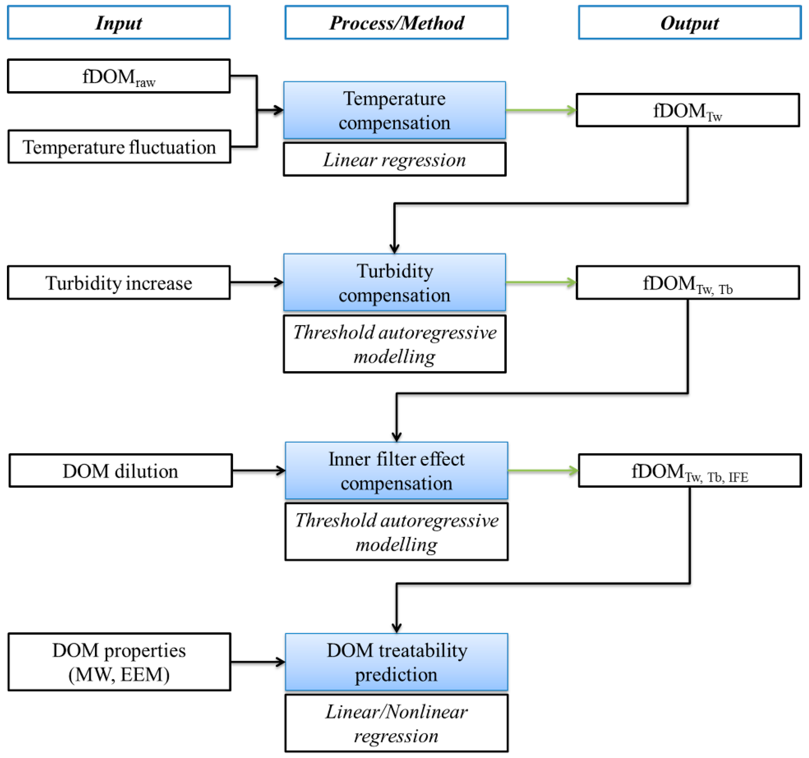
2.5. Data Analysis and Sequential fDOM Compensation Procedure

Exported sonde data, UV absorption spectra data, and DOC test results were compiled together for pre-processing and statistical analysis. Based on data analysis, linear/nonlinear prediction models were developed to separately account for each interference effect. Sequential compensation of interferences on fluorescence intensity is in accordance with fundamental optical theory [30], however multiple regression models were developed to compare the accuracy. Such models were tested on an independent test set of data; given that the coefficient of determination is inappropriate to test nonlinear models [31], with each models’ performance evaluated using the root mean square error (RMSE). Parameters could be isolated or kept constant for investigation and modelling during our laboratory experiments. Figure 1 outlines the developed sequential fDOM compensation method.

2.6. Linking fDOM with DOM Properties: Experiments

Once the sequential fDOM compensation model was completed, the aim was to check whether the compensated readings could be linked to specific properties of the DOM. Hence, a new set of tests and experiments was conducted.

The fDOM readings were compared against fluorescence and absorbance characteristics, as well as MW distributions, of raw water samples from different sources. Four water samples were collected in October 2017 from three South East Queensland reservoirs; i.e., North Pine Dam, Hinze Dam, Tingalpa reservoir—and one South Australian reservoir; i.e., Myponga reservoir. Compared to Tingalpa reservoir, Hinze Dam, and North Pine Dam have lower historical DOC values (3.9 and 5.3 mg/L respectively). SUVA is typically between 2 and 3 L/(mg m) in the Hinze dam, however, after heavy rainfall events the SUVA was as high as 6 L/(mg m), thus changing considerably the DOM background characteristics. Similarly for the North Pine Dam, although being between 2 and 3 L/(mg m) most of the time, SUVA as low as 0.5 and as high as 7.5 were recorded. In contrast, DOC concentrations in the Myponga reservoir reported to be similar between various seasons (typically between 14 mg/L and 16 mg/L). SUVA levels in Myponga reservoir waters were reported to be slightly lower in the dry season [3.15 ± 0.22 L/(mg m)] compared with the wet season [3.36 ± 0.11 L/(mg m)] [32].

For determination of the concentration of DOM measured as DOC and UV absorbance, water samples were passed through 0.45 mm pre-rinsed sterile cellulose membrane filters prior to analyses. DOC concentration was determined using a TOC analyzer (Model 900, Sievers Instruments, Boulder, CO, USA). UV-Visible light absorbance was measured using a spectro-photometer (UV-120, MIOSTECH Pty Ltd, Chatswood, NSW, Australia) for wavelengths from 200 nm to 700 nm, using a quartz cuvette of 1 cm path length. Color in Hazen Units (HU) was determined by absorbance at 456 nm using a 5 cm path length, glass cuvette and a platinum/cobalt standard (50 HU).

Fluorescence excitation-emission matrix (F-EEM) spectra were acquired (Model LS 55, PerkinElmer, Llantrisant, UK) to characterize DOM in terms of humic-like (HA), fulvic-like (FA), Protein1 (P1), Protein2 (P2) and soluble microbial protein (SMP)-like components. A series of emission spectra (280–600 nm) were obtained with 0.5 nm increments over excitation wavelength (200–500 nm) with 5 nm increments. Samples for F-EEM analysis were pre-filtered through 0.45 μm pre-rinsed sterile cellulose membrane filters.

Separation of organic compounds based on apparent MW distributions was performed using high pressure size exclusion chromatography (HPSEC) (Waters 2690 Separation Module and Waters 996 photodiode array detector, Milford, MA, USA) with UV detection at 260 nm wavelength, as described by Chow, et al. [33]. Column size and type, flow rate and other relevant information for the HPSEC-UV detection method have been previously reported [33]. Water samples for HPSEC analysis were passed through 0.22 mm sterile cellulose membrane filters prior to the analysis. Apparent MW distributions of humic-like compounds were measured using HPSEC with fluorescence detection, as described by Aslam, et al. [34]. Excitation and emission wavelengths (320 ex/430 em) were used to investigate the MW distributions of humic-like compounds [35].

PSD in the range of 0.02 to 2000 µm was determined using laser diffraction (Malvern Mastersizer 2000, Malvern Instruments Limited, Malvern, UK). The measurements were conducted using Hydro-G dispersion unit the pump and stirrer speeds set at 1200 rpm and 500 rpm, respectively.

2.7. Linking fDOM with DOM Properties: Data Analysis

All the data from the experiments described above were collected in a .csv format and analyzed through MS Excel. A blank spectrum with high purity Milli-Q water (Merck Millipore, Burlington, MA, USA) was subtracted from the spectra of samples. Raman scans were extracted from blanks and spectra of samples were converted to Raman Units (standard scale). The method of Chen, Westerhoff, Leenheer and Booksh [35] was used in this study to calculate the relative abundance of each organic group (HA-, FA-, P1-, P2- and SMP-like components).

It was critical to process and elaborate the available data by extracting useful summary statistics and indicators that can characterize the sample upon certain criteria in order to compare fDOM readings with DOM character based on such indexes as described in the literature. As such, a number of indexes were calculated as described below. Importantly, in order to extract meaningful correlations with regards to the fDOM ability to identify specific DOM properties, its compensated measurements need to be normalized to draw conclusions on compositional differences independently from DOM concentration. It was decided to use DOC for normalization, since, despite the added uncertainty associated with DOC results, it has been selected for this purpose in several previous studies, as reported in Korak, et al. [36]. Therefore, the normalized fDOM; i.e., fDOM/DOC, will be defined hereafter as nfDOM.

The fluorescence index (FI) was the first calculated indicator, which is defined as the ratio of fluorescence emission intensity at wavelength 450 nm to that at 500 nm, at an excitation wavelength of 370 nm [20]; this was later red-shifted to 470 nm and 520 nm [21]. The lower the FI, the more aromatic the DOM is; the higher the FI, the more microbially dominated the DOM is. Previous studies also found a negative correlation with DOC, with increasing FI for lower DOC levels [36].

Also calculated was the humification index (HIX) as in Zsolnay, Baigar, Jimenez, Steinweg, and Saccomandi [22] and Ohno [23]. HIX is an indicator of the humic substance content or the extent of humification, with higher values indicating an increasing degree of humification. Another considered index was BIX, or the index of recent autochthonous contributions [37]. It is an indicator of autotrophic productivity: high values (>1) correspond to recently produced DOM of autochthonous origin. Finally, the relative fluorescence efficiency (RFE) was calculated, indicating the amount of algal DOM as described in Hansen, Kraus, Pellerin, Fleck, Downing, and Bergamaschi [24].

With regards to the HPSEC results, there have been many suggestions in the literature on how to summarize the resulting MW distributions. Some of the most common metrics have been the weight-averaged MW, the number-average MW, and polydispersivity, as described in Her, et al. [38]. As weight-average MW has been linked to aromaticity before [39,40], which in turn has been linked to DOC removal capacity [25] and to the amount of humics [41], for this study the focus was on this index. In particular, a slightly different formulation is herein proposed, using a logarithmic transformation in order to reduce the influence of extremely high MW compounds, and increase the focus towards the lower range of MW; i.e., where most of the DOM in the analyzed samples is located. The proposed formula is as follows:

$${\mathrm{M}}_{\mathrm{wt}}={10}^{\frac{{{\displaystyle \sum }}_{\mathrm{i}=1}^{\mathrm{n}}{\mathrm{h}}_{\mathrm{i}}·{\log }_{10}{\mathrm{M}}_{\mathrm{i}}}{{{\displaystyle \sum }}_{\mathrm{i}=1}^{\mathrm{n}}{\mathrm{h}}_{\mathrm{i}}}}$$

(1)

where ${\mathrm{M}}_{\mathrm{wt}}$ is the modified weight-average MW, h_i and M_i are respectively the absorbance in arbitrary units, and the molecular weight at fraction i.

In addition, the relative abundance of components with specific MWs was estimated, based on findings from previous studies. For instance, it is known that HMW (>50,000–90,000 Da) peaks are usually proteins and they are generally indicative of freshly introduced organic matter with short residence time [42]. In the smaller range, peaks around 1800 Da are usually associated with humics. Humics can comprise over half the mass of DOC [43] and potentially up to 90% of DOM in some aquatic ecosystems [44]. More specifically, fulvic acids have been associated to MWs in between 1500 Da and 1100 Da [34], and in between 5000 and 1000 Da [45], with humic acids being in smaller MW range (800 Da–600 Da) [34]. Below 680 Da, DOM has been associated with aliphatic OM or protein-like processes [45]. Another critical cut-off has been made at 1000 Da, with DOM < 1000 Da being more readily available to microorganisms [46] and less bioreactive [47]. Finally, cut-offs can be made based on the ability of removing the different components through water treatment processes, in particular coagulation. In previous studies, DOM peaks at 50,000 Da and 1900 Da were easily removed with one alum dose; the peaks at 800 Da and 1200 Da were only partially removed even after several alum treatments; and the DOM fraction with MW lower than 500 Da could not be removed [33,48].

As a result, for each sample the fractions of DOM with MW: (1) >1500 Da; (2) between 500 and 1500 Da; (3) <500 Da; (4) <1000 Da; and (5) <680 Da were calculated, and correlations with EEM results and nfDOM readings were explored. This is particularly interesting and novel since previous studies making use of normalized fluorescence readings (e.g., Saadi, et al. [49]) did not explore correlations with MW distribution.

Traditional indexes such as UV absorbance at different critical wavelengths (254, 365, 456 nm), the total UV absorbance for the full spectrum, and SUVA were also quantified. SUVA also provides an indication of aromaticity [50]; previous studies have found a good link between SUVA and DOC treatability [51] while others did not [25]. This has been explained by the fact that SUVA is an average value, and does not provide information on the underlying distribution; hence that same SUVA value could be the result of a normal distribution, or of a very asymmetric one with large standard deviation and thus with a large proportion of organic matter with low SUVA (i.e., poor treatability) [25]. Regardless, SUVA was considered too for data analysis purposes.

3. Results

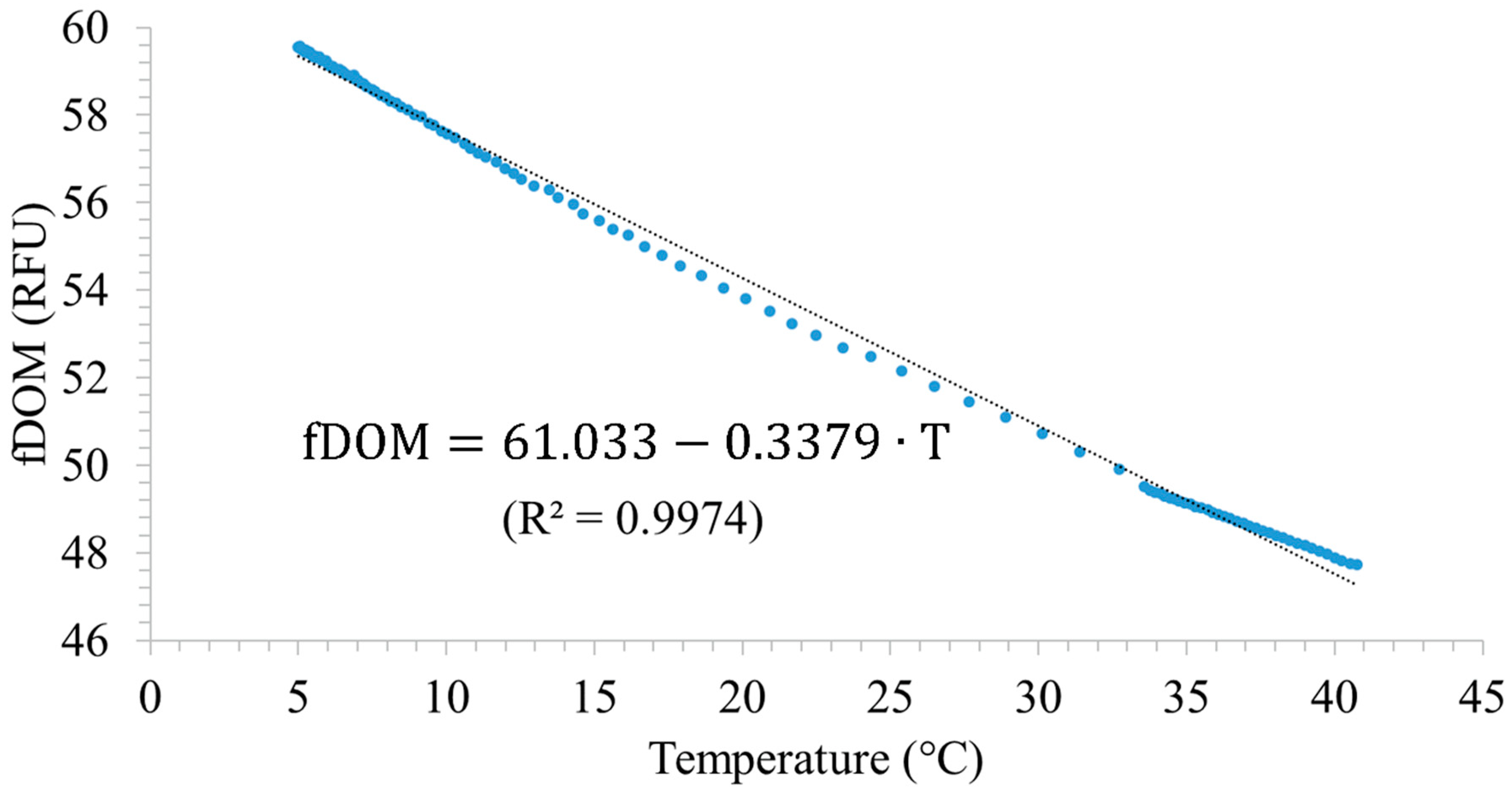
3.1. Temperature Effects on fDOM Measurements

As discussed in previous studies [27], a single DOC concentration should suffice for determination of temperature effects on fDOM measurements. Therefore, in this work the investigation of temperature interference on fDOM readings was performed only using natural raw water collected in April 2017 from Lake Tingalpa at a DOC concentration of 14 mg/L. The linear regression compensation model for temperature over the range 5 to 40 °C (Figure 2) resulted in a near-perfect fit (R² > 0.99), meaning that the fDOM reading can be accurately adjusted to account for temperature values moving away from the reference value.

The compensation equation was developed adapting from Watras, Hanson, Stacy, Morrison, Mather, Hu and Milewski [27], who developed a temperature compensation method for chromophoric dissolved organic matter (CDOM) fluorescence sensors readings based on the following equation: ${\mathrm{CDOM}}_{\mathrm{r}}={\mathrm{CDOM}}_{\mathrm{m}}/\left[1+\mathsf{\rho }\left({\mathrm{T}}_{\mathrm{m}}-{\mathrm{T}}_{\mathrm{r}}\right)\right]$, where T is temperature (°C), $\mathsf{\rho }$ is the temperature coefficient (°C⁻¹), and the subscripts r and m stand for the reference and measured values. ∆fDOM and ∆Temperature were normalized at the fDOM reading corresponding to the temperature of reference i.e., 22.5 °C, as this was the temperature during fDOM calibration with quinine sulphate solution, resulting in the following Equation (2):

$${\mathrm{fDOM}}_{\mathrm{Tw}}={\mathrm{fDOM}}_{\mathrm{m}}/\left[-0.0064\left({\mathrm{T}}_{\mathrm{m}}-{\mathrm{T}}_{\mathrm{r}}\right)+1.009\right]$$

(2)

where T is temperature (°C) and the subscripts T_w and m stand for the temperature-compensated and measured fDOM values, respectively. In order to test this model, Equation (2) was applied to the data collected in March 2017, resulting in a low root mean square error (RMSE) of 0.49 RFU.

A linear and reversible relationship for collisional quenching was expected from a physical point of view [52], since when molecules collide with each other the likelihood of deactivation of an excited-state fluorophore is enhanhced, as long as no thermal degradation occurs. Interestingly, the quenching effect seems to be slightly weaker (0.33%/°C) than what was reported in previous studies [4].

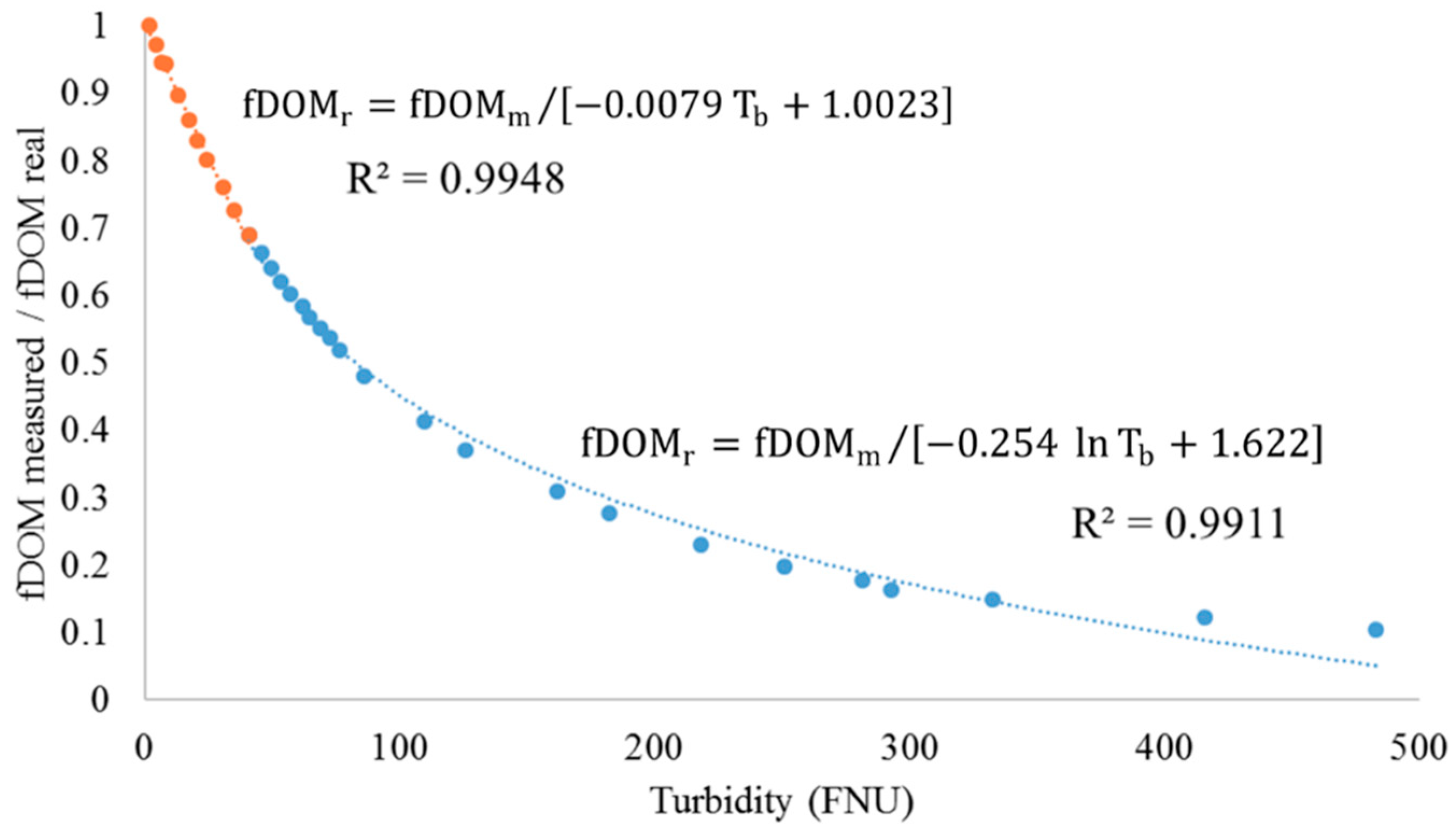
3.2. Turbidity Effects on fDOM Measurements

By plotting fDOM signal against turbidity (Figure 3), it was evident that the fluorescence intensity behavior was linear at the lower end of the turbidity range, and nonlinear after a certain threshold; i.e., 40 FNU. UV₂₅₄ remained relatively constant throughout the experiment, with absorbance values varying from 0.508 to 0.533 cm⁻¹, and DOC was held steady at 14 mg/L. Consequently, in these experiments, after normalization of fDOM the data was fitted with a threshold autoregressive model [53] containing linear and logarithmic terms, based on the systems of Equations (3) and (4):

$${\mathrm{fDOM}}_{\mathrm{Tb}}={\mathrm{fDOM}}_{\mathrm{m}}/\left[-0.0079{\mathrm{T}}_{\mathrm{b}}+1.0023\right];{\mathrm{T}}_{\mathrm{b}}\le 40\mathrm{FNU}$$

(3)

$${\mathrm{fDOM}}_{\mathrm{Tb}}={\mathrm{fDOM}}_{\mathrm{m}}/\left[-0.254\ln {\mathrm{T}}_{\mathrm{b}}+1.622\right];{\mathrm{T}}_{\mathrm{b}}>40\mathrm{FNU}$$

(4)

where T_b is turbidity in FNU, and the subscripts T_b and m relate to the turbidity-compensated and measured fDOM values, respectively. Data acquired in May 2017 was used for testing, resulting in a low RMSE of 0.21 RFU. Future work will examine the suitability of equations for different seasons and extreme weather events, as characteristics of suspended solids (algae, sand, silt, clay etc.) may vary with time, altering the fDOM signal bias.

In subsequent experiments with raw waters from four different sources, it was observed that the quenching effect by turbidity varied, expectedly, based on turbidity type. By measuring fDOM and turbidity before and after sample filtration, and by back-calculating the loss in fDOM signal per NTU of turbidity added, it was noticed that the Capalaba sample presented the highest loss in fDOM signal (3.43% per FNU of turbidity added), while North Pine the lowest (1.04%); both Hinze (2.96%) and Myponga (2.39%) had mid-range interferences. Looking at Figure 4, Capalaba has the highest abundance of smaller particles, while North Pine has the largest particles. This is important since, the way turbidity is measured, particles of different sizes contribute differently to turbidity [54]; hence a measurement of 1 FNU in Capalaba is different from 1 FNU in North Pine. This can be explained by the characteristic that 1 FNU made of smaller particles has a higher probability of fluorescence interference on fDOM. As a consequence, there is a clear link between the particle size of the suspended sediments, turbidity, and fDOM signal loss, similarly to the findings of recent studies [11]; hence there is potential, in the future, to develop a more general model capable to automatically recalibrate Equations (3) and (4) based on the PSD of suspended solids in a new location.

3.3. Inner Filter Effect on fDOM Measurements

Each water body is likely to have a specific threshold where the concentration of its particular DOM interferes with fDOM linearity. As UV₂₅₄ is known to be a good proxy for DOC concentration, it was used for IFE estimation, instead of the absorbance at the excitation/emission wavelength 365 nm/480 nm. Figure 5 illustrates the UV₂₅₄ threshold beyond which fDOM signal is underestimated due to optical density increase.

According to these findings, fDOM readings in this natural water only need to be compensated when UV₂₅₄ is over 0.6 cm⁻¹. Equation (5) provides a IFE compensation model that considers the behavior of fDOM beyond this threshold by quantifying the gap between the expected fDOM readings assuming no IFE (i.e., applying the linear equation at low UV₂₅₄) and the actual, lower fDOM reading resulting from IFE (i.e., applying the nonlinear equation at high UV₂₅₄).

$${\mathrm{fDOM}}_{\mathrm{IFE}}={\mathrm{fDOM}}_{\mathrm{m}}/\left[1.1717{\mathrm{e}}^{-0.315{\mathrm{UV}}_{254}}\right];{\mathrm{UV}}_{254}\ge 0.6{\mathrm{cm}}^{-1}$$

(5)

where UV₂₅₄ is UV absorbance at 254 nm in cm⁻¹, and the subscripts IFE and m refer to the IFE-compensated and measured fDOM values, respectively.

In Figure 6, IFE results are reported for three different reservoirs tested in this study, namely North Pine (NP), Hinze dam (HD), and Capalaba (CAP-as per Figure 5). Interestingly, IFE has similar quenching magnitude for the three different reservoirs for UV₂₅₄ below approximately 1.2 cm⁻¹. However, for very elevated DOM concentrations, different patterns emerged, with DOM from Capalaba causing lower self-quenching than DOM from NP and HD. These differences can be due to different DOM properties such as different fluorophores and fluorescence quantum yield in each reservoir. In Downing, Pellerin, Bergamaschi, Saraceno, and Kraus [12], although two different standard DOM were tested for IFE, no significant differences were noticed/discussed. In addition, the absorbance range analyzed was much narrower, potentially not including DOM concentrations high enough to notice remarkable discrepancies. However, for the range of DOM concentrations typically recorded at these three locations, DOM properties do not seem to affect IFE and thus the same compensation equation could be used for these three different reservoirs.

3.4. Sequential Model Validation

A training and test set of data was created by dividing the database built over time with the results of the experiments using a 70/30 ratio, i.e., the training set accounted for 70% of the full dataset and the test set for the remaining 30%. The fully compensated fDOM readings; i.e., after sequentially applying Equations (2)–(5)—were compared against the expected fDOM readings; i.e., those recorded during the same experiments but with minimum interferences before; e.g., changing temperature, or the increasing turbidity or DOM. For comparison purposes, a linear and a non-linear multivariate model were also developed to challenge the assumption that accounting for each effect separately, and cumulatively, would yield better results. The performance of the models on the test set was found to be:

• RMSE = 3.38 RFU for the linear multivariate model,
• RMSE = 2.73 RFU for the non-linear multivariate model, and
• RMSE = 0.57 RFU for the sequential model

The sequential fDOM compensation model had a significantly lower RMSE than the multivariate ones and was selected for fDOM compensation. This was expected since fundamental optical theory holds that quenching effects are simply additive and can be approached separately [30].

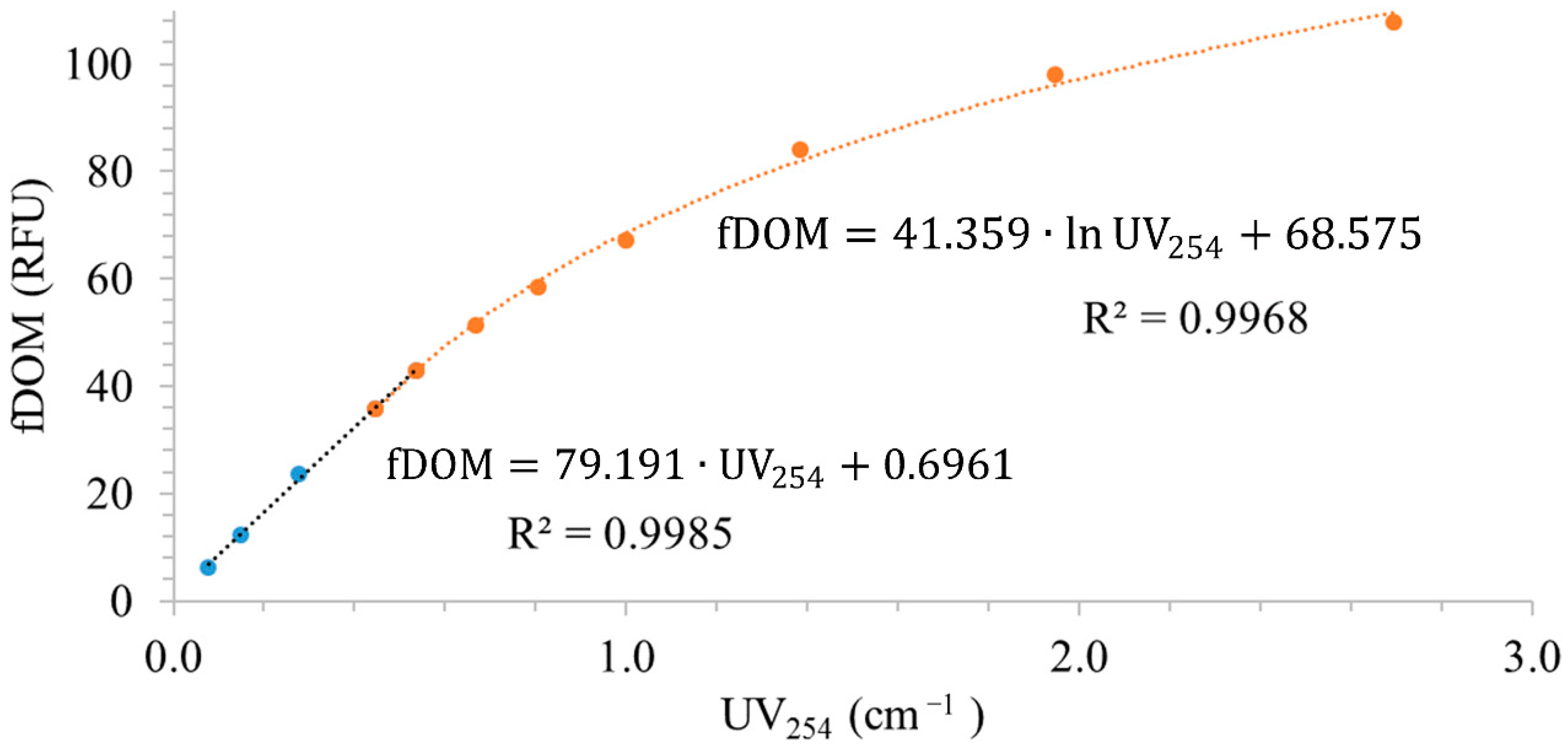
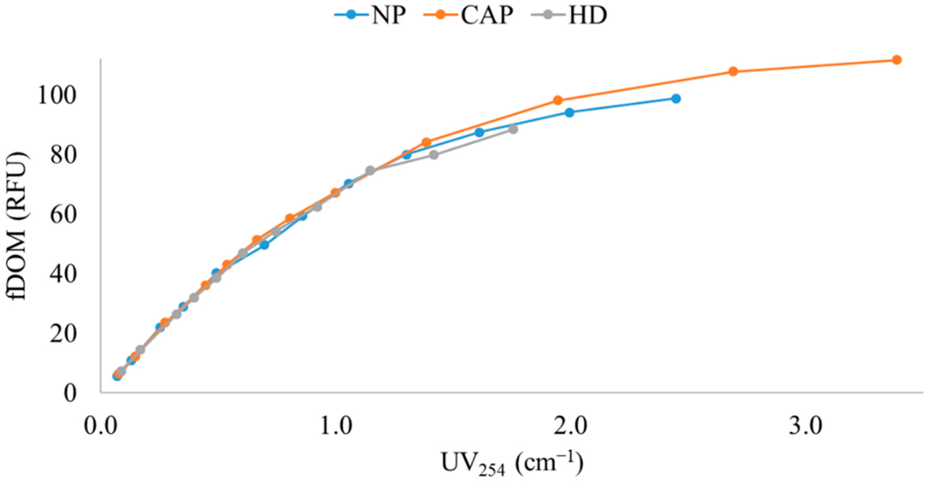
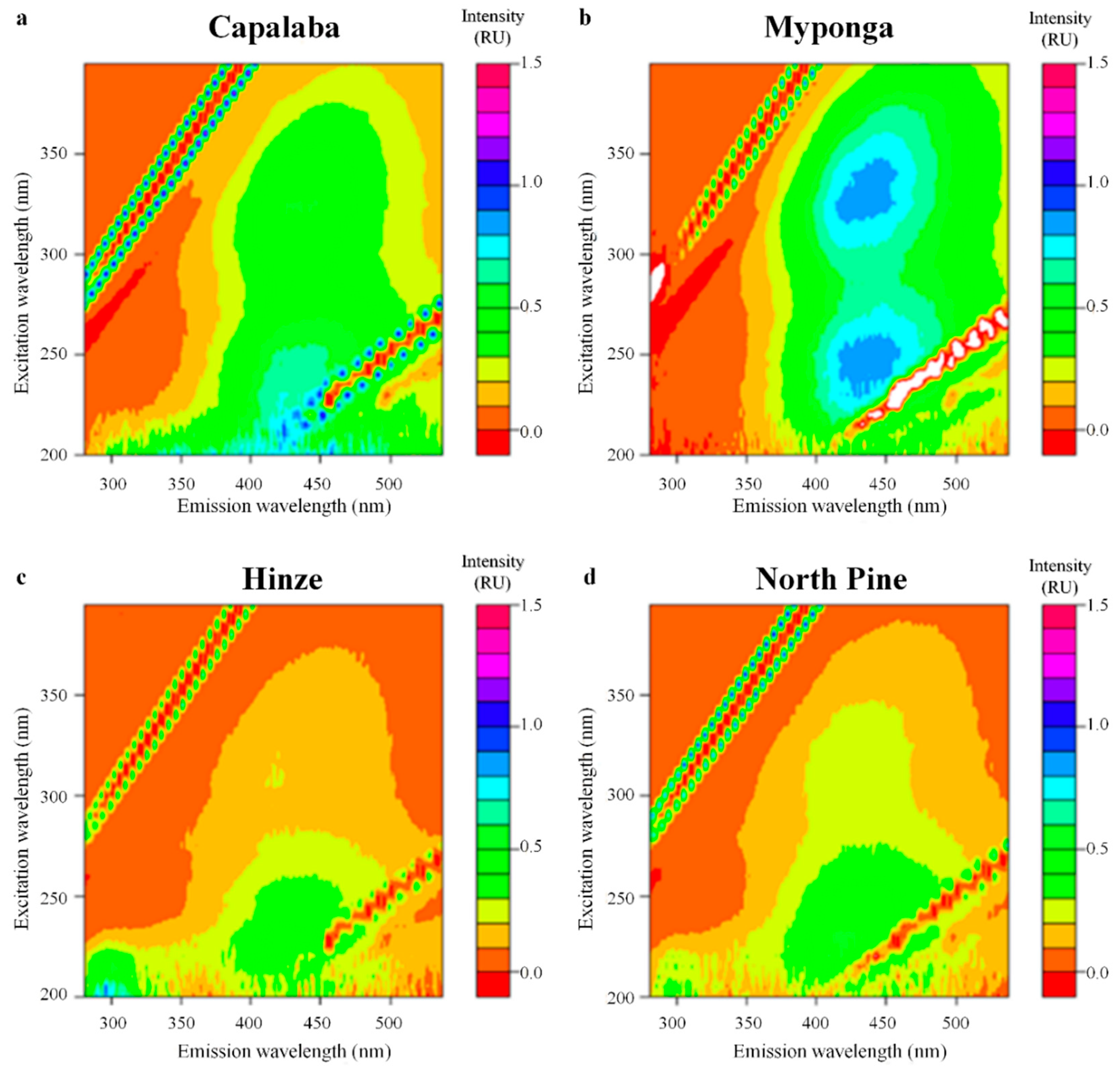
3.5. EEM vs. fDOM Signal

Figure 7 presents the optical maps in which different fractions of DOM are characterized according to their fluorescent properties for the four different reservoirs. The Myponga reservoir has the strongest fluorescence intensity in the regions III and V, as well as the highest DOC (15 mg/L), however it has the weakest signal in the other regions. Capalaba has its strongest fluorescence signal in region III, followed by region V, but also shows some intensity in regions I and II. The other two waters have low florescence in regions V and III, but stronger signals in region I, especially Hinze.

Fluorescence spectroscopy analysis helped calculate the relative abundances of each of the five different fractions of DOM as defined by Chen, Westerhoff, Leenheer, and Booksh [35] and compared them against the fDOM signal, UV₂₅₄ and UV₄₅₆ as to investigate direct correlations (Figure 8).

Table 1. Coefficients of determination for analyzed variables—EEM.

Parameter	P1	P2	SMP	FA	HA	DOC	UV254	fDOM	tot Spectrum abs	SUVA	fDOM/DOC
P1		0.23	0.94	0.77	0.98	0.86	0.82	0.98	0.83	0.60	0.94
P2	0.23		0.42	0.70	0.35	0.60	0.61	0.36	0.61	0.74	0.08
SMP	0.94	0.42		0.89	0.96	0.94	0.88	0.96	0.89	0.57	0.77
FA	0.77	0.70	0.89		0.87	0.99	0.98	0.88	0.99	0.85	0.58
HA	0.98	0.35	0.96	0.87		0.94	0.92	0.99	0.92	0.64	0.88
DOC	0.86	0.60	0.94	0.99	0.94		0.99	0.94	0.99	0.80	0.68
UV254	0.82	0.61	0.88	0.98	0.92	0.99		0.92	0.99	0.87	0.66
fDOM	0.98	0.36	0.96	0.88	0.99	0.94	0.92		0.93	0.65	0.87
tot spectrum abs	0.83	0.61	0.89	0.99	0.92	0.99	0.99	0.93		0.09	0.76
SUVA	0.60	0.74	0.57	0.85	0.64	0.80	0.87	0.65	0.09		0.38
fDOM/DOC	0.94	0.08	0.78	0.58	0.88	0.68	0.66	0.87	0.76	0.38

Green = higher correlation; red = lower correlation.

also summarizes the correlations among all the variables analyzed (excluding MW-related ones, discussed later).

Firstly, a main peak was observed in the FA region, around an excitation wavelength of 240 nm and an emission wavelength of 440 nm for all the waters, with Myponga having a second peak in the HA region too. As a result, with the exception of Myponga, the predominant DOM fraction is FA for all the samples. FA has the highest specific intensities in the humic-like regions, while HA has the lowest [36]. Also, there are negligible peaks in the protein regions (I and II). This is in line with previous studies for one of the same locations (i.e., Capalaba) where fluorescence in the humic like region was reported as being 7 times higher than in the protein region [25].

It was evident that there was a strong correlation of HA with fDOM (R² = 0.995, p-value < 0.0001) and UV₂₅₄ (R² = 0.92, p-value < 0.05) values in all these four waters, which corroborates with the idea of fDOM being an appropriate tool to measure the fluorescence of a determined concentration of HA in a given sample, as the specific E_x/E_m wavelength pair seems to be representative of the whole Region V. The fDOM readings can be considered compensated, due to tests conducted at ambient temperature, relatively low UV₂₅₄, with filtered samples (i.e., no or low turbidity). However, if the same correlations are analyzed when using raw readings, taken with a certain level (between 1 and 9 FNU) of turbidity, then these correlations slightly drop (R² = 0.992 for HA and 0.88 for UV₂₅₄). An apparent strong correlation (R² = 0.88) seems to be present between fDOM readings and FA too. However, this is a spurious correlation, given that much of the fluorescence picked by the fDOM can be defined as “background fluorescence” due to the FA peak. This can be defined as a limitation of fluorescence regional integration methods. For instance, fluorophores in different regions are related as they have a single emission wavelength but multiple excitation wavelengths [55], thus supporting the hypothesis that a change in fluorescence quantum yield affects the fluorescence simultaneously across different regions [36]. In addition, Korak, Dotson, Summers, and Rosario-Ortiz [36] noticed how the maximum fluorescence intensities of user-defined non-dominant regions lie along the boundary with the dominant region; thus, proving a heavy influence from that dominant region. Therefore in general, with fluorescence regional integration, user-defined regions are heavily influenced by the presence of dominant neighboring fluorophores [36]; as a consequence, the fluorescence picked by the fDOM probe at a specific point in the HA region, would be due to FA or other peaks in neighboring regions; if a peak in a HA region is not present. Accordingly, a good correlation could be found between fDOM and FA only by excluding Myponga, which has a peak in HA too. That said, if the DOM matrix for a certain reservoir (e.g., prevalence of FA, limited HA) is known and constant over seasons, it would be possible to build a model correlating fDOM readings and the abundance of the predominant fraction.

The strong correlation between fDOM and DOC, as well as with UV₂₅₄, serves as a support of the hypothesis that fDOM alone does not provide any insight on the DOM properties, since it is instead linked to the total amount of DOM, which affects its readings even if the peaks are located in other regions. As a consequence, it is much more appropriate, as previously mentioned, to normalize fDOM and consider correlations against fDOM divided by DOC. It can be noticed how the correlation with FA drops to R² = 0.58. The correlations with other indexes reflecting the overall amount of DOM also decrease, since nfDOM provides more specific information about the DOM character, in particular the HA region. Interestingly, although SUVA also relates to aromaticity and humics, it was found to be poorly correlated (R² = 0.38) to nfDOM. No significant correlations were found between nfDOM and the proposed FI, HIX, and BIX.

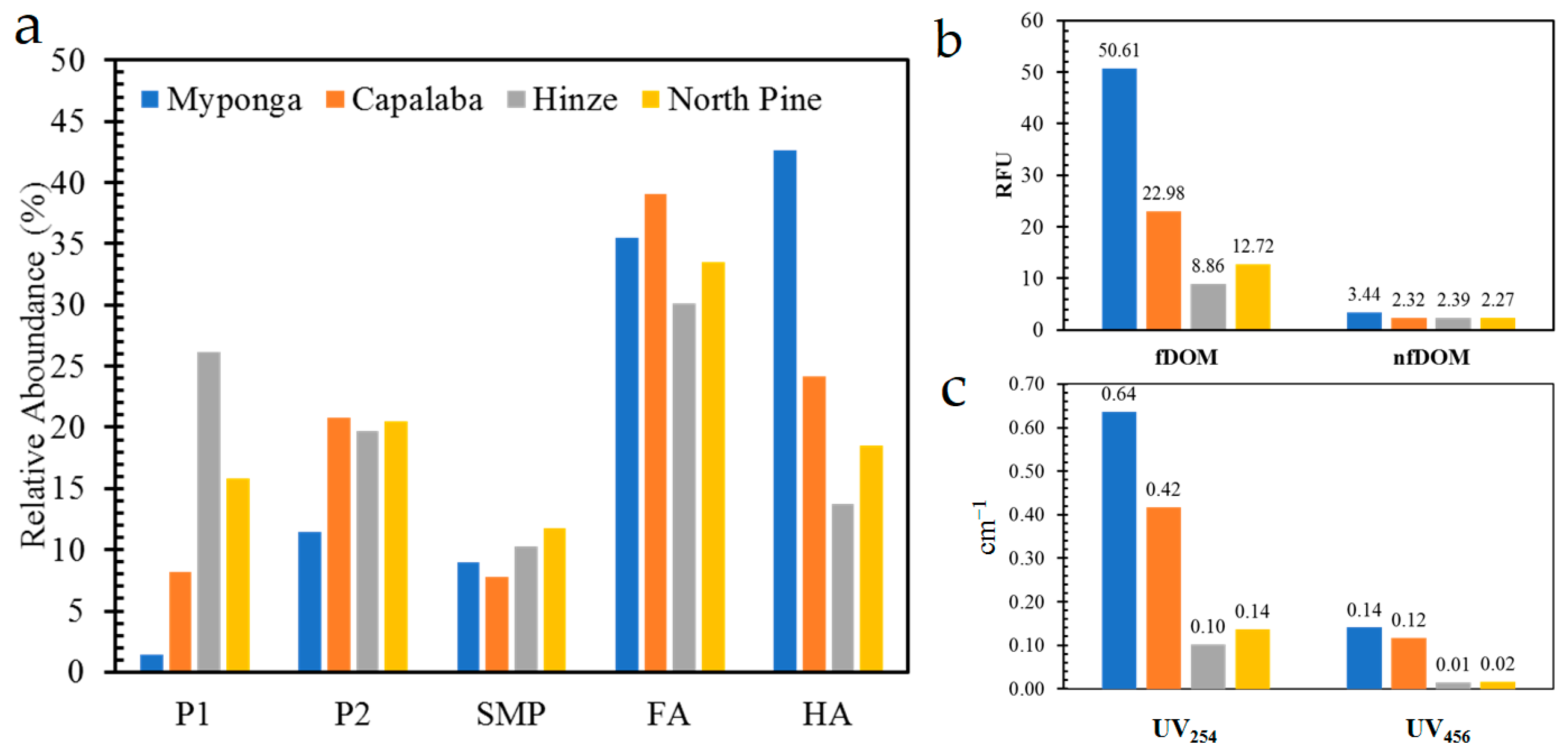
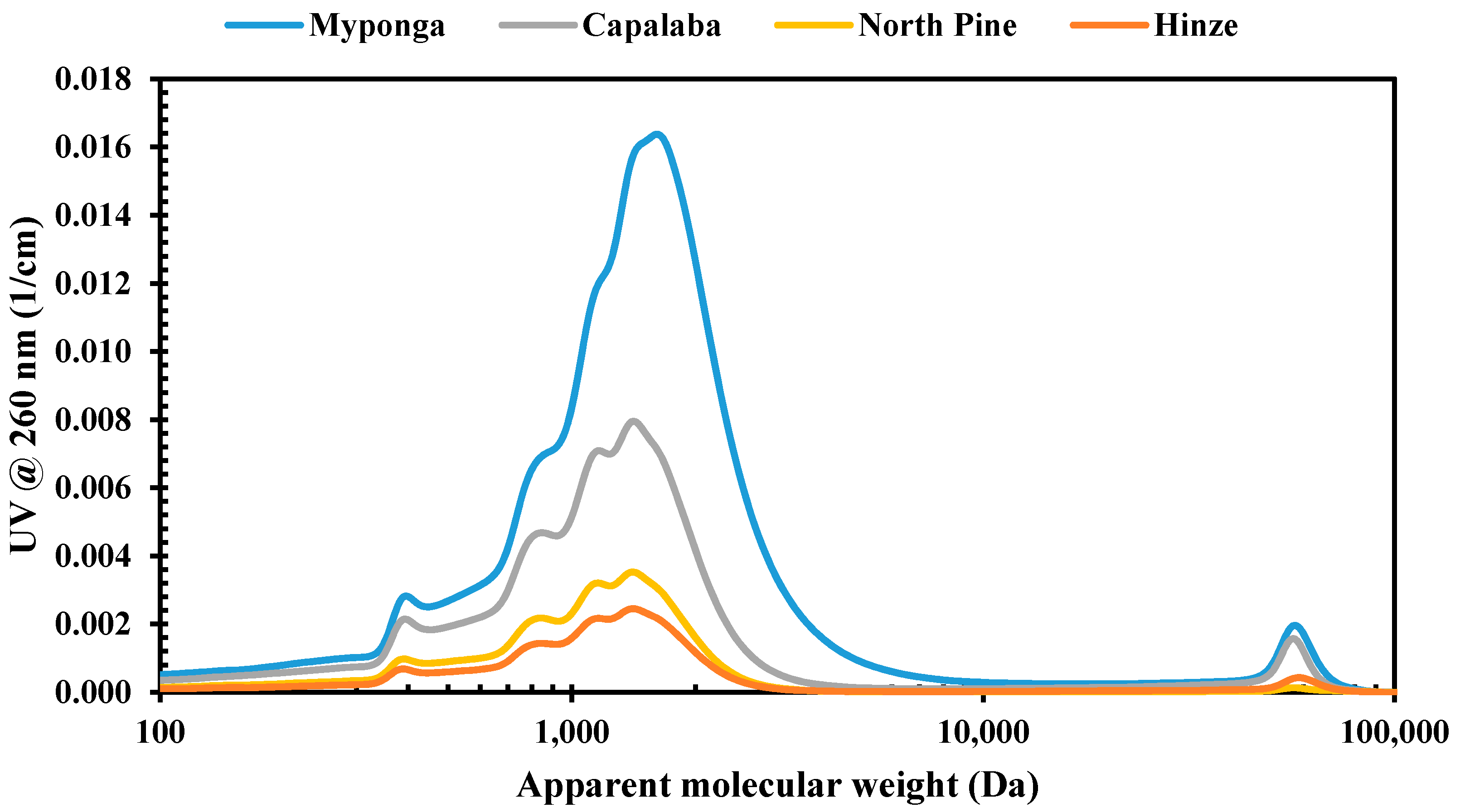
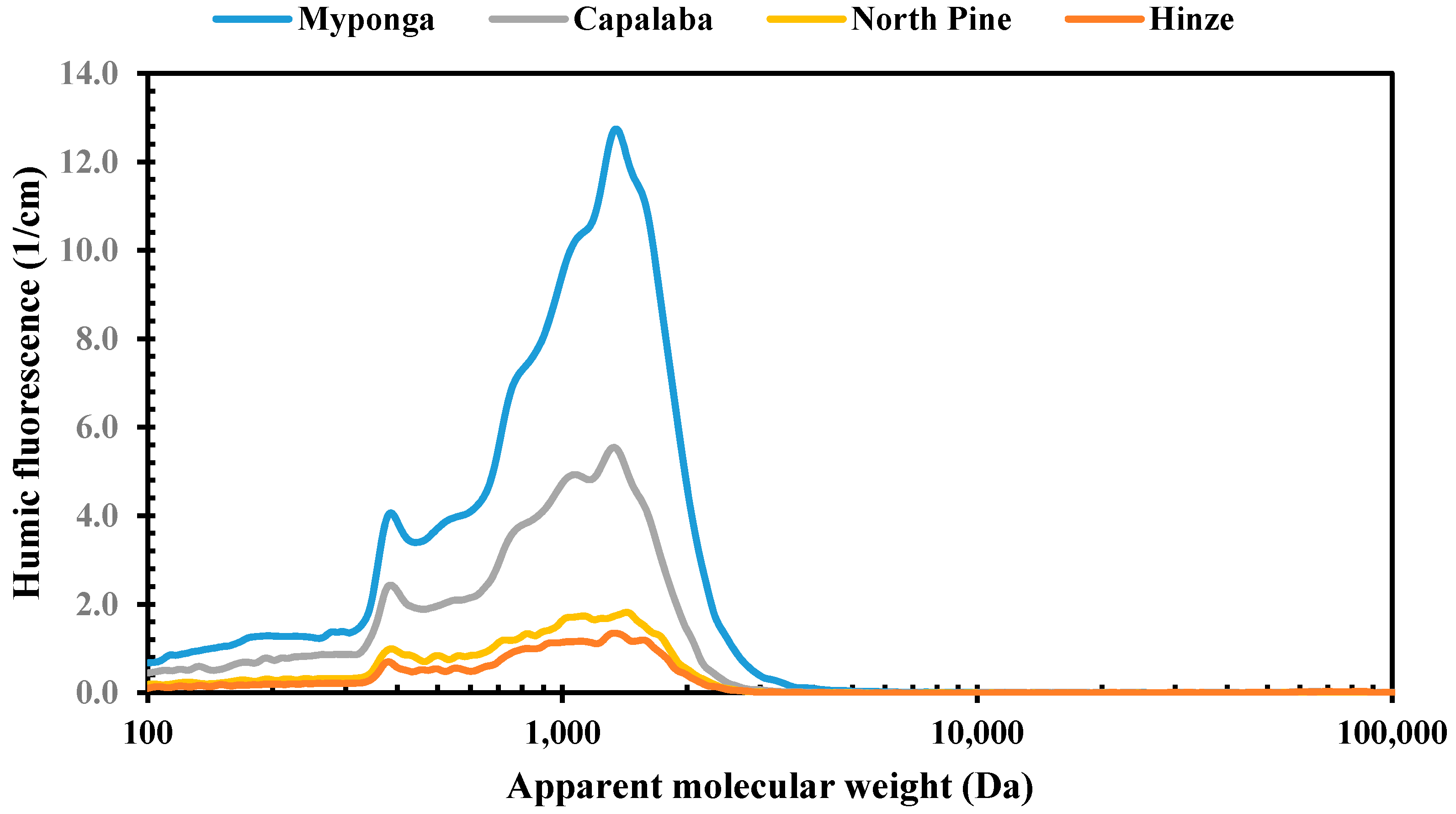
3.6. Molecular Weight vs. fDOM Signal

Table 2. Coefficients of determination between proposed indices and molecular weight (MW) fractions.

Parameter	>1500 Da	500 Da–1500 Da	<500 Da	<1000 Da	<680 Da	Mwt-UV
DOC	0.857	0.9142	0.7223	0.8266	0.8167	0.8057
UV254	0.8694	0.9531	0.71	0.8342	0.8219	0.874
fDOM	0.9588	0.9263	0.9001	0.9498	0.9468	0.8305
tot spectrum abs	0.584	0.4052	0.7344	0.6292	0.6427	0.4501
SUVA	0.6463	0.8343	0.4271	0.5946	0.5757	0.8309
fDOM/DOC	0.9279	0.7789	0.9975	0.9529	0.9607	0.7334

Green = higher correlation; red = lower correlation.

provides the strength of the relationship between nfDOM, fDOM, DOC, UV₂₅₄, and different fractions of DOM based on MW. Figure 9 and Figure 10 also show the absorbance at different MWs for the 4 samples as well as the humics’ fluorescence for the four samples, respectively. The fluorescence of humics is highest at high (>1 KDa) MW, which is in line with the findings of Cuss and Guéguen [56]. The results for fluorescence-protein compounds were below the detection limit of 1 fluorescence unit/cm.

The bulk of the DOM had a MW between 500 Da and 1500 Da, thus overall indexes such as DOC, UV₂₅₄ and to some extent (for the reasons explained above) fDOM showed a good correlation (R² > 0.9, p-value < 0.05) with this MW fraction. A quite strong (0.8 < R² < 0.9) correlation was also found between those indexes, including SUVA, and the overall ${\mathrm{M}}_{\mathrm{wt}}$. This is because indexes such as SUVA are linked to the abundance of the aromatic fraction, which typically has a larger MW [40]. A strong negative correlation between the indexes, fDOM and ${\mathrm{M}}_{\mathrm{wt}}$ of the humics fraction, was noticed; this is in line with previous research [57] noticing higher fluorescence intensities with decreasing MW. What can be noticed though, is the strong, negative, correlation between nfDOM, and LMW fractions of the DOM. In particular, there was almost a perfect fit (R² = 0.99, p-value $\cong$ 0.001) between nfDOM and DOM with MW lower than 500 Da, i.e., the fraction extremely recalcitrant to coagulation [33] and thus of more interest to DWTP operators. In contrast, SUVA, which has been used in the past as a way to also quantify the treatability of the water, does not show any significant correlation with any of the MW fractions.

4. Discussion

Although further validation is needed to confirm the above correlations, it is argued that there is potential to use nfDOM as a substitute for SUVA, which can provide more useful insights on DOM character and treatability. Given that online DOC sensors have recently been developed, such indexes could be estimated continuously, in near real-time, either at the drinking water treatment plant or for a vertical profile at a reservoir. Additionally, if these same correlations are estimated when only using raw fDOM readings, their prediction reliability drops from R² = 0.99 to R² = 0.90, thus demonstrating the importance of compensating fDOM readings using the method proposed herein.

As mentioned previously, several studies have been conducted to analyze fluorescence quenching effects; also, studies exist that explored linking a specific wavelength pair of the excitation emission spectrum to DOM treatability (e.g., Shutova, Baker, Bridgeman and Henderson [25]). However, to the authors’ knowledge, this is the first study providing a comprehensive methodological framework to fully, and accurately, compensate the readings of an existing, commercially available fDOM probe, based on universal as well as site-specific parameters, and to use such readings to provide information on the abundance of critical molecular weight fractions of DOM. As such, future work will seek to further validate such findings, and make a case for moving away from time-consuming SUVA estimations in favor of a real-time monitoring of DOM properties through compensated fDOM probes’ readings. Importantly, if the fDOM probe is installed in a lake or reservoir on a vertical profiling system, such DOM properties will be estimated at high temporal (e.g., hourly) and spatial vertical (e.g., every meter) resolution, allowing for a unique, comprehensive understanding of variations of DOM composition under different environmental conditions (including, for instance, immediately following a heavy rainfall event). A further significant implication of the research outcome is that, by better monitoring the DOM properties of the incoming raw water, drinking water treatment plant operators would be able to not only maximize DOM removal, but also in turn minimize the formation of potentially carcinogenic disinfection byproducts, thus effectively reducing health risks for the drinking water consumers.

5. Conclusions

A sequential compensation method to account for in situ interferences (i.e., temperature, turbidity, inner filter effect) on measurements of a fDOM probe has been developed, based on raw water sampled from a South-East Queensland reservoir and data collected during laboratory experiments. Temperature had a linear, inverse relationship with fDOM, whereas the turbidity effect on fDOM was best described by a threshold autoregressive model. An inner filtering effect played a role in self-quenching fDOM at UV₂₅₄ levels above 0.6 cm⁻¹. The sequential model yielded a higher accuracy than other developed multivariate regression models. The compensation framework relies on site-specific water quality rather than standards and it can be straightforwardly re-applied to other sites where the same probe is deployed.

The compensated fDOM readings were used to determine correlations between fDOM and DOM properties. Although working at a specific wavelength contained in the humic-like region, it was found that fDOM does not directly provide any specific insights on the DOM character as it is affected by peaks in neighboring domain regions of the fluorescence excitation-emission matrix, and it is thus related to the total amount of DOM present. However, a strong correlation was found between a normalized fDOM index (i.e., fDOM/DOC) and the low molecular weight fraction (<500 Da) of DOM, which is typically regarded as recalcitrant to removal with conventional coagulation processes. The correlation coefficient decreased by more than 10%, if raw instead of compensated fDOM readings were used.

The findings demonstrate the potential to use compensated and normalized fDOM values in place of SUVA in order to more effectively inform the drinking water treatment plant on DOM-related incoming raw water quality risks associated with the low molecular weight fraction. This information can assist drinking water treatment plant operators to optimize the coagulation process and DOM removal, which would reduce the health risks associated with excessive disinfection byproduct formation in the water distribution system.

References

1. Zhao, Z.-Y.; Gu, J.-D.; Li, H.-B.; Li, X.-Y.; Leung, K.M.-Y. Disinfection characteristics of the dissolved organic fractions at several stages of a conventional drinking water treatment plant in southern China. J. Hazard. Mater. 2009, 172, 1093–1099. [Google Scholar] [CrossRef] [PubMed]
2. Kim, H.-C.; Lee, W.M.; Lee, S.; Choi, J.; Maeng, S.K. Characterization of organic precursors in DBP formation and AOC in urban surface water and their fate during managed aquifer recharge. Water Res. 2017, 123, 75–85. [Google Scholar] [CrossRef] [PubMed]
3. Sharp, E.L.; Jarvis, P.; Parsons, S.A.; Jefferson, B. Impact of fractional character on the coagulation of nom. Colloids Surf. A 2006, 286, 104–111. [Google Scholar] [CrossRef]
4. Henderson, R.K.; Baker, A.; Murphy, K.R.; Hambly, A.; Stuetz, R.M.; Khan, S.J. Fluorescence as a potential monitoring tool for recycled water systems: A review. Water Res. 2009, 43, 863–881. [Google Scholar] [CrossRef] [PubMed]
5. Bertone, E.; Stewart, R.A.; Zhang, H.; Bartkow, M.; Hacker, C. An autonomous decision support system for manganese forecasting in subtropical water reservoirs. Environ. Model. Softw. 2015, 73, 133–147. [Google Scholar] [CrossRef]
6. Bertone, E.; Stewart, R.A.; Zhang, H.; Veal, C. Data-driven recursive input–output multivariate statistical forecasting model: Case of do concentration prediction in Advancetown Lake, Australia. J. Hydroinf. 2015, 17, 817–833. [Google Scholar] [CrossRef]
7. Carstea, E.M. Fluorescence spectroscopy as a potential tool for in-situ monitoring of dissolved organic matter in surface water systems. In Water Pollution; INTECH Open Access Publisher: London, UK, 2012. [Google Scholar]
8. Piana, M.J.; Zahir, K.O. Investigation of metal ions binding of humic substances using fluorescence emission and synchronous-scan spectroscopy. J. Environ. Sci. Health Part B 2000, 35, 87–102. [Google Scholar] [CrossRef]
9. Hudson, N.; Baker, A.; Reynolds, D. Fluorescence analysis of dissolved organic matter in natural, waste and polluted waters—A review. River Res. Appl. 2007, 23, 631–649. [Google Scholar] [CrossRef]
10. Spencer, R.G.M.; Bolton, L.; Baker, A. Freeze/thaw and pH effects on freshwater dissolved organic matter fluorescence and absorbance properties from a number of UK locations. Water Res. 2007, 41, 2941–2950. [Google Scholar] [CrossRef] [PubMed]
11. Saraceno, J.F.; Shanley, J.B.; Downing, B.D.; Pellerin, B.A. Clearing the waters: Evaluating the need for site-specific field fluorescence corrections based on turbidity measurements. Limnol. Oceanogr. Methods 2017. [Google Scholar] [CrossRef]
12. Downing, B.D.; Pellerin, B.A.; Bergamaschi, B.A.; Saraceno, J.F.; Kraus, T.E.C. Seeing the light: The effects of particles, dissolved materials, and temperature on in situ measurements of DOM fluorescence in rivers and streams. Limnol. Oceanogr. Methods 2012, 10, 767–775. [Google Scholar] [CrossRef] [Green Version]
13. Wang, T.; Zeng, L.-H.; Li, D.-L. A review on the methods for correcting the fluorescence inner-filter effect of fluorescence spectrum. Appl. Spectrosc. Rev. 2017, 52, 883–908. [Google Scholar] [CrossRef]
14. Baker, A. Thermal fluorescence quenching properties of dissolved organic matter. Water Res. 2005, 39, 4405–4412. [Google Scholar] [CrossRef] [PubMed]
15. Carstea, E.M.; Baker, A.; Bieroza, M.; Reynolds, D.M.; Bridgeman, J. Characterisation of dissolved organic matter fluorescence properties by parafac analysis and thermal quenching. Water Res. 2014, 61, 152–161. [Google Scholar] [CrossRef] [PubMed]
16. Coble, P.G.; Lead, J.; Baker, A.; Reynolds, D.M.; Spencer, R.G. Aquatic Organic Matter Fluorescence; Cambridge University Press: New York, NY, USA, 2014. [Google Scholar]
17. Khamis, K.; Sorensen, J.; Bradley, C.; Hannah, D.; Lapworth, D.; Stevens, R. In situ tryptophan-like fluorometers: Assessing turbidity and temperature effects for freshwater applications. Environ. Sci. Process. Impacts 2015, 17, 740–752. [Google Scholar] [CrossRef] [PubMed] [Green Version]
18. Khamis, K.; Bradley, C.; Stevens, R.; Hannah, D.M. Continuous field estimation of dissolved organic carbon concentration and biochemical oxygen demand using dual-wavelength fluorescence, turbidity and temperature. Hydrol. Process. 2017, 31, 540–555. [Google Scholar] [CrossRef]
19. Shutova, Y.; Baker, A.; Bridgeman, J.; Henderson, R. On-line monitoring of organic matter concentrations and character in drinking water treatment systems using fluorescence spectroscopy. Environ. Sci. Water Res. Technol. 2016, 2, 749–760. [Google Scholar] [CrossRef]
20. McKnight, D.M.; Boyer, E.W.; Westerhoff, P.K.; Doran, P.T.; Kulbe, T.; Andersen, D.T. Spectrofluorometric characterization of dissolved organic matter for indication of precursor organic material and aromaticity. Limnol. Oceanogr. 2001, 46, 38–48. [Google Scholar] [CrossRef] [Green Version]
21. Cory, R.M.; Miller, M.P.; McKnight, D.M.; Guerard, J.J.; Miller, P.L. Effect of instrument-specific response on the analysis of fulvic acid fluorescence spectra. Limnol. Oceanogr. Methods. 2010, 8, 67–78. [Google Scholar] [Green Version]
22. Zsolnay, A.; Baigar, E.; Jimenez, M.; Steinweg, B.; Saccomandi, F. Differentiating with fluorescence spectroscopy the sources of dissolved organic matter in soils subjected to drying. Chemosphere 1999, 38, 45–50. [Google Scholar] [CrossRef]
23. Ohno, T. Fluorescence inner-filtering correction for determining the humification index of dissolved organic matter. Environ. Sci. Technol. 2002, 36, 742–746. [Google Scholar] [CrossRef] [PubMed]
24. Hansen, A.M.; Kraus, T.E.; Pellerin, B.A.; Fleck, J.A.; Downing, B.D.; Bergamaschi, B.A. Optical properties of dissolved organic matter (DOM): Effects of biological and photolytic degradation. Limnol. Oceanogr. 2016, 61, 1015–1032. [Google Scholar] [CrossRef] [Green Version]
25. Shutova, Y.; Baker, A.; Bridgeman, J.; Henderson, R.K. Spectroscopic characterisation of dissolved organic matter changes in drinking water treatment: From parafac analysis to online monitoring wavelengths. Water Res. 2014, 54, 159–169. [Google Scholar] [CrossRef] [PubMed]
26. Peleato, N.M.; Andrews, R.C. Comparison of three-dimensional fluorescence analysis methods for predicting formation of trihalomethanes and haloacetic acids. J. Environ. Sci. 2015, 27, 159–167. [Google Scholar] [CrossRef] [PubMed]
27. Watras, C.J.; Hanson, P.C.; Stacy, T.L.; Morrison, K.M.; Mather, J.; Hu, Y.H.; Milewski, P. A temperature compensation method for cdom fluorescence sensors in freshwater. Limnol. Oceanogr. Method. 2011, 9, 296–301. [Google Scholar] [CrossRef]
28. Lee, E.-J.; Yoo, G.-Y.; Jeong, Y.; Kim, K.-U.; Park, J.-H.; Oh, N.-H. Comparison of UV–VIS and fdom sensors for in situ monitoring of stream doc concentrations. Biogeosciences 2015, 12, 3109–3118. [Google Scholar] [CrossRef]
29. Serkiz, S.M.; Perdue, E.M. Isolation of dissolved organic matter from the Suwannee River using reverse osmosis. Water Res. 1990, 24, 911–916. [Google Scholar] [CrossRef]
30. Lakowicz, J.R. Principles of Fluorescence Spectroscopy, 3rd ed.; Springer: Berlin, Germany, 2006. [Google Scholar]
31. Spiess, A.-N.; Neumeyer, N. An evaluation of R2 as an inadequate measure for nonlinear models in pharmacological and biochemical research: A Monte Carlo approach. BMC Pharmacol. 2010, 10, 6. [Google Scholar] [CrossRef] [PubMed]
32. Awad, J.; van Leeuwen, J.; Chow, C.W.; Smernik, R.J.; Anderson, S.J.; Cox, J.W. Seasonal variation in the nature of DOM in a river and drinking water reservoir of a closed catchment. Environ. Pollut. 2017, 220, 788–796. [Google Scholar] [CrossRef] [PubMed]
33. Chow, C.W.; Fabris, R.; Leeuwen, J.v.; Wang, D.; Drikas, M. Assessing natural organic matter treatability using high performance size exclusion chromatography. Environ. Sci. Technol. 2008, 42, 6683–6689. [Google Scholar] [CrossRef] [PubMed]
34. Aslam, Z.; Chow, C.W.K.; Murshed, F.; van Leeuwen, J.A.; Drikas, M.; Wang, D. Variation in character and treatability of organics in river water: An assessment by HPAC and alum coagulation. Sep. Purif. Technol. 2013, 120, 162–171. [Google Scholar] [CrossRef]
35. Chen, W.; Westerhoff, P.; Leenheer, J.A.; Booksh, K. Fluorescence excitation-emission matrix regional integration to quantify spectra for dissolved organic matter. Environ. Sci. Technol. 2003, 37, 5701–5710. [Google Scholar] [CrossRef] [PubMed]
36. Korak, J.A.; Dotson, A.D.; Summers, R.S.; Rosario-Ortiz, F.L. Critical analysis of commonly used fluorescence metrics to characterize dissolved organic matter. Water Res. 2014, 49, 327–338. [Google Scholar] [CrossRef] [PubMed]
37. Huguet, A.; Vacher, L.; Relexans, S.; Saubusse, S.; Froidefond, J.M.; Parlanti, E. Properties of fluorescent dissolved organic matter in the gironde estuary. Org. Geochem. 2009, 40, 706–719. [Google Scholar] [CrossRef]
38. Her, N.; Amy, G.; Foss, D.; Cho, J. Variations of molecular weight estimation by hp-size exclusion chromatography with uva versus online doc detection. Environ. Sci. Technol. 2002, 36, 3393–3399. [Google Scholar] [CrossRef] [PubMed]
39. Chin, Y.-P.; Aiken, G.; O’Loughlin, E. Molecular weight, polydispersity, and spectroscopic properties of aquatic humic substances. Environl. Sci. Technol. 1994, 28, 1853–1858. [Google Scholar] [CrossRef] [PubMed]
40. Romera-Castillo, C.; Chen, M.; Yamashita, Y.; Jaffé, R. Fluorescence characteristics of size-fractionated dissolved organic matter: Implications for a molecular assembly based structure? Water Res. 2014, 55, 40–51. [Google Scholar] [CrossRef] [PubMed]
41. Martin-Mousset, B.; Croue, J.; Lefebvre, E.; Legube, B. Distribution and characterization of dissolved organic matter of surface waters. Water Res. 1997, 3, 541–553. [Google Scholar] [CrossRef]
42. Fabris, R.; Chow, C.W.; Drikas, M.; Eikebrokk, B. Comparison of nom character in selected Australian and Norwegian drinking waters. Water Res. 2008, 42, 4188–4196. [Google Scholar] [CrossRef] [PubMed]
43. Swietlik, J.; Sikorska, E. Characterization of natural organic matter fractions by high pressure size-exclusion chromatography, specific UV absorbance and total luminescence spectroscopy. Pol. J. Environ. Stud. 2006, 15, 145. [Google Scholar]
44. Watanabe, A.; Moroi, K.; Sato, H.; Tsutsuki, K.; Maie, N.; Melling, L.; Jaffé, R. Contributions of humic substances to the dissolved organic carbon pool in wetlands from different climates. Chemosphere 2012, 88, 1265–1268. [Google Scholar] [CrossRef] [PubMed]
45. Her, N.; Amy, G.; McKnight, D.; Sohn, J.; Yoon, Y. Characterization of DOM as a function of MW by fluorescence EEM and HPLC-SEC using UVA, DOC, and fluorescence detection. Water Res. 2003, 37, 4295–4303. [Google Scholar] [CrossRef]
46. Covert, J.S.; Moran, M.A. Molecular characterization of estuarine bacterial communities that use high-and low-molecular weight fractions of dissolved organic carbon. Aquat. Microb. Ecol. 2001, 25, 127–139. [Google Scholar] [CrossRef]
47. Kaiser, K.; Benner, R. Biochemical composition and size distribution of organic matter at the Pacific and Atlantic time-series stations. Mar. Chem. 2009, 113, 63–77. [Google Scholar] [CrossRef]
48. Xing, L.; Fabris, R.; Chow, C.W.; van Leeuwen, J.; Drikas, M.; Wang, D. Prediction of DOM removal of low specific UV absorbance surface waters using HPSEC combined with peak fitting. J. Environ. Sci. 2012, 24, 1174–1180. [Google Scholar] [CrossRef] [Green Version]
49. Saadi, I.; Borisover, M.; Armon, R.; Laor, Y. Monitoring of effluent DOM biodegradation using fluorescence, UV and DOC measurements. Chemosphere 2006, 63, 530–539. [Google Scholar] [CrossRef] [PubMed]
50. Weishaar, J.L.; Aiken, G.R.; Bergamaschi, B.A.; Fram, M.S.; Fujii, R.; Mopper, K. Evaluation of specific ultraviolet absorbance as an indicator of the chemical composition and reactivity of dissolved organic carbon. Environ. Sci. Technol. 2003, 37, 4702–4708. [Google Scholar] [CrossRef] [PubMed]
51. Edzwald, J.K.; Kaminski, G.S. A practical method for water plants to select coagulant dosing. J. N. Engl. Water Work. Assoc. 2009, 123, 15. [Google Scholar]
52. Wehry, E.L. Sensitized photoaquation of thiocyanatopentaamminechromium(iii) and chloropentaamminechromium(iii) ions by excited singlet riboflavine. J. Am. Chem. Soc. 1973, 95, 2137–2141. [Google Scholar] [CrossRef]
53. Tong, H. Threshold Models in Non-Linear Time Series Analysis; Springer Science & Business Media: Berlin, Germany, 2012. [Google Scholar]
54. Yao, M.; Nan, J.; Chen, T. Effect of particle size distribution on turbidity under various water quality levels during flocculation processes. Desalination 2014, 354, 116–124. [Google Scholar] [CrossRef]
55. Li, W.-T.; Xu, Z.-X.; Li, A.-M.; Wu, W.; Zhou, Q.; Wang, J.-N. HPLC/HPSEC-FLD with multi-excitation/emission scan for EEM interpretation and dissolved organic matter analysis. Water Res. 2013, 47, 1246–1256. [Google Scholar] [CrossRef] [PubMed]
56. Cuss, C.W.; Guéguen, C. Relationships between molecular weight and fluorescence properties for size-fractionated dissolved organic matter from fresh and aged sources. Water Res. 2015, 68, 487–497. [Google Scholar] [CrossRef] [PubMed]
57. Wang, Z.; Cao, J.; Meng, F. Interactions between protein-like and humic-like components in dissolved organic matter revealed by fluorescence quenching. Water Res. 2015, 68, 404–413. [Google Scholar] [CrossRef] [PubMed]
58. Karanfil, T.; Erdogan, I.; Schlautman, M.A. Selecting filter membranes for measuring DOC and UV. J. Am. Water Works Assoc. 2003, 95, 86–100. [Google Scholar] [CrossRef]
Figure 1. Sequential fluorescent dissolved organic matter (fDOM) compensation method.
Water 10 01146 g001
Figure 2. Linear regression of measured fDOM readings against temperature.
Water 10 01146 g002
Figure 3. Behavior of fluorescence intensity across the turbidity range.
Water 10 01146 g003
Figure 4. Particle size distribution (PSD) results for the four water samples.
Water 10 01146 g004
Figure 5. Effects of UV absorbance on fDOM readings, Capalaba.
Water 10 01146 g005
Figure 6. Effects of UV absorbance on fDOM readings; Capalaba, North Pine and Hinze dam.
Water 10 01146 g006
Figure 7. Excitation-emission matrix (EEM) of four raw waters. (a) Capalaba; (b) Myponga; (c) Hinze; and (d) North Pine.
Water 10 01146 g007
Figure 8. Comparison between (a) Relative abundances of DOM fractions; (b) fDOM signal; (c) UV254 and UV456.
Water 10 01146 g008
Figure 9. MW distributions by high pressure size exclusion chromatography (HPSEC)—Combined chromatographs.
Water 10 01146 g009
Figure 10. MW distribution by HPSEC—Humics’ fluorescence; combined chromatographs.
Water 10 01146 g010