Water Quality Prediction Method Based on IGRA and LSTM

Abstract

Water quality prediction has great significance for water environment protection. A water quality prediction method based on the Improved Grey Relational Analysis (IGRA) algorithm and a Long-Short Term Memory (LSTM) neural network is proposed in this paper. Firstly, considering the multivariate correlation of water quality information, IGRA, in terms of similarity and proximity, is proposed to make feature selection for water quality information. Secondly, considering the time sequence of water quality information, the water quality prediction model based on LSTM, whose inputs are the features obtained by IGRA, is established. Finally, the proposed method is applied in two actual water quality datasets: Tai Lake and Victoria Bay. Experimental results demonstrate that the proposed method can take full advantage of the multivariate correlations and time sequence of water quality information to achieve better performance on water quality prediction compared with the single feature or non-sequential prediction methods.

1. Introduction

Accurate water quality prediction is the basis of water environment management and is of great significance for water environment protection. Water quality information exist in the form of multivariate time-series datasets. There is no doubt that the accuracy of water quality prediction will be improved if the multivariate correlation and time sequence data of water quality are fully used.

The common methods for water quality prediction include Artificial Neural Networks (ANN), Regression Analyses (RA), Grey Systems (GS), and Support Vector Regressions (SVR). Li et al. [1] applied the optimized back-propagation neural network to predict the concentration of chlorophyll in a lake. Grbić et al. [2] proposed a method based on a Gaussian process regression to predict daily average water temperature. Candelieri et al. [3] applied clustering and SVR in water demand forecasting and anomaly detection. Dai et al. [4] established the Grey Model (1,1) with GS theory to predict major pollutants in a particular water environment.

Most of the methods mentioned above only adopted a single feature for prediction without considering the multivariate correlation of water quality information. Some researchers have considered multiple indicators in prediction [5,6,7,8], but the correlations among these indicators haven’t been analyzed. The multivariate correlations of water quality information refer to the complex and variable correlations among various indicators, and an example of such correlations is the nonlinear correlation between dissolved oxygen content and multiple indicators such as microbial concentration, temperature, salinity, etc. To take advantage of the multivariate correlations of water quality information, it is essential to analyze the correlations among various indicators and select appropriate features from water quality indicators. Common methods of correlation analysis include Granger Causality Analysis (GCA) [9], Copula Analysis (CA) [10], and Grey Relational Analysis (GRA) [11]. GCA can only analyze the information qualitatively and it is unable to give a quantitative description. Therefore, it can’t be directly applied to the nonlinear system such as water environment. CA cannot find a suitable edge distribution when dealing with irregularly distributed water quality information. There are many factors affecting the water quality indicators, which are partial and grey in many cases. Therefore, it is favorable to solve such problems using GRA. Nevertheless, GRA has a problem with measuring negative correlations. Therefore, an Improved Grey Relational Analysis (IGRA) algorithm is proposed in this paper to measure the correlations among water quality indicators more accurately. And then, it is used to make the feature selection from the indicators.

Water quality information exists as time-series, which means it changes periodically along with time. For instance, water quality information changes significantly as the season changes. With the development of water quality prediction, neural networks with nonlinear and self-organizing learning characteristics are widely adopted [12,13,14,15,16]. However, the neuron structure of traditional neural networks is not suitable for sequential data. A Long-Short Term Memory (LSTM) neural network, which is a kind of recurrent neural network (RNN) [17], establishes a long time lag among preventing gradient explosion, input, and feedback. This neuron structure has a selective memory function, which is very suitable for dealing with sequential data such as water quality information. It has been applied in the field of time series prediction successfully, such as in stock prediction [18] and traffic flow prediction [19].

To take full advantage of the multivariate correlation and time sequence of water quality information, IGRA and LSTM are combined for water quality prediction in this paper. Firstly, IGRA is proposed to perform feature selections for water quality information. Secondly, LSTM is adopted to establish the water quality prediction model, whose inputs are the indicators obtained by IGRA. The proposed method is compared with other similar methods in two actual water quality datasets: Tai Lake and Victoria Bay. The experimental results demonstrate that the method proposed in this paper has better performance for water quality prediction compared with other similar methods.

The contributions of this paper are listed as follows:

(1)

IGRA is proposed to make feature selections to take full advantage of the multivariate correlation of water quality information.

(2)

LSTM is employed to establish the water quality prediction model to make full use of the time sequence of water quality information.

The rest of the paper is structured as follows: The water quality prediction method based on IGRA and LSTM is described in Section 2. The experiments and comparison analysis with other methods are discussed in Section 3. This paper is summarized in Section 4.

2. Proposed Methods

2.1. Feature Selection Based on IGRA

GRA is a multi-factor statistical analysis method. In this paper, the grey correlation degree in GRA is regarded as the evaluation index for the relevance of water quality indicators. Liu et al. [20] proposed the correlation calculation in terms of similarity and proximity. However, when their method is used to calculate the correlation among the water quality indicators, the positive and negative areas will counterbalance during the integration process. Due to that, the results often cannot accurately reflect the relevance of the indicators. Therefore, IGRA is proposed in this paper.

Definition 1.

Set the water quality sequence as $X_i(n)=[x_i(1),\dots \dots x_i(n)]$, where $X_i(n)$ represents the observations of the water quality indicator $X_i$ at the previous $n$ historical moments and the observation of $X_i$ at the nth moment is denoted as $x_i(n)$. Then, the origin annihilation image of $X_i(n)$ can be expressed as. $X_i^0(n)=X_i(n)D=[x_i^0(1),\dots \dots x_i^0(n)]$. In particular, $x_i^0(k)=x_i(k)d=x_i(k)-x_i(1),\hspace{1em}k\in (1,n)$ and the origin annihilation operator is $D$.

Definition 2.

Set the water quality sequence $X_i(n)$ and $X_i^0(n)$ are 1-time series. The corresponding polylines at the interval $[k,k+1]$ denoted as $X_i[t]$ and $X_i^0[t]$, $t\in [k,k+1], k=1,2,\dots ,n-1$. The area variations of the polyline $X_i[t]$ and $X_i^0[t]$ at the interval $[k,k+1]$ can be expressed as:

$$\Delta s_i^0(k)={\displaystyle {\int }_k^{k+1}{X}_i^0[t]-X_i^0}[k]dt,k=1,2,\dots n-1$$

(1)

$$\Delta s_i(k)={\displaystyle {\int }_k^{k+1}{X}_i[t]-X_i}[k]dt,k=1,2,\dots n-1$$

(2)

Furthermore, at the interval $[k,k+1]$, the integration of the above-mentioned can be regarded as the area of a right triangle with a right-angled side measured as 1. Then the integration can be further expressed as:

$$\Delta s_i^0(k)=\frac{1}{2}(x_i^0(k+1)-x_i^0(k)),k=1,2,\dots n-1$$

(3)

$$\Delta s_i(k)=\frac{1}{2}(x_i(k+1)-x_i(k)),k=1,2,\dots n-1$$

(4)

Definition 3.

There are two compared water quality sequences $X_i(n)$ and $X_j(n)$. The similarity and proximity coefficient between $X_i(n)$ and $X_j(n)$ are calculated as Equations (5) and (6), respectively:

$$r_{i,j}(k)=\{\begin{array}{cc}\mathrm{sgn}(\Delta s_i^0\cdot \Delta s_j^0)\frac{\min \left|\left|\Delta s_i^0\right|,\left|\Delta s_j^0\right|\right|}{\max \left|\left|\Delta s_i^0\right|,\left|\Delta s_j^0\right|\right|}& \Delta s_i^0\cdot \Delta s_j^0\ne 0\\ 0& \Delta s_i^0\cdot \Delta s_j^0=0\end{array}$$

(5)

$$p_{i,j}(k)=\{\begin{array}{cc}\mathrm{sgn}(\Delta s_i\cdot \Delta s_j)\frac{\min \left|\left|\Delta s_i\right|,\left|\Delta s_j\right|\right|}{\max \left|\left|\Delta s_i\right|,\left|\Delta s_j\right|\right|}& \Delta s_i\cdot \Delta s_j\ne 0\\ 0& \Delta s_i\cdot \Delta s_j=0\end{array}.$$

(6)

sgn returns an integer variable indicating the positive and negative sign of the parameter.

The similarity and proximity between $X_i(n)$ and $X_j(n)$ are respectively calculated as follows:

$$r_{(X_i,X_j)}=\frac{1}{n-1}{\displaystyle \sum _{k=1}^{n-1}{r}_{i,j}(k)}$$

(7)

$$p_{(X_i,X_j)}=\frac{1}{n-1}{\displaystyle \sum _{k=1}^{n-1}{p}_{i,j}(k)}$$

(8)

The grey correlation degree between $X_i(n)$ and $X_j(n)$ is denoted as $w$ ($w$ is in the range of 0–1):

$$w=\frac{r+p}{1+r+p}$$

(9)

IGRA calculates the similarity and proximity by relative area change ratio. Positive and negative areas will never counterbalance during the calculating process [21], which makes the calculation of the correlations among the water quality indicators more objective and accurate. Set $X_i$ as the water quality indicator to predict, and the grey correlation degree $w$ between $X_i$ and another indicator can be calculated by Equations (1)–(9). $s$ water quality indicators $U=\{X_{i1},X_{i2},\dots X_{is}\}$ with a larger absolute value of grey correlation degree about $X_i$ are selected. In particular, $X_{is}$ represents the sth indicator associated with $X_i$. The selected indicators $U=\{X_{i1},X_{i2},\dots X_{is}\}$ and $X_i$ together are regarded as the features. The observations of the features at previous $t-d$ historical moments are applied to predict $x_i(t)$, which is the value of $X_i$ at the tth moment. The size of the sliding window is denoted as $d$, which determines how many historical observations should be adopted. After feature selection via IGRA, the input of the prediction model can be determined as $T=\{X_i(t-d),X_{i1}(t-d),X_{i2}(t-d),\dots X_{is}(t-d)\}$, where the observations of the indicator $X_i$ at the previous $t-d$ historical moments are denoted as $X_i(t-d)=\{x_i(t-1),x_i(t-2),\dots x_i(t-d)\}$, the observations of the sth associated indicator $X_{is}$ at the previous $t-d$ historical moments are denoted as $X_{is}(t-d)=\{x_{is}(t-1),x_{is}(t-2),\dots x_{is}(t-d)\}$.

2.2. Water Quality Prediction Based on LSTM

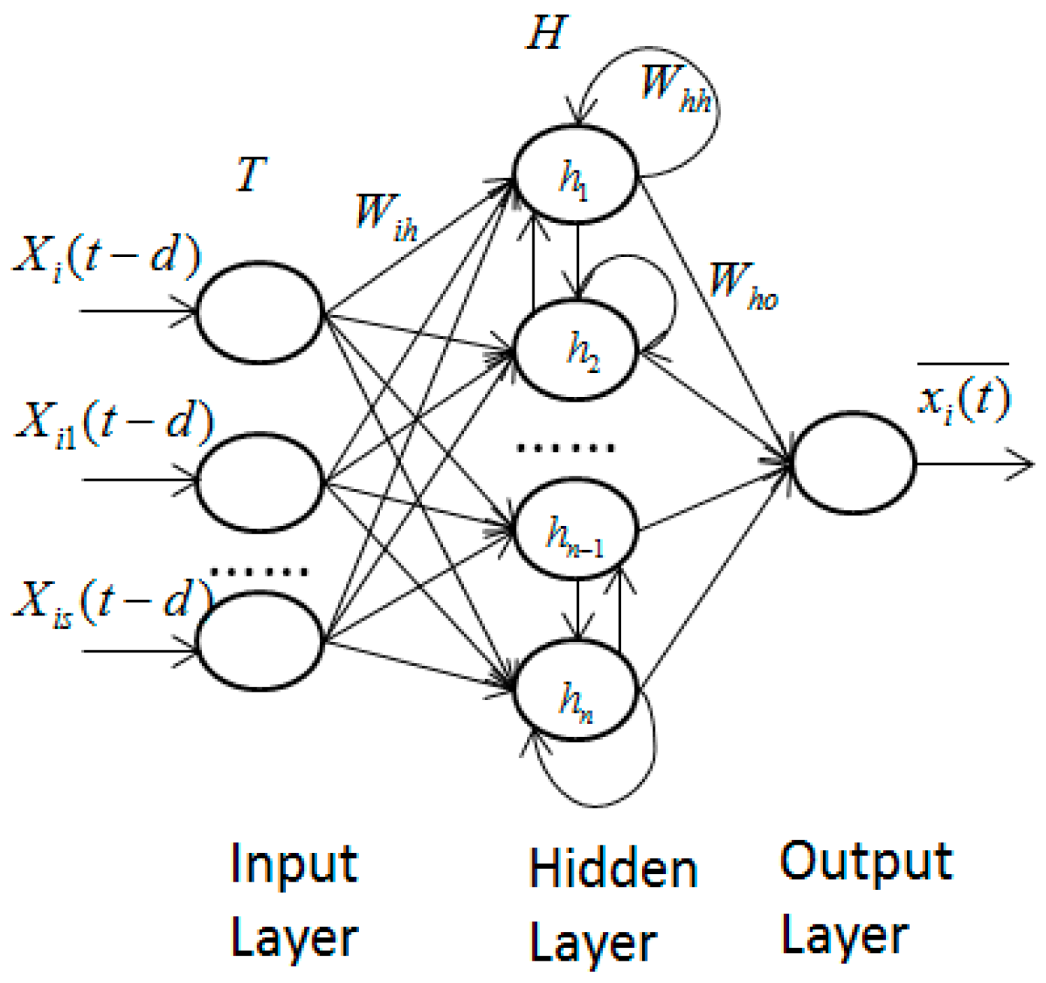
LSTM was proposed by Hochreiter and Schmidhuber in 1997 [22]. It is a new kind of RNN, which is faster and easier to converge to the optimal solution than other traditional neural networks when dealing with time sequence prediction problems. A water quality prediction model based on LSTM is established in Figure 1. The inputs are observations of $X_i$ and $U=\{X_{i1},X_{i2},\dots X_{is}\}$ at previous $t-d$ historical moments denoted as $T$. The output is the prediction value of $X_i$ at the tth moment denoted as $\overline{x_i(t)}$. The model consists of three layers: the input layer, the hidden layer, and the output layer. The weight between the input layer and the hidden layer is represented as $W_{ih}$. The neurons of the hidden layer are denoted as $H=(h_1,h_2,\dots ,h_j)$, where the jth neuron of the hidden layer is expressed as $h_j$. The weight within the hidden layer is denoted as $W_{hh}$. The weight between the hidden layer and output layer is represented as $W_{ho}$.

The calculation of the model is shown as follows:

$$h_n=H(W_{ih}T+W_{hh}{h}_{n-1}+b_h)$$

(10)

$$\overline{x_i(t)}=W_{ho}H+b_y$$

(11)

In the above formulas, the bias vector of the hidden layer is denoted as $b_h$ and the bias vector of the output layer is denoted as $b_y$.

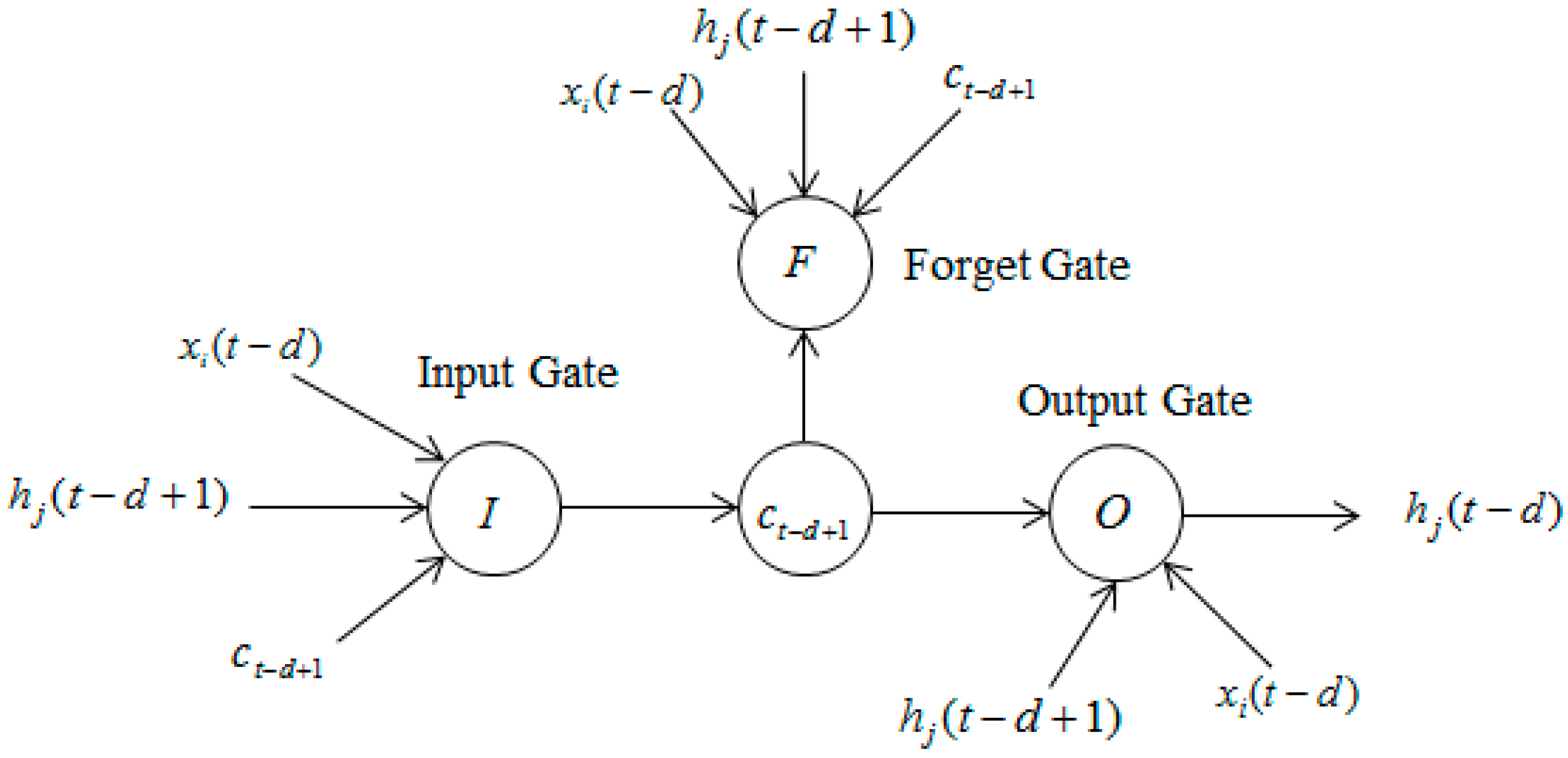
Each neuron of hidden layer in Figure 1 consists of three gates: the input gate, the output gate, and the forget gate. The structure of LSTM neuron is shown in Figure 2.

In Figure 2, the forget gate determines which part of the information should be forgotten according to the current input $x_i(t-d)$, the last moment state of the neuron $c_{t-d+1}$ and the last moment output of the jth neuron $h_j(t-d+1)$ in the hidden layer. The input gate determines which part of the information should be the input of the current moment state $c_{t-d}$ according to $x_i(t-d)$, $c_{t-d+1}$ and $h_j(t-d+1)$. The output gate determines the output of the current moment state according to the $c_{t-d}$, $h_j(t-d+1)$ and $x_i(t-d)$.

The calculation of the forget gate is shown as follows:

$$F=\sigma (W_{fi}{x}_i(t-d)+W_{fc}{c}_{t-d+1}+W_{fh}{h}_j(t-d+1)+b_f)$$

(12)

The calculation of the input gate is shown as follows:

$$I=\sigma (W_{Ii}{x}_i(t-d)+W_{Ic}{c}_{t-d+1}+W_{Ih}{h}_j(t-d+1)+b_I)$$

(13)

The calculation of the update state in the neuron is shown as follows:

$$c_t=F*c_{t-d+1}+I*g(W_{ci}{x}_i(t-d)+W_{ch}{h}_j(t-d+1)+W_{cc}{c}_{t-d+1}+b_c)$$

(14)

The calculation of the output gate is shown as follows:

$$O=\sigma (W_{oi}{x}_i(t-d)+W_{hh}{h}_j(t-d+1)+W_{oc}{c}_{t-d+1}+b_o)$$

(15)

The calculation of the hidden layer at the tth moment is shown as follows:

$$h_j(t-d)=o_t*P(c_{t-d+1})$$

(16)

In the above formulas, the sigmoid function is represented as $\sigma$. $g$ and $P$ are the extensions of stand sigmoid function with the value ranges of [−2, 2] and [−1, 1], respectively. $W_{fi}$, $W_{fc}$, and $W_{fh}$ are the weights between the forget gate and the input layer, the state unit, the hidden layer, respectively. $W_{Ii}$, $W_{Ic}$ and $W_{Ih}$ are the weights between the input gate and the input layer, the state unit, the hidden layer, respectively. $W_{ci}$, $W_{ch}$, and $W_{cc}$ are the weights between the state cell and the input layer, the hidden layer, the last moment state of the state cell, respectively. $W_{oi}$ and $W_{oc}$ are the weights between the output gate and the input layer, the state cell, respectively. The bias vectors of the forget gate, input gate, the state cell and the output layer are denoted as $b_f$, $b_I$, $b_c$, $b_o$, respectively. $*$ stands for the scalar product.

The selective memory function of LSTM is implemented by the gating mechanism that makes LSTM more suitable for dealing with time sequence prediction problems than other traditional neural networks. The water quality prediction model based on LSTM can take full advantage of the time sequence of the water quality information to improve the accuracy of prediction.

2.3. Water Quality Prediction Method Based on IGRA and LSTM

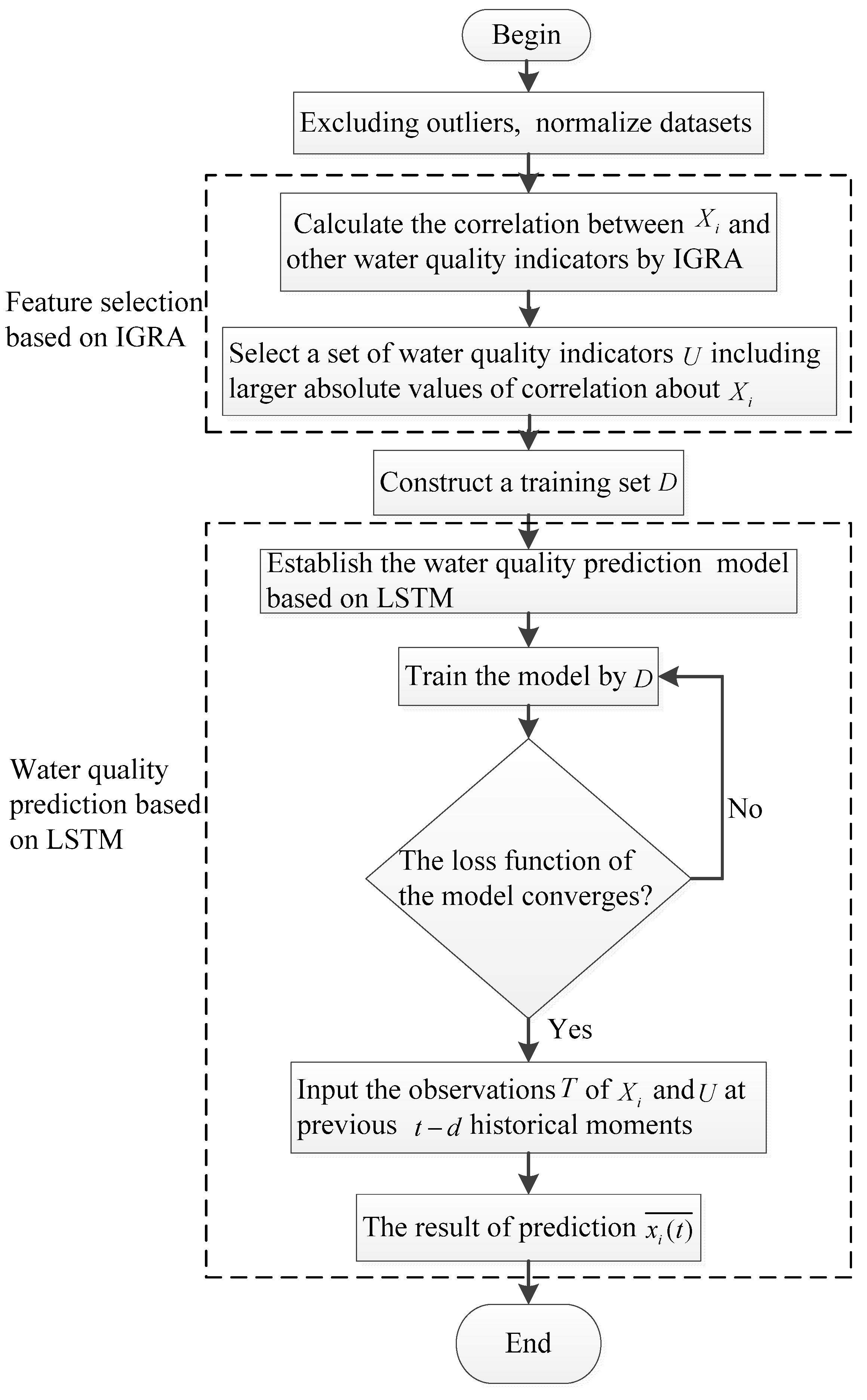
The procedure of water quality prediction method based on IGRA and LSTM is shown in Figure 3. In order to take full advantage of the multivariate correlation and time sequence of water quality information, the method in Section 2.1 is applied to select features from water quality information and the method in Section 2.2 is adopted to establish a water quality prediction model.

The specific steps for the prediction of the water quality indicator $X_i$ are shown as follows:

Step 1.

Exclude outliers based on Pauta criterion and normalize datasets.

Step 2.

Calculate the correlation between $X_i$ and other water quality indicators by IGRA.

Step 3.

Select a set of water quality indicators $U$ including larger absolute values of correlation about $X_i$. After that, construct a training set $D$.

Step 4.

Establish the water quality prediction model based on LSTM, train the model by $D$ until the loss function of the model converges.

Step 5.

Input the observations $T$ of $X_i$ and $U$ at previous $t-d$ historical moments to the model to acquire the prediction value $\overline{x_i(t)}$ of $X_i$ at the tth moment.

3. Results and Discussion

The experiment is implemented by advanced neural network toolkit Keras and TensorFlow. From our previous work [23], the optimal number of neuron nodes for each layer is 3, 8, and 1. The number of epochs is set to 50 and the proportion of training set and test set is set to 8:2. The proposed method is compared with other similar methods in two actual water quality datasets: Tai Lake and Victoria Bay.

3.1. Datasets

Tai Lake is the third largest fresh water lake in China, with a perimeter of about 400 kilometers. In recent decades, the industry and agriculture in the coastal areas of Tai Lake has developed rapidly, the water quality has been seriously polluted. In 2000, only 15% of the water bodies weren’t polluted, and the rest suffered varying degrees of pollution. The dataset of Tai Lake is composed of 648 monthly historical monitoring data collected from 8 monitoring stations between 2000 and 2006. It includes 10 water quality indicators: Total Nitrogen (TN), Total Phosphorus (TP), Ammonia Nitrogen (NH3-N), Suspended Solids (SS), Water Temperature (WT), Dissolved Oxygen (DO), Hydrogen Ion Concentration (pH), Transparency, Chloride (CL), and Precipitation.

Victoria Bay is the harbour between the Kowloon Peninsula and the Hong Kong Island in China. The area is about 41.88 km². It was formed more than 7000 years ago when the sea level was lower than it is now. In recent years, the content of DO in Vitoria Bay has been lower than the standard. The dataset of Victoria Bay is composed of 4283 historical monitoring data collected from 8 monitoring stations every two weeks between 1986 and 2016. It includes 9 water quality indicators: Escherichia coli (E. coli), 5th Biochemical Oxygen Demand (BOD5), NH3-N, Nitrite, Phosphate, pH, WT, Salinity, and DO.

It’s important to make water quality predictions for Tai Lake and Victoria Bay. The water quality indicator predicted in this experiment is DO.

3.2. Results of Feature Selection

This paper applies different relational analysis methods to calculate the correlation between DO and other indicators. The results of Tai Lake and Victoria Bay are shown in

Table 1. The relational analysis results of Tai Lake.

	WT	Precipitation	pH	NH3-N	Transparency	SS	TP	CL	TN
literature [20]	0.496	0.524	0.667	0.474	0.499	0.553	0.467	0.656	0.521
literature [21]	−0.166	0.018	0.112	−0.045	−0.043	−0.024	−0.021	0.023	−0.001
IGRA	0.566	0.347	0.183	−0.099	−0.088	−0.050	−0.045	0.044	−0.003

and

Table 2. The relational analysis results of Victoria Bay.

	Phosphate	WT	Nitrite	Salinity	NH3-N	BOD5	pH	E. coli
literature [20]	0.499	0.581	0.579	0.464	0. 590	0.565	0.460	0.554
literature [21]	−0.043	−0.166	0.257	0.018	−0.048	−0.017	0.011	−0.006
IGRA	−0.879	0.579	0.519	0.456	−0.085	−0.035	0.021	−0.013

.

It is obvious from Table 1 and Table 2 that compared with grey relational analysis used in literature [20], IGRA cannot only measure the positive correlation but also the negative correlations between DO and other water quality indicators. Compared with grey relational analysis algorithm in terms of similarity in literature [21], the results of IGRA in term of the similarity and proximity are more consistent with the results of qualitative analysis.

To further verify the effectiveness of IGRA, 4 indicators in the above tables, each of which has larger absolute correlation with DO, are selected as input features for the prediction model based on LSTM. The prediction errors of Tai Lake and Victoria are shown in

Table 3. Feature selection and prediction error of Tai Lake.

	Features	RMSE
literature [23]	DO	0.089
literature [20]	DO, pH, CL, SS	0.082
literature [21]	DO, WT, pH, NH3-N	0.079
IGRA	DO, WT, Precipitation, pH	0.074

and

Table 4. Feature selection and prediction error of Victoria Bay.

	Features	RMSE
literature [23]	DO	0.084
literature [20]	DO, NH3-N, Nitrite, BOD5	0.083
literature [21]	DO, Nitrite, WT, NH3-N	0.071
IGRA	DO, Phosphate, WT, Nitrite	0.065

.

From Table 3 and Table 4, compared with literature [23], which adopts only one feature DO for prediction, the results of the method with multiple features as inputs are better. Compared with the grey relational analysis algorithms in literature [20] and literature [21], the prediction error (root mean square error, RMSE) is smaller when the features are selected by IGRA. It suggests that IGRA can fully take advantage of the multivariate correlation of water quality information, which is effective for improving the accuracy of prediction.

3.3. Results of Water Quality Prediction

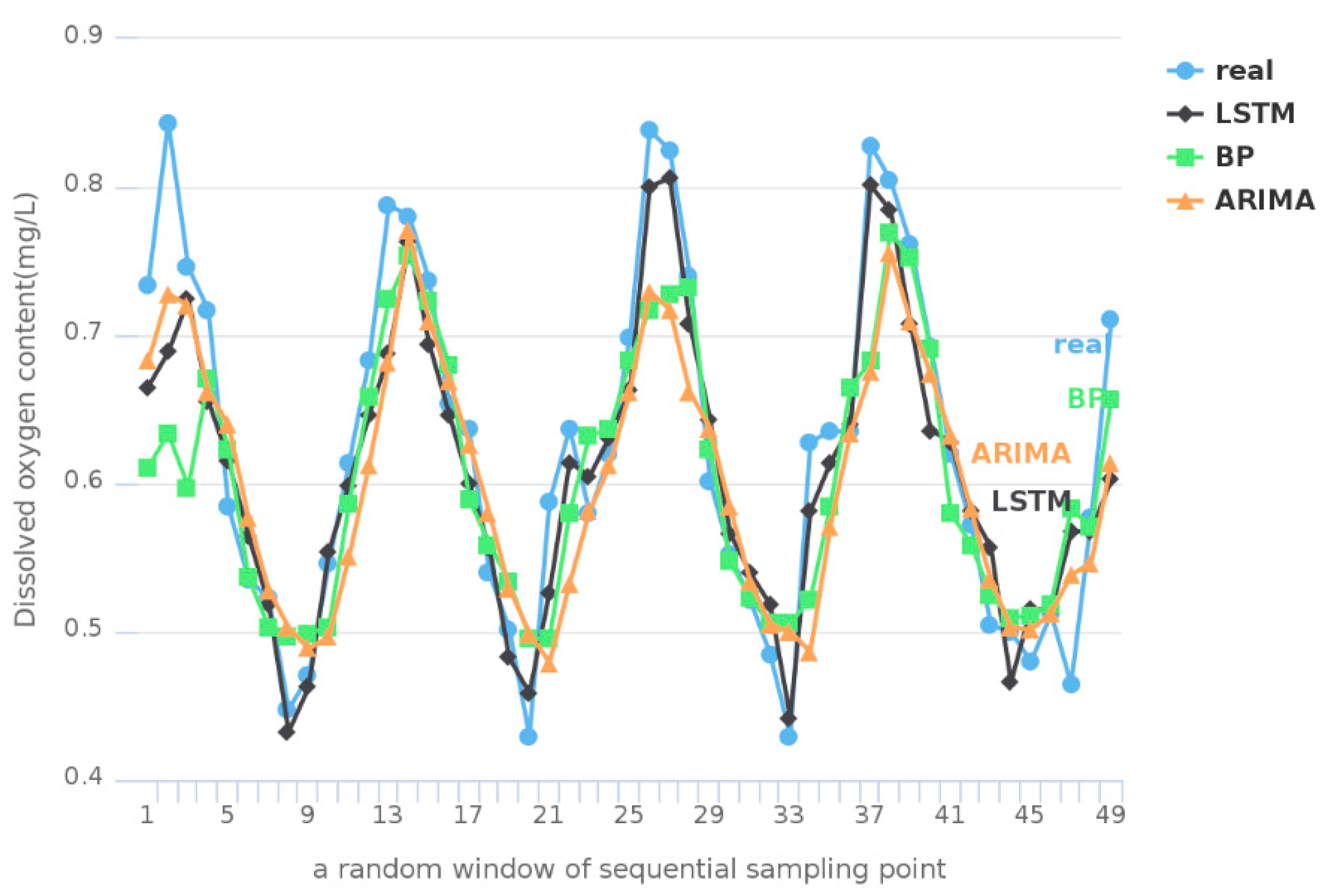
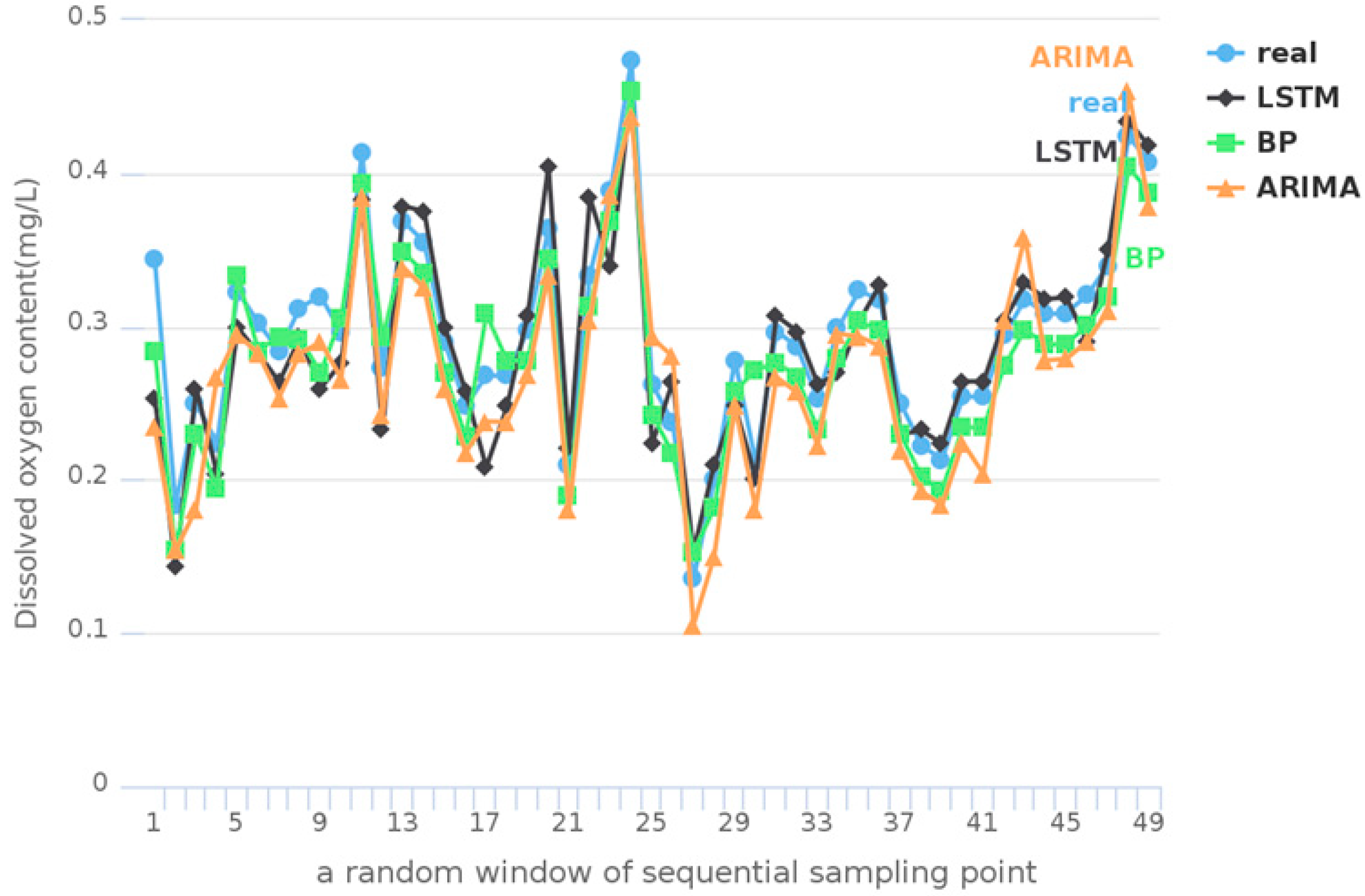
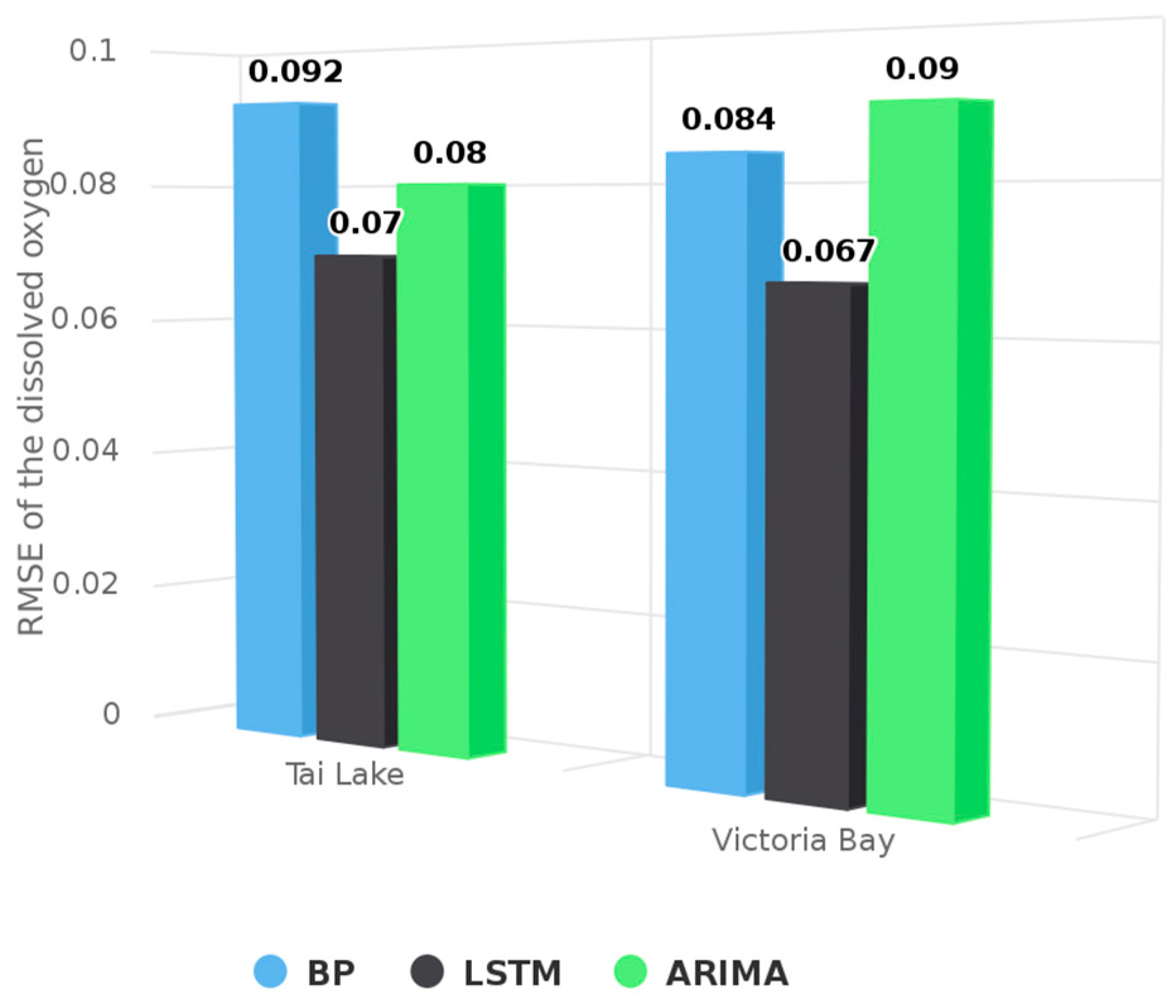
The result of feature selection for Tai Lake through IGRA is shown in the fourth row of Table 3. The result of feature selection for Victoria Bay is shown in the fourth row of Table 4. The comparison among DO prediction results of LSTM, Back Propagation (BP) neural network, and Auto Regressive Integrated Moving Average (ARIMA) model with the same inputs are shown in Figure 4 and Figure 5. RMSE of methods mentioned above is shown in Figure 6.

The prediction results in a random window of sequential sampling points from the test data set are shown in Figure 4 and Figure 5. According to these, the results of LSTM are closer to the real observations. It indicates that the prediction model based on LSTM is more accurate than other models based on BP or ARIMA. The RMSE for the entire test data set is shown in Figure 6. According to the Figure 6, the RMSE of LSTM is lower than that of BP and ARIMA in Tai Lake and Victoria Bay. It suggests that LSTM can fully take advantage of the time sequence of water quality information, which is effective for improving the accuracy of prediction.

4. Conclusions

Water quality prediction has great significance for water environment protection. Considering the multivariate correlation and time sequence of water quality information, a water quality prediction method based on IGRA and LSTM is proposed in this paper. First, IGRA is proposed to select features that are the indicators with a larger absolute correlation with the indicator to predict. In the second place, a prediction model based on LSTM is established, whose inputs are the indicators obtained by IGRA. The proposed method is compared with other similar methods in two actual water quality datasets: Tai Lake and Victoria Bay.

The experiment results demonstrate the following: (a) that IGRA can take full advantage of the multivariate correlation of water quality information and effectively select out the main impact indicators for the indicator to predict, and (b) that the prediction model based on LSTM can make the best use of the time sequence of water quality information and improve the accuracy of prediction. However, enough water quality indicators are required to use IGRA to make feature selection, and a large amount of historical monitoring data is required for training prediction models based on LSTM. In addition, the training time is somewhat long. Due to the complex structure of LSTM neurons, without the help of GPU, a training cycle which includes 100 iterations takes about 30 min. It is considered to improve the structure of the neurons for shorter training time in the future.

References

- Li, X.; Sha, J.; Wang, Z.L. Chlorophyll-A Prediction of lakes with different water quality patterns in China based on hybrid neural networks. Water 2017, 9, 524. [Google Scholar] [CrossRef]
- Grbić, R.; Kurtagić, D.; Slišković, D. Stream water temperature prediction based on Gaussian process regression. Expert Syst. Appl. 2013, 40, 7407–7414. [Google Scholar] [CrossRef]
- Candelieri, A. Clustering and support vector regression for water demand forecasting and anomaly detection. Water 2017, 9, 224. [Google Scholar] [CrossRef]
- Dai, Z.J.; Peng, X.C.; Huang, H. Application of grey model theory in prediction of river water pollution. Environ. Assess. 2002, 1, 28–29. [Google Scholar]
- Bougadis, J.; Adamowski, K.; Diduch, R. Short-term municipal water demand forecasting. Hydrol. Process. 2005, 19, 137–148. [Google Scholar] [CrossRef]
- Jain, A.; Ormsbee, L.E. Short-term water demand forecast modeling techniques-Conventional methods versus AI. J. Am. Water Works Assoc. 2002, 94, 64–72. [Google Scholar] [CrossRef]
- Adamowski, J.F. Peak daily water demand forecast modeling using artificial neural networks. J. Water Resour. Plan. Manag. 2008, 134, 119–128. [Google Scholar] [CrossRef]
- Bakker, M.; Duist, H.V.; Schagen, K.V.; Vreeburg, J.; Rietveld, L. Improving the performance of water demand forecasting models by using weather input. Procedia Eng. 2014, 70, 93–102. [Google Scholar] [CrossRef]
- Chen, Y.H.; Rangarajan, G.; Feng, J.F.; Ding, M.Z. Analyzing multiple nonlinear time series with extended granger causality. Phys. Lett. A 2004, 324, 26–35. [Google Scholar] [CrossRef]
- Patton, A. Copula methods for forecasting multiple times series. In Handbook of Economic Forecasting; Elsevier: Amsterdam, The Netherlands, 2013; pp. 899–960. [Google Scholar]
- Deng, J.L. Introduction to grey system theory. J. Grey Syst. 1989, 1, 1–24. [Google Scholar]
- Maier, H.R.; Dandy, G.C. The use of artificial neural networks for the prediction of water quality parameters. Water Resour. Res. 1996, 32, 1013–1022. [Google Scholar] [CrossRef]
- Bazartseren, B.; Hildebrandt, G.; Holz, K.P. Short term water level prediction using neural networks and neuro-fuzzy approach. Neurocomputing 1996, 55, 439–450. [Google Scholar] [CrossRef]
- Xu, L.; Liu, S. Study of short-term water quality prediction model based on wavelet neural network. Math. Comput. Model. 2014, 58, 807–813. [Google Scholar] [CrossRef]
- Jain, A.; Varshney, A.K.; Joshi, U.C. Short-term water demand forecast modelling at IIT Kanpur using artificial neural networks. Water Resour. Manag. 2001, 15, 299–321. [Google Scholar] [CrossRef]
- Ghiassi, M.; Zimbra, D.K.; Saidane, H. Urban water demand forecasting with a dynamic artificial neural network model. J. Water Resour. Plan. Manag. 2008, 134, 138–146. [Google Scholar] [CrossRef]
- Williams, R.J.; Peng, J. An efficient gradient-based algorithm for on-line training of recurrent network trajectories. Neural Comput. 1990, 2, 490–501. [Google Scholar] [CrossRef]
- Jiang, Q.; Tang, C.; Chen, C.; Wang, X.; Huang, Q. Stock price forecast based on LSTM neural network. In Proceedings of the Twelfth International Conference on Management Science and Engineering Management, Melbourne, Australia, 1–4 August 2018; pp. 393–408. [Google Scholar]
- Ma, X.L.; Ma, X.; Tao, Z.; Wang, Y.; Yu, H.; Wang, Y. Long short-term memory neural network for traffic speed prediction using remote microwave sensor data. Transp. Res. 2015, 54, 187–197. [Google Scholar] [CrossRef]
- Liu, S.F.; Xie, N.M.; Jeffery, F. A new grey relational analysis model based on similarity and proximity perspective. Syst. Eng. 2010, 30, 881–887. [Google Scholar]
- Han, M.; Zhang, R.Q.; Xu, M.L. A variable selection algorithm based on improved grey relational analysis. Control Decis. 2017, 32, 1647–1652. [Google Scholar]
- Hochreiter, S.; Schmidhuber, J. Long short-term memory. Neural Comput. 1997, 9, 1735–1780. [Google Scholar] [CrossRef] [PubMed]
- Wang, Y.Y.; Zhou, J.; Chen, K.J.; Wang, Y.Y.; Liu, L.F. Water quality prediction method based on LSTM neural network. In Proceedings of the 12th International Conference on Intelligent Systems and Knowledge Engineering, Nanjing, China, 24–26 November 2017; pp. 1–5. [Google Scholar]
Figure 1.
Water quality prediction model based on LSTM.
Figure 2.
Structure of LSTM neuron.
Figure 3.
Flow chart of water quality prediction method based on IGRA and LSTM.
Figure 4.
Prediction results of Tai Lake.
Figure 5.
Prediction results of Victoria Bay.
Figure 6.
RMSE of BP, LSTM and ARIMA.