Improved Inverse Modeling by Separating Model Structural and Observational Errors


1
State Key Laboratory of Hydrology Water Resources and Hydraulic Engineering, Hohai University, Nanjing 210098, China
2
College of Hydrology and Water Resources, Hohai University, Nanjing 210098, China
*
Author to whom correspondence should be addressed.
Water 2018, 10(9), 1151; https://doi.org/10.3390/w10091151
Submission received: 10 July 2018
/
Revised: 21 August 2018
/
Accepted: 25 August 2018
/
Published: 28 August 2018
(This article belongs to the Section Hydrology)
Abstract
:A practical formal likelihood function (L) is developed to separate model structure errors and observation errors by the separation of correlated and uncorrelated model residuals. L overcomes the time-consuming problem of likelihood functions proposed by previous studies, and combines the Mean Square Error (MSE) and first-order Auto-Regression (AR(1)) models. For comparison of the effect of different error models, MSE, AR(1), and L are used as efficiency criteria to calibrate the three-dimensional variably saturated ground-water flow model (MF2K-VSF) based on the soil tank seepages of rainfall–runoff experiments. Results of L are nearly the same as those of AR(1) due to negligible observational errors. Although all calibrated models well mimic the seepage discharges, MF2K-VSF with MSE cannot capture the groundwater level and soil suction processes because of the considerable autocorrelation of model residuals owing to model inadequacies (e.g., neglect of the soil moisture hysteresis), which obviously violates the statistical assumption of MSE. By contrast, L accounts for the model structural errors and thus enhances the reliability of hydrological simulations.
1. Introduction
Numerical groundwater models (such as three-dimensional finite-difference ground-water model (MODFLOW), three-dimensional variably saturated ground-water flow model (MF2K-VSF), and Hydrus) are widely used for groundwater resource assessment [1,2]. Although parameters of a numerical groundwater model have definite physical meaning and can be estimated in the field or laboratory at a specific location, scale effects due to the aquifer heterogeneity often hinder their accurate estimations [3,4,5,6]. Therefore, for improvement of model performance, a so-called inverse modeling is popularly proposed to calibrate groundwater models, which iteratively adjusts the model parameters so that model outcomes approximate, as closely and consistently as possible, the historical record data [3,6,7].
Unlike the manual calibration method, inverse modeling impossibly uses the visual inspection of similarities and differences between model predictions and observed data. Therefore, hydrologists have proposed many statistical measures as model efficiency criteria instead of subjective visual judgment to ascertain the goodness of fit of hydrologic models [8,9,10,11,12]. Among these goodness-of-fit indicators, the mean squared error (MSE) (i.e., standard least squares) and its normalization (i.e., Nash–Sutcliffe efficiency (NSE) defined by Nash and Sutcliffe [13] are most widely used [7,9,12,14,15,16].
With the development of Bayesian theory (e.g., maximum likelihood Bayesian model averaging approach [17,18,19]), the likelihood function is widely concerned because of the powerful theoretical support [6,20]. The likelihood function is defined as the joint probability of model residuals. The maximum likelihood value is in agreement with the best model parameters, which is the so-called maximum likelihood estimation. Moreover, some statistical measures can be reevaluated from the likelihood function viewpoint [16]. For example, numerous authors [14,21,22] pointed out that MSE implies statistical assumptions that model errors should be independent and identically distributed (I.I.D.) according to a Gaussian distribution with zero mean and a constant variance. However, Beven et al. [23] believed that model residuals rarely fulfill the I.I.D. assumption in practice because they do not only have random components but also include epistemic errors (e.g., model structure errors) that result in the bias, correlation, and heteroscedasticity of model residuals. Therefore, it is necessary to explicitly account for the epistemic errors (i.e., nonrandom components) before calculation of the probability densities of model residuals [24]. The first-order autoregressive (AR(1)) scheme and the Box–Cox transformation method are popularly used to remove the correlation and heteroscedasticity of model residuals, respectively [24,25,26,27].
Reichert and Mieleitner [28] pointed out that the model residuals come from several parts: the model input error, the model parameter error, the model structural error, and the observed output error. Because model parameter and input errors affect the model residual through model structure, model structural errors in this study include the model parameter and input errors. However, traditional methods (e.g., AR(1)) lump all errors of model structure and observation into a single additive residual term, but neglect the distinctions of error sources. In fact, the error characteristics of different error sources are different. For example, the model structure errors have a high degree of temporal correlation [29], while the observational errors are usually independent [30]. Therefore, it is unreasonable to simultaneously account for the correlation of model structural and observational errors by the AR(1) method. Overall, a formal likelihood function could be able to distinguish errors from model structure and observation and remove their nonrandom components [23], because I.I.D. model residuals are convenient for estimation of their joint probability. For this purpose, Reichert and Schuwirth [30] proposed a formal likelihood function based on the assumption that both the model structural and observational errors follow the multivariate Gaussian distribution.
In the multivariate Gaussian distribution, the covariance matrix reflects the correlation between any two variates, and the inverse covariance matrix should be calculated before estimation of the joint probability of variates. However, it is time-consuming to compute the inverse matrix, e.g., the widely used lower–upper (LU) decomposition algorithm costs about 2n3/3 floating point operations, where n is the number of variates (i.e., the dimension of the covariance matrix) [31]. Therefore, the direct estimation of likelihood function values proposed by Reichert and Schuwirth [30] can pose serious numerical problems when calculating the highly dimensional inverse covariance matrix [30,32]. In other words, the likelihood function is inapplicable for the long hydrologic series. Nevertheless, a success of inverse modeling requires sufficient observation data [33]. As a consequence, the likelihood function introduced by Reichert and Schuwirth [30] seems unworkable in practice at the moment.
In order to overcome the numerical problems, this study attempts to simplify the likelihood function introduced by Reichert and Schuwirth [30], and find an analytical solution of the inverse covariance matrix to save computational time. Herein, we firstly develop a (practical) formal likelihood function to separate model structural and observational errors based on the assumptions that (1) the correlated residuals only originate from the model structural errors [29], (2) the AR(1) scheme can remove the correlation of model residuals [24,25,26,27], and (3) the observational errors follow a Gaussian distribution with an identical variance [30]. Then the new likelihood function and analytical solution are tested by synthetically generated data. Next, we apply the (practical) formal likelihood function as an efficiency criterion to calibrate the numerical groundwater model (MF2K-VSF) based on the soil tank seepage data of two rainfall–runoff experiments. At last, for assessment of the effects of efficiency criteria on the inverse modeling, the model calibration results of seepages together with soil suctions and groundwater levels for the formal likelihood function are compared with those for the traditional efficiency criteria (i.e., MSE and AR(1) methods).
2. Methods
2.1. Equivalent Relationship between AR(1) and Multivariate Gaussian Distribution
The errors/residuals (e) between the observed and the simulated outcomes are treated as random variables:
where and are observed and simulated outcomes at time step i, respectively.
In the dynamics-based groundwater model, the model outputs depend heavily on their previous state, which results in the “memory” of model predictions. Therefore, model residuals usually exhibit considerable autocorrelation as a result of the groundwater model inadequacies [24,29]. The first-order autoregressive (AR(1)) scheme is widely used to remove the autocorrelation of model residuals:
where is the model residual after AR(1), R is the autocorrelation coefficient of the model residuals, and and are the original model residuals at the time steps i − 1 and i, respectively.
If model residuals after AR(1) follow the Gaussian distribution, the logarithmic (log-) likelihood function can be expressed as
where n is the length of the model residual series, is the standard deviation of model residuals after AR(1), and is the standard deviation of and usually .
Defining Λ as
and E as the vector of model residuals
then Equation (3) can be simplified as
where is the determinant of matrix , and is the transposition of the vector E.
Because the inverse matrix of is [34]
Equation (4) can be expressed as
where is the covariance matrix of model residuals.
Equation (5) reveals that the model residuals follow the multivariate Gaussian distribution with the covariance matrix as the model residuals after AR(1) follow the Gaussian distribution. In other words, if the model residuals follow the multivariate Gaussian distribution with , AR(1) can remove the autocorrelation of model residuals.
2.2. A Practical Formal Likelihood Function to Separate Model Structural and Observational Errors
Based on the assumptions that both the model structural and observational errors follow the multivariate Gaussian distribution, Reichert and Schuwirth [30] derived a formal likelihood function to distinguish errors from model structure and observation:
where is the covariance matrix of model structure errors, is the standard deviation of observational errors, is the identity matrix, and is the covariance matrix of observational errors.
The mean of the observational error conditional distribution given model residuals (E) is
and the model structural error mean is
The calculation of the inverse covariance matrix is the main barrier of this likelihood function application [30,32]. Reichert and Schuwirth [30] point out that the theoretical development of a formal likelihood function is independent of the specific form of . In Section 2.1, has been proved to be a covariance matrix of AR(1) that is able to represent the first-order autocorrelation of model structure errors [24,26]. Therefore, in this study, we use the specific covariance matrix ( in Equation (5)) to replace in order to save computational time:
Equation (9) has the analytical solution (see Appendix A for technical details). After substituting Equation (9) into Equation (6) and defining , the log-likelihood function (Equation (6)) is transformed to
The formal likelihood function (L; Equation (10)) is flexible. When b = 0, L becomes
Equation (11) is equivalent to MSE [22], where model residuals only include the observational errors. Therefore, MSE actually neglects any model inadequacies and attributes deviations between model predictions and observed data to measurement errors.
When b approaches infinity, L (Equation (10)) becomes
Equation (12) is the same as Equation (4) of AR(1), which means that the model residuals only include the model structural errors. In other words, the assumption of AR(1) is that the model residuals do not include the observational errors.
When
the practical likelihood function Equation (10) reaches the maximum value:
The practical formal likelihood function (Equation (14)) has two statistical parameters: R which is the autocorrelation coefficient of model structural errors, and b which is the ratio between the variance of the random components of model structural errors and the variance of the observation errors.
2.3. Test of the Practical Formal Likelihood Function
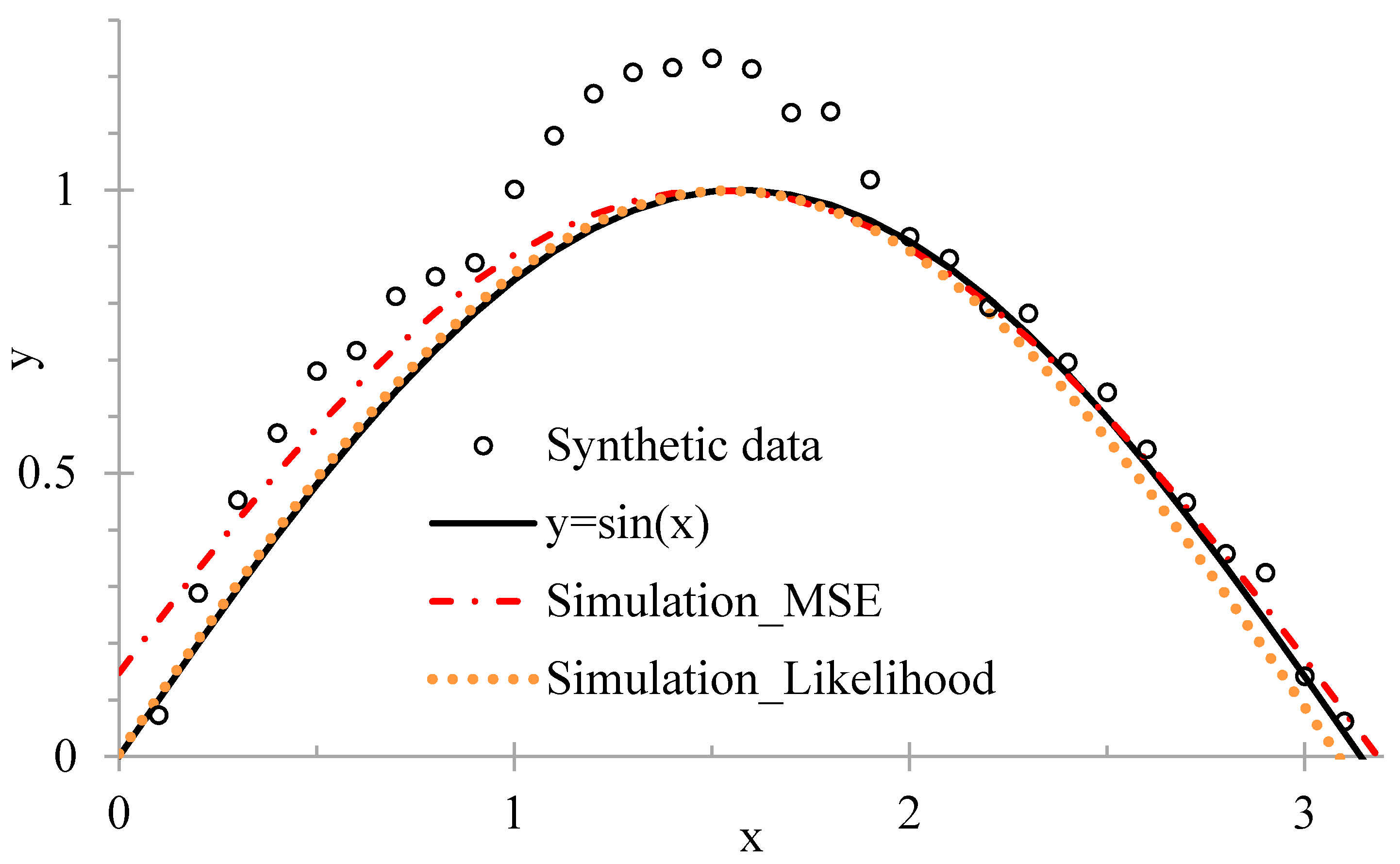
We assume that y = sin(c × x + d) is a model, of which c and d are the parameters. When c = 1, d = 0, R = 0.9, b = 4, and σe = 0.02, the synthetic observation values of the model can be generated using the following equation:
where emod and eobs are the errors of model structure and observation, respectively. emod follows the random distribution of Equation (5), and eobs follows the Gaussian random distribution (Equation (11)). An example of synthetic observation data is shown in Figure 1.
For comparison of the computational efficiency of the analytical solution and inverse matrix approach, different lengths of observed data series are generated by Equation (15), and the runtimes of the two methods for different numbers of observed data are shown in Table 1. Table 1 indicates that the elapsed time increases with the length of the data series. However, the analytical solution is much faster than the inverse matrix approach, and the inverse matrix approach even fails to proceed because of lack of memory when there are too many datapoints, i.e., high-dimension covariance matrix. Therefore, the analytical solution proposed by this study is faster than the inverse matrix approach.
In order to compare the effects of different model calibration criteria, 33 synthetic observation datapoints were generated (Figure 1), of which small samples can emphasize the difference in model calibration results. The model calibration results of the MSE, AR(1), and L methods are shown in Table 2, and the simulation results are presented in Figure 1. Table 2 indicates that the optimized parameter values for L are much closer to the true values of the model (i.e., y = sin(x)) than are those for MSE. There is an obvious tradeoff between the model efficiency criteria of MSE and L. Therefore, L and MSE are two different criteria. Because MSE only considers the observed errors, the model structure errors with strong autocorrelation easily affect the calibration results. By contrast, L proposed by this study can filter the effect of model structural errors to obtain more reliable model parameters. Because the value of b (i.e., equal to 4) is large, which means that model residuals primarily come from model structure errors and the observation errors are negligible, the optimized results of the AR(1) method are similar to those of the L approach.
In summary, the analytical solution is much faster than the matrix inversion method, and the inverse model with L identifies model parameter values better than that with MSE.
3. Case Study
3.1. Material
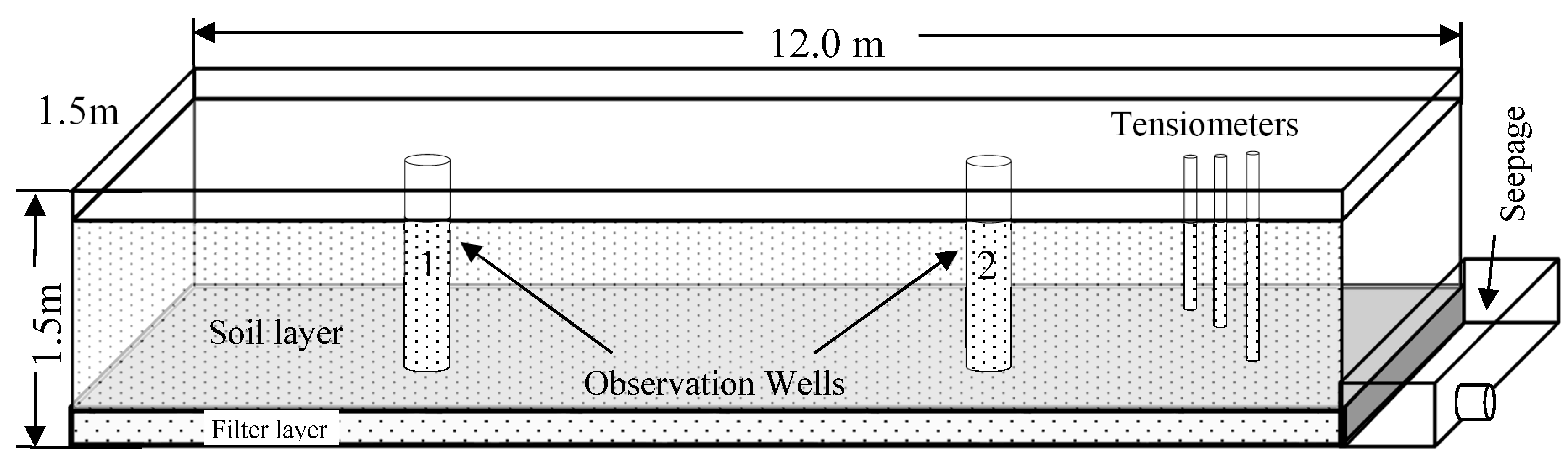
The test data were collected from rainfall–runoff experiments within a soil tank (Figure 2) in the State Key Laboratory of Hydrology, Water Resources and Hydraulic Engineering at Hohai University, China. The size of the soil tank is 12 m in length, 1.5 m in width, and 1.5 m in height. In the soil tank, we first laid a 5.0 cm thick filter layer with coarse gravel, and then filled in a 1.3 m thick soil layer with dried and sieved sandy loam in 2004. The total thickness was equal to 1.35 m. The proportions of soil particle size were 7.1% clay, 16.4% silt, and 76.5% sand. After dozens of rainfall experiments, the structure of the soil approached a steady state with saturated water content of 0.40 and dry bulk density of 1.40 g/cm3. As shown in Figure 2, a small tank was connected to the soil tank to gather the seepage flow from the filter layer, and its seepage height was set to 6.2 cm to submerge the 5.0 cm thick filter layer.
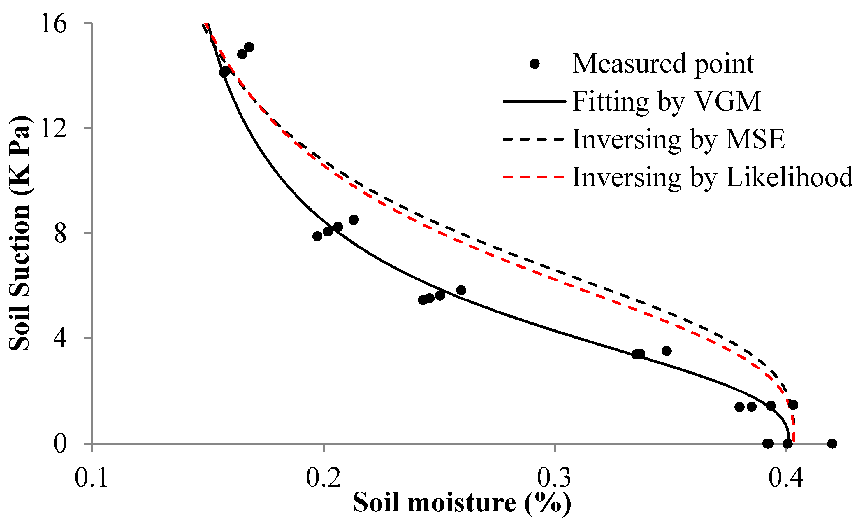
We sampled some soil cores on the surface of the soil tank for measurement of the soil hydraulic properties in the laboratory. The falling head method was used to estimate the vertical soil hydraulic conductivity of soil cores [5,35]. The result was equal to 6.884 ± 2.268 × 10⁻⁶ m/s. A refrigerated centrifuge (CR21GIII, Hitachi Koki Co., Ltd., Tokyo, Japan) was used to measure the soil water retention curve. The results are presented in Table 3 and Figure 3. Note that the positive value of soil suction means that soil is unsaturated, rather than saturated, which is opposite to the value of the water pressure head.
Three rainfall–runoff experiments were executed. The first experiment with a rainfall intensity of 2.1 mm/min lasted 1.8 h, the second of 1.7 mm/min lasted 4.2 h, and the third of 1.4 mm/min lasted 1.4 h. Most of the rainfall became surface runoff. However, to increase infiltration, the outlet of the surface drainage ditch was blocked in the third experiment. The seepage from the filter layer was observed using a highly precise tipping bucket gauge. In the third experiment, however, in order to avoid limitation of the measurement range (from 0 to 1.3 × 10⁻³ m3/min) of the tipping bucket gauge, we first manually measured the peak of seepage over the limitation and then automatically measured the seepage using the tipping bucket gauge. Of course, the accuracy of the manual observation is worse than that of the tipping bucket gauge. The soil suction was measured by tensiometers with porous ceramic cups at the depths of 80, 100, and 130 cm, and the groundwater level was measured by wells with automatic observation sensors (HOBO® U20 Water Level Logger). The position of tensiometers and wells is shown in Figure 2. Note that the locations of tensiometers close to the outlet of the sandbox is for avoiding the effect of groundwater. The precisions of the rainfall gauge, tipping bucket gauge, water level logger, and tensiometer were ±1.0%, ±1.0%, ±0.1%, and ±0.5% full scale, respectively. The automatic measurement frequencies of seepage, soil suction, and groundwater level were all 1 min, and the manual measurement frequency of seepage was about 10 min.
3.2. Numerical Groundwater Model
MF2K-VSF is a numerical groundwater model developed by United States Geological Survey (USGS), which can simulate three-dimensional variably saturated flow in porous media by expanding the saturated groundwater flow equation (used by MODFLOW) to include unsaturated flow using Richards’ Equation [1]. The governing equation for two-dimensional variably saturated flow is
where ψ is the pore water pressure head, h is the total hydraulic head, θ(ψ) is the soil water content as a function of the pore water pressure head, and Kx(ψ) and Kz(ψ) are the horizontal and vertical hydraulic conductivities, respectively, as functions of the pore water pressure head.
The van Genuchten–Mualem model (VGM) is widely used to estimate the soil water content and unsaturated hydraulic conductivity based on the pore water pressure head. For improving the flexibility of VGM functions, a dual set of parameters is used [1]:
where α1, n1, and m1 are the curve shape parameters of VGM for the unsaturated hydraulic conductivity; Ks is the saturated hydraulic conductivity; α2, n2, and m2 are the curve shape parameters of VGM for the soil water content; mi = 1 − 1/ni, i = 1, 2; θs is the saturated soil water content; and θr is the residual soil water content.
In Equation (17), θs and θr are estimated by fitting the soil water retention curve using the VGM model (Figure 3), and are identified as 0.40 and 0.10, respectively. Figure 2 shows that the soil tank can be divided into two layers: soil/upper layer and filter/lower layer. For the filter layer, because it is always saturated and shallow, only the hydraulic conductivity needs to be estimated (Kf in Table 3). For the soil layer, however, six parameters (α1, n1, α2, n2, and horizontal and vertical Ks) need to be estimated. The detailed descriptions of parameters for model calibration are given in Table 3.
In the numerical model, we perform two-dimensional (2D) simulation to save computational time, and the 2D model is sufficient and will provide accurate results because the ratio between the length and the width of the soil tank is large and the main flow is in the longitudinal direction. The grid size was set to (Horizontal) 10 cm × (Vertical) 1 cm, the time step size was 1 min, and the simulation periods of the three experiments were about 3, 5, and 6 days, respectively. The boundary conditions (BC) were the default BC of MF2K-VSF, i.e., no-flow BC. The drain package was used to simulate the seepages from the soil tank, and an improved lake package was used to simulate not only the rainfall infiltration but also the soil tank surface ponding recession. The improved lake package sets the lake cells as constant-head cells with the head of lake water level in the initial time-step, which will be updated in the next time-step according to the estimated infiltration rate.
The soil tank seepages of the first and the second rainfall–runoff experiments were selected to calibrate seven parameters of MF2K-VSF (Table 3). Then, the measured soil suctions and groundwater levels and the observed data of the third rainfall–runoff experiment were used for validation of the calibrated MF2K-VSF model. The peak seepage flows of the second rainfall–runoff experiment (Figure 4(a2nd)) were unfortunately lost because the seepage exceeded the measurement range of the tipping bucket gauge. However, the missing data affected the model calibration results only slightly because two rainfall–runoff experimental datasets were used to calibrate the numerical model and the peak seepage flows of the first rainfall–runoff experiment were captured which could overcome the mistake of data loss. Due to the long time interval (about 5 months) between the two rainfall–runoff experiments, the soil water was always in a relatively stable state at the beginning of each experiment. In this study, initial heads of the soil layer adopt the tensiometer measurement data.
The Differential Evolution Adaptive Metropolis (DREAM) Markov Chain Monte Carlo (MCMC) scheme was employed as the optimization tool in inverse modeling. This scheme is ideally suited for high-dimensional and multimodal optimization problems because it follows up on the Shuffled Complex Evolution Metropolis (SCEM-UA) global optimization algorithm, runs multiple different chains simultaneously for global exploration, and maintains a detailed balance condition [36]. In this study, the likelihood functions of MSE, AR(1), and L (i.e., Equations (10)–(12), respectively) were separately used as the model calibration criterion in DREAM. For each criterion, we selected 8 parallel chains and a total of 40,000 model evaluations for the DREAM algorithm parameterization on the R platform, and ran them on the “Soroban” High-Performance Computing System at Freie Universität Berlin. The running times of DREAM for MSE, AR(1), and L are about 14, 14, and 15 days, respectively. The operating speeds of the MSE and AR(1) methods are faster than that of the L approach.
4. Results
For comparison of the traditional least-squares estimation [7,15] and the maximum likelihood estimation, MSE (i.e., the standard least squares), AR(1), and L methods were selected as the efficiency criteria of inverse modeling to estimate the parameters of the numerical groundwater model (MF2K-VSF). The optimal values of model parameters are listed in Table 3. In this table, the values of the autocorrelation coefficient (R) are close to 1.0, which means that there is a considerable correlation of model residuals. The large value of the ratio (b = 3.0) demonstrates that the model structural errors are three times larger than the observed errors. As a consequence, the calibration results of the AR(1) method are nearly the same as those of the L approach because the observed errors can be neglected.
Optimal values of model parameters between MSE and L are different, particularly the horizontal hydraulic conductivity of soil and filter layers. Optimal model parameter values are different from the measurement results (Table 3 and Figure 3) possibly because the calibrated parameters are the “effective parameters” and represent the integrated behavior at the model element scale rather than at the field measurement point [3,4].
For the soil layer, the horizontal and vertical hydraulic conductivity from MSE is larger than that from L while for the filter layer, the hydraulic conductivity from the two methods presents the opposite relationship. This may result from the correlation relationship between the two layer parameters in the numerical model because the soil tank seepage would be compensated by the increased flow from the filter layer as the infiltration recharges decrease from the soil layer.
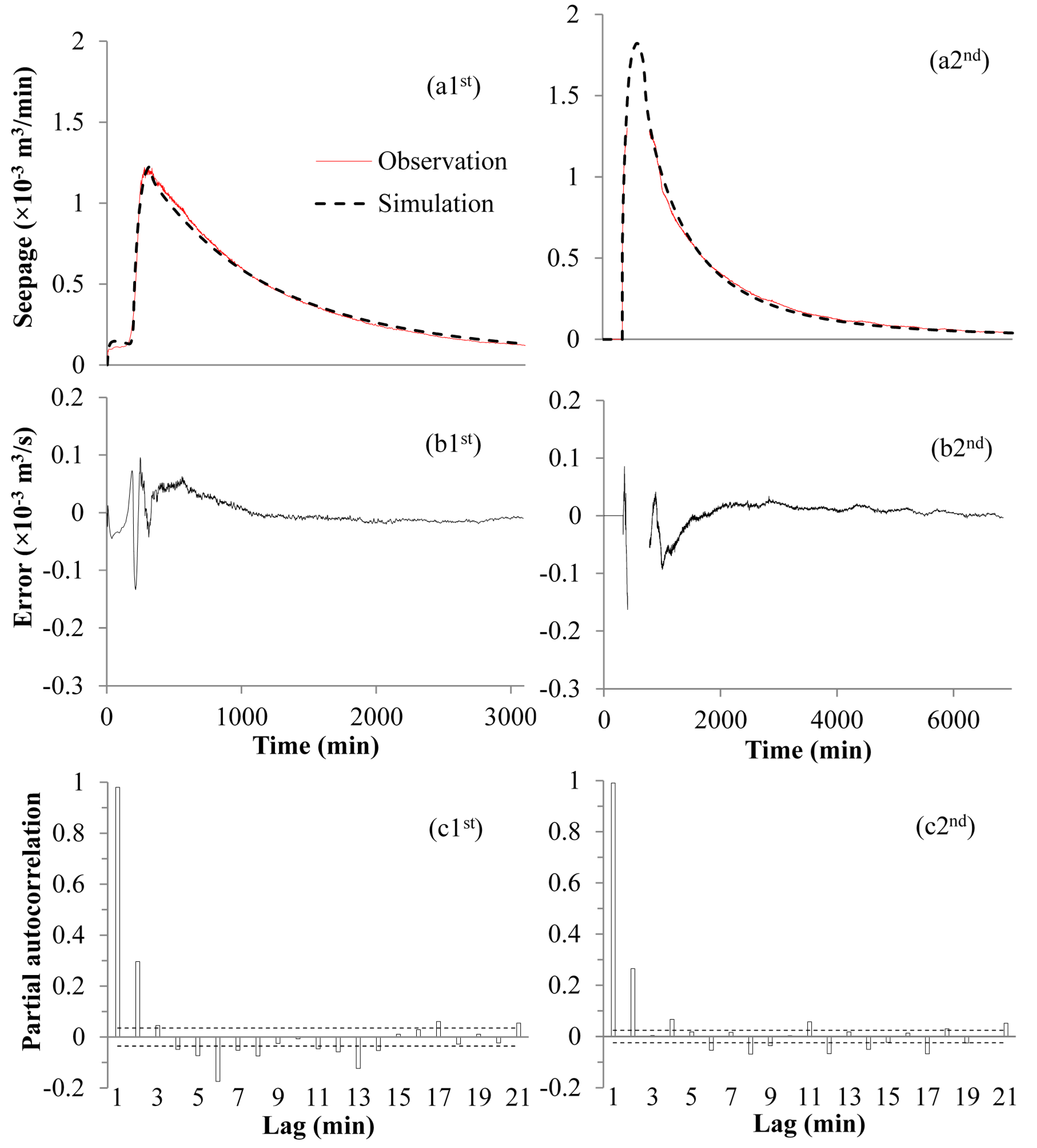
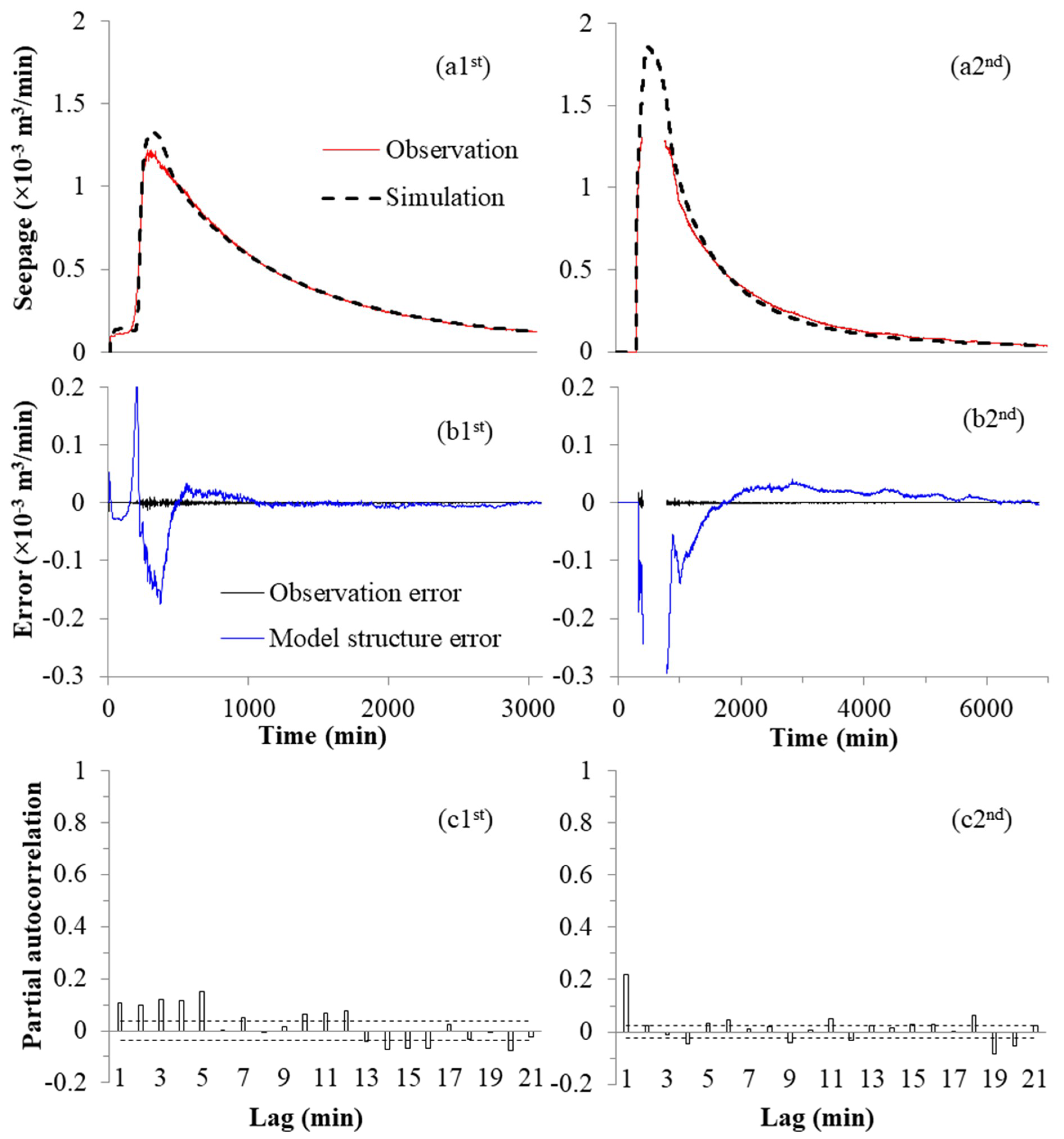
Error analysis for the simulated seepages of MF2K-VSF with MSE is shown in Figure 4. In this figure, a1st and a2nd show the seepage processes of the first two rainfall-runoff experiments; b1st and b2nd are their corresponding residuals; and c1st and c2nd diagnose the autocorrelation of model residuals by the partial autocorrelation plot. Figure 4(a1st,a2nd) show that MF2K-VSF with MSE mimics the seepage processes well, but its model residuals are significantly correlated at a lag of one minute (Figure 4(c1st,c2nd)), which violates the assumption of MSE that the model residuals should be independent [14,21,22]. Figure 4(b1st,b2nd) shows that most large model residuals gather around the peak seepage flow. A possible reason for this is that MF2K-VSF cannot capture the wetting and drying processes of soil moisture at the same, because MF2K-VSF neglects the hysteresis effect of soil moisture movement [1].
Error analysis for the simulated seepages of MF2K-VSF with L is shown in Figure 5. In this figure, b1st and b2nd decompose the model residuals into the model structural and observational errors according to Equations (7) and (8); and c1st and c2nd inspect autocorrelation of model structural errors after AR(1) by the partial autocorrelation plot. Figure 5(b1st,b2nd) indicate that the model structural errors are much greater than the observational errors, which is in agreement with the large value of b in Table 3. The negligible observation errors are due to the high-precision gauge of the laboratory measurement. The primary errors from the model structure indicate that the L method may have some advantages.
Compared with Figure 4(c1st,c2nd) and 5(c1st,c2nd) show that L obviously reduces the correlation of model residuals. Note that it is difficult or impossible to completely remove the errors’ correlation because of the complex error sources of model residuals, e.g., model input (such as rainfall and initial head) errors. Nevertheless, the larger range of model residuals in Figure 5b than in Figure 4b shows that the performance of model-simulated seepages for the MSE method is better than that for the L approach. Possibly, the MSE method over-calibrates the MF2K-VSF model [16,20].
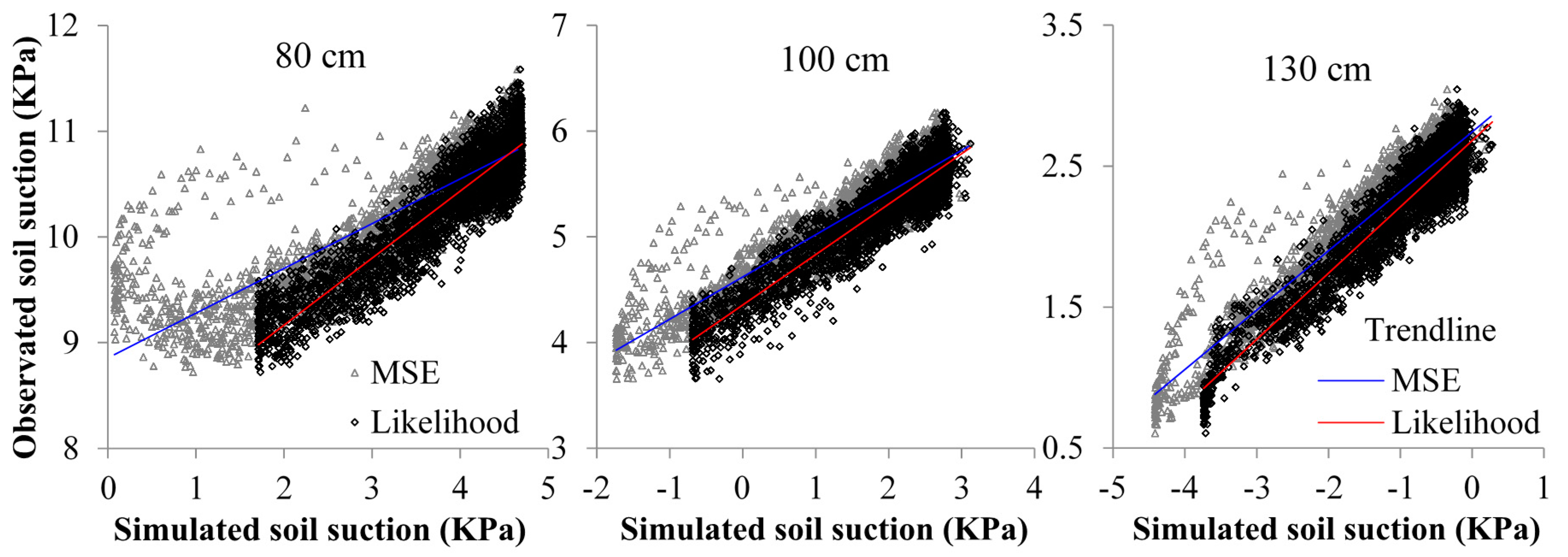
The groundwater levels and the soil suctions were used to validate the numerical groundwater model. Because of the limitations (such as the precision and the representation) of instruments and the scale effects, it is difficult to compare the measured values with the simulated values directly [3,4,6]. Therefore, a test of the linear relationship between observations and simulations was used to validate the model calibration results in this study. Figure 6 compares the observed and simulated soil suctions for the MSE and L methods in the first rainfall–runoff experiment. Correlation coefficient (R2) values of the L approach for 80, 100, and 130 cm depths are 0.845, 0.863, and 0.894, respectively. By contrast, R2 values of the MSE method for 80, 100, and 130 cm depths are 0.735, 0.849, and 0.876, respectively. R2 values of the L method are all much larger than those of the MSE approach, which means that MF2K-VSF with L can mimic the soil suctions better. Figure 6 also shows that there is an obvious hysteresis between the simulated soil suction of MF2K-VSF with MSE and the tensiometer measurements, which demonstrates large mismatch.
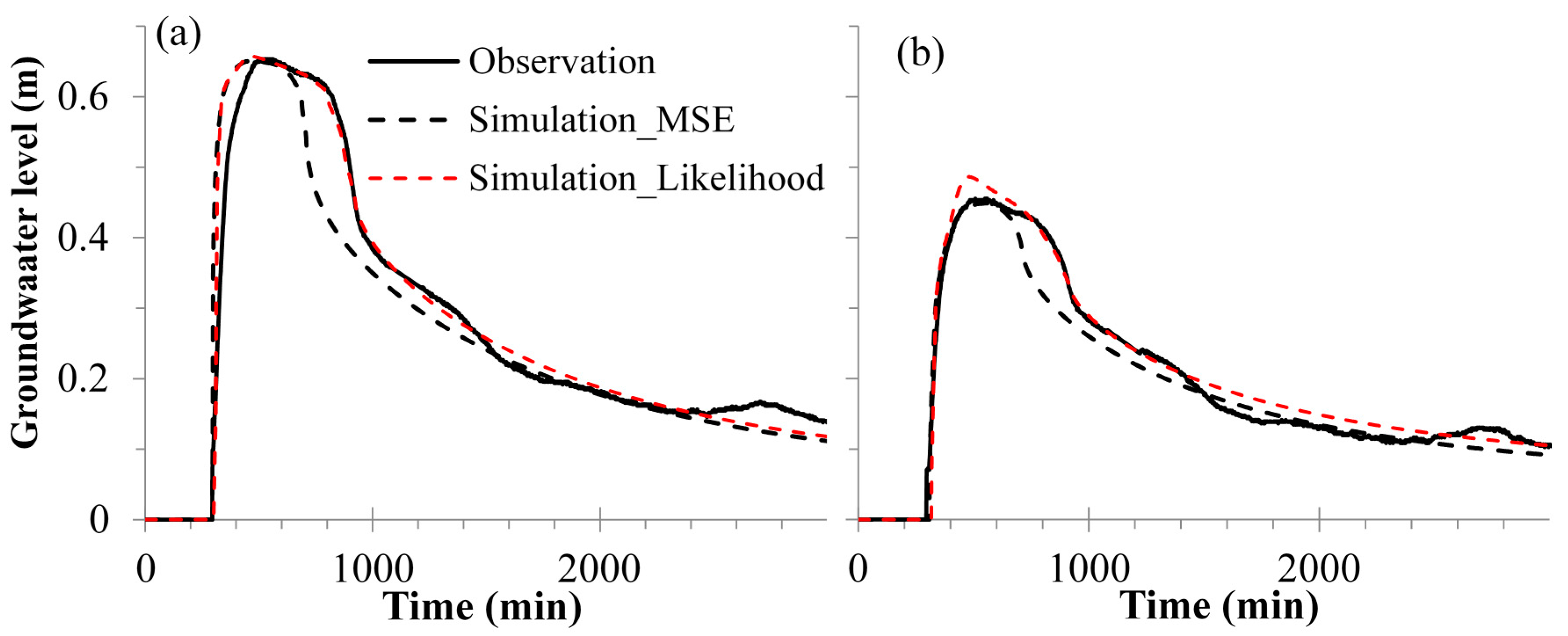
Comparison between the observed and simulated groundwater levels in the second rainfall–runoff experiment is shown in Figure 7. MSE values of simulated groundwater levels for MSE and L methods are 0.0021 and 0.0009 m2, respectively, which means that the numerical model with L can mimic the groundwater levels much better. Figure 7 also shows that the decline of groundwater level simulated by MF2K-VSF with MSE is significantly faster than that of observations.
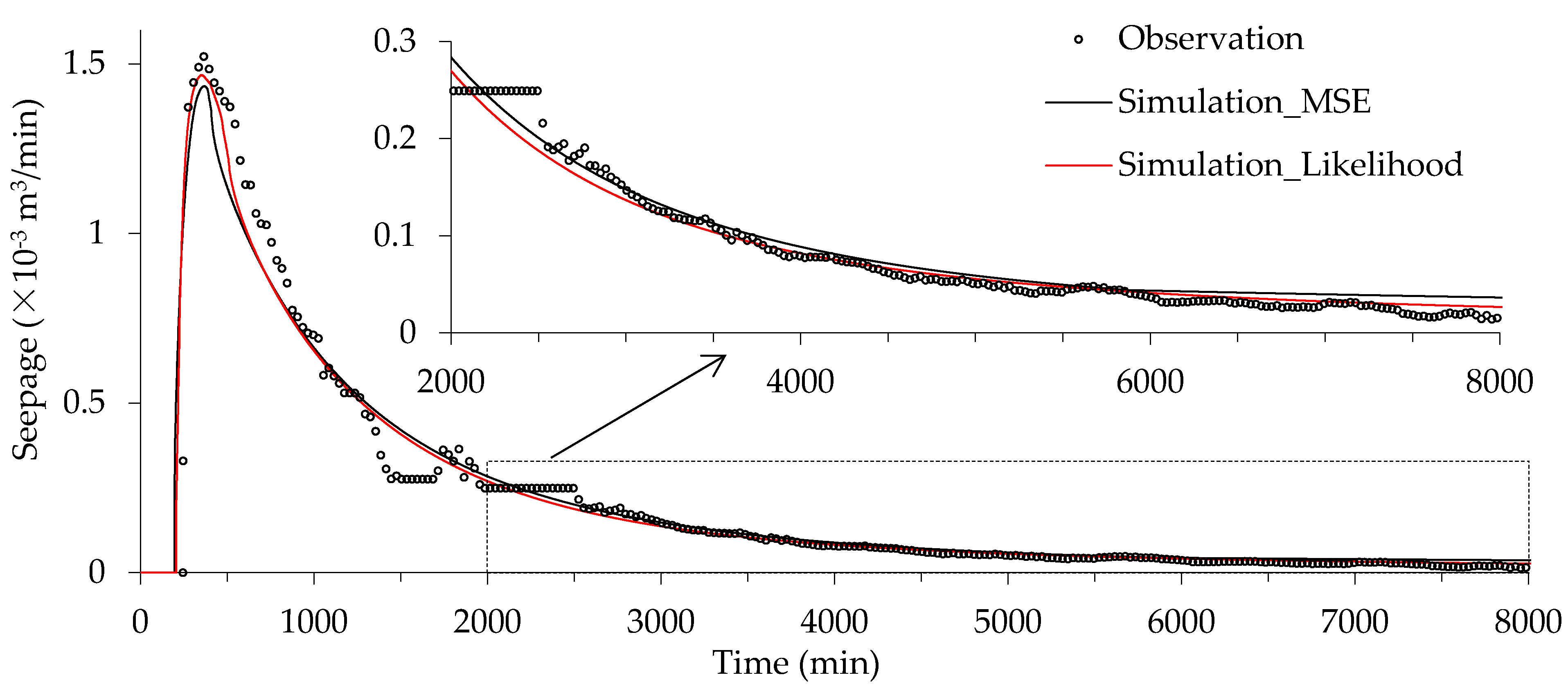
To verify the calibrated groundwater model, the optimal parameters given by the L and MSE criteria (Table 3) were used to simulate the third rainfall–runoff experiment. The simulated seepages are shown in Figure 8. The figure shows that using the optimal model parameters estimated with the L criterion, the simulated seepages are similar to those with the MSE criterion. Both of them can mimic the seepage recession processes well, but the mismatches around the peaks of simulated and observed seepages are relatively large, possibly because of increase of the observation errors as the observation was shifted to manual measurement.
Figure 9 compares the observed and simulated soil suctions at the depths of 80 and 100 cm in the third experiment. R2 values of the L approach for 80 and 100 cm depths are 0.828 and 0.843, respectively. By contrast, R2 values of the MSE method for 80 and 100 cm depths are 0.725 and 0.787, respectively. R2 values of the L method are all much larger than those of the MSE approach. Therefore, MF2K-VSF with L mimics the soil suctions much better than that with MSE. The hysteresis (i.e., noose curve) between the simulated and observed soil suctions reflects that the MF2K-VSF with MSE cannot well mimic both the wetting and drying processes.
In the noose curve, the upper part with sparse points belongs to the wetting period because the observed groundwater level recession (drying) period is much longer than its rising (wetting) period. The arrows in Figure 9 indicate the direction from wetting to drying. The direction of closed loop shows that during the wetting period, the change of simulated soil suctions is faster than that of observed soil suctions at the beginning, but later is slower. It demonstrates that the inverse modeling with MSE overestimates the percolation rate of soil water movement, but underestimates the drainage capacity of the filter layer; this is in agreement with the optimized parameter values in Table 3, where the Kv value for MSE method is greater than that for L approach, but the Kf value is less.
5. Discussions
MSE has become the standard efficiency criterion of inverse modeling to estimate soil property parameters, especially for the dynamics-based groundwater model [7,15,37]. However, many studies together with the results of this study show that inverse modeling with only the soil seepages/outflows cannot yield accurate model parameter estimates [6,38,39,40,41]. In theory (i.e., excluding any model inadequacy and input and observation errors), however, it is possible to obtain accurate estimates via inverse modeling [42]. Therefore, mistakes in inverse modeling may be caused by the efficiency criterion of MSE (Equation (11)) which neglects any inadequacies of the numerical groundwater model [15,29,43]. In our case study, the model structure errors are the main error sources of model residuals because of high autocorrelation (Figure 4c and Figure 5b), which clearly violates the statistical assumption of MSE. As a consequence, inverse modeling with MSE brings model structure errors into the optimized parameters, and ultimately concludes in fallacious results, such as the soil suctions (Figure 6 and Figure 9) and the groundwater levels (Figure 7) [14,15,21,29,43].
The model structure errors of our numerical model may mainly originate from the soil moisture hysteresis neglected by MF2K-VSF because the hysteresis effect is in general more pronounced in coarse-textured soil like that used in this study [44,45,46]. In general, the rate of soil wetting is greater than that of soil drying. Therefore, the soil hydraulic parameters (Equations (17) and (18)) of the wetting and drying processes are indeed different. Because the number of observed datapoints in the soil drying period is much greater than that in the soil wetting period in this study, the hydraulic parameters estimated by the inverse modeling primarily reflect those of the soil drying process (Figure 6 and Figure 9), which would underestimate the percolation rate of soil water in the soil wetting period [45,46]. Nevertheless, MSE neglects this deficiency of MF2K-VSF and attempts to reduce, to a great degree, these model structural errors. Therefore, the infiltration rate (e.g., the value of Kv in Table 3) is overestimated by MSE for capturing the seepages (especially at peak value) during the soil wetting period. As a result, the simulated groundwater levels by MF2K-VSF with MSE decay more rapidly than the observations (Figure 7) and the percolation rate of soil water is overestimated (Figure 6 and Figure 9). During the drying period, however, in order to reduce the adverse effect of the high percolation rate, the capacity of the soil water retention (drying) is overestimated slightly (Figure 3) and the drainage capacity (i.e., the value of Kf) of the filter layer is underestimated by MSE (Table 3; Figure 6 and Figure 9).
Compared with MSE, L separates the model structure and observation errors and removes the nonrandom components of model residuals via the AR(1) method. These operations weaken the effects of the model structural errors on the inverse modeling (Figure 5b,c). Therefore, the inverse modeling with L (Equation (14)) not only improves the optimized parameters (Figure 3), but also well mimics the groundwater levels (Figure 7) and soil suctions (Figure 6 and Figure 9).
In this study, the model residuals are mainly from the model structural errors while the observed errors can be neglected (Figure 4c and Figure 5b). As a result, the model calibration results of the L method are similar to those of the AR(1) approach. Therefore, the case study of soil tank rainfall–runoff experiments cannot be used to distinguish between the AR(1) and L methods. However, the structure of L is more reasonable than that of AR(1) (Equations (3) and (14) [30,32]). This study proves that AR(1) is only a special case of L in neglecting the observational errors. In the future, therefore, the effectiveness and robustness of L will need to be confirmed in continuous hydrograph modeling with low autocorrelation sequences, in contrast to the single-event hydrograph modeling in this study.
The L method separates the model structural and observational errors based on the separation of correlated and uncorrelated model residuals. In the soil tank rainfall–runoff experiments, because of the relatively homogeneous soil layer, the definite boundary conditions, and the stable initial state (which means input errors are negligible), the L approach can account for the correlation of model structural errors (Figure 5) and infer more reasonable results (Figure 3, Figure 6, Figure 7 and Figure 9). In real-world case studies (e.g., watershed modeling), however, because of the complex error sources of model residuals, such as correlated input and output measurement errors, L could fail to distinguish errors from model structure and observation. Additionally, L (Equation (14)) assumes that the model residuals are homoscedastic (i.e., have the same variance), while the model residuals in watershed models usually exhibit considerable heteroscedasticity (i.e., inconstant variance) owing to the large rainfalls and stream flows [24]. Therefore, it may be necessary to remove the heteroscedasticity of residuals (e.g., using the Box–Cox transformation method) before applying the L method [20,24,32].
6. Conclusions
Based on the idea of Reichert and Schuwirth [30], this study developed a practical formal likelihood function (L) to separate the model structural and observational errors under the assumptions that the model structural errors follow a multivariate Gaussian distribution and the observation errors follow a Gaussian distribution with a constant variance. Compared with the formal likelihood function proposed by Reichert and Schuwirth [30], L not only avoids calculating the inverse covariance matrix, but also combines the MSE and AR(1) methods. When the ratio between the variance of the random components of model structural errors and the variance of the model observational errors (b) equals 0, L is equivalent to MSE; when b approaches infinity, L approaches the AR(1) model. The case study of soil tank rainfall–runoff experiments shows that the performance of simulated seepages by MF2K-VSF with MSE is better than that with L, whereas the performance of the model validation using the groundwater levels and soil suctions and the new rainfall–runoff experiment is worse. The decomposition of model residuals by L reveals that the observation errors can be neglected, but the model structural errors are large and obviously auto-correlated. This may result from the model inadequacy of the numerical groundwater model (MF2K-VSF) owing to neglect of the hysteresis of the unsaturated soil water movement. The considerable model structure error clearly violates the statistical assumption of MSE and ultimately results in the fallacious inferences. By contrast, L reduces the effects of model structural errors. As a result, it improves reliability in the simulation of other hydrological components. Meanwhile, because of the negligible observational errors, the calibration results of the AR(1) approach are nearly the same as those of the L method.
The results of this study were obtained from a case study of simple soil tank rainfall–runoff experiments with a relatively homogeneous soil layer and accurate observations. For watershed modeling in the real world, because of the complex error sources of model residuals, such as correlated input and output measurement errors, whether L could be appropriately used for separating model structural and observational errors and increasing reliability in simulations still needs further investigation.
Author Contributions
Conceptualization & Methodology & Formal Analysis, Q.-B.C. and X.C.; Writing-Original Draft Preparation, Q.-B.C.; Sandbox Experiment & Writing-Review & Editing, D.-D.C., Y.-Y.W., and Y.-Y.X.
Funding
This research was funded by [National Natural Science Foundation of China] grant number [41601013, and 41571130071]; [Fundamental Research Funds for the Central Universities] grant number [2018B10714, and 2018B44714] and [Natural Science Foundation of Jiangsu Province, China] grant number [BK20150809].
Acknowledgments
We are grateful to Li-Li Zhao and Yu-Ying Liu for reviewing the English language. We would also like to thank three anonymous reviewers for their constructive comments that led to significant improvements to the paper.
Conflicts of Interest
The authors declare no conflicts of interest.
Appendix A. Analytical Solution of the Inverse Covariance Matrix
The matrix is equal to
We set Ak to be the matrix with dimension k:
We can obtain a recurrence formula to calculate the determinant of the matrix:
According to the Cramer law, the elements of the inverse matrix are
where is an element of the inverse matrix with dimension n, and i and j are the row and column numbers, respectively.
The elements of the inverse covariance matrix are
where is an element of the inverse covariance matrix with dimension n.
References
- Thoms, R.; Johnson, R.; Healy, R. User’s Guide to the Variably Saturated Flow (VSF) Process for MODFLOW; USGS: Reston, VA, USA, 2006.
- Twarakavi, N.K.C.; Simunek, J.; Seo, S. Evaluating Interactions between Groundwater and Vadose Zone Using the HYDRUS-Based Flow Package for MODFLOW. Vadose Zone J. 2008, 7, 757–768. [Google Scholar] [CrossRef]
- Vrugt, J.A.; Stauffer, P.H.; Wöhling, T.; Robinson, B.A.; Vesselinov, V.V. Inverse Modeling of Subsurface Flow and Transport Properties: A Review with New Developments. Vadose Zone J. 2008, 7, 843–864. [Google Scholar] [CrossRef]
- Laloy, E.; Fasbender, D.; Bielders, C.L. Parameter optimization and uncertainty analysis for plot-scale continuous modeling of runoff using a formal Bayesian approach. J. Hydrol. 2010, 380, 82–93. [Google Scholar] [CrossRef]
- Cheng, Q.; Chen, X.; Chen, X.; Zhang, Z.; Ling, M. Water infiltration underneath single-ring permeameters and hydraulic conductivity determination. J. Hydrol. 2011, 398, 135–143. [Google Scholar] [CrossRef]
- Zhou, H.; Gómez-Hernández, J.J.; Li, L. Inverse methods in hydrogeology: Evolution and recent trends. Adv. Water Resour. 2014, 63, 22–37. [Google Scholar] [CrossRef] [Green Version]
- Poeter, E.P.; Hill, M.C. Inverse models: A necessary next step in ground-water modeling. Groundwater 1997, 35, 250–260. [Google Scholar] [CrossRef]
- Green, I.; Stephenson, D. Criteria for comparison of single event models. Hydrol. Sci. J. 1986, 31, 395–411. [Google Scholar] [CrossRef] [Green Version]
- Legates, D.R.; McCabe, G.J., Jr. Evaluating the use of “goodness-of-fit” measures in hydrologic and hydroclimatic model validation. Water Resour. Res. 1999, 35, 233–241. [Google Scholar] [CrossRef]
- Krause, P.; Boyle, D.P.; Bäse, F. Comparison of different efficiency criteria for hydrological model assessment. Adv. Geosci. 2005, 5, 89–97. [Google Scholar] [CrossRef]
- Pushpalatha, R.; Perrin, C.; Le Moine, N.; Andréassian, V. A review of efficiency criteria suitable for evaluating low-flow simulations. J. Hydrol. 2012, 420, 171–182. [Google Scholar] [CrossRef]
- Bennett, N.D.; Croke, B.F.; Guariso, G.; Guillaume, J.H.; Hamilton, S.H.; Jakeman, A.J.; Marsili-Libelli, S.; Newham, L.T.; Norton, J.P.; Perrin, C. Characterising performance of environmental models. Environ. Model. Softw. 2013, 40, 1–20. [Google Scholar] [CrossRef]
- Nash, J.E. River flow forecasting through conceptual models, I: A discussion of principles. J. Hydrol. 1970, 10, 398–409. [Google Scholar] [CrossRef]
- Clarke, R.T. A review of some mathematical models used in hydrology, with observations on their calibration and use. J. Hydrol. 1973, 19, 1–20. [Google Scholar] [CrossRef]
- Vrugt, J.A.; Diks, C.G.H.; Gupta, H.V.; Bouten, W.; Verstraten, J.M. Improved treatment of uncertainty in hydrologic modeling: Combining the strengths of global optimization and data assimilation. Water Resour. Res. 2005, 41, 143–148. [Google Scholar] [CrossRef]
- Cheng, Q.; Chen, X.; Xu, C.; Zhang, Z.; Reinhardt-Imjela, C.; Schulte, A. Using maximum likelihood to derive various distance-based goodness-of-fit indicators for hydrologic modeling assessment. Stoch. Environ. Res. Risk Assess. 2018, 32, 949–966. [Google Scholar] [CrossRef]
- Neuman, S.P. Shlomo P. Neuman: A Brief Autobiography. Groundwater 2010, 46, 164–169. [Google Scholar] [CrossRef] [PubMed]
- Neuman, S.P.; Xue, L.; Ye, M.; Lu, D. Bayesian analysis of data-worth considering model and parameter uncertainties. Adv. Water Resour. 2015, 36, 75–85. [Google Scholar] [CrossRef]
- Tsai, T.C.; Yeh, W.G. Characterization and identification of aquifer heterogeneity with generalized parameterization and Bayesian estimation. Water Resour. Res. 2004, 40, 497–518. [Google Scholar] [CrossRef]
- Cheng, Q.; Chen, X.; Xu, C.; Reinhardt-Imjela, C.; Schulte, A. Improvement and comparison of likelihood functions for model calibration and parameter uncertainty analysis within a Markov chain Monte Carlo scheme. J. Hydrol. 2014, 519, 2202–2214. [Google Scholar] [CrossRef]
- Xu, C.Y. Statistical Analysis of Parameters and Residuals of a Conceptual Water Balance Model—Methodology and Case Study. Water Resour. Manag. 2001, 15, 75–92. [Google Scholar] [CrossRef]
- Stedinger, J.R.; Vogel, R.M.; Lee, S.U.; Batchelder, R. Appraisal of the generalized likelihood uncertainty estimation (GLUE) method. Water Resour. Res. 2008, 44, W00B06. [Google Scholar] [CrossRef]
- Beven, K.; Smith, P.; Westerberg, I.; Freer, J. Comment on “Pursuing the method of multiple working hypotheses for hydrological modeling” by P. Clark et al. Water Resour. Res. 2012, 48, W11801. [Google Scholar] [CrossRef]
- Evin, G.; Kavetski, D.; Thyer, M.; Kuczera, G. Pitfalls and improvements in the joint inference of heteroscedasticity and autocorrelation in hydrological model calibration. Water Resour. Res. 2013, 49, 4518–4524. [Google Scholar] [CrossRef] [Green Version]
- Yang, J.; Reichert, P.; Abbaspour, K.C. Bayesian uncertainty analysis in distributed hydrologic modeling: A case study in the Thur River basin (Switzerland). Water Resour. Res. 2007, 43, 145–151. [Google Scholar] [CrossRef]
- Schoups, G.; Vrugt, J.A. A formal likelihood function for parameter and predictive inference of hydrologic models with correlated, heteroscedastic, and non-Gaussian errors. Water Resour. Res. 2010, 46, W10531. [Google Scholar] [CrossRef]
- Li, L.; Xu, C.; Xia, J.; Engeland, K.; Reggiani, P. Uncertainty estimates by Bayesian method with likelihood of AR (1) plus Normal model and AR (1) plus Multi-Normal model in different time-scales hydrological models. J. Hydrol. 2011, 406, 54–65. [Google Scholar] [CrossRef]
- Reichert, P.; Mieleitner, J. Analyzing input and structural uncertainty of nonlinear dynamic models with stochastic, time-dependent parameters. Water Resour. Res. 2009, 45, W10402. [Google Scholar] [CrossRef]
- Doherty, J.; Welter, D. A short exploration of structural noise. Water Resour. Res. 2010, 46, W05525. [Google Scholar] [CrossRef]
- Reichert, P.; Schuwirth, N. Linking statistical bias description to multiobjective model calibration. Water Resour. Res. 2012, 48, 184–189. [Google Scholar] [CrossRef]
- Trefethen, L.N.; Bau, D. Numerical Linear Algebra; Society for Industrial and Applied Mathematics: Philadelphia, PA, USA, 1997. [Google Scholar]
- Honti, M.; Stamm, C.; Reichert, P. Integrated uncertainty assessment of discharge predictions with a statistical error model. Water Resour. Res. 2013, 49, 4866–4884. [Google Scholar] [CrossRef] [Green Version]
- Duan, Q. Global optimization for watershed model calibration. In Calibration of Watershed Models; Wiley: Hoboken, NJ, USA, 2003. [Google Scholar]
- Basilevsky, A. Applied Matrix Algebra in the Statistical Sciences; North-Holland: New York, NY, USA, 1983. [Google Scholar]
- Johnson, D.O.; Arriaga, F.J.; Lowery, B. Automation of a falling head permeameter for rapid determination of hydraulic conductivity of multiple samples. Soil Sci. Soc. Am. J. 2005, 69, 828–833. [Google Scholar] [CrossRef]
- Vrugt, J.A.; Braak, C.J.F.T.; Diks, C.G.H.; Robinson, B.A.; Hyman, J.M.; Higdon, D. Accelerating Markov Chain Monte Carlo Simulation by Differential Evolution with Self-Adaptive Randomized Subspace Sampling. Int. J. Nonlinear Sci. Numer. Simul. 2009, 10, 273–290. [Google Scholar] [CrossRef] [Green Version]
- Caldwell, T.G.; Wöhling, T.; Young, M.H.; Boyle, D.P.; McDonald, E.V. Characterizing disturbed desert soils using multiobjective parameter optimization. Vadose Zone J. 2013, 12, 2–23. [Google Scholar] [CrossRef]
- Kool, J.B.; Parker, J.C. Analysis of the inverse problem for transient unsaturated flow. Water Resour. Res. 1988, 24, 817–830. [Google Scholar] [CrossRef]
- Toorman, A.F.; Wierenga, P.J.; Hills, R.G. Parameter estimation of hydraulic properties from one-step outflow data. Water Resour. Res. 1992, 28, 3021–3028. [Google Scholar] [CrossRef]
- Eching, S.O.; Hopmans, J.W.; Wendroth, O. Unsaturated hydraulic conductivity from transient multistep outflow and soil water pressure data. Soil Sci. Soc. Am. J. 1994, 58, 687–695. [Google Scholar] [CrossRef]
- Inoue, M.; Šimunek, J.; Hopmans, J.W.; Clausnitzer, V. In situ estimation of soil hydraulic functions using a multistep soil-water extraction technique. Water Resour. Res. 1998, 34, 1035–1050. [Google Scholar] [CrossRef] [Green Version]
- Kool, J.B.; Parker, J.C.; Van Genuchten, M.T. Determining Soil Hydraulic Properties from One-step Outflow Experiments by Parameter Estimation: I. Theory and Numerical Studies 1. Soil Sci. Soc. Am. J. 1985, 49, 1348–1354. [Google Scholar] [CrossRef]
- Renard, B.; Kavetski, D.; Kuczera, G.; Thyer, M.; Franks, S.W. Understanding predictive uncertainty in hydrologic modeling: The challenge of identifying input and structural errors. Water Resour. Res. 2010, 46, W05521. [Google Scholar] [CrossRef]
- Hillel, D. Soil and Water: Physical Principles and Processes; Academic Press, Inc.: New York, NY, USA, 1971. [Google Scholar]
- Pham, H.Q.; Fredlund, D.G.; Barbour, S.L. A study of hysteresis models for soil-water characteristic curves. Can. Geotech. J. 2005, 42, 1548–1568. [Google Scholar] [CrossRef]
- McNamara, H. An estimate of energy dissipation due to soil-moisture hysteresis. Water Resour. Res. 2014, 50, 725–735. [Google Scholar] [CrossRef] [Green Version]
Figure 1.
Comparison between the synthetically generated data and the simulated results for model calibration criteria of mean squared error (MSE) and Likelihood.
Figure 1.
Comparison between the synthetically generated data and the simulated results for model calibration criteria of mean squared error (MSE) and Likelihood.

Figure 2.
Sketch of the rainfall–runoff experiment in the soil tank as well as the position of measuring instruments.
Figure 2.
Sketch of the rainfall–runoff experiment in the soil tank as well as the position of measuring instruments.

Figure 3.
Comparison of the soil water retention curve measured by the refrigerated centrifuge and estimated by the inverse modeling.
Figure 3.
Comparison of the soil water retention curve measured by the refrigerated centrifuge and estimated by the inverse modeling.

Figure 4.
Error analysis for the simulated seepages of the MSE method. (a) Comparison between the observed and simulated soil tank seepages. (b) Errors between the observed and simulated seepages. (c) Partial autocorrelation coefficients of errors with 95% significance levels. Left column is for the first experiment and right column is for the second experiment.

Figure 5.
Error analysis for the simulated seepages of the practical formal likelihood function (L) method. (a) Comparison between the observed and simulated soil tank seepages. (b) Decomposition of the model residuals into model structural and observational errors. (c) Partial autocorrelation coefficients of model structural errors after AR(1). Left column is for the first experiment and right column is for the second experiment.

Figure 6.
The observation soil suctions versus the simulations at the depths of 80, 100, and 130 cm in the first rainfall–runoff experiment. Note that the positive value of soil suction means that soil is unsaturated, rather than saturated, which is opposite to the value of the water pressure head.
Figure 6.
The observation soil suctions versus the simulations at the depths of 80, 100, and 130 cm in the first rainfall–runoff experiment. Note that the positive value of soil suction means that soil is unsaturated, rather than saturated, which is opposite to the value of the water pressure head.

Figure 7.
Comparison between the observed groundwater levels and simulated groundwater levels in the second rainfall–runoff experiment at (a) observation well 1 and (b) observation well 2.
Figure 7.
Comparison between the observed groundwater levels and simulated groundwater levels in the second rainfall–runoff experiment at (a) observation well 1 and (b) observation well 2.

Figure 8.
Comparison between observed and simulated soil tank seepages in the third rainfall–runoff experiment for model validation.
Figure 8.
Comparison between observed and simulated soil tank seepages in the third rainfall–runoff experiment for model validation.

Figure 9.
The observed soil suctions versus the simulations at the depths of 80 and 100 cm in the third rainfall–runoff experiment.
Figure 9.
The observed soil suctions versus the simulations at the depths of 80 and 100 cm in the third rainfall–runoff experiment.


Table 1.
Comparison of the runtime of the analytical solution and inverse matrix approach.
| Number of Observation Datapoints | 3142 | 6283 | 9424 | 12,565 | 15,706 | |
|---|---|---|---|---|---|---|
| Runtime (s) | Analytical Method | 1.71 | 3.01 | 5.61 | 9.33 | 13.84 |
| Matrix Inversion | 30.83 | 518.6 | 2712.48 | Out of memory | ||
Table 2.
Optimized results of model parameter values and corresponding criterion values of MSE and Likelihood.
Table 2.
Optimized results of model parameter values and corresponding criterion values of MSE and Likelihood.
| Model Parameter | y = sin(c × x + d) | Criterion Values | ||
|---|---|---|---|---|
| c | d | (min) MSE | (max) Likelihood | |
| Synthetic data | 1.000 | 0.000 | 0.0178 | 53.444 |
| MSE | 0.940 | 0.149 | 0.0137 | 51.749 |
| AR(1) a | 1.021 | −0.007 | 0.0189 | 53.683 |
| Likelihood | 1.016 | 0.005 | 0.0182 | 53.696 |
a First-order autoregression.
Table 3.
Description of model parameters with measured values and optimized results.
| Parameters a | Definition | Measured | Calibration Result | |||
|---|---|---|---|---|---|---|
| MSE | AR(1) | Likelihood | ||||
| Kh | Horizontal soil hydraulic conductivity (×10−5 m/s) | ― | 8.927 | 0.287 | 0.301 | |
| Kv | Vertical soil hydraulic conductivity (×10−6 m/s) | 6.884 | 5.148 | 4.884 | 4.899 | |
| α1 | α for unsaturated hydraulic conductivity (1/m) | ― | 1.905 | 2.129 | 2.130 | |
| n1 | n for unsaturated hydraulic conductivity | ― | 6.265 | 5.247 | 5.247 | |
| α2 | α for soil water retention (1/m) | 2.319 | 1.408 | 1.502 | 1.503 | |
| n2 | n for soil water retention | 2.686 | 3.264 | 3.062 | 3.062 | |
| Kf | Hydraulic conductivity of filter layer (×10−3 m/s) | ― | 1.558 | 2.903 | 2.903 | |
| Error model | R | Autocorrelation coefficient | ― | ― | 0.9954 | 0.9996 |
| b | Ratio between the variance of model structure and observation errors | ― | ― | ― | 3.02 | |
| Criteria | (min) MSE | 0.00088 | 0.00172 | 0.001691 | ||
| (max) Likelihood | 39,828 | 40,562 | 40,593 | |||
a Dual set of parameters used in the van Genuchten–Mualem (VGM) functions.
© 2018 by the authors. Licensee MDPI, Basel, Switzerland. This article is an open access article distributed under the terms and conditions of the Creative Commons Attribution (CC BY) license (http://creativecommons.org/licenses/by/4.0/).
Share and Cite
MDPI and ACS Style
Cheng, Q.-B.; Chen, X.; Cheng, D.-D.; Wu, Y.-Y.; Xie, Y.-Y. Improved Inverse Modeling by Separating Model Structural and Observational Errors. Water 2018, 10, 1151. https://doi.org/10.3390/w10091151
AMA Style
Cheng Q-B, Chen X, Cheng D-D, Wu Y-Y, Xie Y-Y. Improved Inverse Modeling by Separating Model Structural and Observational Errors. Water. 2018; 10(9):1151. https://doi.org/10.3390/w10091151
Chicago/Turabian StyleCheng, Qin-Bo, Xi Chen, Dan-Dan Cheng, Yan-Yan Wu, and Yong-Yu Xie. 2018. "Improved Inverse Modeling by Separating Model Structural and Observational Errors" Water 10, no. 9: 1151. https://doi.org/10.3390/w10091151
Note that from the first issue of 2016, this journal uses article numbers instead of page numbers. See further details here.