Considering Abrupt Change in Rainfall for Flood Season Division: A Case Study of the Zhangjia Zhuang Reservoir, Based on a New Model

Department of Groundwater Resources and Environment, College of Water Science and Engineering, Taiyuan University of Technology, Taiyuan 030024, China
*
Author to whom correspondence should be addressed.
Water 2018, 10(9), 1152; https://doi.org/10.3390/w10091152
Submission received: 8 August 2018
/
Revised: 20 August 2018
/
Accepted: 26 August 2018
/
Published: 28 August 2018
(This article belongs to the Section Water Use and Scarcity)
Abstract
:The traditional flood season division method is cumbersome. In order to make the flood season division elaborate, the Mann–Kendall and cumulative sum of rank difference (CSD) methods were used to detect the abrupt change year of precipitation (p) over the study area from 1969 to 2015. The year of change was determined to be 1995. Taking the 1995 year as a demarcation point of the data, the discriminant model and Fisher optimal partition method were applied for flood division, and a comparison of the results from the two approaches were compared. The discriminant model was found to perform slightly better than the Fisher approach. It was found that abrupt rainfall change has a certain influence on flood season division. The main flood season in the Zhangjia Zhuang reservoir during 1969–2015 was 16 days longer than during 1996–2015, but three days shorter than between 1969–1995. For the Zhangjia Zhuang Reservoir, the flood water level limit can increase up to 2 m according to the results of the flood season division and designed rainfall after abrupt change; in addition, the water storage capacity is 469 million m³ more than that of the traditional reservoir operation mode.
1. Introduction
Rainstorms and floods are more distinct from one another during different periods, and the flood season is divided into several periods, on the basis of accounting for the law of this difference [1]. In practical work, it is of great significance to rationally determine the stages of the flood season, which is the precondition for reservoir flood control, and is of great significance to the rational application of flood control and water resources in the basin and reservoir [2]. In the past, the long series of rainfall and runoff data have often been used to divide the flood season, and factors such as climate change and extreme weather were not considered [3]. A large number of studies show that the trend of global warming is remarkable in the past hundred years. The Intergovernmental Panel on Climate Change assessment report affirmed the objective facts of climate warming, and pointed out that the increase of temperature will affect many natural systems [4]. Climate change is a global issue that impacts every living being in the world. One of the most noticeable consequences of this global phenomenon is the inevitable water cycle modification, with precipitation being a major component in these processes [5]. Several studies have investigated the duration of flood seasons. Odekunle [6] determined rainy season onset and retreat over Nigeria by two kinds of rain indices, and suggests that is better to use number of rainy days than rainfall amount. Sâmia et al. [7] proposed an effective method to detect the occurrence and extinction date of rainy seasons in some parts of South America. Wang et al. [3] studied the duration and division of the flood season in the Fenhe River Basin, and found that climate change has a great influence on the node of the flood season, the main flood season after the climate change has been shortened. Hachigonta et al. [8] investigated the onset and cessation dates of the main summer rainy season over Zambia, and found that the onset date of the flood season in Zambia has a significant spatial variation. Other studies [9,10,11,12,13] have analyzed temporal variations in flood seasons. All these studies show that climate change has a significant impact on the time node changes during the flood season, but there are few studies on the effects of climate change on the division and operation of the reservoir during the flood season. Climate change affects the global hydrological cycle, causing significant changes in time and space. During the operation of the reservoir, the change of precipitation and other factors caused by climate change will affect the change of the time points in the flood season. In the new period and new situation, it is necessary to change the traditional idea of the flood season division, and consider the impact of climate change on flood season staging and reservoir operation.
Because of flood season randomness, certainty, and fuzziness, the flood season division method is varied according to its characteristics. The current flood season staging methods mainly include the change point analysis method [14], fuzzy set analysis method [15], system clustering method [16], and Fisher most segmentation method [17]. These methods have shortcomings, such as single selection index or cumbersome calculation. Neither can provide simple and reasonable flood season staging [18,19]. The flood season division is a state of quantitative-qualitative change cycle: quantitative changes continued over a period of time in the pre-flood season, then qualitative changes to the main flood season; quantitative change continues over a period time during main flood season, then qualitative changes to the post-flood season. The changing process of flood seasons conforms to the theoretical basis of quantitative-qualitative change of variable sets.
Considered the existing problems in the current stage of flood season divisions, this paper launches the following research: (1) based on the variable set theory, a new method of flood season division, using some mathematical concepts and functions, is proposed. (2) Taking the precipitation catastrophe point of Zhangjia Zhuang reservoir as the dividing point, the discriminant model and the Fisher optimal segmentation method are used to divide the flood season of Zhangjia Zhuang reservoir before and after the catastrophe point. (3) Establish the evaluation index of the result of the flood season division result; then, the rationality and accuracy of the method are verified by using the index to compare the model flood season division result with the Fisher optimal segmentation method result. (4) The operation of Zhangjia Zhuang reservoir was researched according to the standard of the traditional flood season division results and the flood season division results after the climate change year, respectively.
2. Materials and Methods
2.1. New Technique
2.1.1. Opposite Difference Function
Make when , , , , , and . is the opposition difference, or opposite difference function, that relates to and . Mapping , is called the opposite difference function between and .
2.1.2. Variable Set
Make
where is called the variable set; are called the main domain, main domain, gradual metamorphic boundary, and abrupt qualitative metamorphosis of variable set , respectively [20].
2.1.3. Discriminant Model Based on Variable Set
Let act as an opposite difference function for any element in discourse domain to . Change to before changing ; after the change of , the opposite relative membership functions are and , and the opposite difference function is . The discriminative modes of quantitative and qualitative change (gradual change and abrupt form) are as follows:
If , it means a quantitative change .
If , it means a gradual qualitative change (through ).
2.2. Application of the New Method Based on the Technique
Set and as the opposite and vague concepts of the pre-flood season and the main flood season (or the post-flood season and the main flood season). and represent the relative membership degree of to and ; in addition, , , and , Considering the time series, the transition from the pre-flood season to the main flood season and the ranges from 0 to 1 to 0, and the transition from the main flood season to the post-flood season and ranges from 1 to 0 to 1. The concrete steps are as follows:
Step 1: construct matrix X of index eigenvalue:
where is the characteristic value of time series and index .
Step 2: obtain the normalization matrix X1 by dimensionless X of the eigenvalue matrix.
Step 3: according to the normalized matrix X1, we can get the time series of composite index.
Set a known index in weight vector . Let any characteristic value of time Series as index , between and .
The multiple-index generalized distance of to the is
where P is distance parameter, P = 1 means Hamming distance, P = 2 means Euclidean distance.
The multiple index generalized distance of to the is:
The generalized distance of the synthetic index is optimized and transformed into a set of time series , and is the sequential eigenvalue of the composite indices.
According to Equations (2) and (3), Equation (4) can be changed into
where α is optimization criteria parameter. α = 1 means a minimum one square optimization criterion, and α = 2 means optimization criteria has a minimum of two squares. Considering that α = 2 has an amplification or reduction effect on distance, in the application of flood season division, α = 1 is selected.
If α = 1, P = 1, at this time the sequence of the comprehensive index is X11, then the Equation (5) becomes a linear formula:
If the flood season division is a nonlinear system, it can make P = 2. Under this circumstance, the sequence of the comprehensive index is X12, and Equation (5) can be changed to
Step 4: Determine the interval matrix of the standard value of , which means that the characteristic value of the comprehensive index sequential sequence X11 and X12 falls into the pre-flood season, and the main flood or main and post-flood seasons’ relative degrees of membership is 1; according to the known matrix X11 and X12, the standard interval matrix Y can be obtained:
where represent the largest and minimum eigenvalues of time series .
Step 5: Calculate the relative membership degree of index of sequences X11 and X12 for falling into the interval, respectively:
Step 6: Calculate the average relative membership degree of in two cases—X11 and X12.
Step 7: Calculate the average opposition difference degree of to :
where , and when , , which means there is a gradual qualitative change point.
Step 8: Analysis the evolution rule of flood season by discriminant models:
If , there is quantitative change.
If , there is gradual qualitative change, means the evolution of the flood season has crossed the gradual qualitative change boundary—that is, from the pre-flood season to the main flood season, or from the main flood season to the post-flood season.
2.3. Abrupt Change over a Year of Rainfall
The Mann–Kendall test (Mann 1945; Kendall 1975) is a nonparametric trend testing approach. It was modified to monitor changes over time. The modified version is called the sequential Mann–Kendall (MK) test [21,22], and it is applied in many studies (for instance, see [21,22,23,24,25,26]). The cumulative sum of rank difference (CSD) trend test makes use of both graphical diagnoses and statistical analyses, which were recently developed by Charles Onyutha [27,28,29], and is well applied to assess changes in the hydrometeorology [30] (see, for instance, [27,28,29]). However, the differences between the two methods are not negligible when applied in order to detect trends in a time series with persistent fluctuations. In trend analyses, the use of one method leads to uncertainty in the results, due to the influence from the choice of the method. Therefore, CSD and MK tests were adopted in this paper.
2.4. Fisher Optimal Segmentation Method
The Fisher optimal segmentation method is used as a method of clustering the sequence of ordered time samples, which is based on the minimum square sum of the sample total deviation, with the smallest difference within the class and the maximum difference between the classes. The Fisher optimal partition method wan used to divide the seismicity period and the flood season period [31]. The instalment of the flood season belongs to cluster analysis, and the cluster analysis is divided into ordered sample cluster analysis and non-ordered sample clustering analysis. Fisher optimal segmentation is used as a clustering method for ordered samples, which makes the Fisher optimal segmentation method widely used for the flood season. Therefore, the Fisher optimal partition method is applied in this paper to divide the flood season of the Zhangjia Zhuang reservoir. The specific steps of Fisher detection are then further explored [3].
2.5. Evaluation Index of Flood Season Division Results
In the past, the study of flood season staging has mostly used various theoretical methods, and the evaluation of the results of the division is rarely involved. This is because the physical causes of flood season are complex and changeable, so it is difficult to establish a physical model that directly reflects the nature of division. On the other hand, this is because the discriminant index system of the division results has not yet been established, and it is still impossible to make a scientific and reasonable evaluation for the results obtained. A series of mean square deviation can reflect the relative concentration or dispersion of each series of samples; the essence of flood season division is to divide a long series into several centralized short series with relatively identical sample characteristics, and the main flood season is more important than the pre-flood season or the post-flood season, and is the key period for reservoir operation. Therefore, different weights can be assigned to different stages of flood season, and the weight of the main flood season is relatively large. Based on the above theory, the evaluation index of mean square error S that considers the weight factor is proposed in this study. The evaluation index S can be expressed in the following steps.
Step 1: Let be the number of samples (the number of years); xi,j are selected as the index of the test results (generally selected daily rainfall), is the number of days in flood season, and is the number of years in flood season., if mk is the length of the K staging period (days), and mk+1 is the length of the K + 1 staging period (days). When n = 1, it means that there is only one research year, and the standard deviation S of each division at n = 1 can be expressed as:
Step 2: Let equal the number of staging points; is the number of divisions, K is the time period of the flood season, and λk is the weight factor corresponding to the k phased period, which can be set according to the bias of different divisions. The standard deviation of one year can be expressed as
Step 3: When the research period lasts for many years, the evaluate index S can be expressed in the following form:
2.6. Case Study Area
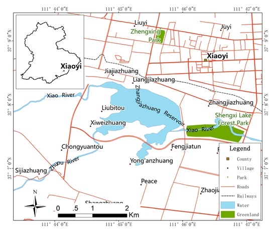
The Zhangjia Zhuang reservoir, located in the Yellow River Basin, is located in the south of the new city in Xiaoyi, Shanxi Province, China. It is a medium-sized reservoir on the main stream of the Fenhe River system and the main stream of the Xiao River. It has comprehensive benefits of flood control, agricultural irrigation, and ecological water supply. According to the reservoir basic data statistics, from 1963 to the end of 2013 (51 years), the reservoir downstream irrigation reached a total of 299.87 million m3, with a total irrigation area of 71,500 million m2. The location of Zhangjia Zhuang reservoir is shown in Figure 1.
3. Results
3.1. Temporal Distribution of Rainfall
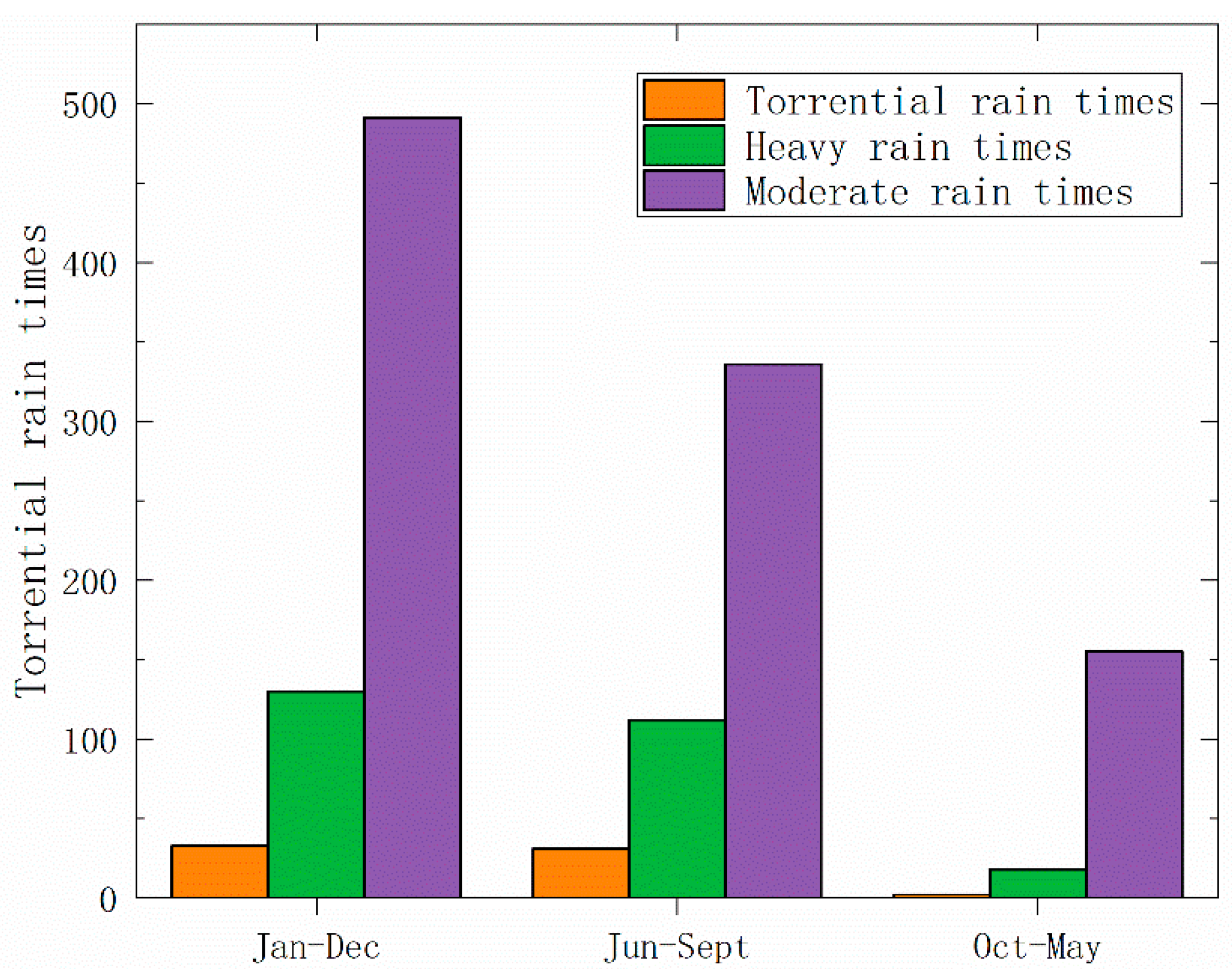
The precipitation data are mainly used from 47 years from 1969 to 2015. The daily precipitation data of Zhangjia Zhuang Reservoir from June to September are analyzed in detail. The results of the statistical analysis are shown in Figure 2. In these 47 years, rainfall (daily rainfall ≥ 10 mm), heavy rain (daily rainfall ≥ 25 mm), and rainstorms (daily rainfall ≥ 50 mm) occurred 491, 130, and 33 times, respectively; these instances occurred 336, 112, and 31 times from June to September, respectively, accounting for 68%, 86%, and 94% of the total number for each rainfall level. It can be seen that the precipitation in this study area is mainly concentrated in the period from June to September.
3.2. Abrupt Change over a Year of Rainfall
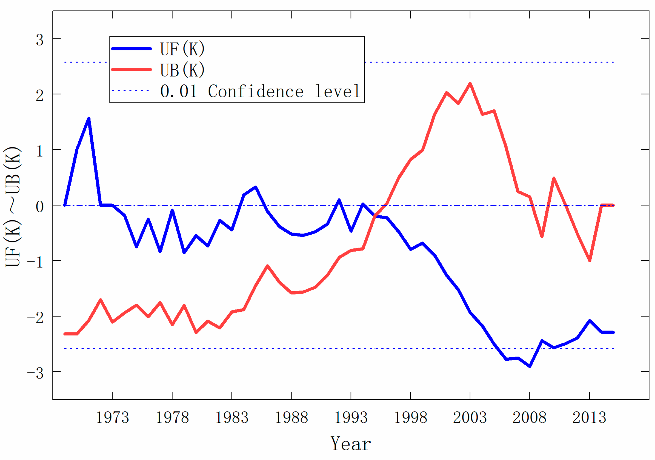
The annual precipitation during the 1969–2015 results by Mann–Kendall detection is shown in Figure 3. UF(K) and UB(K) are statistics sequence that obey standard normal distribution. An intersection exists between the UF(K) line and UB(K) line, which lies just between the two critical lines, whose confidence level is 0.01. The corresponding time of the intersection is 1995. Therefore, we can divide the period 1969–2015 into two periods, namely 1969–1995 and 1996–2015. The annual precipitation is on the rise during the former period, while the trend declines during the latter period.
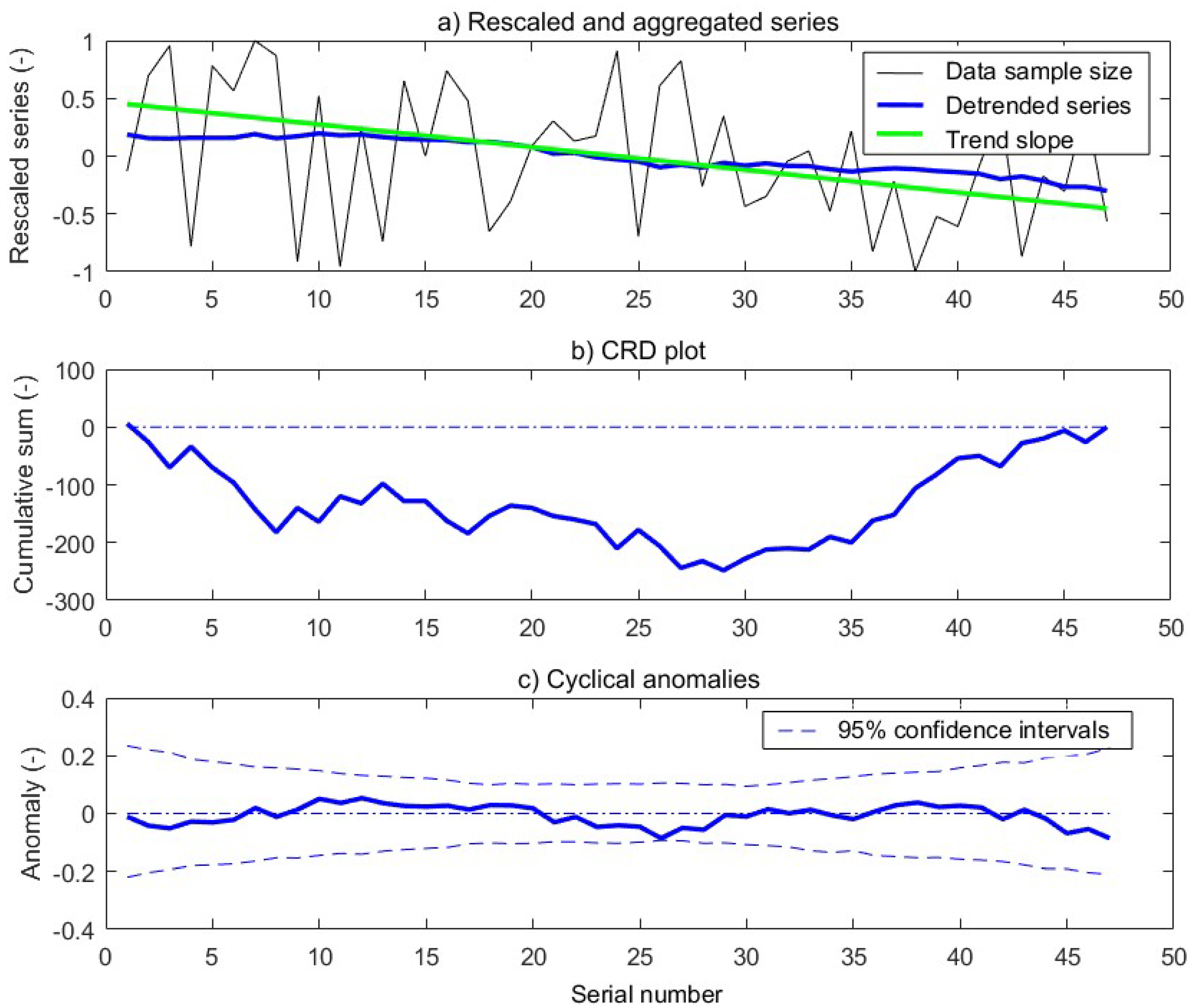
The annual precipitation during 1969–2015 results by CSD test is shown in Figure 4, where the line showing a cumulative sum of 0 is taken as the reference. The deviation of the values of the cumulative sum from the reference characterizes temporal changes in the series. For a time series with a sub-period characterized by a random variation of the values, while in the other part there is a linear trend, the tendency to form a curve will be obtained over the section with the linear trend [29]. Therefore, from Figure 4a,b, where the trends of rainfall can reach a serial number between 0–25, the series characterized by random variation but between serial numbers 26–50 are characterized by a linear decreasing trend, which corresponds to the tendency to form a curve between 26–50 in Figure 4b. For a series that has no trend in the first part, but a linear increase or decrease in the second portion, the change point is where the curve over the last sub-period begins [29]. As a result, we can get the change point from Figure 4b, in which the serial number 26 corresponds with the biggest anomaly in Figure 4c (also serial number 26). Therefore, we can observe that the precipitation changed regular from 1969 to 2015; in addition, there is a random trend from 1969 to 1994, and a current decreasing trend from 1995 to 2015. The abrupt change point of precipitation was 1995, which is consistent with the MK test results. In this paper, then, we regard 1995 as the abrupt change point of rainfall in the region.
3.3. Flood Season Division Results
3.3.1. Division by Discriminant Model
From the above analysis, we can get June to September as the research period for the flood season. The whole flood season period is divided into 12 segments consisting of 10-day periods. Four factors that can represent the seasonal rules of precipitation and floods were chosen as the basis elements for flood season division: the annual average 10-day rainfall, the annual average 10-day maximum one-day rainfall, the annual average 10-day maximum three-day rainfall, and rainstorm days (the daily rainfall is more than 25 mm). In the 1969–2015, 1969–1995, and 1996–2015 flood seasons, the characteristic value matrixes of rainstorm index are X1, X2, and X3, respectively.
Take the 1969–2015 characteristic matrix as an example, according to the matrix X1, and Equations (1)–(8) get two standard interval matrices, which are are as follows:
According to Equation (9), the relative degree of membership under linear model and nonlinear model can be obtained:
The average relative superior degree is as follows:
The mean opposite difference is as follows:
The discriminant model is used to analyze the evolution process of the flood season based on comprehensive indicators, as follows. Regard the first 10 days of June as the beginning; from this beginning to the third 10 days of June, , meaning that the comprehensive index is the quantitative change in this period. From the third 10 days of June to the first 10 days of July, , which shows that the comprehensive index has changed gradually to qualitative, which indicates that the change of the rainfall index has crossed the gradient boundary; in other words, it shows evolution of the flood season transition from the pre-flood to the main flood season. From the first 10 days of July to the first 10 days of September,, meaning that the comprehensive index is the quantitative change in this period. From the third 10 days of September to the second 10 days of September, , which shows that the comprehensive index has gradually become qualitative, demonstrating that the change of the rainfall index has crossed the gradual change boundary, and the evolution of flood season has changed from the main to the post-flood season. From the second 10 days of September to the third 10 days of September, , meaning that the comprehensive index is the quantitative change in this period.
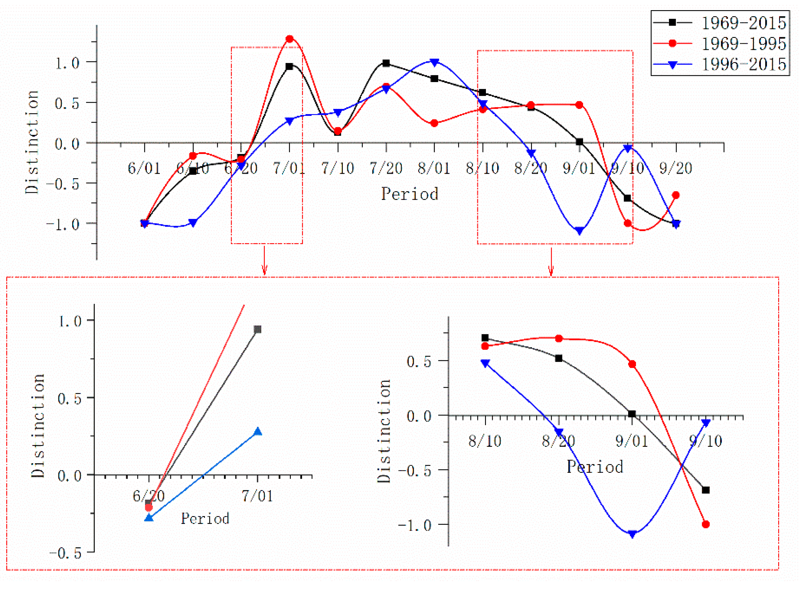
In the same analysis, the average opposition difference degree in the time series from the 1969–1995 and 1996–2015 rainfall indices obtained from X2 and X3 is shown in Figure 5. The results of the 1969–2015, 1969–1995, and 1996–2015 pre-flood season, main flood season, and post-flood season can be seen in Table 1.
3.3.2. Division by Fisher
Table 2, Table 3 and Table 4 display the results of the division of the periods 1969–2015, 1969–1995, and 1996–2015, respectively. Figure 6 shows the B (n, k)-k curve and f (k)-k curves of 1969–2015, 1969–1995, and 1996–2015, respectively. The f (k) is the maximum when k is equal to 3 in., and the curve B (n, k)-k has a turning point at the same time. Therefore, the optimal division number k is 3 during 1969–2015, 1969–1995, and 1996–2015, which means the flood season can be divided into three stages during 1969–2015, 1969–1995, and 1996–2015—namely a pre-flood season, main flood season, and post-flood season. The corresponding classification in Table 2, Table 3 and Table 4 are 1–4, 5–9, and 10–12, which means the pre-flood season is from 1 June to 10 July, the main flood season is from 11 July to 30 August, and the post-flood season is from 1 September to 30 September. The division of the flood season is consistent between the different research periods, and the results were not affected by the study period.
3.3.3. Evaluation and Comparison of Division Results
The daily rainfall of the 1969–2015 flood periods (6.01–9.30) for the Zhangjia Zhuang reservoir was selected as the characteristic index of the reservoir in the flood season. Using Equation (13), under the combination of three different weights, the discriminant model and the Fisher method were obtained for the evaluation index S for different divisions of the flood season. The results are shown in Table 5.
It is known from Table 5 that the mean variance of each stage and the S-Model under the three groups of different weight factors were smaller than the corresponding indices of the Fisher method. The results show that the results of the flood season division obtained by the discriminant model can better reflect the actual situation, and be more detailed and reasonable. Therefore, in this paper, the results of flood season division obtained by the discriminant model were selected to study the influence of the changes of time nodes in the flood season on reservoir operation. In addition, the S calculated by the two methods from 1996–2015 was less than from 1969–2015, which indicates that division in 1996–2015 was closer to the reality than for 1969–2015, so it is necessary to consider changes in the spatial and temporal distribution of rainfall during the period of the flood season.
3.4. Reappearance Period Rainfall Design and Reservoir Operation
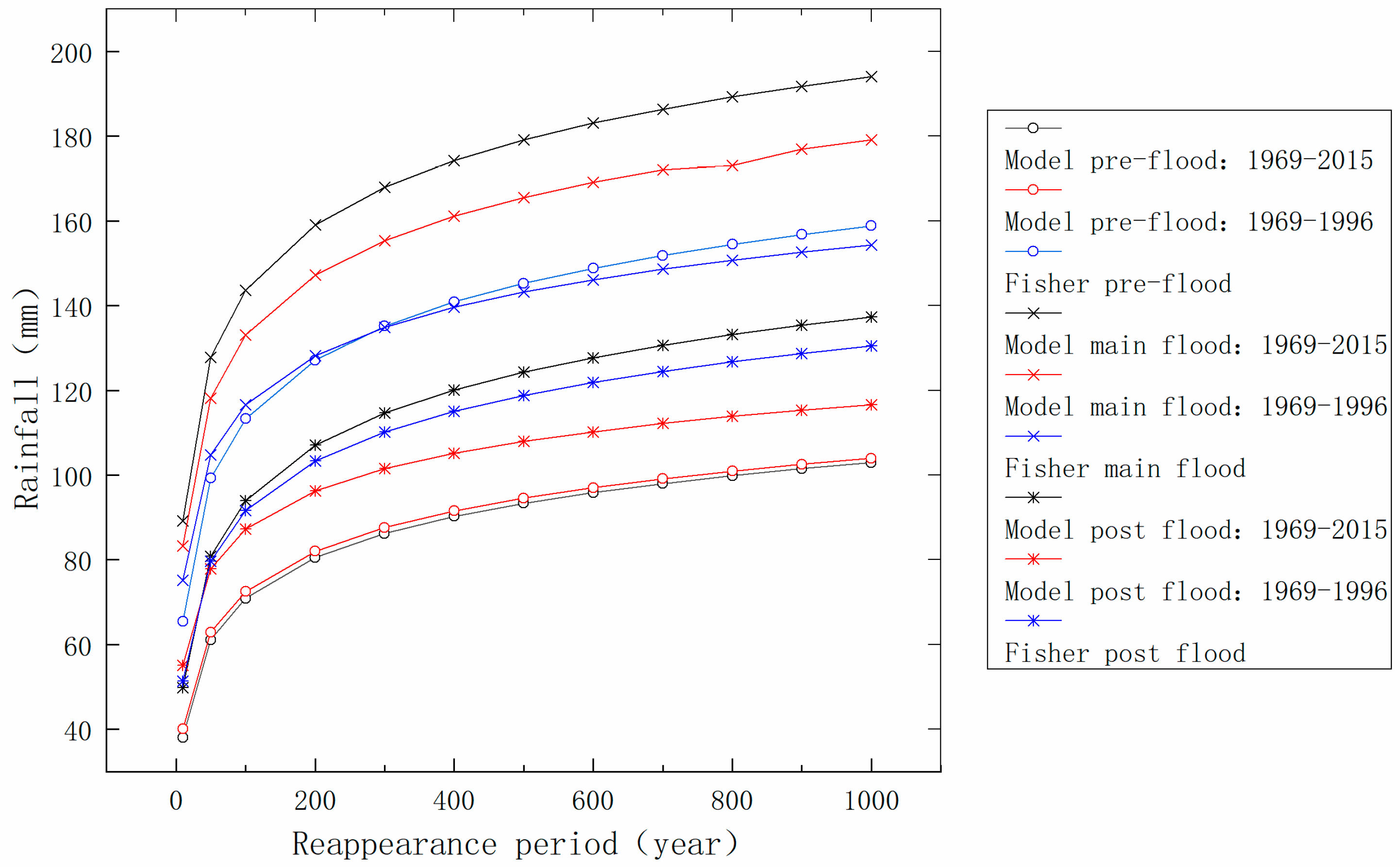
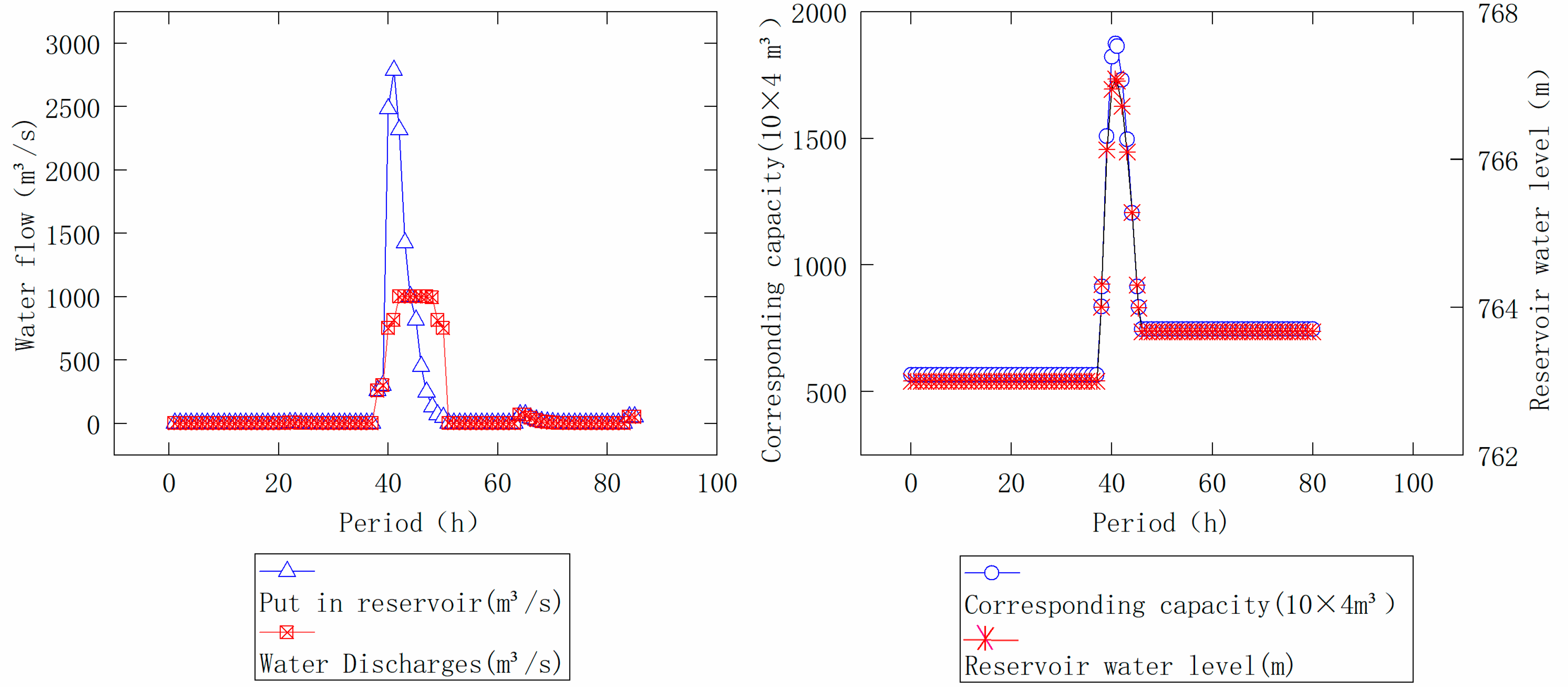
The important purpose of constructing the extreme value model is to study the recurrence level of extreme events. In hydrologic calculation, hydrologic experience frequency analysis, especially Pearson III distribution, is always used. In this paper, the Pearson III distribution is used to explore the recurrence characteristics of the peak value of the rainfall stage in the Zhangjia Zhuang reservoir. The extreme rainfall design values under different division results from 10–1000 are shown in Figure 7. Firstly, from the reliability analysis of the two methods, it can be seen that Fisher has the highest design rainfall for the pre-flood period and the lowest design rainfall for the main flood season. This is not conducive to the benefit of the reservoir or to the reservoir flood control. Therefore, the results of the model are more reasonable in the practical application. Secondly, from the point of view of the influence of abrupt change in rainfall mean on the division of reservoir flood season, the pre-, main, and post-flood period of the design rainfall mean after an abrupt change is less than for the whole period of time. This is consistent with the decreasing trend of rainfall in the Zhangjia Zhuang reservoir. Looking at the benefits, the design rainfall in the flood season after the abrupt change in mean is low—the corresponding reservoir flood limit water level could be higher, the reservoir water storage could be more, and it is more conducive to the rational use of water resources. Therefore, the design level of rainfall after an abrupt change in mean as the standard can raise the flood limit water level. The current flood limit water level in Zhangjia Zhuang reservoir was 762.0 m in the main flood season, 764.0 m in the later flood season, and the allowed checking flood level for extreme high water is 766.36 m. In this paper, the flood limit water level of Zhangjia Zhuang reservoir during the main flood season was raised to 764.0 m, and the flood routing (p = 0.1%) was checked to obtain the highest level of flood regulation and to verify the possibility of raising the flood limit water level of the reservoir during the main flood season. The result of flood regulation is shown in Figure 8. It can be seen that after the flood limit water level is raised, the maximum flood level of the reservoir flood regulation is smaller than that of the checking flood level. For Zhangjia Zhuang Reservoir, if the flood limit water level of the reservoir is raised 2 m, according to the results of the flood season division and the designed rainfall after an abrupt change in mean, the water storage capacity is 469 million m3 more than that of the traditional reservoir operation mode. This can effectively improve the utilization conditions of water resources in the lower reaches of the reservoir and alleviate pressure on the reservoir water supply.
4. Discussion
This research suggests that the flood season has extended from abrupt change in rainfall since 1969, and can be divided into three stages. Chang et al. also detected the abrupt point during 1961–2010 in the Yellow River Basin, in which Zhangjia Zhuang reservoir is located, and they found that the precipitation changed abruptly in 1986 [32]. The inconsistency between their article and this paper may derive from the inconsistency of the data—the period studied and the meteorological stations are different, although it is clear that the rainfall indeed changed significantly in the study area.
When it comes to the flood season division, from the evaluation index S, we can see that the new model established in this paper has higher precision than the Fisher segmentation method. Wang et al. take five days as a unit, using the Fisher method to divide the flood season before and after the rainfall abrupt change in the Fenhe River Basin, and obtained the result that the main flood season in the Fenhe River Basin after rainfall change is 30 days shorter than that before rainfall change [3]. This is consistent with the flood season division result by this model, in which the main flood season time is shortened after the abrupt change of rainfall. However, the node of flood season time before and after the abrupt change of the Fisher method is not changed in this paper. The reason may be that we take 10 days as a unit in this paper, so the result is not accurate when Fisher is applied. It can be seen that the results of the Fisher method are affected by the research unit, and its accuracy needs to be verified. The evaluation index established in this paper can effectively test the results of flood season staging, and the effect of the flood season staging model established in this paper is higher than that of the Fisher method. By comparing this flood season staging model with other flood season staging methods, the reliability and practicability of this method can be verified.
From the analysis of the design rainfall in this paper, it can be seen that when the time node of the flood season changes, the corresponding recurrence period rainfall will change, which will further affect the reservoir’s scheduling. In areas where rainfall is decreasing, the beneficial effect of reservoirs can be increased by raising the flood limit water level. This is not limited to the change of water resources—in fact, for reservoirs with other functions such as power generation, the rise of the flood limit water level can effectively increase the storage capacity of reservoirs, creating greater economic benefits. However, for areas with a trend of significant precipitation increase [33,34], the flood season time may be prolonged after an abrupt change in precipitation, and the corresponding rainfall will also be increased. This is the case in which the corresponding reservoir flood limit water level should be lower, so in areas with increasing precipitation, more attention should be paid to the flood control role of reservoir operation. It is necessary to study the influence of abrupt change in rainfall on reservoir operation, for the safety of production and life of the people downstream.
5. Conclusions
By using the Mann–Kendall sequential test and the cumulative sum of rank difference method, as well as the discriminant model and the Fisher optimal method, the influence of temporal distribution of rainfall on flood season division has been given. There are some useful conclusions of this study, which can be summarized as follows:
- (1)
- The discriminant model proposed in this paper has a strong theoretical background, clear mathematical concept, convenient calculation, and direct result. The result of the evaluation index S of the two methods shows that the discriminant model is more reasonable than the Fisher method, and can be applied well for flood season division.
- (2)
- The temporal distribution of rainfall has a significant impact on the results of the flood season. The main flood season in the Zhangjia Zhuang reservoir during 1969–2015 was 16 days longer than that during 1996–2015, but three days shorter than that during 1969–1996. Specifically, the pre-flood season was from 1 June to 22 June during 1969–2015 and 1969–1995, while it ran from 1 June to 25 June during 1996–2015. The main flood season was from 23 June to 1 September during 1969–2015, while it was from 23 June to 4 September during 1969–1995, and from 26 June to 18 August during 1996–2015.
- (3)
- The results of flood season division considering abrupt changes in rainfall will bring great benefits to reservoir operation and water resources protection. However, the risk for reservoirs caused by the shortening of the main flood season needs to be further analyzed, in order to ensure the rationality and feasibility of flood season staging considering abrupt rainfall change.
Author Contributions
The idea for the paper was developed by L.T. The text was mainly written by Y.Z.
Funding
This research was funded by National Natural Science Foundation of China (NSFC) (No. 41572221) for funding this project.
Acknowledgments
The authors gratefully acknowledge the financial support and thank Penglin Wu for providing assistance to conduct this research.
Conflicts of Interest
The authors declare no conflict of interest.
References
- Wang, L.X.; Sun, X.D.; Tian, Z.Y.; Ce, L. Applied Research of quantitative analysis methods to division of flood seasonal phases for Tanghe Reservoir. Adv. Civ. Eng. 2011, 90, 2570–2577. [Google Scholar] [CrossRef]
- Das, B.; Pal, S.C.; Malik, S. Assessment of flood hazard in a riverine tract between Damodar and Dwarkeswar River, Hugli District, West Bengal, India. Spat. Inf. Res. 2018, 26, 91–101. [Google Scholar] [CrossRef]
- Wang, H.J.; Xiao, W.H.; Wang, J.H.; Wang, Y.C.; Huang, Y.; Hou, B.D.; Lu, C.Y. The Impact of Climate Change on the Duration and Division of Flood Season in the Fenhe River Basin, China. Water 2017, 8, 105. [Google Scholar] [CrossRef]
- International Panel of Climate Change (IPCC) Working Group I. IPCC Fifth Assessment Report (AR5); IPCC: Stockholm, Sweden, 2013. [Google Scholar]
- Huang, Y.F.; Puah, Y.J.; Chua, K.C.; Lee, T.S. Analysis of monthly and seasonal rainfall trends using the Holt’s test. Int. J. Climatol. 2014, 35, 1500–1509. [Google Scholar] [CrossRef]
- Odekunle, T.O. Determining rainy season onset and retreat over Nigeria from precipitation amount and number of rainy days. Theor. Appl. Climatol. 2006, 83, 193–201. [Google Scholar] [CrossRef]
- Sâmia, R.G.; Alan, J.P.C.; Mary, T.K. Revised method to detect the onset and demise dates of the rainy season in the South American Monsoon areas. Theor. Appl. Climatol. 2015, 126, 481–491. [Google Scholar] [CrossRef]
- Hachigonta, S.; Reason, J.C.; Tadross, M. An analysis of onset date and rainy season duration over Zambia. Theor. Appl. Climatol. 2008, 91, 229–243. [Google Scholar] [CrossRef]
- Tang, L.; Zhang, Y.B.; Zhu, X.P.; Wang, Q.W. Flood Season Division Based on Qualitative Change and Quantitative Change Discriminant Mode and Principal Component Analysis Method. Water Power 2018, 44, 27–31. (In Chinese) [Google Scholar]
- Gu, R.Y.; Zhou, W.C.; Bai, M.L.; Di, R.Q.; Yang, J. Influence of climate change on ice slush period at Inner Mongolia section of Yellow River. J. Desert Res. 2012, 32, 1751–1756. (In Chinese) [Google Scholar]
- Pan, W.; Fei, J.; Man, Z.M.; Zheng, J.Y.; Zhuang, H.Z. The fluctuation of the beginning time of flood season in North China during AD1766-1911. Quat. Int. 2015, 380, 377–381. [Google Scholar] [CrossRef]
- Owusu, K.; Waylen, P.R. The changing rainy season climatology of mid-Ghana. Theor. Appl. Climatol. 2013, 112, 419–430. [Google Scholar] [CrossRef]
- Ding, L.L.; Ge, Q.S.; Zheng, J.Y.; Hao, Z.X. Variation of starting date of pre-summer rainy season in South China from 1736 to 2010. J. Geogr. Sci. 2014, 24, 845–857. [Google Scholar] [CrossRef]
- Liu, P.; Guo, S.L.; Li, W.; Xiong, H.K.; Zhang, W.X.; Guo, H.J.; Xu, D.L.; Wang, Z.X. Application of changing-point method for flood season stage in Geheyan Reservoir. J. Yangtze River Sci. Res. Inst. 2007, 24, 8–11. (In Chinese) [Google Scholar]
- Jin, B.M.; Fang, G.H. Application of fuzzy set analysis method on flood stage study of Nanping. Water Power 2010, 36, 20–22. (In Chinese) [Google Scholar]
- Gao, B.; Liu, K.L.; Wang, Y.T.; Hu, S.Y. Application of system clustering method to dividing flood season of reservoir. Water Resour. Hydropower Eng. 2005, 35, 1–5. (In Chinese) [Google Scholar]
- Tian, S.M.; Su, X.H.; Wang, W.H.; Lai, R.X. Application of Fractal Theory in The River Regime in The Lower Yellow River. Appl. Mech. Mater. 2012, 190, 1238–1243. [Google Scholar] [CrossRef]
- Wang, Q.W.; Zhu, X.P.; Wu, P.L.; Tang, L. Analysis on the Influences of Different Domains on Flood Season Division Based on the Theory of Transition. Water Power 2018, 44, 10–14. (In Chinese) [Google Scholar]
- Tang, L.; Zhang, Y.B.; Zhu, X.P.; Wang, Q.W. Study on the Influence for Division of Flood Season Based on PCA-Fisher Optimal Dissection Method. Water Power 2018, 44, 13–16. (In Chinese) [Google Scholar]
- Chen, S.Y. Based on the dialectics three laws mathematical theorems system evaluation theory, model and method: And concerning set pair analysis and evaluation method. J. Eng. Heilongjiang Univ. 2010, 1, 11–16. (In Chinese) [Google Scholar]
- Modarres, R.; Sarhadi, A. Rainfall trends analysis of Iran in the last half of the twentieth century. J. Geophys. Res. 2009, 114, D03101. [Google Scholar] [CrossRef]
- Sneyers, R. On the Statistical Analysis of Series of Observations; Technical Note 143; WMO: Geneva, Sweden, 1990; p. 192. [Google Scholar]
- Mann, H.B. Nonparametric tests against trend. Econometrica 1945, 13, 245–259. [Google Scholar] [CrossRef]
- Kendall, M.G. Rank Correlation Methods, 4th ed.; Charles Griffin: London, UK, 1975. [Google Scholar]
- Zelenakova, M.; Purcz, P.; Blist’an, P.; Vranayova, Z.; Hlavata, H.; Diaconu, D.C.; Portela, M.M. Trends in Precipitation and Temperatures in Eastern Slovakia (1962–2014). Water 2018, 10, 727. [Google Scholar] [CrossRef]
- Zelenakova, M.; Alkhalaf, I.; Purcz, P.; Blistan, P.; Pelikan, P.; Portela, M.M.; Silva, A.T. Trends of rainfall as a support for integrated water resources management in Syria. Desalin. Water Treat. 2017, 86, 285–296. [Google Scholar] [CrossRef]
- Onyutha, C. Identification of sub-trends from hydro-meteorological series. Stoch. Environ. Res. Risk Assess. 2015, 30, 189–205. [Google Scholar] [CrossRef]
- Onyutha, C. Statistical Uncertainty in Hydrometeorological Trend Analyses. Adv. Meteorol. 2016, 2016, 8701617. [Google Scholar] [CrossRef]
- Onyutha, C. On Rigorous Drought Assessment Using Daily Time Scale: Non-Stationary Frequency Analyses, Revisited Concepts, and a New Method to Yield Non-Parametric Indices. Hydrology 2017, 4, 48. [Google Scholar] [CrossRef]
- Onyutha, C. Statistical analyses of potential evapotranspiration changes over the period 1930-2012 in the Nile River riparian countries. Agric. For. Meteorol. 2016, 226, 80–95. [Google Scholar] [CrossRef]
- He, H.W.; Zhang, A.L. The application of Fisher method to dividing seismicity period in Yunnan province. J. Seismol. Res. 1994, 17, 231–239. (In Chinese) [Google Scholar]
- Chang, J.; Wang, Y.G.; Zhao, Y.; Li, F.X. Characteristics of Climate Change of Precipitation and Rain Days in the Yellow River Basin during Recent 50 Years. Plateau Meteorol. 2014, 33, 43–54. [Google Scholar] [CrossRef]
- Zelenakova, M.; Vido, J.; Portela, M.M.; Purcz, P.; Blistan, P.; Hlavata, H.; Hlustik, P. Precipitation Trends over Slovakia in the Period 1981–2013. Water 2017, 9, 922. [Google Scholar] [CrossRef]
- Zelenakova, M.; Purcz, P.; Blist’an, P.; Alkhalaf, I.; Hlavata, H.; Portela, M.M.; Silva, A.T. Precipitation trends detection as a tool for integrated water resources management in Slovakia. Desalin. Water Treat. 2017, 99, 83–90. [Google Scholar] [CrossRef]
Figure 1.
The location of Zhangjia Zhuang reservoir.

Figure 2.
Rainfall occurrence frequency statistical characteristic map.

Figure 3.
Mann–Kendall change detection in precipitation for the period 1969–2015.

Figure 4.
Cumulative sum of rank difference (CSD) test of precipitation for the period 1969–2015.

Figure 5.
The distinction degree during the periods 1969–2015, 1969–1995, and 1996–2015.

Figure 6.
The B (n, k)-k and f (k)-k curves during 1969–2015, 1969–1995, and 1996–2015.

Figure 7.
The extreme rainfall design values.

Figure 8.
The flood design results.


Table 1.
Flood season division results by model.
| Period | Pre (Days) | Main (Days) | Post (Days) |
|---|---|---|---|
| 1969–2015 | 1 June–22 June (22) | 23 June–1 September (69) | 2 September–30 September (29) |
| 1969–1995 | 1 June–22 June (22) | 23 June–4 September (72) | 5 September–30 September (26) |
| 1996–2015 | 1 June–25 June (25) | 26 June–18 August (53) | 19 August–30 September (42) |
Table 2.
Result of flood season division during 1969–2015.
| k | B (n, k) | f (k) | Classification |
|---|---|---|---|
| 2 | 0.899 | 1–4, 5–12 | |
| 3 | 0.379 | 0.52 | 1–4, 5–9, 10–12 |
| 4 | 0.243 | 0.136 | 1–2, 5, 6–9, 10–12 |
| 5 | 0.149 | 0.094 | 1–2, 3–4, 5–6, 7–9, 10–12 |
| 6 | 0.077 | 0.072 | 1–2, 3–4, 5–6, 7–9, 10–12 |
| 7 | 0.04 | 0.037 | 1–2, 3, 4, 5, 6, 7–9, 10–12 |
| 8 | 0.022 | 0.018 | 1–2, 3, 4, 5, 6, 7, 8–9, 10–12 |
| 9 | 0.015 | 0.007 | 1–2, 3, 4, 5, 6, 7, 8–9, 10–11, 12 |
| 10 | 0.022 | −0.007 | 1–2, 3, 4, 5, 6, 7, 8–9, 10, 11, 12 |
| 11 | 0.006 | 0.016 | 1–2, 3, 4, 5, 6, 7, 8, 9, 10, 11, 12 |
Table 3.
Result of flood season division during 1969–1995.
| k | B (n, k) | f (k) | Classification |
|---|---|---|---|
| 2 | 1.490 | 1–4, 5–12 | |
| 3 | 0.761 | 0.729 | 1–4, 5–9, 10–12 |
| 4 | 0.496 | 0.265 | 1–4, 5, 6–9, 10–12 |
| 5 | 0.234 | 0.262 | 1–2, 3–4, 5–6, 7–9, 10–12 |
| 6 | 0.097 | 0.137 | 1–2, 3–4, 5–6, 7–9, 10–11, 12 |
| 7 | 0.043 | 0.054 | 1–2, 3–4, 5, 6, 7–9, 10–11, 12 |
| 8 | 0.024 | 0.019 | 1–2, 3–4, 5, 6, 7–9, 10, 11, 12 |
| 9 | 0.015 | 0.009 | 1–2, 3–4, 5, 6, 7, 8–9, 10, 11, 12 |
| 10 | 0.007 | 0.008 | 1–2, 3, 4, 5, 6, 7, 8–9, 10, 11, 12 |
| 11 | 0.000 | 0.007 | 1, 2, 3, 4, 5, 6, 7, 8–9, 10, 11, 12 |
Table 4.
Result of flood season division during 1996–2015.
| k | B (n, k) | f (k) | Classification |
|---|---|---|---|
| 2 | 1.073 | 1–4, 5–12 | |
| 3 | 0.421 | 0.652 | 1–4, 5–9, 10–12 |
| 4 | 0.285 | 0.136 | 1–4, 5–6, 7–9, 10–12 |
| 5 | 0.192 | 0.093 | 1–2, 3–4, 5–6, 7–9, 10–12 |
| 6 | 0.192 | 0.000 | 1–2, 3–4, 5–6, 7–9, 10–12 |
| 7 | 0.149 | 0.043 | 1–2, 3–4, 5, 6, 7–9, 10–11, 12 |
| 8 | 0.070 | 0.079 | 1–2, 3–4, 5, 6, 7–9, 10, 11, 12 |
| 9 | 0.044 | 0.026 | 1–2, 3–4, 5, 6, 7–8, 9, 10, 11, 12 |
| 10 | 0.026 | 0.018 | 1–2, 3–4, 5, 6, 7, 8, 9, 10, 11, 12 |
| 11 | 0.000 | 0.026 | 1–2, 3, 4, 5, 6, 7, 8, 9, 10, 11, 12 |
Table 5.
Flood season division result evaluation.
| Period | Item | Model | S-Model | Fisher | S-Fisher | ||||
|---|---|---|---|---|---|---|---|---|---|
| Pre | Main | Post | Pre | Main | Post | ||||
| 1969–2015 | S | 4.14 | 8.06 | 5.41 | 6.19 | 7.90 | 5.48 | ||
| weight | 0.30 | 0.40 | 0.30 | 6.09 | 0.30 | 0.40 | 0.30 | 6.66 | |
| 0.25 | 0.50 | 0.25 | 6.42 | 0.25 | 0.50 | 0.25 | 6.87 | ||
| 0.20 | 0.60 | 0.20 | 6.75 | 0.20 | 0.60 | 0.20 | 7.07 | ||
| 1969–1995 | S | 4.72 | 8.76 | 5.34 | 7.22 | 8.36 | 5.89 | ||
| weight | 0.30 | 0.40 | 0.30 | 6.52 | 0.30 | 0.40 | 0.30 | 7.28 | |
| 0.25 | 0.50 | 0.25 | 6.90 | 0.25 | 0.50 | 0.25 | 7.46 | ||
| 0.20 | 0.60 | 0.20 | 7.27 | 0.20 | 0.60 | 0.20 | 7.64 | ||
| 1996–2015 | S | 3.26 | 7.42 | 5.36 | 4.79 | 7.29 | 4.91 | ||
| weight | 0.30 | 0.40 | 0.30 | 5.55 | 0.30 | 0.40 | 0.30 | 5.83 | |
| 0.25 | 0.50 | 0.25 | 5.87 | 0.25 | 0.50 | 0.25 | 6.07 | ||
| 0.20 | 0.60 | 0.20 | 6.18 | 0.20 | 0.60 | 0.20 | 6.31 | ||
© 2018 by the authors. Licensee MDPI, Basel, Switzerland. This article is an open access article distributed under the terms and conditions of the Creative Commons Attribution (CC BY) license (http://creativecommons.org/licenses/by/4.0/).
Share and Cite
MDPI and ACS Style
Tang, L.; Zhang, Y. Considering Abrupt Change in Rainfall for Flood Season Division: A Case Study of the Zhangjia Zhuang Reservoir, Based on a New Model. Water 2018, 10, 1152. https://doi.org/10.3390/w10091152
AMA Style
Tang L, Zhang Y. Considering Abrupt Change in Rainfall for Flood Season Division: A Case Study of the Zhangjia Zhuang Reservoir, Based on a New Model. Water. 2018; 10(9):1152. https://doi.org/10.3390/w10091152
Chicago/Turabian StyleTang, Li, and Yongbo Zhang. 2018. "Considering Abrupt Change in Rainfall for Flood Season Division: A Case Study of the Zhangjia Zhuang Reservoir, Based on a New Model" Water 10, no. 9: 1152. https://doi.org/10.3390/w10091152
Note that from the first issue of 2016, this journal uses article numbers instead of page numbers. See further details here.