Impact of Rain Gauges Distribution on the Runoff Simulation of a Small Mountain Catchment in Southern Ecuador


1
Departamento de Recursos Hídricos y Ciencias Ambientales, Universidad de Cuenca, Av. 12 de Abril, Cuenca 010207, Ecuador
2
Facultad de Ingeniería, Universidad de Cuenca, Av. 12 de Abril, Cuenca 010203, Ecuador
*
Author to whom correspondence should be addressed.
Water 2018, 10(9), 1169; https://doi.org/10.3390/w10091169
Submission received: 10 July 2018
/
Revised: 15 August 2018
/
Accepted: 19 August 2018
/
Published: 31 August 2018
(This article belongs to the Section Hydrology)
Abstract
:In places with high spatiotemporal rainfall variability, such as mountain regions, input data could be a large source of uncertainty in hydrological modeling. Here we evaluate the impact of rainfall estimation on runoff modeling in a small páramo catchment located in the Zhurucay Ecohydrological Observatory (7.53 km2) in the Ecuadorian Andes, using a network of 12 rain gauges. First, the HBV-light semidistributed model was analyzed in order to select the best model structure to represent the observed runoff and its subflow components. Then, we developed six rainfall monitoring scenarios to evaluate the impact of spatial rainfall estimation in model performance and parameters. Finally, we explored how a model calibrated with far-from-perfect rainfall estimation would perform using new improved rainfall data. Results show that while all model structures were able to represent the overall runoff, the standard model structure outperformed the others for simulating subflow components. Model performance (NSeff) was improved by increasing the quality of spatial rainfall estimation from 0.31 to 0.80 and from 0.14 to 0.73 for calibration and validation period, respectively. Finally, improved rainfall data enhanced the runoff simulation from a model calibrated with scarce rainfall data (NSeff 0.14) from 0.49 to 0.60. These results confirm that in mountain regions model uncertainty is highly related to spatial rainfall and, therefore, to the number and location of rain gauges.
1. Introduction
Páramo is a high-elevation tropical Andean ecosystem located in the upper belt of the northern Andes approximately from 3500 to 5000 m a.s.l. [1,2]. In southern Ecuador, it is characterized by the presence of tussock grasses, wetlands, and scarce patches of Polylepis sp. [3,4,5]. Like other mountain ecosystems worldwide recognized as water suppliers for downstream populations [6], the Andean páramo is the most important water source for Andean cities such as Quito, Bogota, Mérida, and Cuenca, mainly due to the high water retention capacity of its soils and the constant precipitation it receives throughout the year [7,8]. In Ecuador, it also provides water for some of the most important hydropower projects such as Paute Integral (2353 MW) and Coca-Codo Sinclair (1500 MW) and irrigation projects in the inter-Andean valley [9]. However, human activities such as grazing, cultivation, and pine plantations can alter their normal hydrological regulation [10,11]. Therefore, a good understanding of páramo hydrology is critical for present and future water resources development [12].
Research on páramo hydrology is relatively new and has focused mainly on understanding hydrological processes such as evapotranspiration [13,14], interception [15], and temporal and spatial variability of precipitation [16,17]; hydrological functioning such as hydrological landscape controls [18,19] and water provenance and transit times [20,21,22]; impact of land use change [10,11,23]; and weather and climate [24,25,26]. Nevertheless, rainfall-runoff modeling (and the uncertainties related to model structure, input data and model parameters) has still been little studied, even though it is key for hydrological applications and water resources management.
Modeling of páramo catchments has concentrated on studying the impact of land use [27,28,29] and hypothesis testing [30,31]. Nevertheless, given the high rainfall variability found in this region [16,32], that can reach up to 25% volume differences between rain gauges within small catchments [33] and the scarcity of spatiotemporal hydrometeorological data, it is clear that the lack of rainfall monitoring can have a large impact on modeling [12].
Several studies have analyzed the impact of rainfall observations in model calibration and results (e.g., time to peak, peak flows, volume, performance, and parameters) [34,35,36,37,38,39]. Younger et al. [40] posits that synthetic rainfall perturbations, mostly located in the upper and lower catchment, induce changes in peaks and model parameters at the outlet, highlighting the importance of an adequate estimation of spatial precipitation. Faurés et al. [41] found differences of 2% to 65% in runoff volume if just one of five rain gauges was used in a small catchment. Similar conclusions were provided by Bárdossy and Das [42] and Xu et al. [43], showing that the performance of runoff simulation improves and the uncertainty is reduced by increasing the number of rain gauges until a given threshold. In order to overcome this measuring problem, Berne et al. [44] recommended spatial and temporal sampling for modeling purposes, making use of high quality and quantity of rainfall data, which is in most cases difficult to obtain. Nevertheless, it is not possible to generalize these results to other ecosystems, mainly due to the fact that the impact of precipitation on runoff modeling will be influenced by the characteristics of the catchments and storms [45,46].
Singh [47] concluded that the hydrological response of a catchment is related to the spatial and temporal rainfall variability, suggesting that the quality of hydrological modeling can be related to the capacity to measure this variability. Lobligeois et al. [48] tested this hypothesis using 181 catchments. It was found that those with higher rainfall variability needed a denser rain gauge network for improving runoff simulations. Finally, other studies have found that the quality of the model performance is indeed related to the quality of precipitation information [49,50].
These studies have clearly established the importance of analyzing the effect of rain gauge density for hydrological modeling [51]. However, none of the studies cited previously has been carried out in high mountainous regions. Indeed, only a few studies such as Arnaud et al. [52] and Girons, Lopez, and Seibert [53] have been carried out in high altitudes (with a maximum altitude of 2503 and above 5000 m a.s.l., respectively), leaving a gap in knowledge about this topic in mountain areas. Closing this gap will also have a positive impact on (i) operational hydrology, by providing solid recommendations to water managers about the design of rainfall observation networks in the region, a problem that has been previously identified by stakeholders [54], and (ii) the implementation and evaluation of watershed management programs as well as to confront the ecohydrological challenges of the region [55,56].
In this context, the objective of this study is to evaluate the impact of precipitation estimation in the hydrological simulation of a mountain catchment. For this purpose we implemented a dense rainfall network (12 rain gauges) in the Zhurucay Ecohydrological Observatory (7.53 km2), in southern Ecuador. The semidistributed conceptual rainfall-runoff HBV-light (Hydrologiska Byråns Vattenbalansavdelning) model was chosen because has been widely used with good results in several ecosystems including mountain ecosystems [53,57,58,59], and offers a good tradeoff between the amount of information required and the spatial representation. First, we identified the best model structure to simulate the total discharge and its subflow components (fast flow, interflow, and slow flow). Secondly, we evaluated model performance and parameter sensibility using six rainfall-monitoring scenarios using from 1 to 11 rain gauges. Finally, we explored one open question of Andean water managers. A common monitoring setting in mountain areas consists of having a single rain gauge station outside or in the outlet of the catchment area. Models are then calibrated using this configuration, evidently leading to low simulation efficiencies. However, as the catchment becomes more important (e.g., for water resources development), additional rain gauges are installed within the catchment. But, modelers will have to wait several years under this new monitoring system to recalibrate the model. This raises the question of how a model calibrated with a far-from-perfect rainfall estimation will perform using new improved rainfall data, i.e., without undergoing a recalibration process. Thus, we sought to answer this question.
2. Study Area, Monitoring and Data Availability
2.1. Study Area
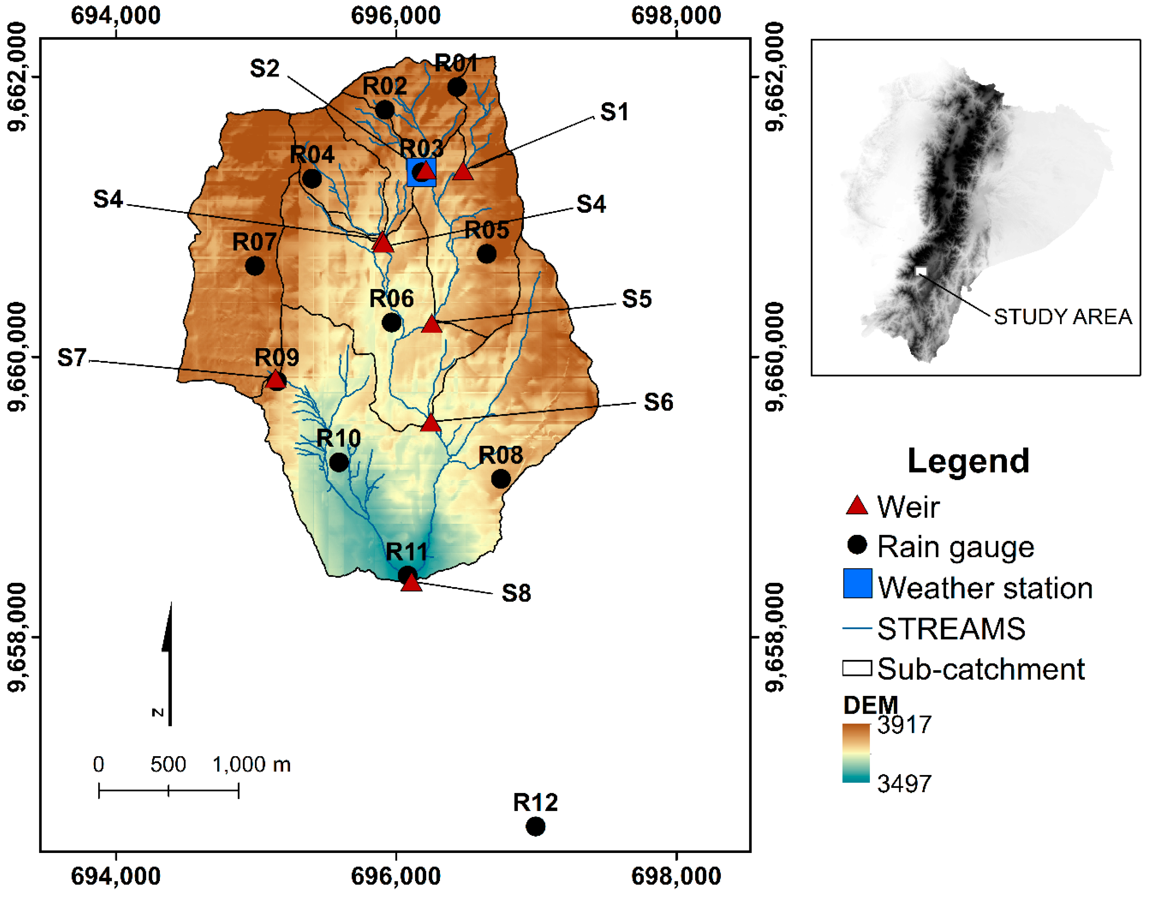
This study was carried out in the Zhurucay Ecohydrological Observatory located in the southern Ecuadorian Andes, near the continental divide, draining into the Pacific Ocean. The observatory consists of a nested catchment of 7.53 km2 with elevation ranging from 3400 to 3900 m a.s.l. (Figure 1). Mean annual precipitation is 1345 mm at 3780 m a.s.l. with weak seasonality. Rain mainly falls as drizzle and occurs almost daily [17]. Mean annual temperature is 6.0 °C [14]. The geomorphology of the catchment is glacial U-shaped. The average slope is 10°, although slopes up to 73° are found. The geology is compacted volcanic rock deposits formed during the last ice age [60]. In the northeastern of the catchment there is a ponded wetland at a flat hilltop. This structure drains towards the outlet of subcatchment S7 and occupies almost the entire subcatchment [21].
The main soil type in Zhurucay are Andosols (Ah horizon), covering 80% of the area and commonly located on the hillslopes. Histosols (H horizon) cover the 20% remaining area and are commonly located in flat areas where geomorphology allows water accumulation. These soils, formed in wetlands, are highly organic and are saturated most of the year [19]. Both soil types were formed by volcanic ash accumulation; they are black, humic, acid, and rich in organic carbon and are located over a mineral horizon (C horizon) commonly rich in clay [21,61].
The vegetation within the catchment is highly correlated with soil type [19] and is typical of páramo grasslands. Tussock grasses grow in Andosols while cushion plants grow in Histosols wetlands [4,62], covering 70% and 25% of the area, respectively. The remaining 5% of the area is covered by polylepis trees and pine forest. Since the percentage of polylepis and pine forest is too low within each subcatchment, these vegetation covers were not included in the study. Further description of landscape characteristics are provided in Mosquera et al. [19].
2.2. Monitoring and Data Availability
The Zhurucay Ecohydrological Observatory was established in 2009 with the purpose of studying the hydrological functioning of Andean mountain catchments. Over the years, it has been equipped with two automatic meteorological stations, a laser disdrometer, five permanent rain gauges, a nested hydrological network consisting of 10 weirs, a hillslope to study subsurface processes, and an environmental water quality monitoring system to study runoff flowpaths and runoff formation using isotopes and metals (in soils, streams, rainfall, and springs). Recent additions include an energy balance and eddy covariance system, and small-scale lysimeters.
At the beginning of 2013, the hydrological network was fully operational. For this experiment, the rain gauge network (five permanent rain gauges) was complemented with a total of 12 rain gauges: 11 were located inside the catchment and one was located 2 km downstream of the outlet. During the experiment, this rain gauge network was arguably the densest network in the Andes mountains at this spatial scale (1.46 rain gauges per km2). The extended network operated from 2014 to 2016. Hence, daily data of precipitation, temperature, potential evapotranspiration, and runoff corresponding to the period October 2013 to October 2016 were selected for this study. These variables were used according to the requirements of the HBV-light model. Precipitation data for the first study year was obtained from the five permanent rain gauges, and for the remaining years from the 12 rain gauges. Temperature and meteorological variables to estimate potential evapotranspiration were acquired from a weather station at 3780 m a.s.l. Runoff data were obtained from V-notch weirs at the outlets of seven subcatchments (S1 to S7) and from one rectangular weir at the outlet of Zhurucay catchment (S8) which is the focus of this study. Figure 1 shows the distribution of sensors and subcatchments. Subcatchments aggregated area and vegetation cover are presented in Table 1 which was provided by Mosquera et al. [19].
3. Methodology
First, we calibrated and validated each model structure using all rain gauges located inside the catchment. Each model structure was evaluated and compared according to the ability to simulate total runoff and its subflow components in order to select the model structure with the highest performance. Then, the model structure selected previously was calibrated and validated using six rainfall monitoring scenarios to evaluate the impact of rainfall estimation on the simulated runoff and parameters. Finally, the calibrated parameters with the worst rainfall scenario were employed to run the model with the remaining scenarios to analyze the possibility to enhance runoff simulation by improving rainfall information. The methodological details are explained in the following subsections.
3.1. HBV-Light Model
The HBV-light model [63] is a semidistributed conceptual rainfall-runoff model based on the original HBV model developed by Bergström [64] and Bergström [57] at the Swedish Meteorological and Hydrological Institute (SMHI). This model can be distributed into different elevation and vegetation zones as well as subcatchments. HBV-light uses four routines to simulate runoff: (i) the snow routine represents snow accumulation and snow melt; (ii) the soil routine describes ground water recharge and actual evaporation as function of water storage for each elevation or vegetation zone; (iii) the response routine computes the runoff as function of water stored in reservoirs; and (iv) the routing routine simulates the routing of the runoff to the outlet of the catchment by a triangular weighting function. Before the routing routine, runoff from previous subcatchments are added to the generated runoff of the current subcatchment. A detailed description of the model can be found in Seibert and Vis [65].
The standard model consists of two serial reservoirs that receive water from the semidistributed soil routine. Storage in the upper soil reservoir (SUZ) simulates fast flow and interflow, representing the near surface and subsurface flow, respectively; while storage in the lower soil reservoir (SLZ) simulates slow flow, representing baseflow. Both reservoirs are connected by a percolation rate. In total, HBV-light offers 11 different structures of reservoirs varying from one to three reservoirs with varying degrees of spatial distribution according to elevation and vegetation zones. Further details of model structures are found in Uhlenbrook et al. [66].
For this study, the Zhurucay catchment was divided into eight subcatchments and two vegetation zones representing tussock grasses (grassland) and cushion plants (wetlands). Runoff for each subcatchment were simulated considering the contribution of previous subcatchments, and therefore, the runoff simulation of subcatchment S8 is the simulation of the whole Zhurucay catchment. Structures related to snow and very slow flow were not used since Zhurucay does not receive snow. Eight model structures were used in this study, as presented in Table 2.
3.2. Model Calibration and Validation
The HBV-light model was calibrated using the standard split sample model calibration procedure [67,68]. The first, second, and third year of data (October 2013–October 2016) were used for model warming up, calibration, and validation, respectively. A year of data for each calibration and validation period were considered sufficient because of they cover the hydrological cycle of the study catchment. For the warming up period, spatial rainfall was estimated from the five permanent rain gauges (R03, R06, R07, R08, and R12), by inverse distance weighting (IDW) interpolation. This interpolation method was used due to the reduced number of rain gauges available. For the calibration and validation periods (years two and three) rainfall was estimated from the 11 rain gauges located inside the catchment, interpolated by ordinary Kriging. Potential evapotranspiration was estimated by the Penman–Monteith method [69] which has been used previously in Zhurucay [14].
The Monte Carlo procedure established by the HBV-light model was used to select an optimal parameter set after performing 10,000 simulations. Table 3 lists all parameters used and their calibration range. Parameter sets were generated using random numbers from a uniform distribution. The recession coefficient for fast flow (K0) was not calibrated and was set to 0.99 day−1 (close to one day). Interflow (K1) and slow flow (K2) coefficients were calibrated between relative fast ranges. These considerations were taken due to the fast recession observed in these subcatchments. The simulation results for each set of parameters in the Monte Carlo procedure were optimized by selecting the Nash-Sutcliffe efficiency (NSeff) [70] as the objective function.
3.3. Evaluation of Model Structures
Model structures were evaluated in two steps. First, for each model structure, HBV-light was calibrated and validated based on NSeff. Nevertheless, other performance indexes such as Nash-Sutcliffe efficiency with logarithms (Log NSeff), coefficient of determination (R2) and percentage annual difference (%ADiff) were additionally calculated to provide more information about the quality of the simulation [71,72]. NSeff has been widely used to evaluate the performance of hydrological models and it is sensitive to differences in the observed and simulated means and variances. Log NSeff is the NSeff using the logarithm of the runoff values reducing its sensitivity of extreme values. R2 describes how much of the observed dispersion is explained by the prediction. %ADiff is the percentage difference of the total observed runoff against the total simulated runoff used to observe the under or overestimation in the water balance.
Second, to identify the most behavioral models, the simulated runoff generated from the different storages of the model structures (e.g., STZ, SUZ, and SLZ) representing fast flow (FF), interflow (IF), and slow flow (SF) were compared to the flow components derived from measured runoff using the Water Engineering Time Series PROcessing tool (WETSPRO) [73]. WETSPRO is a tool that extracts the subflow components of a hydrograph based on Chapman filter [74] and using its recession constants (K) and the average fraction of each subflow component over the total flow (w). This tool has been used successfully to separate flow components and to test models by multicriteria approach [75,76,77]. Since model structures M1 and M3 simulate only two flow components, e.g., slow flow and the combination of interflow and fast flow, WETSPRO-derived interflow and fast flow were added for an adequate comparison.
3.4. Rainfall Monitoring Scenarios
We selected six rainfall-monitoring scenarios. These scenarios ranged from using all the rainfall network to using a single rain gauge located outside the catchment; they are described in Table 4. The first scenario (referred to as E0) uses 11 rain gauges inside the catchment and therefore provides the best rainfall estimation. The remaining five monitoring scenarios (E1–E5) were selected based on common practices used by water managers in the region. They simulate an scarce network by reducing the number of gauges as follows: one configuration using three rain gauges located in the upper, middle, and lower catchment (R01, R06, and R11) and four configurations using only one rain gauge in each one, located in the upper (R01), middle (R06), lower (R11), and outside the catchment (R12). For scenarios based on one rain gauge, spatial rainfall was considered uniform throughout the catchment. For the three-rain-gauge scenario, spatial rainfall was interpolated by inverse distance weighting (IDW). This method was selected rather than ordinary kriging due to the low rain gauge density.
3.5. Evaluation of the Quality of Spatial Rainfall Estimation
The best rainfall estimation (E0) was compared to the estimations obtained from the different monitoring scenarios (E1 to E5) as a way to understand the impact of the degraded rain gauge network. For this purpose, we used an analysis of scatter plot, R2 and the Goodness of Rainfall Estimation index (GORE) [50]. GORE was used to quantify the quality of the estimated rainfall time distribution. GORE is the transposition of NSeff in the precipitation domain, using the square root of the rainfall data to reduce the weight of extreme events and is expressed as:
where, n is the number of time steps of the period, is the estimated rainfall from rainfall monitoring scenario at time , is the best estimated rainfall available from rainfall monitoring scenario at time , and is the mean of the best estimated rainfall available (considered as reference) over the study period. Like NSeff, the GORE index varies between −∞ and 1, where 1 represents that the estimated rainfall is equal to the reference. GORE will be smaller as the rainfall estimates become poorer.
3.6. Evaluation of the Impact of Spatial Rainfall Estimation on Model Calibration
To evaluate the effect of the reduction of precipitation information by operating a sparse precipitation network on hydrological simulation, the HBV-light structure selected in Section 3.3 was calibrated and validated using each of the rainfall scenarios in Section 3.4. The performance of the simulated runoff (using NSeff) and calibrated parameters were related to the quality of the estimated rainfall (GORE) used to run the model.
Besides GORE index, BALANCE index was used to quantify the overestimation or underestimation of the total estimated rainfall and its relation to the model performance (NSeff) [50]. BALANCE index is greater than 1 in the case of rainfall overestimation and smaller than 1 in the case of underestimation, and is expressed as:
3.7. Effect of Improved Rainfall Estimation on A Model Calibrated with Scarce Data
For this objective, the model calibrated with the worst rainfall scenario was run using the input rainfall of the estimates from the remaining rainfall scenarios in a step-wise fashion, i.e., by improving the spatial rainfall estimation step-by-step up to the reference scenario (E0). Then, the performances of runoff simulations (NSeff index) were analyzed regarding the quality of rainfall information (GORE index) used to run the model.
4. Results and Discussion
4.1. Evaluation of the Model Structures
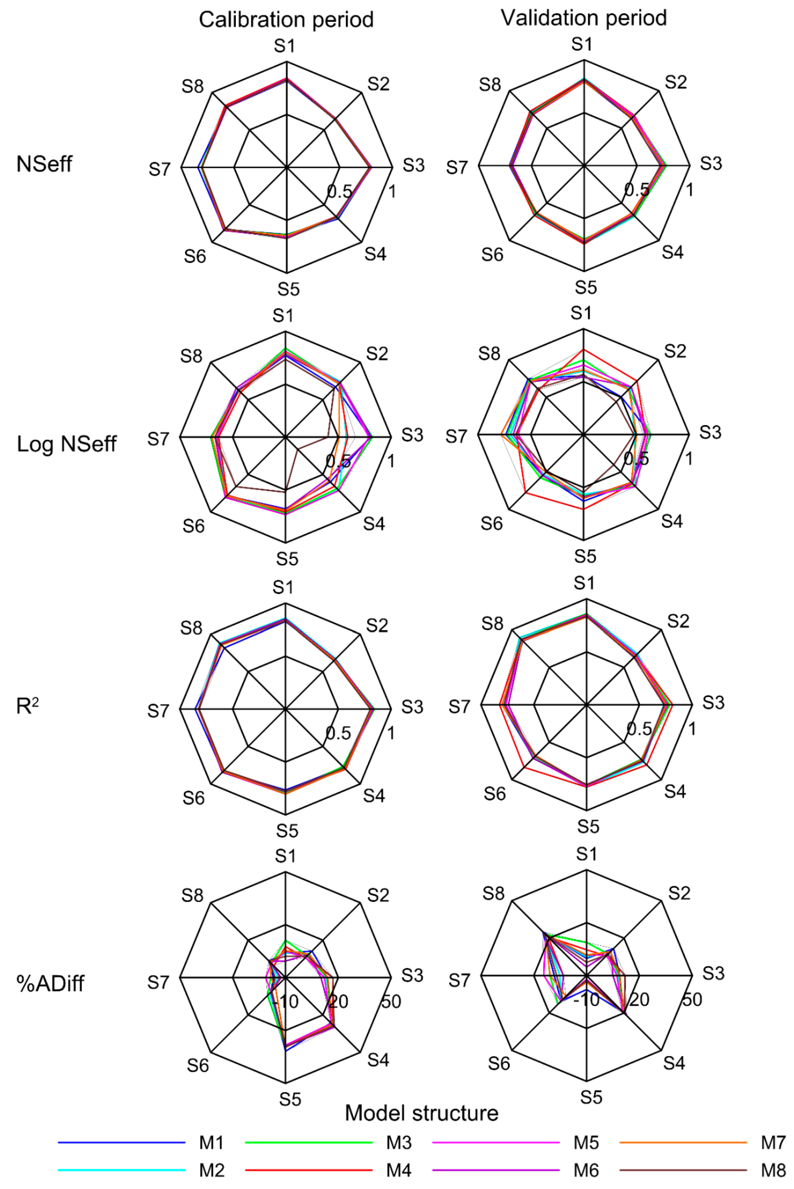
The performances of the eight model structures, for each subcatchment and for calibration and validation periods are shown in Figure 2. Each line represents a model structure and the overlapping of these lines indicates that all model structures have very similar performances. Indexes values can be found in supplementary Tables S1 and S2. From the magnitudes of NSeff, LogNSeff, R2, and %ADiff, it is hard to identify a model structure that outperforms the others, as there is little difference among them. Similar results were found by Uhlenbrook et al. [66] using six structures of HBV model in a mountainous catchment in Germany where NSeff values varied between 0.825 and 0.876 in the calibration period. This suggests that model parameters compensate for the differences among structures. Additionally, similar results are observed for all subcatchments, which can be explained by two reasons. First, the reason explained previously and second, that physical differences between subcatchments are not large enough to produce an impact in specific model structures [78].
For the catchment S8, which is the outlet of Zhurucay and the focus of this study, the NSeff values from eight structures vary between 0.80 and 0.83 and 0.68 and 0.73 for calibration and validation, respectively. These results were similar than those obtained by Buytaert and Beven [30] in a páramo catchment of 2.53 km2 with similar vegetation cover and altitude. The study evaluated nine model structures with NSeff values between 0.72 and 0.87 and 0.45 and 0.77 for calibration and validation, respectively; showing that HBV-light structures reached expected efficiencies for this ecosystem.
Considering these high NSeff values and the high R2 values (over 0.82), one might consider that the eight structures can represent the overall runoff dynamics. However, lower values of LogNSeff compared to NSeff suggest that structures may have problems to simulate low flows [71]. Therefore, we compared the observed and simulated subflow components for each model structure. This was done for the S8 catchment and the average of S1–S8 (Table 5).
The average of NSeff for all subcatchments shows low values for slow flow (SF) and fast flow (FF), below 0.37 and 0.20, respectively. For most of the structures, NSeff values showed high variability between subcatchments; for example, for the structure M2, slow flow NSeff ranges from 0.52 to −0.01. This shows that while model parameters can compensate the overall performance of a given model structure, the simulated subflow components do not represent the physical functioning of the catchments, and therefore these models are not behavioral [79].
For catchment S8, NSeff values for the eight model structures present similar results between subflow components, ranging from 0.17 to 0.42, 0.48 to 0.70, and 0.65 to 0.72 for SF, IF, and FF, respectively. These results indicate that SF was difficult to simulate; indeed, all model structures had NSeff values below 0.42 for this subflow. M1 was the model structure that obtained the highest performances (0.42 SF and 0.70 IF). Therefore, the M1 structure with two reservoirs that simulate slow flow and the combination of interflow and fast flow was chosen for the remaining of the study. The fact that the simplest structure showed the best performance in simulating all subflows suggests that the páramo ecosystem is hydrologically relatively simple [19], and that its water storage–release processes are mainly controlled by water moving laterally through the organic soils to the streams [22]. Thus, a two-reservoir model structure provided an accurate simulation of the observed runoff of the catchment.
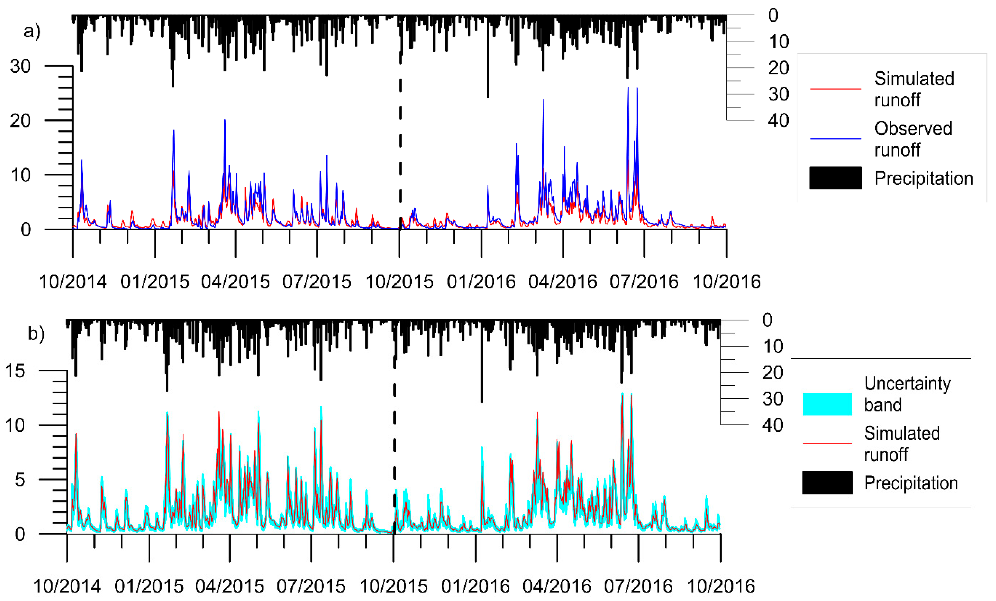
The best simulation according to NSeff (0.8 and 0.72 for calibration and validation, respectively) using the M1 structure for the subcatchment S8 (Zhurucay catchment) is shown in Figure 3. In addition, the optimal parameters found for this simulation are listed in Table 6. Temporarily we can observe that in general the simulation fits well to the dry and humid periods. However, there is a slight subestimation of the simulation in the peaks.
4.2. Evaluation of the Estimated Rainfall from Rainfall Monitoring Scenarios
The comparison of the daily rainfall estimated from the five monitoring scenarios (E1–E5) against the best rainfall estimation for the catchment (E0) is shown in Figure 4. It is observed that the scenario E1 using three rain gauges distributed in the upper, middle, and lower catchment represents well the spatial rainfall. For scenarios that use only one rain gauge to represent the spatial rainfall, scenario E3 (placing the rain gauge in the middle of the catchment) gives the best estimation. This result is similar to results observed by Hrachowitz and Weiler [80], and suggests that the rainfall observation in the middle of the catchment is very similar to the average of the rainfall of the entire catchments. On the other hand, it is observed that a rain gauge located in the upper catchment (E3) has better results than a rain gauge located in the lower catchment (E4). The quality of the estimation is reduced significantly when using rainfall observations from the rain gauge at 2 km downstream of the outlet (E5), producing a large scatter and overestimation. These results indicate that in this mountain setting there is a large rainfall variability at short distances, in line with results found by Buytaert et al. [33] who indicated that páramo rainfall can be highly variable, even at short distances of 4 km, suggesting a strong orographic influence in rainfall.
4.3. Evaluation of the Impact of Rainfall Estimation on Hydrological Simulation
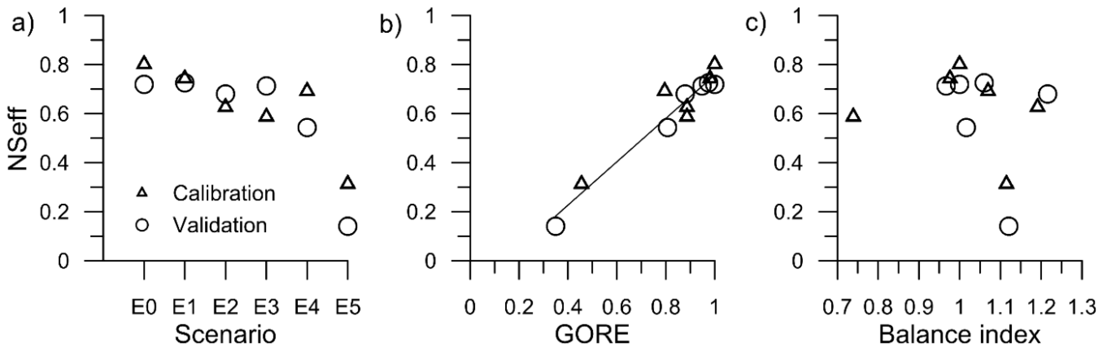
The impact of the rainfall estimation from the six monitoring scenarios on the performance of the simulated runoff is presented in Figure 5. This figure shows the model performance (NSeff) against the rainfall scenario (Figure 5a), the quality of the estimated rainfall (GORE, Figure 5b), and the over- or underestimation of rainfall (Balance index, Figure 5c).
As can be seen in Figure 5a, rainfall scenarios E0 and E1 produce very similar, good results, for both calibration and validation periods. This corroborates that the good rainfall quality of scenario E1 identified in Section 4.2, is also translated into a good runoff simulation. On the other hand, and as expected, the rainfall scenario with the worst rainfall quality (E5) produces the poorest runoff simulation (below 0.31 NSeff). Similar to results of Zhang and Han [81], we can observe in the rainfall scenario E5 that the model performance decreased drastically when the spatial rainfall variability is not considered. Model performance using rainfall scenarios with one rain gauge deteriorates when compared to the best spatial rainfall. And, although the validation period seems satisfactory for scenarios E2 and E3, the efficiency in the calibration period is significantly reduced. These results show how inadequate rainfall monitoring can produce high modeling uncertainty [36].
Additionally, we can observe in Figure 4 that E3 scenario shows better correlation than E4 with E0, however, in Figure 5, the E4 scenario gives better model performance for the calibration period compared with E3. The reason of the variation of the performance between calibration and validation periods can be due to annual variations that can be strongly affected by specific orographic factors.
Results also suggest that there is a direct relation between the rainfall quality (GORE) and the simulated runoff performance (NSeff), as can be seen in Figure 5b. Additionally, the slope of this relation is 0.88 indicating that a slight reduction in the quality of the estimated rainfall can produce a big reduction in the performance of the runoff simulation. This relation was also found in some Mediterranean catchments in France [49,50]. Nevertheless, the slope found in this study is more pronounced compared to the results of Andréassian et al. [50], which suggests a stronger influence of the quality of rainfall input on the runoff simulation in this mountain catchment.
Finally, the highest performance of the simulated runoff was obtained when the over- or underestimation of rainfall was minimal. According to the results of Andréassian et al. [50], it was expected that the performance of runoff simulation would increase when the Balance Index is closer to 1. This was found true when the Balance Index ranged from 1.07 to 0.97 (Figure 5c). However, above this range we found uncorrelated values of NSeff and BI (i.e., while for a BI of 1.11 we found a very low NSeff of 0.31, for a higher BI of 1.19 we found a NSeff of 0.63).
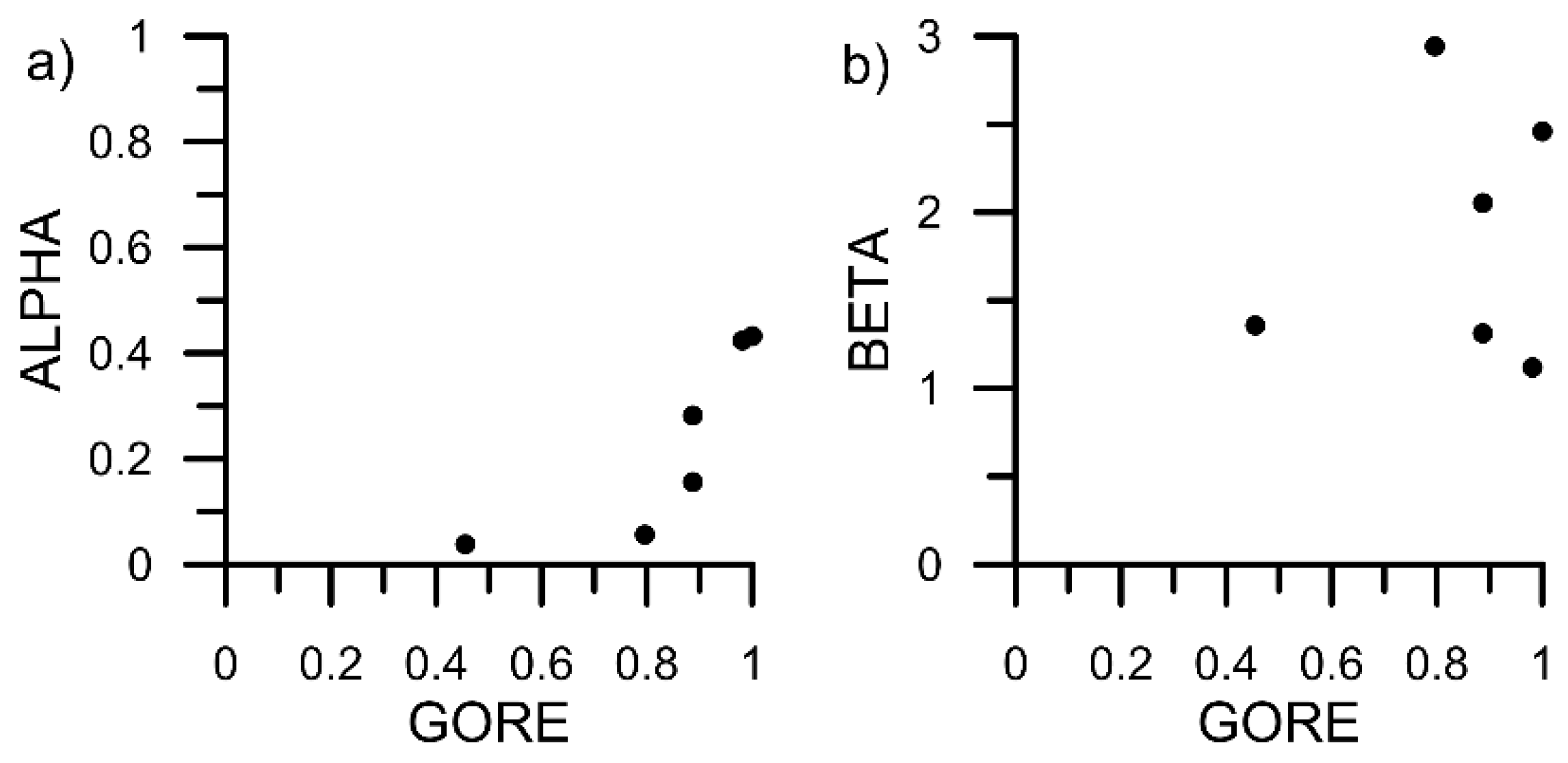
The sensibility of model parameters to rainfall quality is shown in Figure 6. ALPHA and BETA parameters are plotted against the GORE index. These two parameters were selected to illustrate their sensibility to rainfall quality.
The only parameter sensible to rainfall quality was ALPHA (Figure 6a). In the study of Andréassian et al. [50], the sensibility is expressed as the reduction of the variability of the parameter values as the rainfall quality increases until reaching an optimal parameter value. Our study indicated that the higher the GORE, the higher the ALPHA. On the other hand, Figure 6b shows BETA as example of a parameter showing no sensibility to rainfall quality. In contrast to the findings of Andréassian et al. [50], we found that the majority of parameters were not sensible to rainfall quality. This may be caused by the relative high number of parameters which allows an overadjustment to the input data compared to the three and six parameters used in Andréassian et al. [50]. Although, it is still an open question if the sensibility of parameters to the rainfall quality is a function of the number of parameters used by the model. Nevertheless, at least one parameter was found sensible, showing that despite this situation, rainfall quality may still have impact on the parameterization. This can be due to a correct estimation of precipitation which allows a better description of ALPHA parameter (which controls the amount of water that recharges the streams) to be adapted to the high water recharge of these soils.
4.4. Effect of Improved Rainfall Estimation in A Calibrated Model
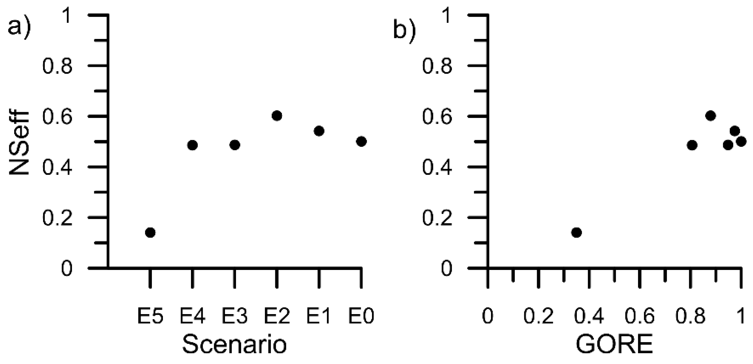
In this section, we analyzed the performance of the runoff simulation obtained from a calibrated model with far-from-perfect rainfall using new improved rainfall estimations. In this way, the model calibrated with input rainfall from scenario E5 was run for the validation period with the remaining scenarios. Figure 7 shows the NSeff index against the rainfall monitoring scenario and the GORE index.
Rainfall scenarios E4 to E0 produce a considerably better runoff simulation compared to scenario E5 (Figure 7a). Furthermore, NSeff values obtained from these scenarios were very similar and increased to 0.49–0.60 from an original value of 0.14. Additionally, in Figure 7b it is observed that high values of GORE are related to high values of NSeff, although, it was not found a direct relation between these two indexes.
In this way, better rainfall estimations produced an improvement in model performance. Similar results were found by Bárdossy and Das [42], who used 10 and 20 rain gauges for calibration and validation, respectively. Nevertheless, the improvement in the model efficiency was higher in our case. In this way, any improvement in rainfall monitoring will produce a big gain in modeling efficiency, even when using a model calibrated with far-from-perfect rainfall. Additionally, the fact that bad and good efficiencies can be obtained for the same parameters suggests that for this mountain ecosystem the rainfall input could be the biggest source of model uncertainty.
5. Conclusions
The present study was designed to assess the impact of rainfall estimation on hydrological modeling using six rainfall monitoring scenarios in a small headwater páramo catchment. This was achieved by installing a dense network of 12 rain gauges in the Zhurucay Ecohydrological Observatory in southern Ecuador, and creating rainfall scenarios by withdrawing a given number of rain gauges.
This study showed that all model structures of HBV-light model can represent total runoff. However, the capacity to simulate subflow components strongly varied between structures. The simplest model structure M1 (standard model) had the highest performance to represent subflow components, although all model structures have problems properly representing slow flow.
The research has also shown that having good spatial rainfall measurements is essential to achieve good modeling results in mountainous areas. We can conclude that a limited number of rain gauges can produce acceptable modeling performance. However, it strongly depends on the location of the rain gauges. In this case, three rain gauges in the upper, middle, and lower catchment worked well, but this has to be confirmed in other páramo catchments in order to generalize this knowledge. Furthermore, a better description of the spatial rainfall of the catchment not only enhances the runoff simulation but also the possibility to select an optimal parameter value.
Another significant finding that emerges from this study is that a calibrated model based on far-from-perfect rainfall estimates can produce acceptable runoff simulations when was run with new improved rainfall data, something that can be highly valuable by water managers.
Despite that rain gauges are considered the most trusted source of rainfall information, they are subject to errors. However, differences between rain gauges found here were larger (GORE from 0.41 to 0.98) than those caused by measurement errors. The effect of factors such as wind, elevation, topographic location, and mechanical errors on rainfall measuring were out of the scope of this study. Nevertheless, authors encourage the study of such factors mainly due to the lack of information about rainfall measuring on páramo ecosystem.
Overall, this study has showed that rainfall input could be the largest source of model uncertainty for this mountain ecosystem. Therefore, our findings have provided a first insight of the importance of rainfall monitoring for hydrological modeling in páramo catchments, which are the main water supply for millions of people.
Supplementary Materials
Supplementary materials can be found at https://www.mdpi.com/2073-4441/10/9/1169/s1. Table S1: Performance indexes (NSeff, Log NSeff, R2 and %ADiff) for calibration period. For eight sub-catchments (S1–S8) and eight model structures (M1–M8), Table S2: Performance indexes (NSeff, Log NSeff, R2 and %ADiff) for validation period. For eight sub-catchments (S1–S8) and eight model structures (M1–M8).
Author Contributions
A.S. analyzed the data and wrote the manuscript. R.C. designed and supervised the study and provided a critical revision of the manuscript.
Funding
This research was part of the project ‘‘Identificación de los procesos hidrometereológicos que desencadenan crecidas extremas en la ciudad de Cuenca” funded by the Dirección de Investigación of Universidad de Cuenca (DIUC) and the Empresa Pública Municipal de Telecomunicaciones, Agua Potable, Alcantarillado y Saneamiento de Cuenca (ETAPA-EP).
Acknowledgments
This manuscript is an outcome of UCuenca’s Master in Ecohydrology. The authors thank Johanna Orellana and Daniela Ballari for their collaboration in the development of the project. We are grateful to the staff and students that contributed to the hydrometeorological monitoring. We also thank Zhurucay’s Chumblin community that allowed the installation of equipment on its lands.
Conflicts of Interest
The authors declare no conflicts of interest. The founding sponsors had no role in the design of the study; in the collection, analyses, or interpretation of data; in the writing of the manuscript, and in the decision to publish the results.
References
- Hofstede, R.; Mena, V.; Segarra, P. Los Paramos del Mundo; Global Peatland Initiative/NC-IUCN/EcoCiencia: Quito, Ecuador, 2003. [Google Scholar]
- Josse, C.; Cuesta, F.; Navarro, G.; Barrena, V.; Cabrera, E.; Chacón-Moreno, E.; Ferreira, W.; Peralvo, M.; Saito, J.; Tovar, A. Atlas de los Andes del Norte y Centro. Bolivia, Colombia, Ecuador, Perú y Venezuela; Secretaría General de la Comunidad Andina, Programa Regional ECOBONA, CONDESAN-Proyecto Páramo Andino, Programa BioAndes, EcoCiencia, NatureServe, LTA-UNALM, IAvH, ICAE-ULA, CDC-UNALM, RUMBOL SRL: Lima, Perú, 2009. [Google Scholar]
- Pinos, J.; Studholme, A.; Carabajo, A.; Gracia, C. Leaf litterfall and decomposition of polylepis reticulata in the treeline of the Ecuadorian Andes. Mt. Res. Dev. 2016, 37, 87–96. [Google Scholar] [CrossRef]
- Sklenář, P.; Jørgensen, P.M. Distribution patterns of paramo plants in Ecuador. J. Biogeogr. 1999, 26, 681–691. [Google Scholar] [CrossRef]
- Sarmiento, L.; Llambí, L.D.; Escalona, A.; Marquez, N. Vegetation patterns, regeneration rates and divergence in an old-field succession of the high tropical Andes. Plant Ecol. 2003, 166, 145–156. [Google Scholar] [CrossRef] [Green Version]
- Viviroli, D.; Du, H.H.; Messerli, B.; Meybeck, M.; Weingartner, R. Mountains of the world, water towers for humanity: Typology, mapping, and global significance. Water Resour. Res. 2007, 43, W07447. [Google Scholar] [CrossRef]
- Buytaert, W.; De Bièvre, B. Water for cities: The impact of climate change and demographic growth in the tropical Andes. Water Resour. Res. 2012, 48, W08503. [Google Scholar] [CrossRef]
- Sarmiento, L. Water balance and soil loss under long fallow agriculture in the Venezuelan Andes. Mt. Res. Dev. 2000, 20, 246–253. [Google Scholar] [CrossRef]
- De Bièvre, B.; Alvarado, A.; Timbe, L.; Célleri, R.; Feyen, J. Night irrigation reduction for water saving in medium-sized systems. J. Irrig. Drain. Eng. 2003, 129, 108–116. [Google Scholar] [CrossRef]
- Buytaert, W.; Wyseure, G.; De Bièvre, B.; Deckers, J. The effect of land-use changes on the hydrological behaviour of Histic Andosols in south Ecuador. Hydrol. Process. 2005, 19, 3985–3997. [Google Scholar] [CrossRef] [Green Version]
- Crespo, P.; Célleri, R.; Buytaert, W.; Feyen, J.; Iñiguez, V.; Borja, P.; De Bièvre, B. Land use change impacts on the hydrology of wet Andean páramo ecocystems. In Status and Perspectives of Hydrology in Small Basins; IAHS Publ. 336; International Association for Hydrological Sciences: London, UK, 2009; pp. 71–76. [Google Scholar]
- Célleri, R.; Feyen, J. The hydrology of tropical Andean ecosystems: Importance, knowledge status, and perspectives. Mt. Res. Dev. 2009, 29, 350–355. [Google Scholar] [CrossRef] [Green Version]
- Carrillo-Rojas, G.; Silva, B.; Córdova, M.; Célleri, R.; Bendix, J. Dynamic mapping of evapotranspiration using an energy balance-based model over an Andean páramo catchment of southern Ecuador. Remote Sens. 2016, 8, 160. [Google Scholar] [CrossRef]
- Córdova, M.; Carrillo-Rojas, G.; Crespo, P.; Wilcox, B.; Célleri, R. Evaluation of the Penman-Monteith (FAO 56 PM) method for calculating reference evapotranspiration using limited data. Application to the wet páramo of southern Ecuador. Mt. Res. Dev. 2015, 35, 230–239. [Google Scholar] [CrossRef]
- Ochoa-Sánchez, A.; Crespo, P.; Célleri, R. Quantification of rainfall interception in the high Andean tussock grasslands. Ecohydrology 2018, 11. [Google Scholar] [CrossRef]
- Campozano, L.; Célleri, R.; Trachte, K.; Bendix, J.; Samaniego, E. Rainfall and cloud dynamics in the Andes: A southern Ecuador case study. Adv. Meteorol. 2016. [Google Scholar] [CrossRef]
- Padrón, R.S.; Wilcox, B.P.; Crespo, P.; Célleri, R. Rainfall in the Andean páramo: New insights from high-resolution monitoring in southern Ecuador. J. Hydrometeorol. 2015, 16, 985–996. [Google Scholar] [CrossRef]
- Crespo, P.; Feyen, J.; Buytaert, W.; Bücker, A.; Breuer, L.; Frede, H.G.; Ramírez, M. Identifying controls of the rainfall-runoff response of small catchments in the tropical Andes (Ecuador). J. Hydrol. 2011, 407, 164–174. [Google Scholar] [CrossRef]
- Mosquera, G.M.; Lazo, P.X.; Célleri, R.; Wilcox, B.P.; Crespo, P. Runoff from tropical alpine grasslands increases with areal extent of wetlands. Catena 2015, 125, 120–128. [Google Scholar] [CrossRef] [Green Version]
- Correa, A.; Windhorst, D.; Crespo, P.; Célleri, R.; Feyen, J.; Breuer, L. Continuous versus event based sampling: How many samples are required for deriving general hydrological understanding on Ecuador’s páramo region? Hydrol. Process. 2016, 30, 4059–4073. [Google Scholar] [CrossRef]
- Mosquera, G.M.; Segura, C.; Vaché, K.B.; Windhorst, D.; Breuer, L.; Crespo, P. Insights on the water mean transit time in a high-elevation tropical ecosystem. Hydrol. Earth Syst. Sci. 2016, 20, 2987–3004. [Google Scholar] [CrossRef]
- Mosquera, G.M.; Célleri, R.; Lazo, P.X.; Vaché, K.B.; Perakis, S.S.; Crespo, P. Combined use of isotopic and hydrometric data to conceptualize ecohydrological processes in a high-elevation tropical ecosystem. Hydrol. Process. 2016, 30, 2930–2947. [Google Scholar] [CrossRef] [Green Version]
- Ochoa-Tocachi, B.F.; Buytaert, W.; De Bièvre, B.; Célleri, R.; Crespo, P.; Villacís, M.; Llerena, C.A.; Acosta, L.; Villazón, M.; Guallpa, M.; et al. Impacts of land use on the hydrological response of tropical Andean catchments. Hydrol. Process. 2016, 30, 4074–4089. [Google Scholar] [CrossRef] [Green Version]
- Avilés, A.; Célleri, R.; Paredes, J.; Solera, A. Evaluation of Markov chain based drought forecasts in an Andean regulated river basin using the skill scores RPS and GMSS. Water Resour. Manag. 2015, 29, 1949–1963. [Google Scholar] [CrossRef]
- Avilés, A.; Célleri, R.; Solera, A.; Paredes, J. Probabilistic forecasting of drought events using Markov chain- and Bayesian network-based models: A case study of an Andean regulated river basin. Water 2016, 8, 37. [Google Scholar] [CrossRef]
- Flores-López, F.; Galaitsi, S.E.; Escobar, M.; Purkey, D. Modeling of Andean páramo ecosystems’ hydrological response to environmental change. Water 2016, 8, 94. [Google Scholar] [CrossRef]
- Buytaert, W.; De Bièvre, B.; Wyseure, G.; Deckers, J. The use of the linear reservoir concept to quantify the impact of changes in land use on the hydrology of catchments in the Andes. Hydrol. Earth Syst. Sci. 2004, 8, 108–114. [Google Scholar] [CrossRef] [Green Version]
- Buytaert, W.; Iñiguez, V.; Célleri, R.; Wyseure, G.; Deckers, J. Analysis of the water balance of small páramo catchments in south Ecuador. In Environmental Role of Wetlands in Headwaters; Krecek, J., Haigh, M., Eds.; Springer: Dordrecht, The Netherlands, 2006; pp. 271–281. [Google Scholar]
- Espinosa, J.; Rivera, D. Variations in water resources availability at the Ecuadorian páramo due to land-use changes. Environ. Earth Sci. 2016, 75, 1173. [Google Scholar] [CrossRef]
- Buytaert, W.; Beven, K. Models as multiple working hypotheses: hydrological simulation of tropical alpine wetlands. Hydrol. Process. 2011, 25, 1784–1799. [Google Scholar] [CrossRef]
- Crespo, P.; Feyen, J.; Buytaert, W.; Célleri, R.; Frede, H.-G.; Ramírez, M.; Breuer, L. Development of a conceptual model of the hydrologic response of tropical Andean micro-catchments in southern Ecuador. Hydrol. Earth Syst. Sci. Discuss. 2012, 9, 2475–2510. [Google Scholar] [CrossRef]
- Célleri, R.; Willems, P.; Buytaert, W.; Feyen, J. Space–time rainfall variability in the Paute basin, Ecuadorian Andes. Hydrol. Process. 2007, 21, 3316–3327. [Google Scholar] [CrossRef] [Green Version]
- Buytaert, W.; Célleri, R.; Willems, P.; De Bièvre, B.; Wyseure, G. Spatial and temporal rainfall variability in mountainous areas: A case study from the south Ecuadorian Andes. J. Hydrol. 2006, 329, 413–421. [Google Scholar] [CrossRef] [Green Version]
- Arnaud, P.; Bouvier, C.; Cisneros, L.; Dominguez, R. Influence of rainfall spatial variability on flood prediction. J. Hydrol. 2002, 260, 216–230. [Google Scholar] [CrossRef]
- Beven, K.; Homberger, G.M. Assessing the effect of spatial pattern of precipitation in modeling stream flow hydrographs. Water Resour. Bull. 1982, 18, 823–829. [Google Scholar] [CrossRef]
- Chang, C.-L.; Lo, S.-L.; Chen, M.-Y. Uncertainty in watershed response predictions induced by spatial variability of precipitation. Environ. Monit. Assess. 2007, 127, 147–153. [Google Scholar] [CrossRef] [PubMed]
- Chaubey, I.; Haan, C.T.; Salisbury, J.M.; Grunwald, S. Quantifying model output uncertainty due to spatial variability of rainfall. J. Am. Water Resour. Assoc. 1999, 35, 1113–1123. [Google Scholar] [CrossRef]
- Obled, C.; Wendling, J.; Beven, K. The sensitivity of hydrological models to spatial rainfall patterns: An evaluation using observed data. J. Hydrol. 1994, 159, 305–333. [Google Scholar] [CrossRef]
- Rouhier, L.; Le Lay, M.; Garavaglia, F.; Le Moine, N.; Hendrickx, F.; Monteil, C.; Ribstein, P. Impact of mesoscale spatial variability of climatic inputs and parameters on the hydrological response. J. Hydrol. 2017, 553, 13–25. [Google Scholar] [CrossRef]
- Younger, P.M.; Freer, J.E.; Beven, K. Detecting the effects of spatial variability of rainfall on hydrological modelling within an uncertainty analysis framework. Hydrol. Process. 2009, 23, 1988–2003. [Google Scholar] [CrossRef]
- Faurés, J.-M.; Goodrich, D.C.; Woolhiser, D.A.; Sorooshian, S. Impact of small-scale spatial rainfall variability on runoff modeling. J. Hydrol. 1995, 173, 309–326. [Google Scholar] [CrossRef]
- Bárdossy, A.; Das, T. Influence of rainfall observation network on model calibration and application. Hydrol. Earth Syst. Sci. 2008, 12, 77–89. [Google Scholar] [CrossRef] [Green Version]
- Xu, H.; Xu, C.-Y.; Chen, H.; Zhang, Z.; Li, L. Assessing the influence of rain gauge density and distribution on hydrological model performance in a humid region of China. J. Hydrol. 2013, 505, 1–12. [Google Scholar] [CrossRef]
- Berne, A.; Delrieu, G.; Creutin, J.-D.; Obled, C. Temporal and spatial resolution of rainfall measurements required for urban hydrology. J. Hydrol. 2004, 299, 166–179. [Google Scholar] [CrossRef]
- Pechlivanidis, I.G.; McIntyre, N.; Wheater, H.S. The significance of spatial variability of rainfall on runoff: An evaluation based on the Upper Lee catchment, UK. Hydrol. Res. 2016, 48, 478–485. [Google Scholar] [CrossRef]
- Syed, K.H.; Goodrich, D.C.; Myers, D.E.; Sorooshian, S. Spatial characteristics of thunderstorm rainfall fields and their relation to runoff. J. Hydrol. 2003, 271, 1–21. [Google Scholar] [CrossRef]
- Singh, V.P. Effect of spatial and temporal variability in rainfall and watershed characteristics on stream flow hydrograph. Hydrol. Process. 1997, 11, 1649–1669. [Google Scholar] [CrossRef]
- Lobligeois, F.; Andréassian, V.; Perrin, C.; Tabary, P.; Loumagne, C. When does higher spatial resolution rainfall information improve streamflow simulation? An evaluation using 3620 flood events. Hydrol. Earth Syst. Sci. 2014, 18, 575–594. [Google Scholar] [CrossRef] [Green Version]
- Anctil, F.; Lauzon, N.; Andréassian, V.; Oudin, L.; Perrin, C. Improvement of rainfall-runoff forecasts through mean areal rainfall optimization. J. Hydrol. 2006, 328, 717–725. [Google Scholar] [CrossRef]
- Andréassian, V.; Perrin, C.; Michel, C.; Usart-Sanchez, I.; Lavabre, J. Impact of imperfect rainfall knowledge on the efficiency and parameters of watershed models. J. Hydrol. 2004, 250, 206–235. [Google Scholar] [CrossRef]
- Segond, M.-L.; Wheater, H.S.; Onof, C. The significance of spatial rainfall representation for flood runoff estimation: A numerical evaluation based on the Lee catchment, UK. J. Hydrol. 2007, 347, 116–131. [Google Scholar] [CrossRef]
- Arnaud, P.; Lavabre, J.; Fouchier, C.; Diss, S.; Javelle, P. Sensitivity of hydrological models to uncertainty in rainfall input. Hydrol. Sci. J. 2011, 56, 397–410. [Google Scholar] [CrossRef] [Green Version]
- Girons Lopez, M.; Seibert, J. Influence of hydro-meteorological data spatial aggregation on streamflow modelling. J. Hydrol. 2016, 541, 1212–1220. [Google Scholar] [CrossRef]
- Célleri, R.; Buytaert, W.; De Bièvre, B.; Tobón, C.; Crespo, P.; Molina, J.; Feyen, J. Understanding the hydrology of tropical Andean ecosystems through an Andean Network of Basins. IAHS-AISH 2010, 336, 209–212. [Google Scholar] [CrossRef]
- Aparecido, L.M.T.; Teodoro, G.S.; Mosquera, G.; Brum, M.; Barros, F.d.V.; Pompeu, P.V.; Rodas, M.; Lazo, P.; Müller, C.S.; Mulligan, M.; et al. Ecohydrological drivers of Neotropical vegetation in montane ecosystems. Ecohydrology 2018, 11. [Google Scholar] [CrossRef]
- Wright, C.; Kagawa-Viviani, A.; Gerlein-Safdi, C.; Mosquera, G.M.; Poca, M.; Tseng, H.; Chun, K.P. Advancing ecohydrology in the changing tropics: Perspectives from early career scientists. Ecohydrology 2018, 11. [Google Scholar] [CrossRef]
- Bergström, S. The HBV Model: Its Structure and Applications; SMH1 Reports Hydrology No. 4; Swedish Meteorological and Bydrological Institute: Norrkoping, Sweden, 1992.
- Plesca, I.; Timbe, E.; Exbrayat, J.-F.; Windhorst, D.; Kraft, P.; Crespo, P.; Vaché, K.B.; Frede, H.-G.; Breuer, L. Model intercomparison to explore catchment functioning: Results from a remote montane tropical rainforest. Ecol. Model. 2012, 239, 3–13. [Google Scholar] [CrossRef] [Green Version]
- Steele-Dunne, S.; Lynch, P.; Mcgrath, R.; Semmler, T.; Wang, S.; Hanafin, J.; Nolan, P. The impacts of climate change on hydrology in Ireland. J. Hydrol. 2008, 356, 28–45. [Google Scholar] [CrossRef]
- Coltorti, M.; Ollier, C.D. Geomorphic and tectonic evolution of the Ecuadorian Andes. Geomorphology 2000, 32, 1–19. [Google Scholar] [CrossRef]
- Quichimbo, P.; Tenorio, G.; Borja, P.; Cárdenas, I.; Crespo, P.; Célleri, R. Efectos sobre las propiedades físicas y químicas de los suelos por el cambio de la cobertura vegetal y uso del suelo: Páramo de Quimsacocha al sur del Ecuador. Suelos Ecuatoriales 2012, 42, 138–153. [Google Scholar]
- Ramsay, P.M.; Oxley, E.R.B. The growth form composition of plant communities in the Ecuadorian paramos. Plant Ecol. 1997, 131, 173–192. [Google Scholar] [CrossRef]
- Seibert, J. Estimation of parameter uncertainty in the HBV model. Nord. Hydrol. 1997, 28, 247–262. [Google Scholar] [CrossRef]
- Bergström, S. Development and Application of a Conceptual Runoff Model for Scandinavian Catchments; SMHI Report RHO 7; Swedish Meteorological and Hydrological Institute: Norrköping, Sweden, 1976.
- Seibert, J.; Vis, M.J.P. Teaching hydrological modeling with a user-friendly catchment-runoff-model software package. Hydrol. Earth Syst. Sci. 2012, 16, 3315–3325. [Google Scholar] [CrossRef] [Green Version]
- Uhlenbrook, S.; Seibert, J.; Rodhe, A. Prediction uncertainty of conceptual rainfall-runoff models caused by problems in identifying model parameters and structure. Hydrol. Sci. J. 1999, 44, 779–797. [Google Scholar] [CrossRef] [Green Version]
- Ewen, J.; Parkin, G. Validation of catchment models for predicting land-use and climate change impacts. 1. Method. J. Hydrol. 1996, 175, 583–594. [Google Scholar] [CrossRef]
- Klemeš, V. Operational testing of hydrological simulation models. Hydrol. Sci. J. 1986, 31, 13–24. [Google Scholar] [CrossRef] [Green Version]
- Allen, R.G.; Pereira, L.; Raes, D.; Smith, M. Crop Evapotranspiration: Guidelines for Computing Crop Requirements; FAO Irrigation and Drainage Paper No. 56; Food and Agriculture Organization of the United Nations: Rome, Italy, 1998. [Google Scholar]
- Nash, J.E.; Sutcliffe, J.V. River flow forecasting through conceptual models part I—A discussion of principles. J. Hydrol. 1970, 10, 282–290. [Google Scholar] [CrossRef]
- Krause, P.; Boyle, D.P.; Bäse, F. Comparison of different efficiency criteria for hydrological model assessment. Adv. Geosci. 2005, 5, 89–97. [Google Scholar] [CrossRef]
- Legates, D.R.; McCabe, G.J., Jr. Evaluating the use of “goodness of fit” measures in hydrologic and hydroclimatic model validation. Water Resour. Res. 1999, 35, 233–241. [Google Scholar] [CrossRef]
- Willems, P. A time series tool to support the multi-criteria performance evaluation of rainfall-runoff models. Environ. Model. Softw. 2009, 24, 311–321. [Google Scholar] [CrossRef]
- Chapman, T.G. Comment on “Evaluation of automated techniques for base flow and recession analyses” by R. J. Nathan and T. A. McMahon. Water Resour. Res. 1991, 27, 1783–1784. [Google Scholar] [CrossRef] [Green Version]
- Shakti, P.C.; Shrestha, N.K.; Gurung, P. Step wise multi-criteria performance evaluation of rainfall-runoff models using WETSPRO. J. Hydrol. Meteorol. 2010, 7, 18–29. [Google Scholar] [CrossRef]
- Rubarenzya, M.H.; Willems, P.; Berlamont, J.; Feyen, J. Application of multi-criteria tool in MIKE SHE model development and testing. In Proceedings of the 2006 World Environmental and Water Resources Congress, Omaha, Nebraska, 21–25 May 2006. [Google Scholar] [CrossRef]
- Chawanda, C.J.; Nossent, J.; Bauwens, W. Baseflow Separation Tools; What do they really do? In Proceedings of the 19th EGU General Assembly, EGU2017, Vienna, Austria, 23–28 April 2017; Volume 19, p. 18768. [Google Scholar]
- Seibert, J. Regionalisation of parameters for a conceptual rainfall-runoff model. Agric. For. Meteorol. 1999, 98–99, 279–293. [Google Scholar] [CrossRef]
- Gupta, H.V.; Beven, K.; Wagener, T. Model calibration and uncertainty estimation. In Encyclopedia of Hydrological Sciences; John Wiley & Sons, Ltd.: Chichester, UK, 2006. [Google Scholar]
- Hrachowitz, M.; Weiler, M. Uncertainty of precipitation estimates caused by sparse gauging networks in a small, mountainous watershed. J. Hydrol. Eng. 2011, 16, 460–471. [Google Scholar] [CrossRef]
- Zhang, J.; Han, D. Assessment of rainfall spatial variability and its influence on runoff modelling: A case study in the Brue catchment, UK. Hydrol. Process. 2017, 31, 2972–2981. [Google Scholar] [CrossRef]
Figure 1.
Study area and monitoring network. Coordinate system: UTM WGS84 17S.

Figure 2.
Performance indexes for the simulated runoff. Left column for calibration period and right column for validation period. Each axis represents a subcatchment (S1–S8) and each colored line represents a model structure (M1–M8).
Figure 2.
Performance indexes for the simulated runoff. Left column for calibration period and right column for validation period. Each axis represents a subcatchment (S1–S8) and each colored line represents a model structure (M1–M8).

Figure 3.
(a) Best simulated (according to NSeff) runoff for the subcatchment S8 (Zhurucay catchment) using the M1 structure (with the optimal parameters) and the observed runoff. (b) Best simulated (according to NSeff) runoff for the subcatchment S8 (Zhurucay catchment) using the M1 structure (with the optimal parameters) and its uncertainty band corresponding to the 5–95% confidence limits of the possible solutions from the 10,000 Monte Carlo simulations. The dashed line indicates the end of the calibration period and the start of the validation period.

Figure 4.
Scatter plot, determination coefficient (R2), and GORE of the estimated spatial rainfall of catchment S8 from monitoring scenarios E1–E5 (axis X) against the reference estimated rainfall from monitoring scenario E0 (axis Y).
Figure 4.
Scatter plot, determination coefficient (R2), and GORE of the estimated spatial rainfall of catchment S8 from monitoring scenarios E1–E5 (axis X) against the reference estimated rainfall from monitoring scenario E0 (axis Y).

Figure 5.
Impact of rainfall quality on model performance (NSeff) against: (a) rainfall monitoring scenario, (b) GORE index, and (c) Balance Index. For calibration and validation period.
Figure 5.
Impact of rainfall quality on model performance (NSeff) against: (a) rainfall monitoring scenario, (b) GORE index, and (c) Balance Index. For calibration and validation period.

Figure 6.
Sensibility of model parameters to rainfall quality (GORE). (a) For a parameter sensible, ALPHA and (b) for a parameter no sensible, BETA.
Figure 6.
Sensibility of model parameters to rainfall quality (GORE). (a) For a parameter sensible, ALPHA and (b) for a parameter no sensible, BETA.

Figure 7.
Impact of rainfall quality on model performance (NSeff) of a calibrated model with low rainfall quality against (a) rainfall monitoring scenario and (b) GORE index.
Figure 7.
Impact of rainfall quality on model performance (NSeff) of a calibrated model with low rainfall quality against (a) rainfall monitoring scenario and (b) GORE index.


Table 1.
Subcatchment aggregated area and vegetation cover.
| Subcatchment | Aggregated Area (km2) | Vegetation Cover (%) | |
|---|---|---|---|
| Wetland | Tussock Grass | ||
| S1 | 0.20 | 15 | 85 |
| S2 | 0.38 | 13 | 87 |
| S3 | 0.38 | 18 | 82 |
| S4 | 0.65 | 18 | 82 |
| S5 | 1.40 | 17 | 83 |
| S6 | 3.28 | 24 | 76 |
| S7 | 1.22 | 65 | 35 |
| S8 | 7.53 | 25 | 75 |
Table 2.
HBV-light model structures.
| ID | Structure a |
|---|---|
| M1 | Two boxes (SUZ and SLZ, standard). |
| M2 | Two boxes (SUZ and SLZ). UZL threshold. |
| M3 | Two boxes (SUZ and SLZ). SUZ distributed. |
| M4 | Two boxes (SUZ and SLZ). SUZ distributed and UZL threshold. |
| M5 | Three boxes (STZ, SUZ and SLZ). |
| M6 | Three boxes (STZ, SUZ and SLZ). STZ distributed. |
| M7 | Three boxes (STZ, SUZ and SLZ). STZ and SUZ distributed. |
| M8 | One box. UZL and PERC thresholds. |
a STZ = Storage in top zone; SUZ = Storage in upper zone; SLZ = Storage in lower zone; UZL = Threshold parameter above which overland flow is produced; PERC = Threshold parameter above which interflow is produced.
Table 3.
HBV-light model parameters and their range used in the Monte Carlo procedure.
| Parameter | Description | Unit | Minimum | Maximum |
|---|---|---|---|---|
| Soil routinea | ||||
| FC | Maximum soil moisture | mm | 250 | 400 |
| LP | Soil moisture (MS) above which actual evapotranspiration reaches potential evapotranspiration (MS/FC) | - | 0.5 | 1 |
| BETA | Relative contribution to runoff from rain or snowmelt | - | 1 | 3 |
| Response routine | ||||
| K0 b | Recession coefficient for quick flow | day−1 | 0.999 | 0.999 |
| K1 | Recession coefficient for interflow | day−1 | 0.33 | 0.999 |
| K2 | Recession coefficient for baseflow | day−1 | 0.066 | 0.2 |
| ALPHA c | Nonlinearity coefficient | - | 0 | 1 |
| UZL d | Threshold parameter for K0 outflow | mm | 0 | 30 |
| PERC e | Percolation from SUZ to SLZ | mm day−1 | 0 | 2 |
| UZL f | Percolation from STZ to SUZ | mm day−1 | 0 | 30 |
| PERC g | Threshold parameter for K1 outflow | mm | 0 | 2 |
| Routing routine | ||||
| MAXBAS | Length of triangular weighting function | d | 1 | 1.5 |
a Parameters for each vegetation cover; b Parameter used only for structures M2, M4, M5, M6, M7, and M8; c Parameter used only for structures M1 and M3; d Parameter used only for structures M2, M4 and M8; e Parameter used only for structures M1, M2, M3, M4, M5, M6, and M7; f Parameter used only for structures M5, M6, and M7; g Parameter used only for structure M8; FC is the previous parameter and the expression defines the relationship to obtain LP.
Table 4.
Rainfall monitoring scenarios.
| ID | Rain Gauge(s) | Spatial Rainfall Estimation Method |
|---|---|---|
| E0 | R01 to R11 | Ordinary kriging |
| E1 | R01, R06, R11 | IDW |
| E2 | R01 | Punctual |
| E3 | R06 | Punctual |
| E4 | R11 | Punctual |
| E5 | R12 | Punctual |
Table 5.
Nash–Sutcliffe efficiency for simulated flow components from each model structure. For outlet subcatchment S8 and the average of S1–S8.
Table 5.
Nash–Sutcliffe efficiency for simulated flow components from each model structure. For outlet subcatchment S8 and the average of S1–S8.
| Model Structure | Flow Components S8 | Average Flow Component (S1–S8) | ||||
|---|---|---|---|---|---|---|
| SF | IF | FF | SF | IF | FF | |
| M1 | 0.42 | 0.70 | 0.32 | 0.72 | ||
| M2 | 0.17 | 0.68 | 0.67 | 0.07 | 0.61 | 0.08 |
| M3 | 0.33 | 0.67 | 0.37 | 0.71 | ||
| M4 | 0.28 | 0.64 | 0.72 | 0.13 | 0.60 | 0.27 |
| M5 | 0.39 | 0.48 | 0.66 | 0.27 | 0.52 | 0.16 |
| M6 | 0.35 | 0.53 | 0.65 | 0.05 | 0.55 | 0.20 |
| M7 | 0.36 | 0.62 | 0.66 | 0.19 | 0.55 | 0.09 |
| M8 | 0.31 | 0.63 | 0.70 | 0.05 | 0.60 | 0.30 |
Table 6.
Optimal parameters from the best runoff simulation according to NSeff.
| Routine | Parameter | Value |
|---|---|---|
| Soil routine 1 (Wetland) | FC_1 | 294.44 |
| LP_1 | 0.97 | |
| BETA_1 | 2.79 | |
| Soil routine 2 (Tussock grass) | FC_2 | 254.11 |
| LP_2 | 1.00 | |
| BETA_2 | 2.46 | |
| Response routine | PERC | 1.90 |
| ALPHA | 0.43 | |
| K1 | 0.42 | |
| K2 | 0.16 | |
| Routing routine | MAXBAS | 1.00 |
© 2018 by the authors. Licensee MDPI, Basel, Switzerland. This article is an open access article distributed under the terms and conditions of the Creative Commons Attribution (CC BY) license (http://creativecommons.org/licenses/by/4.0/).
Share and Cite
MDPI and ACS Style
Sucozhañay, A.; Célleri, R. Impact of Rain Gauges Distribution on the Runoff Simulation of a Small Mountain Catchment in Southern Ecuador. Water 2018, 10, 1169. https://doi.org/10.3390/w10091169
AMA Style
Sucozhañay A, Célleri R. Impact of Rain Gauges Distribution on the Runoff Simulation of a Small Mountain Catchment in Southern Ecuador. Water. 2018; 10(9):1169. https://doi.org/10.3390/w10091169
Chicago/Turabian StyleSucozhañay, Adrián, and Rolando Célleri. 2018. "Impact of Rain Gauges Distribution on the Runoff Simulation of a Small Mountain Catchment in Southern Ecuador" Water 10, no. 9: 1169. https://doi.org/10.3390/w10091169
Note that from the first issue of 2016, this journal uses article numbers instead of page numbers. See further details here.