Modified Richards’ Equation to Improve Estimates of Soil Moisture in Two-Layered Soils after Infiltration

Abstract

Soil moisture distribution plays a significant role in soil erosion, evapotranspiration, and overland flow. Infiltration is a main component of the hydrological cycle, and simulations of soil moisture can improve infiltration process modeling. Different environmental factors affect soil moisture distribution in different soil layers. Soil moisture distribution is influenced mainly by soil properties (e.g., porosity) in the upper layer (10 cm), but by gravity-related factors (e.g., slope) in the deeper layer (50 cm). Richards’ equation is a widely used infiltration equation in hydrological models, but its homogeneous assumptions simplify the pattern of soil moisture distribution, leading to overestimates. Here, we present a modified Richards’ equation to predict soil moisture distribution in different layers along vertical infiltration. Two formulae considering different controlling factors were used to estimate soil moisture distribution at a given time and depth. Data for factors including slope, soil depth, porosity, and hydraulic conductivity were obtained from the literature and in situ measurements and used as prior information. Simulations were compared between the modified and the original Richards’ equations and with measurements taken at different times and depths. Comparisons with soil moisture data measured in situ indicated that the modified Richards’ equation still had limitations in terms of reproducing soil moisture in different slope positions and rainfall periods. However, compared with the original Richards’ equation, the modified equation estimated soil moisture with spatial diversity in the infiltration process more accurately. The equation may benefit from further solutions that consider various controlling factors in layers. Our results show that the proposed modified Richards’ equation provides a more effective approach to predict soil moisture in the vertical infiltration process.

1. Introduction

Soil moisture distribution is the movement of infiltrated water in the unsaturated zone of the soil [1]. It is affected by several factors: the rate at which water arrives from above as rainfall, snowmelt, or irrigation [2,3,4,5]; the depth of ponding on the surface [6]; the degree to which soil pores fill with water when the infiltration process begins [7,8,9]; and the inclination and roughness of the soil surface [10].

The distribution of soil moisture plays a critical role in a series of hydrological processes, and is essential for the transport and cycling of nutrients, water, and energy [9,10,11,12]. Soil moisture distribution determines the water available for surface and subsurface runoff and for evapotranspiration, and the rates and amounts of recharge to ground water [13,14]. Thus, simulation of soil moisture distribution, especially during the infiltration processes, is particularly important for calculations of hydrological runoff, irrigation and drainage of farmland, groundwater resources, and for the prevention of soil salinization [15,16,17].

Previous studies have tried to reproduce the soil moisture trace and describe soil water movement in the unsaturated zone [18]. Soil moisture distribution is individually or jointly affected by soil properties and topographic features [19,20]. For example, soil thickness is a significant factor controlling the infiltration of soil water on a hillslope [21], and topography is an important factor in the spatial distribution of soil moisture [22]. Several studies have also shown that the hillslope plays an important role in the distribution of soil moisture, and conceptual formulae have been proposed to explain the effect of hillslope on soil moisture distribution [23]. Huang et al. [19] found that the first-order controls of soil moisture distribution differed between the upper layer (10 cm) and the deeper layer (50 cm). Therefore, it is vital to understand and consider the different controls in vertically layered soils to predict soil moisture distribution explicitly and accurately. Previous studies have also found that the occurrence of lateral unsaturated flow in both saturated and unsaturated zones on a hillslope can affect the spatial distribution of soil moisture [24,25].

Infiltration and soil moisture distribution involve unsaturated flow in porous media, which can be understood and simulated by the Richards’ equation. However, because of the complexity of the Richards’ equation and the limitations of the techniques to solve it, the exact solution for this equation has still not been fully elucidated [26]. At the same time, many empirical solutions have been developed to estimate water infiltration into unsaturated soils [27]. Some of these solutions use approximate analytical solutions or numerical approximations of basic equations [28], while others use simpler physically-based representations, such as the Green–Ampt [29] and Philip approaches [30]. However, these approaches do not describe the effect of controlling factors at different depths of the soil layer. All of the solutions proposed to date include a number of assumptions and do not account for variations in soil properties and topography in continuously stratified soil layers. Therefore, more research is needed on the governing equation and the solution for estimating soil moisture distribution and the different controlling factors in different soil layers.

In this study, we focused on the equations for estimating soil moisture distribution and water flow in the partly saturated and unsaturated zones of the subsurface soil. At the point scale, as precipitation water reaches the ground surface, it infiltrates into the soil. The water in the soil profile may move to a different soil layer by diffusion or rise by liquid capillary action, which will change the distribution of soil moisture [31]. The primary objectives of this study were: (1) to identify the factors controlling soil moisture distribution dynamics in various soil layers based on analyses of the spatial dynamics of soil moisture content in different soil layers; and (2) to develop a modified equation combined with in situ parameters representing soil properties and topographic features to better describe the distribution of soil moisture in various soil layers.

2. Materials and Methods

2.1. Study Area

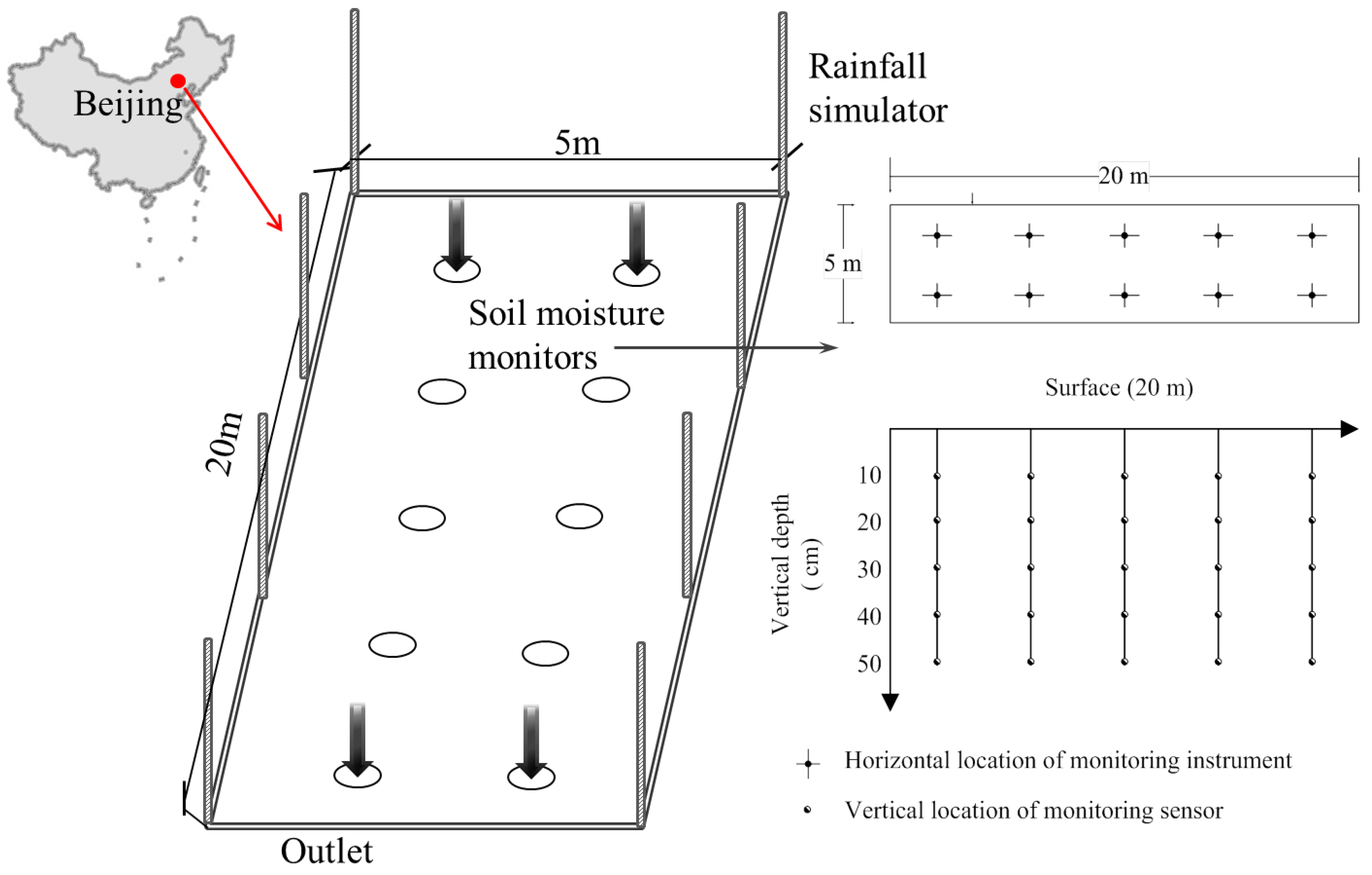
We conducted the field study on a natural hillslope (116°07′52″ E, 40°00′52″ N) located in the hilly area of YongDing River Basin, west of Beijing (Figure 1). This area is characterized by a warm temperate continental monsoon climate with four distinct seasons. The summers are hot and wet, and the winters are cold and dry. The annual mean temperature, and daily maximum and minimum temperatures are 11.7 °C, 40.2 °C, and −19.5 °C, respectively. The annual mean precipitation in the district is 568 mm (1981–2010) and it is unevenly distributed over the year. The rainfall in the rainy season (June–September) contributes about 81% of annual rainfall. During the observed period (from July 2016 to June 2017), the total rainfall was 628 mm, and the maximum rainfall amount in an event was 215 mm on 6 July. The largest peak rainfall intensity was 5 mm/min. Such heavy rain in the flood season was an extreme storm pattern and would induce soil erosion events, which made runoff easier and infiltration harder to be observed. Even if most of the precipitation concentrated in the flood season (from June to August), the natural rainfall-infiltration processes in the non-flood seasons (from September to May) were selected in this study, considering the importance to collect infiltration results. In the non-flood seasons, the total number of rainy days (>2 mm) was 16 days, and the mean rainfall intensity was 0.52 mm/min. The rainfalls in this period were sprinkles but lasted for longer time.

The natural-state experimental plots were located on the south-facing part of the hillslope, in a rectangle 20 m long and 5 m wide with an area of approximately 100 m² (Figure 1). The hillslope had an average gradient of 34% (corresponding slope is 19 degrees). The dominant vegetation was primary perennial herbs and shrubs. According to the China Soil Database, the loamy soil is the main soil type in the study sites, with mean bulk density of 1.4576 g/m³. The loamy soil properties, including texture (content of sand, silt, and clay), bulk density, saturated water content, saturated hydraulic conductivity, and the fitting parameters to soil water retention curve are described in

Table 1. Soil properties: texture (content of sand, silt, and clay), bulk density, saturated water content, saturated hydraulic conductivity, and the fitting parameters to soil water retention curve at this site.

Parameters	Texture	n	Sand	Silt	Clay	ρ	θn	D(θ)	α	Ks
			(%)	(%)	(%)	(g/cm3)	(cm3/cm3)		(/cm)	(m/d)
Values	loam	0.5	49.44	45.04	5.52	1.4576	0.5	0.001	5	0.000132

n: soil porosity; ρ: bulk density; θn: saturate soil water content; D(θ): hydraulic diffusivity; α: pore-disconnectedness index; Ks: saturated hydraulic conductivity.

.

2.2. Soil Moisture Measurement

Prior to observations, the experimental plot was bordered by cement bricks buried at a depth of 50 cm to avoid interference from outside the area. This brick border ensured that there was no water exchange between the inside and outside of the experimental area. A soil monitoring system was installed to record rainfall events and soil moisture conditions. This complex system covered ten points and five soil depths and comprised multiplex transducers. To measure inputs, two precipitation gauges (18 cm diameter, 70 cm height) were placed vertically on the hillslope. One was able to be moved to different places on the hillslope to reduce the error from interception by vegetation, and the other was fixed on the east side near the bottom of the brick-enclosed area. To characterize soil moisture in detail, eight EM50 instruments (each with a moisture sensor and temperature sensor) were placed randomly to subsurface on the hillslope, and deposition was measured at these eight positions every minute whether it was raining or not. The instruments monitored soil moisture and temperature at five depths (10, 20, 30, 40, and 50 cm). The soil moisture probe output was converted to volumetric soil moisture (m³/m³) ranging from 0 to 100% with accuracy of ±2%. Most infiltration models and equations assume that initial soil moisture is uniform among different depths, but in reality, initial water moisture is non-uniform in the natural soil profile. Monitoring instruments can record non-uniform initial water moisture during the infiltration process. The initial water moisture data recorded by the EM50 instruments were used to simulate the distribution of soil water during infiltration.

2.3. Theory

Experiments have shown that, in the absence of a water table, there are two basic patterns of soil-water distribution following infiltration [32]. The first is that soil moisture always decreases monotonically with depth and the water-content gradient across the wetting front gradually decreases as the front descends. In this case, the smaller the amount of infiltrated water, the faster the distribution rate. This condition occurs in fine-grained soils and small initial depths to the wetting front at the end of infiltration. The second pattern is the development of a “bulge” in soil moisture because of rapid gravitational drainage soon after infiltration ends, and this bulge persists as distribution progresses. A sharp wetting front is maintained, but the soil moistures above the bulge form a gradual “drying front” that is transitional to the field capacity. This situation occurs when the gravitational force is significant and hence, it is a characteristic of coarse-grained soils and deeper soil layers.

Following Hillel [33], we considered distribution first in completely wetted profiles, and then in partially wetted profiles. The process of distribution is governed by, and can be numerically modeled using, the Richards’ equation. The one-dimensional form of Richards’ [1] equation describes two items: sorption and gravity. Sorption is the horizontal infiltration of water into a partly but uniformly saturated soil when the movement of displaced air is unimpeded. Although this type of one-dimensional horizontal flow may not be very common in nature, the solution of this problem is of practical importance. Over the years, sorptivity has come to be considered as one of the more fundamental flow properties of a soil, and its relevance extends well beyond the phenomenon of sorption [34]. Sorptivity also arises naturally in the formulation of vertical infiltration capacity and in the formulation of different facets of rainfall infiltration [35,36,37]. Most natural soils have soil water diffusivity, which is strongly dependent on soil moisture [38]. Therefore, the results obtained in the following section with a linearized soil model may appear suspect at first. However, soil moisture-dependency is not always strong, so a linear model may still come close to describing the situation. Indeed, linearization simplifies the analysis considerably.

2.3.1. Governing Equations

Richards’ equation, as the basic theoretical equation for infiltration into a homogeneous porous medium, was derived by combining Darcy’s Law for vertical unsaturated flow with the conservation of mass [1]. Richards’ equation can be used as the basis for numerical modeling of infiltration, exfiltration, and distribution by specifying appropriate boundary and initial conditions, by dividing the soil into thin layers, and then applying the equation to each layer sequentially over small increments of time [39]. Tests have shown good agreement between the predictions of the numerically solved Richards’ equation and field and laboratory measurements [40]. However, because it is non-linear, there is no closed-form analytical solution except for highly simplified boundary conditions. Numerical solutions are not very useful for providing a conceptual overview of the ways in which various factors affect infiltration, and they are generally too computationally intensive to include in operational hydrological models. Thus, it is necessary to develop approximate analytical solutions to the Richards’ equation for specific situations, such as soil moisture content distribution and infiltration [41].

The movement of water after infiltration is complicated: upward- and downward-directed pressure gradients can develop in different parts of the profile due to drainage and evapotranspiration, and the effects of hysteresis can also be important [38]. There are many factors that determine the process of infiltration, but in this study, the following idealized condition is assumed: the block of soil is homogeneous to an indefinite depth; has a horizontal surface at which there is no evapotranspiration; and has soil moisture (θ) just prior to t = 0 that is also invariant at an initial value θ₀.

We assumed the validity of the Richards’ equation for flow in the unsaturated zone and used the Brooks-Corey [42] approximation for soil-water retention. Richard’s equation was written to include an evolving moisture content (θ). In idealized conditions, Richards’ equation can be described as follows:

$$-\frac{\partial \theta }{\partial t}=\nabla \cdot \left[-K\left(\theta \right)\cdot \nabla \mathsf{\psi }\right]$$

(1)

where t is time; $\nabla \mathsf{\psi }$ is a source–sink term, which includes x, y, and z as longitudinal, lateral, and vertical (positive downward) directions, respectively; $K\left(\theta \right)$ is the hydraulic conductivity; $\theta$ is volumetric soil moisture (ratio of water volume to soil volume), and the theoretical range of θ is from 0 (completely dry) to n (saturated, where n is soil porosity).

$$\theta =\frac{V_w}{V_s}$$

(2)

where $V_w$ is the volume of liquid water in the soil; $V_s$ is the total volume of soil.

$\nabla$ is the operator:

$$\nabla =\frac{\partial }{\partial x}\overrightarrow{i}+\frac{\partial }{\partial y}\overrightarrow{j}+\frac{\partial }{\partial z}\overrightarrow{k}$$

(3)

where $\overrightarrow{i}$, $\overrightarrow{j}$ and $\overrightarrow{k}$ are three unit vectors in the x, y, and z direction.

For the stratified soil layers, we considered only flows in the vertical direction, so the one-dimensional simplified Richards’ equation could be written as follows:

$$\frac{\partial \theta }{\partial t}=\frac{\partial }{\partial z}\left[K\left(\theta \right)\frac{\partial \mathsf{\psi }}{\partial z}\right]$$

(4)

As shown in Equation (3), Richards’ equation has two terms: one expressing the contribution of the suction gradient, and the other originating from the gravitational component of total potential. Whether one or the other term predominates depends on the initial and boundary conditions and on the stage of the process considered [33]. Diverse factors affect soil water distribution in soil layers at different depths. Therefore, the initial and boundary conditions should account for different factors affecting soil water distribution in different soil layers.

2.3.2. Modified Solution Equation with Parameters of Soil Properties for Upper Soil Layer

In Equation (3), hydraulic conductivity is determined largely by the size (cross-sectional area) of the pathways available for water transmission. In the upper soil layers, this size is determined by grain size and the degree of saturation. For a given soil, hydraulic conductivity increases non-linearly to its saturated value, $k_s$. The power-law equation is as follows:

$$K(\theta )=k_s{\left(\frac{\theta }{n}\right)}^{\alpha }$$

(5)

where $k_s$ is the hydraulic conductivity at saturation; α is the pore-disconnectedness index.

The hydraulic diffusivity $D\left(\theta \right)$ is defined as follows:

$$D\left(\theta \right)=K\left(\theta \right)\frac{\mathrm{d}{\mathsf{\psi }}_m}{d\theta }$$

(6)

where Ψ_m is water pressure head. Therefore, the solution of Equation (6) can be formulated as follows:

$$\frac{\partial \theta }{\partial t}=D\frac{{\partial }^2\theta }{\partial z^2}-\frac{\alpha }{n}{k}_s\frac{\partial \theta }{\partial z}$$

(7)

Assuming the following initial and boundary conditions:

$$\theta \left(z,t\right)|{}_{t=0}=\Delta \theta \cdot \delta \left(z-0\right)$$

(8)

where δ is the water potential difference between the depth of z and the surface. Integrating Equation (8) leads to:

$$\theta (z,t)=\frac{{\theta }_0}{\sqrt{\pi Dt}}\exp \left(-\frac{{\left(z-\frac{\alpha }{n}{k}_{s}t\right)}^2}{4Dt}\right)$$

(9)

2.3.3. Analytical Formulation with Slope for Deeper Soil Layer

Two directions have been commonly used for infiltration on the hillslope. The main direction is the direction normal to the slope surface [43], and the other is the vertical direction, which is taken as the divide [44]. We used Richards’ equation, which has the same coordinate system as Philip’s; therefore, it is more reasonable to use the direction defined by Philip [43].

Flow occurs in response to spatial gradients of mechanical potential energy, which has two components: gravitational potential energy and pressure potential energy [1]. For unsaturated soil, the hydraulic head $\mathsf{\psi }$ is defined as the sum of the water pressure head ${\mathsf{\psi }}_m$ and elevation head ${\mathsf{\psi }}_g$, so we have:

$$\mathsf{\psi }={\mathsf{\psi }}_m+{\mathsf{\psi }}_g.$$

(10)

Considering the effect of slope:

$${\mathsf{\psi }}_g=z\cdot \cos \beta$$

(11)

where β is the hillslope.

In Equation (3), assuming there is a uniform function for the water potential gradient ${\mathsf{\psi }}_m$ and soil moisture θ, and also for the hydraulic conductivity $K\left(\theta \right)$ and soil moisture θ, the relationship becomes:

$$\frac{\partial \theta }{\partial t}=\frac{\partial }{\partial z}\left[K\left(\theta \right)\frac{\mathrm{d}{\mathsf{\psi }}_m}{d\theta }\frac{\partial \theta }{\partial z}\right]+\cos \beta \cdot \frac{dK\left(\theta \right)}{dz}\frac{\partial \theta }{\partial z}$$

(12)

As mentioned above, hydraulic diffusivity $D\left(\theta \right)$ is defined using Equation (6), assuming the hydraulic conductivity $K\left(\theta \right)$ is a constant $k$, so $D\left(\theta \right)$ becomes constant and the following solution is obtained:

$$dK\left(\theta \right)/d\theta =k$$

(13)

where $k\left(\theta \right)$ is a constant of the hydraulic conductivity value.

The result is here approximated as follows:

$$\frac{\partial \theta }{\partial t}=D\frac{{\partial }^2\theta }{\partial z^2}+k\cdot \cos \beta \cdot \frac{\partial \theta }{\partial z}.$$

(14)

The infiltration into subsurface soil after precipitation is governed by Richards’ equation, but the boundary conditions are quite different in specific situations. In this study, we assumed the following linear initial and boundary conditions:

$$\{\begin{array}{l}\theta \left(z,0\right)={\theta }_0\\ \theta \left(0,t\right)={\theta }_n\\ \underset{x\to \infty }{\lim }\theta \left(z,t\right)={\theta }_0\end{array}$$

(15)

where θ₀ and θn are initial and saturate soil water content. The sum of soil moisture is defined as follows [28]:

$$\theta (z,t)={\theta }_1(z,t)+{\theta }_2(z,t).$$

(16)

For soil moisture, the following solution is obtained:

$$\frac{\theta -{\theta }_0}{{\theta }_n-{\theta }_0}=\frac{1}{2}\left[erfc\left(\frac{z-k\cdot \cos \beta \cdot t}{2\sqrt{Dt}}\right)+\exp \left(\cos \beta \cdot \frac{kz}{D}\right)\cdot erfc\left(\frac{z+k\cdot \cos \beta \cdot t}{2\sqrt{Dt}}\right)\right].$$

(17)

Here, erfc represents an iterated complementary error function [45].

The result is the soil moisture at any given time and depth in a semi-infinite unsaturated porous medium domain. The procedure described in this paper is valid for a specific series of successive soil-controlled phases of infiltration or any conditions specified by the given boundary conditions. The parameters needed in the equation are described above and shown in Table 1.

2.4. Data Statistics and Analysis

The performance of simulations was evaluated by root mean square error (RMSE), which was calculated as follows:

$$\mathrm{RMSE}=\sqrt{\frac{1}{N}\left({\displaystyle \sum _{i=1}^N{(\theta -\widehat{\theta })}^2}\right)}$$

(18)

where θ is the observed soil moisture at time t, $\widehat{\theta }$ is the estimated soil moisture at given time and depth, and N is the number of measurements.

To evaluate the accuracy of the predicted soil moisture of the equations, we calculated bias as follows:

$$\mathrm{Bias}=\frac{{\displaystyle {\sum }_i^N(\theta -\widehat{\theta })}}{N}.$$

(19)

The estimation results of the two equations were compared using Relative error (Re), which was calculated as follows:

$$\mathrm{Re}=\frac{\left|\theta -\widehat{\theta }\right|}{\theta }\times 100\%.$$

(20)

The simulation results were statistically analyzed using SPSS (version 18.0) software and Origin software 10.2.

3. Results

3.1. Temporal Analysis of Soil Moisture in Vertically Layered Soils

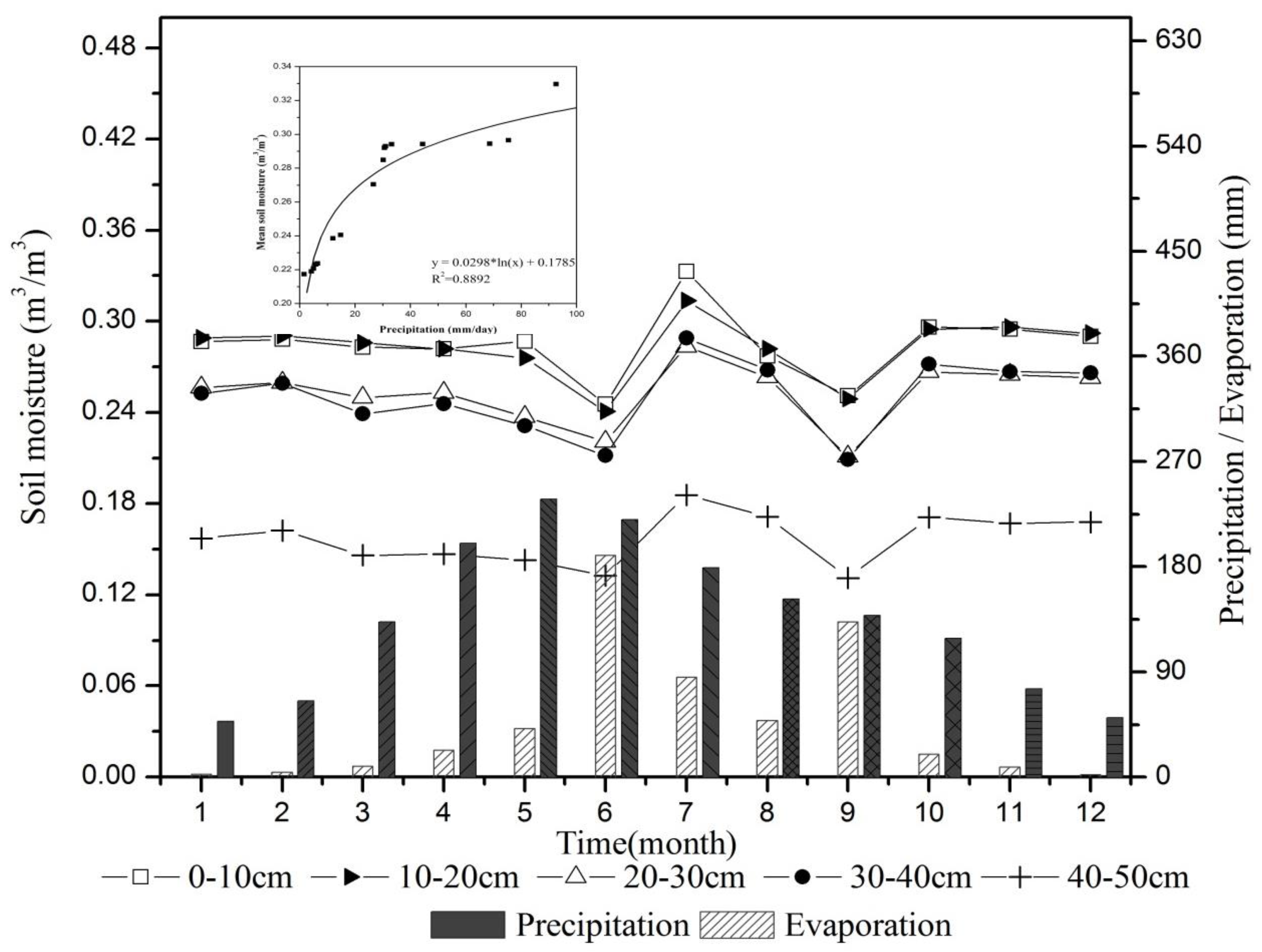
Soil moisture increased and decreased in response to seasonal climatic variations (Figure 2) and after recharge from individual precipitation events (Figure 3, Figure 4, Figure 5 and Figure 6). Precipitation was the main cause of variations in soil moisture over time. The response of soil moisture to precipitation is shown in Figure 2 (correlation coefficient between soil moisture and effective precipitation, 0.89). The correlogram indicated that soil moisture increased with increasing rainfall when the precipitation was less than 30 mm per day, but remained almost unchanged when the precipitation was greater than 30 mm per day. These results confirmed the process of infiltration.

The fluctuation of soil moisture was also influenced by other climate factors, such as evapotranspiration. As shown in Figure 2, the mean soil moisture values in June and September were lower than other summer months, which was attributed to the extreme high evapotranspiration in these two months.

Some previous studies obtained contrasting results. For example, Liao et al. [46] found that the highest mean soil moisture values in the year were in summer (from June to September). These findings provide meaningful information for choosing a better process of infiltration under drier soil conditions caused by larger rainfall amounts and stronger rainfall intensity.

The spatial variation in soil moisture in vertical directions was significant. The variation in soil moisture in different soil layers over time is also shown in Figure 2. In the upper soil layers (<30 cm), the soil moisture content decreased with precipitation events, and fluctuated and varied more dramatically than in the deeper soil layer (>30 cm).

Table 2. Temporal statistics (September 2016–August 2017) for mean soil moisture, the standard deviation, and the coefficient of variation in multiple soil layers.

Temporal Statistics	0–10 cm	10–20 cm	20–30 cm	30–40 cm	40–50 cm
Mean (%)	31.58%	30.83%	23.04%	24.65%	16.28%
Standard Deviation (SD)	0.037708	0.018525	0.006102	0.01508	0.015195
Coefficient of Variation (CV)	11.94%	6.01%	9.33%	6.12%	2.65%

shows the mean, standard deviation (SD), and coefficient of variation (CV) values for soil moisture content in multiple soil layers at observed points. The mean soil moisture from 10 to 50 cm remained unsaturated during most stages of the study period, but the soil moisture in each layer never approached the residual soil moisture. As soil moisture increased, the mean moisture showed a decreasing trend with values of 31.58%, 30.83%, 23.04%, 24.65%, and 16.28% at 0–10, 10–20, 20–30, 30–40, and 40–50-cm depths, respectively. As indicated by the SD and CV of soil moisture over time in multiple soil layers, there were larger changes in the spatial mean of soil moisture over time in the shallow soil layers, while soil moisture was more stable in the deeper layers.

3.2. Comparison of Simulation Results of Modified and Original Richards’ Equation for Two Soil Layers

Table 3. Simulation accuracy of modified equation and Richards’ Equation for top soil layer (10 cm).

Date	Root Mean Square Error (RMSE)		Bias		Relative Error
	Modified Equation	Richards’ Equation	Modified Equation	Richards’ Equation	Modified Equation	Richards’ Equation
2016/9/26	0.0057	0.0083	0.0052	−0.0053	2.41%	2.19%
2016/10/7	0.0108	0.0199	0.0090	0.0197	3.36%	7.47%
2016/11/21	0.0061	0.0050	0.0047	−0.0032	1.84%	1.18%
2017/3/24	0.0010	0.0080	0.0010	−0.0080	0.66%	5.20%
2017/4/13	0.0037	0.0066	0.0026	−0.0061	1.68%	3.75%
2017/5/13	0.0272	0.0428	0.0030	0.02342	1.06%	7.85%
Average	0.0091	0.0151	0.0042	0.0034	1.84%	4.61%

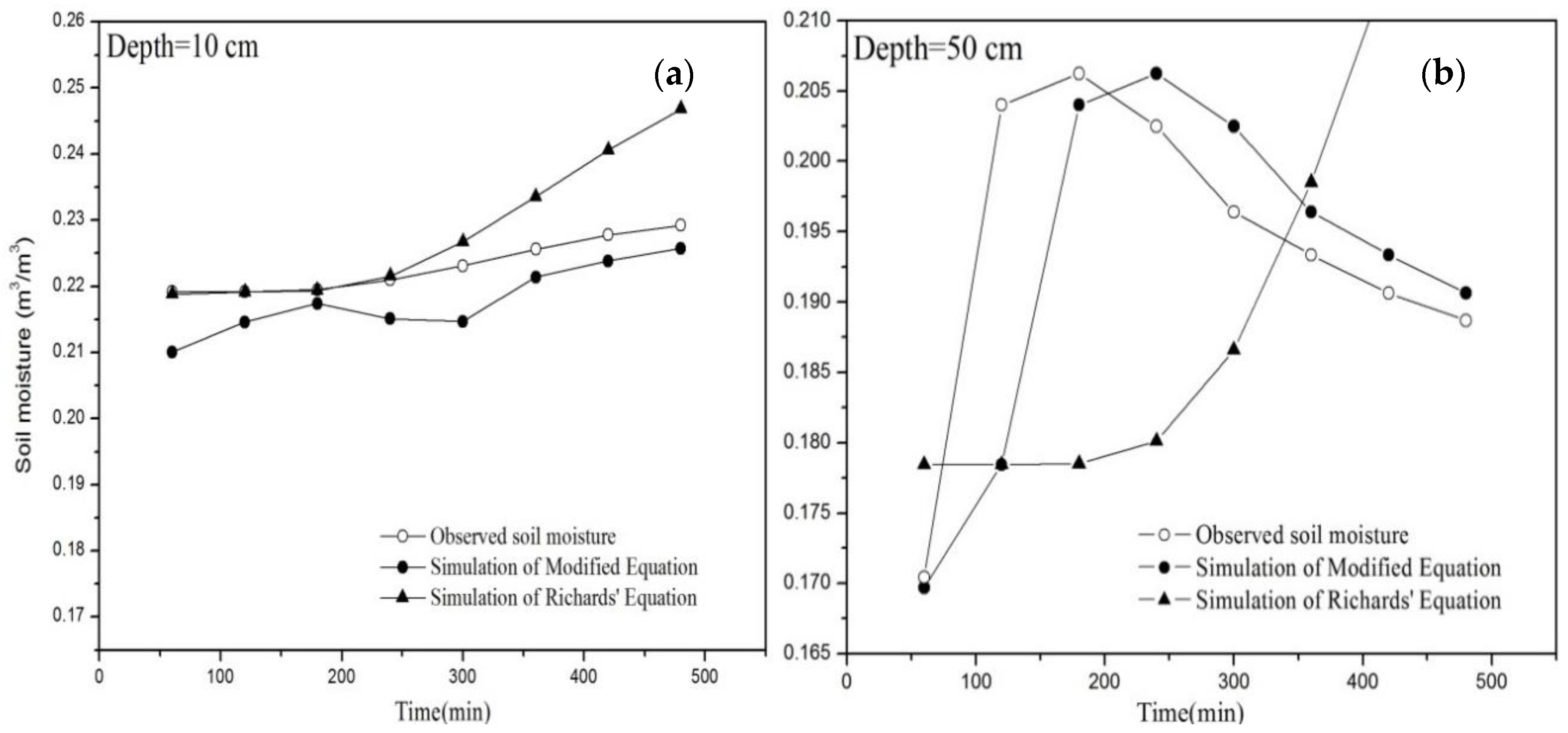
RMSE: the root mean square error.

and

Table 4. Simulation accuracy of modified equation and Richards’ Equation for deeper soil layers (50 cm).

Date	Root Mean Square Error		Bias		Relative Error
	Modified Equation	Richards’ Equation	Modified Equation	Richards’ Equation	Modified Equation	Richards’ Equation
2016/9/26	0.0100	0.0233	0.0024	0.0019	1.47%	1.98%
2016/10/7	0.0016	0.0150	0.0013	−0.0052	0.57%	1.84%
2016/11/21	0.0026	0.0063	0.0024	−0.0062	1.43%	3.63%
2017/3/24	0.0010	0.0080	0.0010	−0.0080	0.66%	5.20%
2017/4/13	0.0037	0.0066	0.0026	−0.0061	1.68%	3.75%
2017/5/13	0.0579	0.0569	0.0046	−0.0008	3.79%	1.57%
Average	0.0128	0.0194	0.0023	−0.0041	1.60%	2.99%

RMSE: the root mean square error.

compare the soil moisture simulation results between observed values and estimated values at two soil depths (10 and 50 cm) using the modified and original Richards’ equation. Six infiltration processes were selected in the study area from September 2016 to May 2017 during the rainy period. For the upper soil layers, the patterns of estimated soil moisture were similar to the measured patterns, but there was more severe bias when using the modified Richards’ equation. This was indicative of the uncertainty limits in the upper layer. The RMSE generated by the modified equation was between 0.0010 and 0.0272, while the Re was below 5% (see in Table 3). Hence, the modified Richards’ equation was more accurate than the original one. For the deeper soil layers, soil moisture fluctuated sharply and peaked 3 h after the rain stopped. The original Richards’ equation was insufficient to describe the distribution of soil moisture in the empirical case. The estimated soil moisture should have gradually fluctuated in a range as for the observed values, but the soil moisture estimated by the original Richards’ equation increased over time. The average value of RMSE, bias, and Re for the modified Richards’ equation were 0.0128, 0.0024, and 1.60%, respectively, indicating that it was more accurate than the original equation. Therefore, there were significant differences in observed soil moisture for two soil layers at the same points; while the modified Richards’ equation can reproduce the soil water content accurately for both of the two depths.

3.3. Spatiotemporal Variability in Soil Moisture Estimates

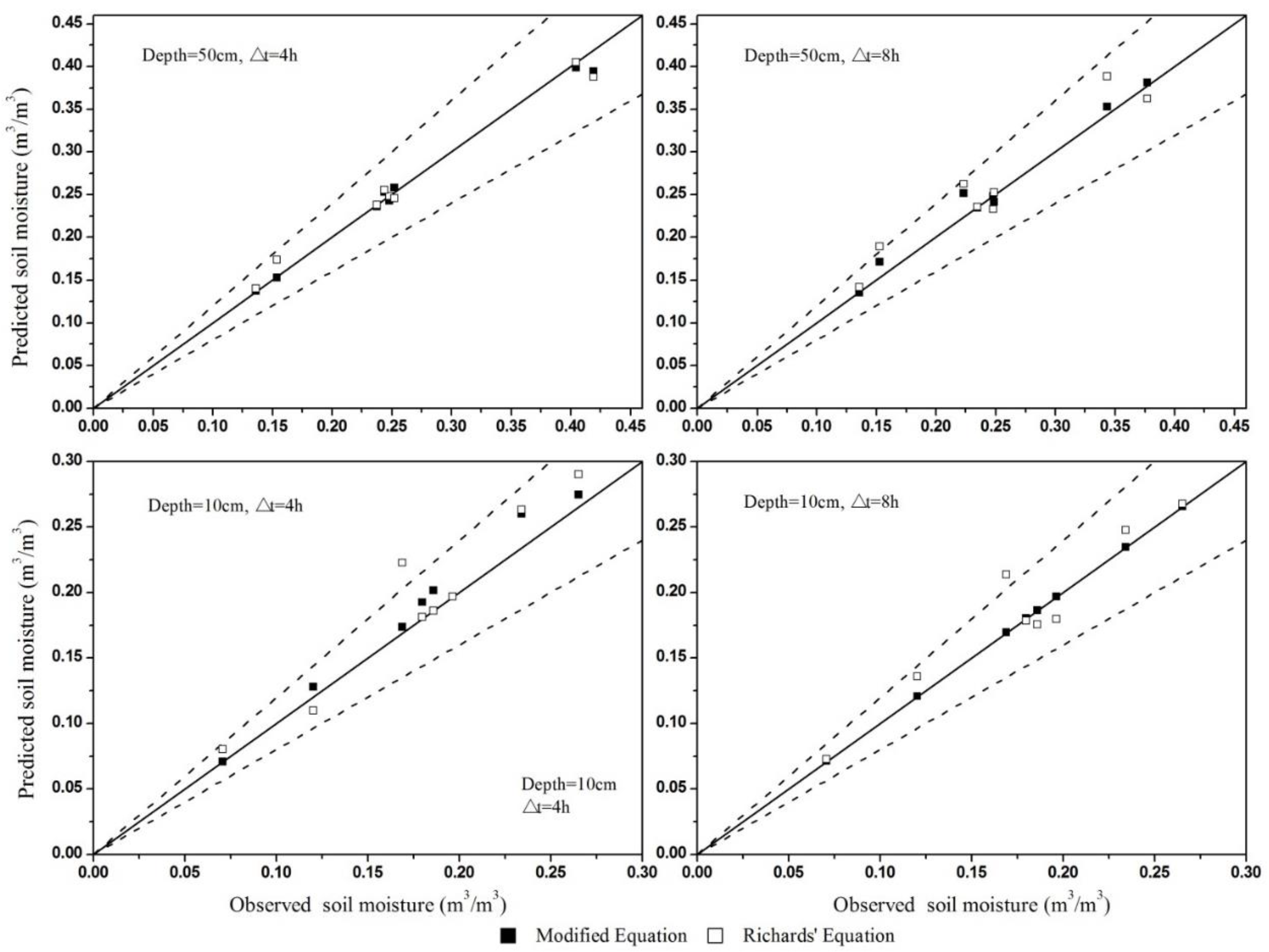
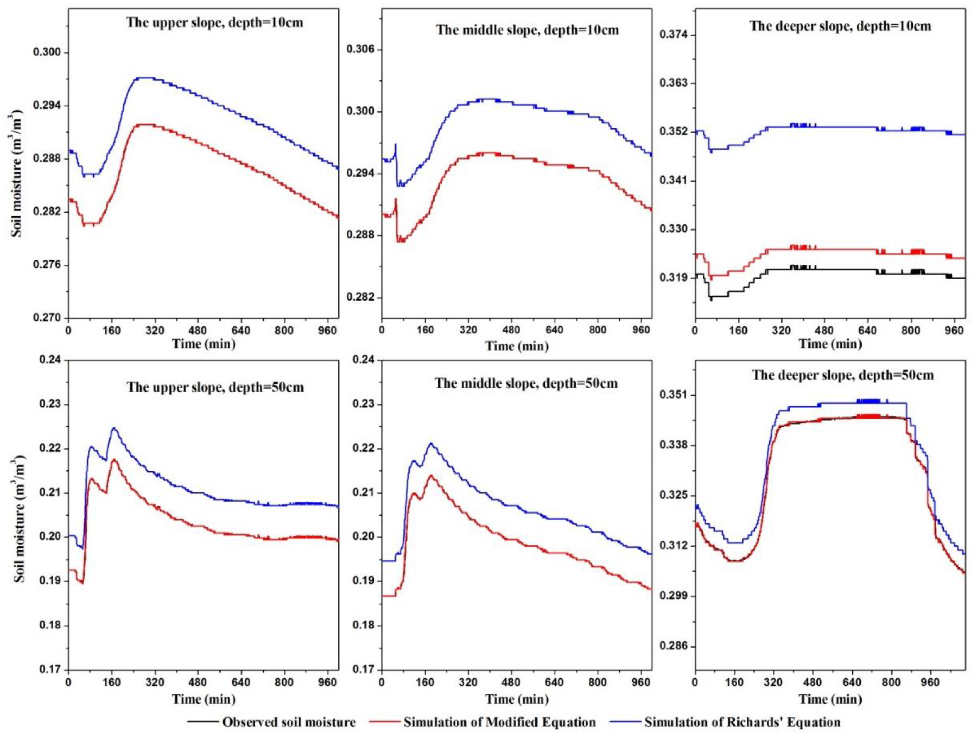
As shown in Figure 4, different uncertainty limits were specified for the two soil layers at eight points in the study plot. The observed soil moisture at the eight points in different slope positions are on the X-axis, and the results calculated with the two equations are on the Y-axis. To show the accuracy of the measured and estimated soil moisture values, two lines in the range of ±20% errors were plotted around the line of perfect agreement. At all sites, soil water content differed among different slope positions and depths, while the patterns of the fluctuations in soil moisture were similar to each other. The accuracy of the simulation results was less affected by the spatial variability on the hillslope during the study period. The soil moisture estimated using the modified Richards’ equation was generally more accurate than that estimated using the original Richards’ equation for both of two soil layers in the region. In addition, the simulation results of the modified Richards’ equation showed no spatial diversity in the deeper soil layer, so it did not improve the accuracy of the results for the deeper layer. In the deeper soil layer, the factor of slope affected the decomposition of gravity so that the simulation did not make sense for this layer. In contrast, the simulations for the upper soil layer did not have this source of interference. For the upper soil layer, the estimated soil moisture in the upper part and middle part of the slope fluctuated over time with little deviation from observation; while for the deeper part of the slope, the simulation showed relative large deviations (Figure 5). This result indicated that the original Richards’ equation lost its efficacy to describe soil moisture after infiltration in two-layered soils. Although there were some differences between the simulated and observed data for the lower part of the slope, the overall simulations were in a good agreement throughout the infiltration processes.

For both the upper and the deeper layers, the soil moisture estimated from the modified Richards’ equation in the infiltration process after two longer rainfall events separated by short intervals was closer to the observed values than were those calculated directly from the original Richards’ equation (Figure 5). Both equations produced higher estimates of soil moisture in the upper layer than the observed values. For the deeper soil layer, the simulation using the modified Richards’ equation showed better agreement with observed values. Overall, both equations could not accurately estimate soil moisture in the upper layer during longer rainy periods. The main reasons for these inaccuracies were the variations in physical variables under different natural conditions. The main reason for the high relative error of soil water estimates for the upper layer was that overland flow occurred over hillslope surfaces during infiltration, which is discussed later.

4. Discussion

4.1. Impact of Overland Flow on Simulations of Soil Moisture in Upper Soil Layer in Longer Rainy Periods

Based on the boundary conditions assumption, the improved Richards’ equation provided more accurate estimates of soil moisture than did the original Richards’ equation. However, the modified equation showed a limited ability to replicate the observed soil moisture traces in longer rainy periods and different spatial patterns of soil moisture. During infiltration, excess overland flow occurs when the rainfall rate is greater than the infiltration capacity, so that the excess water runs off over the surface. Overland flow is not a universally occurring phenomenon on a hillslope, and the prevalence of infiltration excess overland flow depends on the intensity of the precipitation [47]. Infiltration excess overland flow is the main mechanism of water movement when surfaces are relatively impermeable or when there is a higher rainfall rate with only a thin soil layer. It can also occur on other more permeable surfaces if the rainfall is sufficiently intense. Therefore, in the case shown in Figure 6, the two rainfall events separated by a short interval and the large rainfall amount and strong intensity led to overland flow. The soil moisture distribution in the upper layer was affected by the spatial variability of the infiltration excess overland flow.

During the second rainfall event, the initial soil moisture was close to the saturated state in the upper soil layer, and surface runoff occurred immediately after the start of the rainfall event according to the mechanism of saturation excess overland flow. In that case, the soil moisture at 10 cm depth estimated using the original and modified Richards’ equations became less accurate. These overland flow conditions in the shallow soil layers have implications for the prediction of factors controlling infiltration processes and soil moisture distribution. If the surface soil is almost saturated before infiltration or the intensity of precipitation is higher than the infiltration rate, then the precipitation water will be lost by overland flow. Therefore, the simulation results for the upper layer were larger than the observed values because the infiltration water was lost via overland flow during longer rainy periods.

4.2. Effect of Downslope Flow on Accuracy of Simulations in Different Slope Positions

As shown in Figure 5, there were discrepancies in the simulation results along the slope and estimates were more reliable for some parts of the slope than for others. This indicated that the values for environmental control factors in the current modified equation could not significantly improve the estimated results for the lower slope. It is possible that downslope flow occurred in the upper soil layer, causing errors in the simulation of the modified Richards’ equation. Philip’s solution [43] for infiltration on a hillslope included a parameter for downslope flow, that is, true lateral downslope flow that occurs on a hillslope. In this study, the hillslope was under a natural state with natural vegetation, and downslope flow could not be neglected, although the conditions for lateral downslope unsaturated flow have not been clearly identified [24]. For the empirical case described in the previous section, there were spatial patterns of soil moisture distribution along the hillslope from the upper part to the lower part at depths of 10 and 50 cm. That is, the soil moisture content was higher in the lower slope than in the middle and upper parts of the slope, consistent with the findings of Lv [24]. The results of simulations in different slope positions suggested that downslope flow parallel to the slope surface led to the space limitation. However, the effect of downslope flow on estimates of soil moisture cannot be concluded definitively. Another important aspect is the complexity of downslope flow. Under different natural environmental conditions (e.g., precipitation), soil moisture across a hillslope can show diverse responses. One source of uncertainty is the conditions for lateral downslope flow. Measuring the depth and direction of the flow is difficult, and subjoining the associated conceptualized parameters is equally difficult. Although the limitations of the equation resulting from the uncertainty of downslope flow were significant, they are beyond the purview of this study.

5. Conclusions

To estimate soil moisture for infiltration processes in layered soils, we propose a new modified version of Richards’ equation. We simulated the distribution of soil moisture on a hillslope using the modified and the original Richards’ equations, and compared the estimated results with measurements made at different depths and times. Our key findings are as follows:

• Although Richards’ equation is one of the most widely used infiltration equations in hydrological models, the original analytical solutions have a limited ability to estimate soil moisture traces during infiltration on a hillslope.
• The spatial–temporal variations in soil moisture are controlled by diverse environmental control factors, such as hillslope and soil properties. However, these factors are difficult to express using the original Richards’ equation because of the difficulty in summarizing the related parameters. As far as we know, this is the first attempt to express environmental factors using in situ layered parameters in the infiltration equation.
• The simulation results calculated by the modified Richards’ equation with layered parameters were better than those calculated by the original equation. However, the bias between the simulations using the modified Richards’ equation and the observed values was higher for the upper soil layers. The accuracy of simulations varied depending on the slope position and the length of the rainy period, because of the effects of lateral downslope flow and overland flow during infiltration.

The results of this study showed that estimates of soil moisture on a hillslope were improved by incorporating analytical solutions that consider different environmental controls in a modified Richards’ equation. The modified equation provides a new in-layered method to reproduce soil water distribution and can be applied in hydrological process models for use in research on water resources and soil erosion. In further research on this topic, several other control factors should be taken into account to improve the performance of an infiltration equation for estimating soil moisture along hillslopes and in multiple soil layers.

References

- Richards, L.A. Capillary conduction of liquids through porous mediums. Phys. J. Gen. Appl. Phys. 1931, 1, 318–333. [Google Scholar] [CrossRef]
- Koster, R.D.; Dirmeyer, P.A.; Guo, Z.C.; Bonan, G.; Chan, E.; Cox, P.; Gordon, C.T.; Kanae, S.; Kowalczyk, E.; Lawrence, D.; et al. Regions of strong coupling between soil moisture and precipitation. Science 2004, 305, 1138–1140. [Google Scholar] [CrossRef] [PubMed]
- Laio, F.; Porporato, A.; Ridolfi, L.; Rodriguez-Iturbe, I. Plants in water-controlled ecosystems: Active role in hydrologic processes and response to water stress—II. Probabilistic soil moisture dynamics. Adv. Water Resour. 2001, 24, 707–723. [Google Scholar] [CrossRef]
- Lewis, M.R. The rate of infiltration of water in irrigation practice. Trans. Am. Geophys. Union 1937, 18, 361–368. [Google Scholar] [CrossRef]
- Reeves, M.; Miller, E.E. Estimating infiltration for erratic rainfall. Water Resour. Res. 1975, 11, 102–110. [Google Scholar] [CrossRef]
- Baron, G. Abramowitz, A-handbook of mathematical functions. Computing 1967, 2, 169. [Google Scholar] [CrossRef]
- Bruce, R.R.; Thomas, A.W.; Whisler, F.D. Prediction of infiltration into layered field soils in relation to profile characteristics. Trans. Asae 1976, 19, 693–698. [Google Scholar] [CrossRef]
- Wang, G.; Fang, Q.; Wu, B.; Yang, H.; Xu, Z. Relationship between soil erodibility and modeled infiltration rate in different soils. J. Hydrol. 2015, 528, 408–418. [Google Scholar] [CrossRef]
- Xue, B.-L.; Wang, L.; Yang, K.; Tian, L.; Qin, J.; Chen, Y.; Zhao, L.; Ma, Y.; Koike, T.; Hu, Z.; et al. Modeling the land surface water and energy cycles of a mesoscale watershed in the central Tibetan Plateau during summer with a distributed hydrological model. J. Geophys. Res. Atmos. 2013, 118, 8857–8868. [Google Scholar] [CrossRef] [Green Version]
- Rossi, M.J.; Ares, J.O. Overland flow from plant patches: Coupled effects of preferential infiltration, surface roughness and depression storage at the semiarid Patagonian Monte. J. Hydrol. 2016, 533, 603–614. [Google Scholar] [CrossRef]
- Botter, G.; Porporato, A.; Rodriguez-Iturbe, I.; Rinaldo, A. Basin-scale soil moisture dynamics and the probabilistic characterization of carrier hydrologic flows: Slow, leaching-prone components of the hydrologic response. Water Resour. Res. 2007, 43. [Google Scholar] [CrossRef] [Green Version]
- Heathman, G.C.; Larose, M.; Cosh, M.H.; Bindlish, R. Surface and profile soil moisture spatio-temporal analysis during an excessive rainfall period in the Southern Great Plains, USA. Catena 2009, 78, 159–169. [Google Scholar] [CrossRef]
- Chu, S.T. Infiltration during an unsteady rain. Water Resour. Res. 1978, 14, 461–466. [Google Scholar] [CrossRef]
- Xue, B.-L.; Wang, L.; Li, X.; Yang, K.; Chen, D.; Sun, L. Evaluation of evapotranspiration estimates for two river basins on the Tibetan Plateau by a water balance method. J. Hydrol. 2013, 492, 290–297. [Google Scholar] [CrossRef]
- Rodriguez-Iturbe, I.; D’Odorico, P.; Porporato, A.; Ridolfi, L. On the spatial and temporal links between vegetation, climate, and soil moisture. Water Resour. Res. 1999, 35, 3709–3722. [Google Scholar] [CrossRef] [Green Version]
- Wang, G.; Jiang, H.; Xu, Z.; Wang, L.; Yue, W. Evaluating the effect of land use changes on soil erosion and sediment yield using a grid-based distributed modelling approach. Hydrol. Process. 2012, 26, 3579–3592. [Google Scholar] [CrossRef]
- Zhou, Q.; Driscoll, C.T.; Moore, S.E.; Kulp, M.A.; Renfro, J.R.; Schwartz, J.S.; Cai, M.; Lynch, J.A. Developing Critical Loads of Nitrate and Sulfate Deposition to Watersheds of the Great Smoky Mountains National Park, USA. Water Air Soil Pollut. 2015, 226, 255. [Google Scholar] [CrossRef]
- Martinez-Fernandez, J.; Ceballos, A. Mean soil moisture estimation using temporal stability analysis. J. Hydrol. 2005, 312, 28–38. [Google Scholar] [CrossRef]
- Huang, X.; Shi, Z.H.; Zhu, H.D.; Zhang, H.Y.; Ai, L.; Yin, W. Soil moisture dynamics within soil profiles and associated environmental controls. Catena 2016, 136, 189–196. [Google Scholar] [CrossRef]
- Gomez-Plaza, A.; Martinez-Mena, M.; Albaladejo, J.; Castillo, V.M. Factors regulating spatial distribution of soil water content in small semiarid catchments. J. Hydrol. 2001, 253, 211–226. [Google Scholar] [CrossRef]
- Takagi, K.; Lin, H.S. Changing controls of soil moisture spatial organization in the Shale Hills Catchment. Geoderma 2012, 173, 289–302. [Google Scholar] [CrossRef]
- Western, A.W.; Bloschl, G. On the spatial scaling of soil moisture. J. Hydrol. 1999, 217, 203–224. [Google Scholar] [CrossRef]
- Morbidelli, R.; Saltalippi, C.; Flammini, A.; Rao, S.G. Role of slope on infiltration: A review. J. Hydrol. 2018, 557, 878–886. [Google Scholar] [CrossRef]
- Lv, M.; Hao, Z.; Liu, Z.; Yu, Z. Conditions for lateral downslope unsaturated flow and effects of slope angle on soil moisture movement. J. Hydrol. 2013, 486, 321–333. [Google Scholar] [CrossRef]
- Kim, H.J.; Sidle, R.C.; Moore, R.D. Shallow lateral flow from a forested hillslope, Influence of antecedent wetness. Catena 2005, 60, 293–306. [Google Scholar] [CrossRef]
- Sun, H.; Meerschaert, M.M.; Zhang, Y.; Zhu, J.; Chen, W. A fractal Richards’ equation to capture the non-Boltzmann scaling of water transport in unsaturated media. Adv. Water Resour. 2013, 52, 292–295. [Google Scholar] [CrossRef] [PubMed] [Green Version]
- Corradini, C.; Melone, F.; Smith, R.E. Modeling local infiltration for a two-layered soil under complex rainfall patterns. J. Hydrol. 2000, 237, 58–73. [Google Scholar] [CrossRef]
- Menziani, M.; Pugnaghi, S.; Vincenzi, S. Analytical solutions of the linearized Richards equation for discrete arbitrary initial and boundary conditions. J. Hydrol. 2007, 332, 214–225. [Google Scholar] [CrossRef]
- Green, W.H.; Ampt, G.A. Studies on soil physics Part I—The flow of air and water through soils. J. Agric. Sci. 1911, 4, 1–24. [Google Scholar]
- Philip, J.R. Theory of Infiltration. Adv. Hydrosci. 1969, 5, 215–296. [Google Scholar]
- Wang, Y.; Hu, W.; Zhu, Y.; Shao Ma Xiao, S.; Zhang, C. Vertical distribution and temporal stability of soil water in 21-m profiles under different land uses on the Loess Plateau in China. J. Hydrol. 2015, 527, 543–554. [Google Scholar] [CrossRef] [Green Version]
- Horton, R.E. Analysis of Runoff-Plot Experiments With Varying Infiltration-Capacity. Eos Trans. Am. Geophys. Union 1939, 20, 693–711. [Google Scholar] [CrossRef]
- Hillel, D. A descriptive theory of fingering during infiltration into layered soils. Soil Sci. 1988, 146, 207–217. [Google Scholar] [CrossRef]
- Philip, J.R. Sorption and infiltration in heterogeneous media. Aust. J. Soil Res. 1967, 5, 1–10. [Google Scholar] [CrossRef]
- Talsma, T.; Parlange, J.Y. One-dimensional vertical infiltration. Aust. J. Soil Res. 1972, 10, 143–150. [Google Scholar] [CrossRef]
- Clothier, B.E.; White, I. Measurement of sorptivity and soil-water diffusivity in the field. Soil Sci. Soc. Am. J. 1981, 45, 241–245. [Google Scholar] [CrossRef]
- Cook, F.J.; Broeren, A. Six methods for determining sorptivity and hydraulic conductivity with disc permeameters. Soil Sci. 1994, 157, 2–11. [Google Scholar] [CrossRef]
- Parlange, J.Y. Theory of water-movement in soils: 1. One-dimensional absorption. Soil Sci. 1971, 111, 134–137. [Google Scholar] [CrossRef]
- Rathfelder, K.; Abriola, L.M. Mass conservative numerical-solutions of the head-based richards equation. Water Resour. Res. 1994, 30, 2579–2586. [Google Scholar] [CrossRef]
- Haverkamp, R.; Vauclin, M.; Touma, J.; Wierenga, P.J.; Vachaud, G. Comparison of numerical-simulation models for one-dimensional infiltration. Soil Sci. Soc. Am. J. 1977, 41, 285–294. [Google Scholar] [CrossRef]
- Su, L.; Wang, J.; Qin, X.; Wang, Q. Approximate solution of a one-dimensional soil water infiltration equation based on the Brooks-Corey model. Geoderma 2017, 297, 28–37. [Google Scholar] [CrossRef]
- Brooks, R.H.; Corey, A.T. Properties of porous media affecting fluid flow. J. Irrig. Drain. Div. 1966, 92, 61–88. [Google Scholar]
- Philip, J.R. Hillslope infiltration—Planar slopes. Water Resour. Res. 1991, 27, 109–117. [Google Scholar] [CrossRef]
- Jackson, C.R. Hillslope infiltration and lateral downslope unsaturated flow. Water Resour. Res. 1992, 28, 2533–2539. [Google Scholar] [CrossRef]
- Abramowitz, M.; Stegun, I.A.; Miller, D. Handbook of Mathematical Functions With Formulas, Graphs and Mathematical Tables. J. Appl. Mech. 1965, 32, 239. [Google Scholar] [CrossRef]
- Liao, K.; Zhou, Z.; Lai, X. Evaluation of different approaches for identifying optimal sites to predict mean hillslope soil moisture content. J. Hydrol. 2017, 547, 10–20. [Google Scholar] [CrossRef]
- Smith, R.E.; Chery, D.L. Rainfall excess model from soil-water flow theory. J. Hydraul. Div. Asce 1975, 101, 404–406. [Google Scholar]
Figure 1.
Location of observation station and schematic diagram of monitoring instrument distribution.
Figure 2.
Time series of precipitation, evaporation and mean soil moisture at four soil depths.
Figure 3.
Comparison between observed and simulated soil moisture by the modified Richards’ equation and original Richards’ equation (a) at the depth of 10 cm and (b) at the depth of 50 cm.
Figure 4.
Comparison of simulated and observed soil moisture at various measurement points and soil depths.
Figure 5.
Comparisons of the simulation results among different slope position. The depth is from 10 to 50 cm.
Figure 6.
Estimated and observed soil moisture at different depths for two rainfall events with short intervals.