Investigating the Dynamic Influence of Hydrological Model Parameters on Runoff Simulation Using Sequential Uncertainty Fitting-2-Based Multilevel-Factorial-Analysis Method


Abstract
:1. Introduction
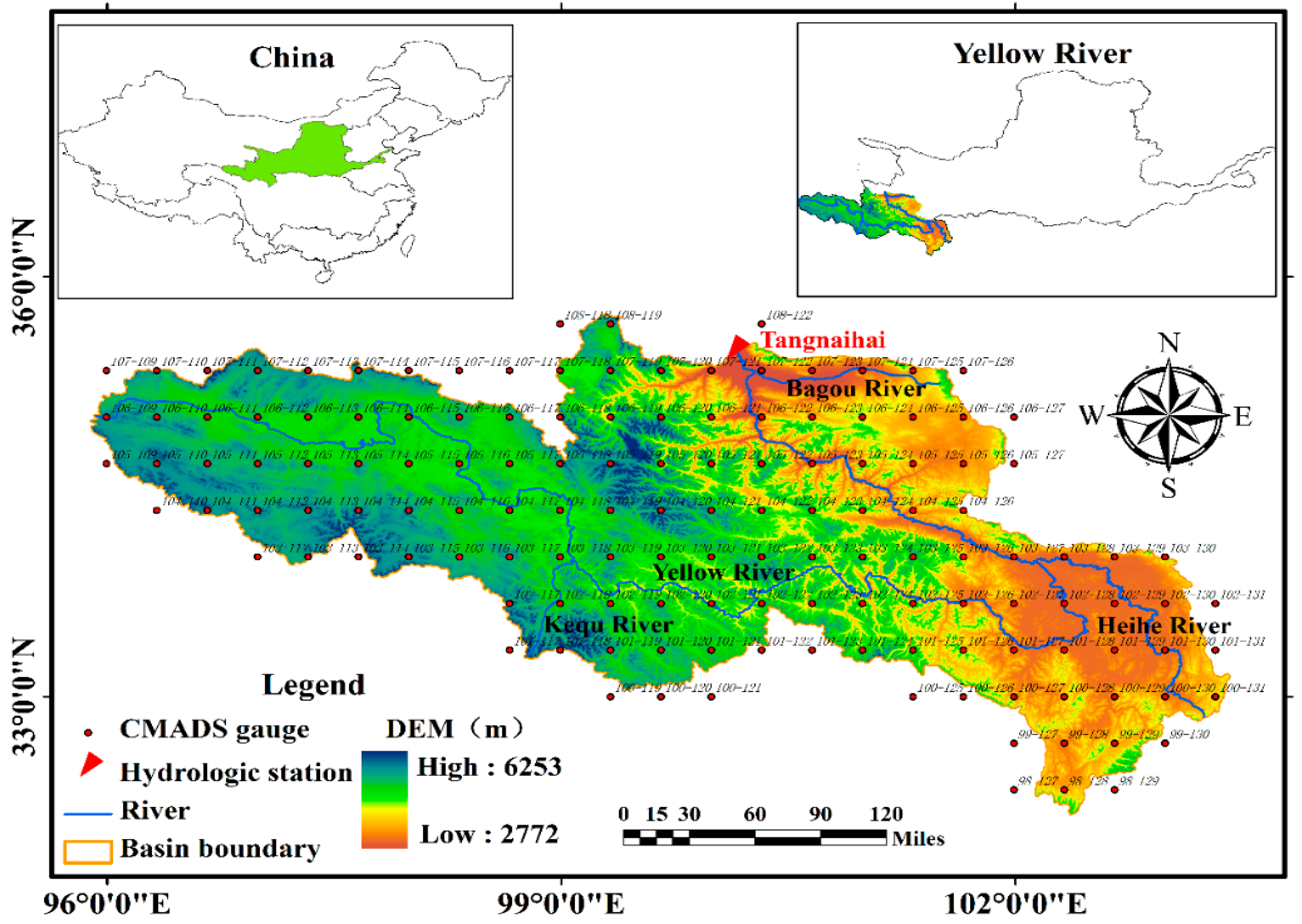
2. Study Area
3. Methodology
3.1. Construction of the Soil and Water Assessment Tool Model
3.2. Parameter Sensitivity Analysis
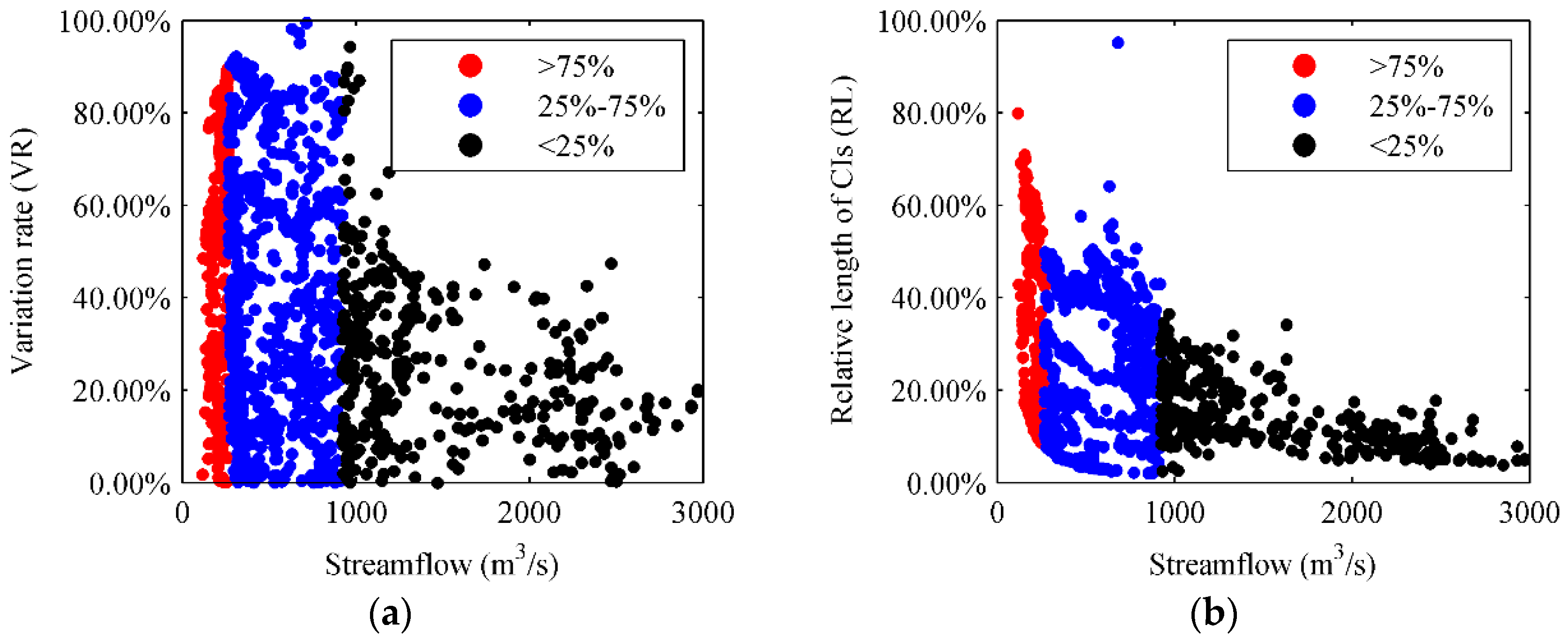
3.3. Parameter Uncertainty Evaluation Index
3.4. Multilevel Factorial Analysis
4. Results and Discussion
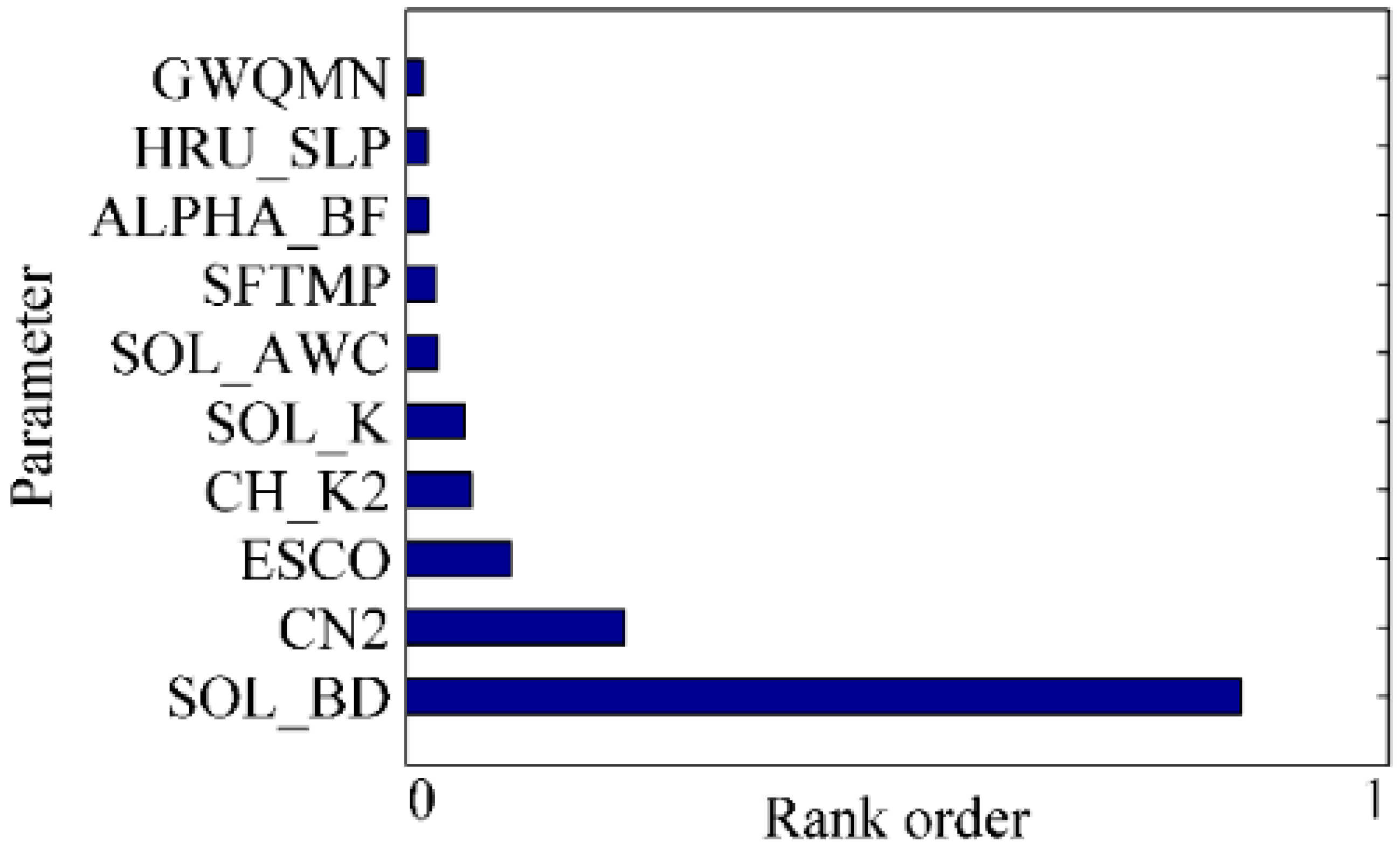
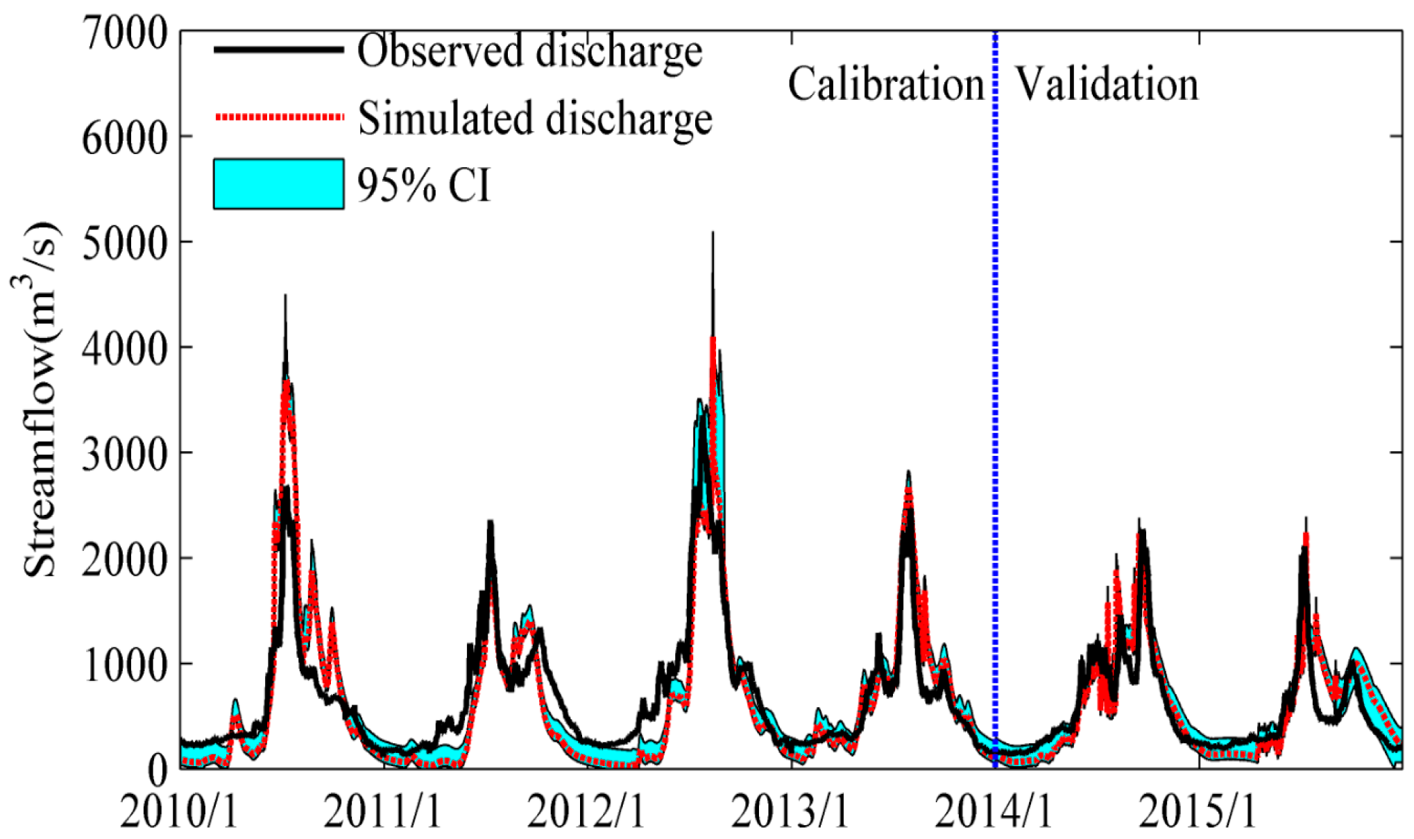
4.1. Parameter Sensitivity Analysis, Calibration, and Verification of Model
4.2. Multilevel Factorial Analysis and Dynamic Changes in Parameter Sensitivity
4.3. The Individual and Interactive Effects of Parameters on the Hydrologic Model Output in Different Periods
4.3.1. The Statistically Significant Individual and Interaction Effects on Runoff Simulation in Non-Flood Period
4.3.2. The Statistically Significant Individual and Interaction Effects on the Runoff Simulation in the Pre-Flood Period
4.3.3. The Statistically Significant Individual and Interaction Effects on the Runoff Simulation in the Flood Period
4.3.4. The Statistically Significant Individual and Interaction Effects on the Runoff Simulation in the Post-Flood Period
4.3.5. Contributions of Parameter Individual and Interaction Effects for the Runoff Simulation in Four Periods
5. Conclusions
- (1)
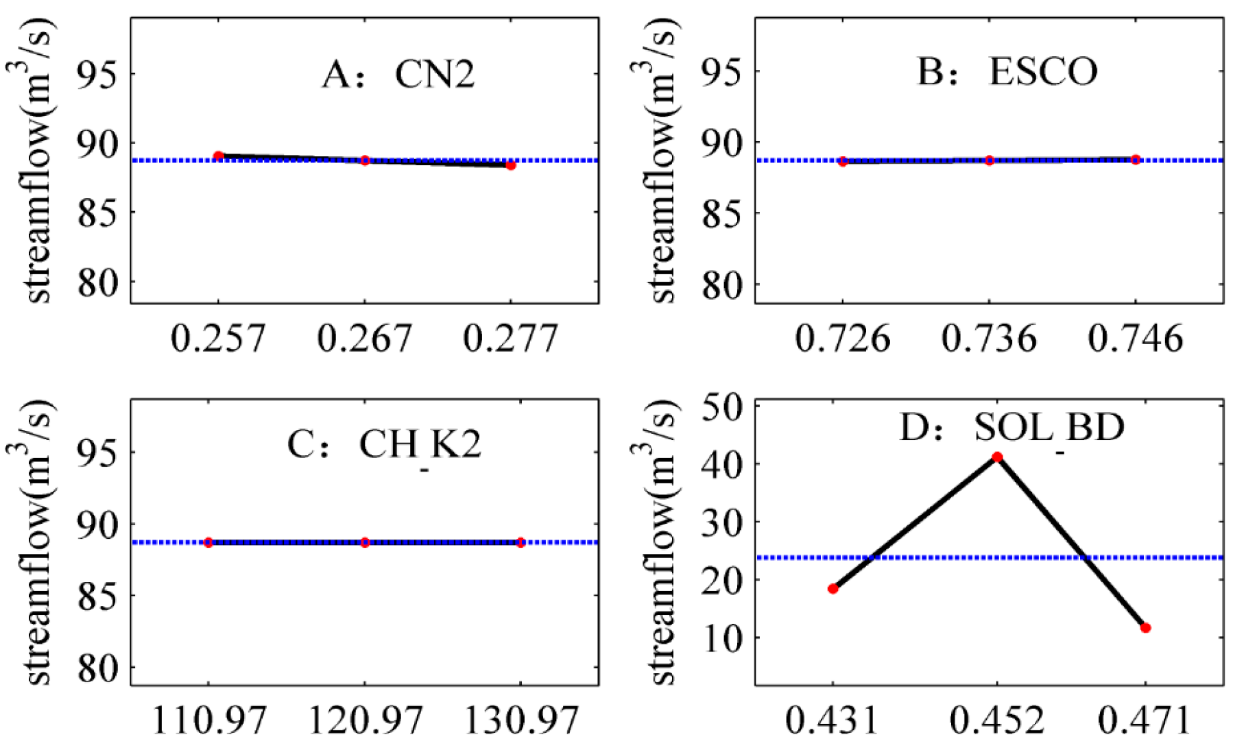
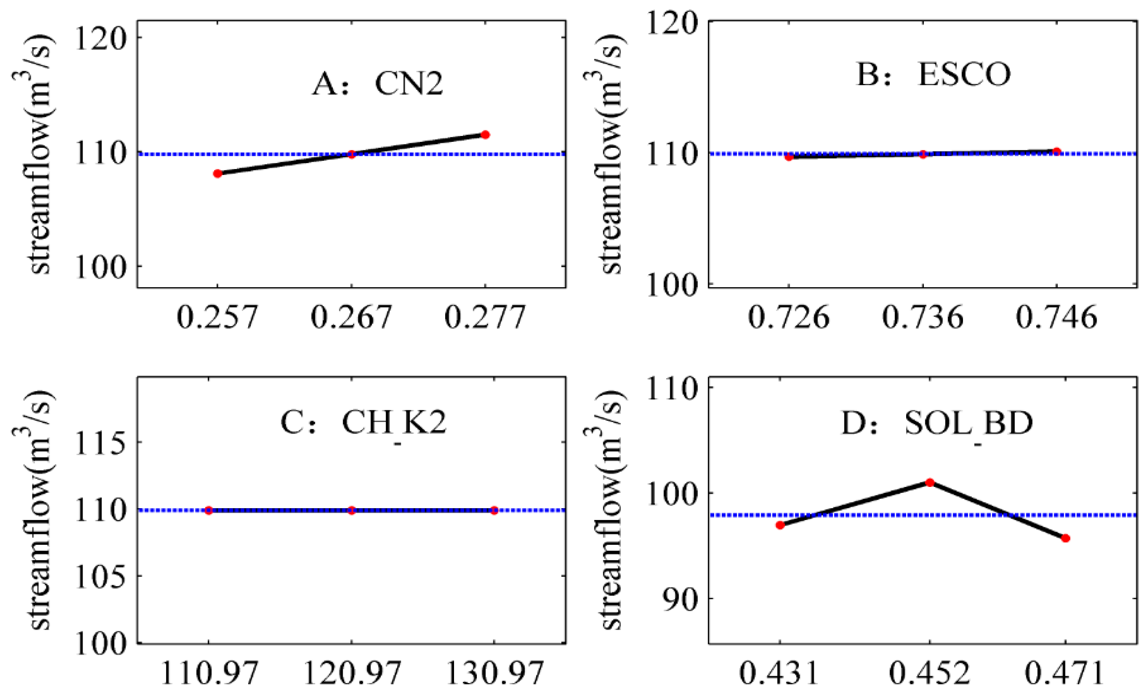
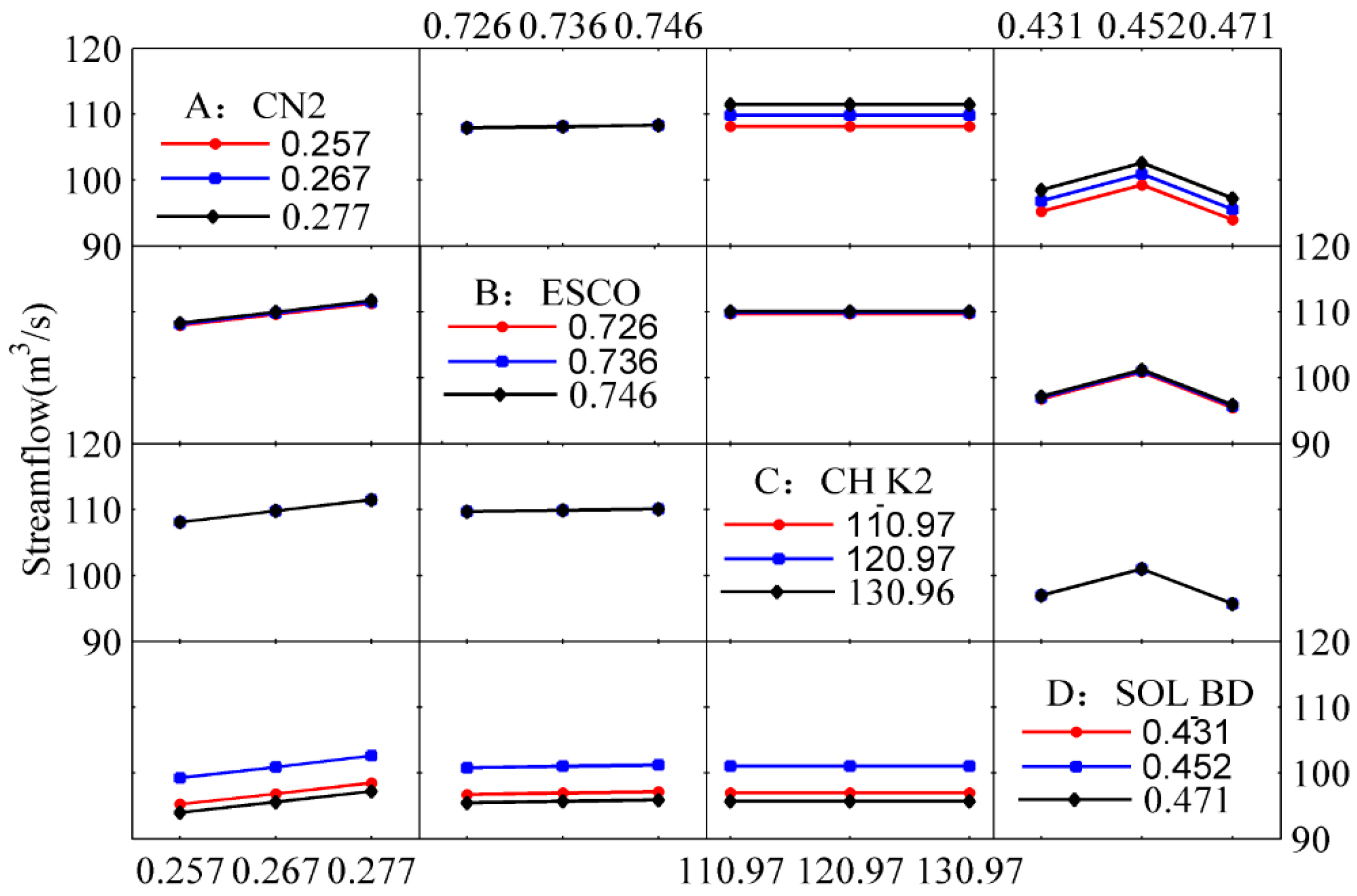
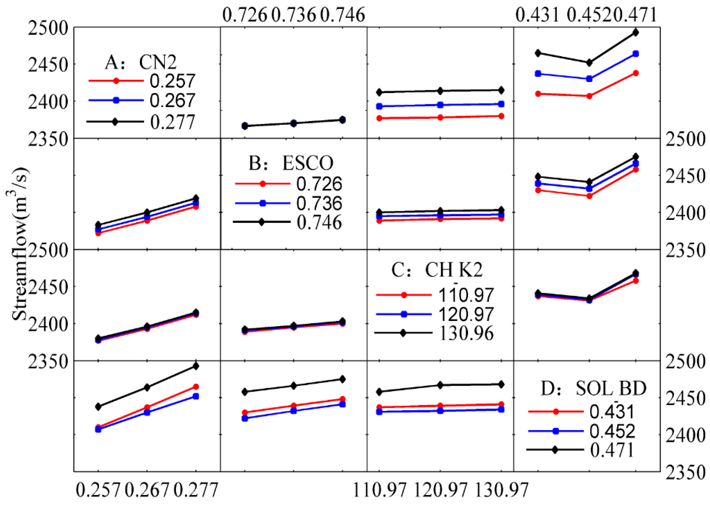
- The influence of parameters CN2, ESCO, CH_K2, and SOL_BD (i.e., A, B, C, and D, respectively) on the runoff simulation is significant in different periods (Figure 2, Table 3, Table 4, Table 5 and Table 6). In general, the linear individual effects of factors A, B, and D, as well as the AD interaction effects, are thus significant, while the others have little influence on the response.
- (2)
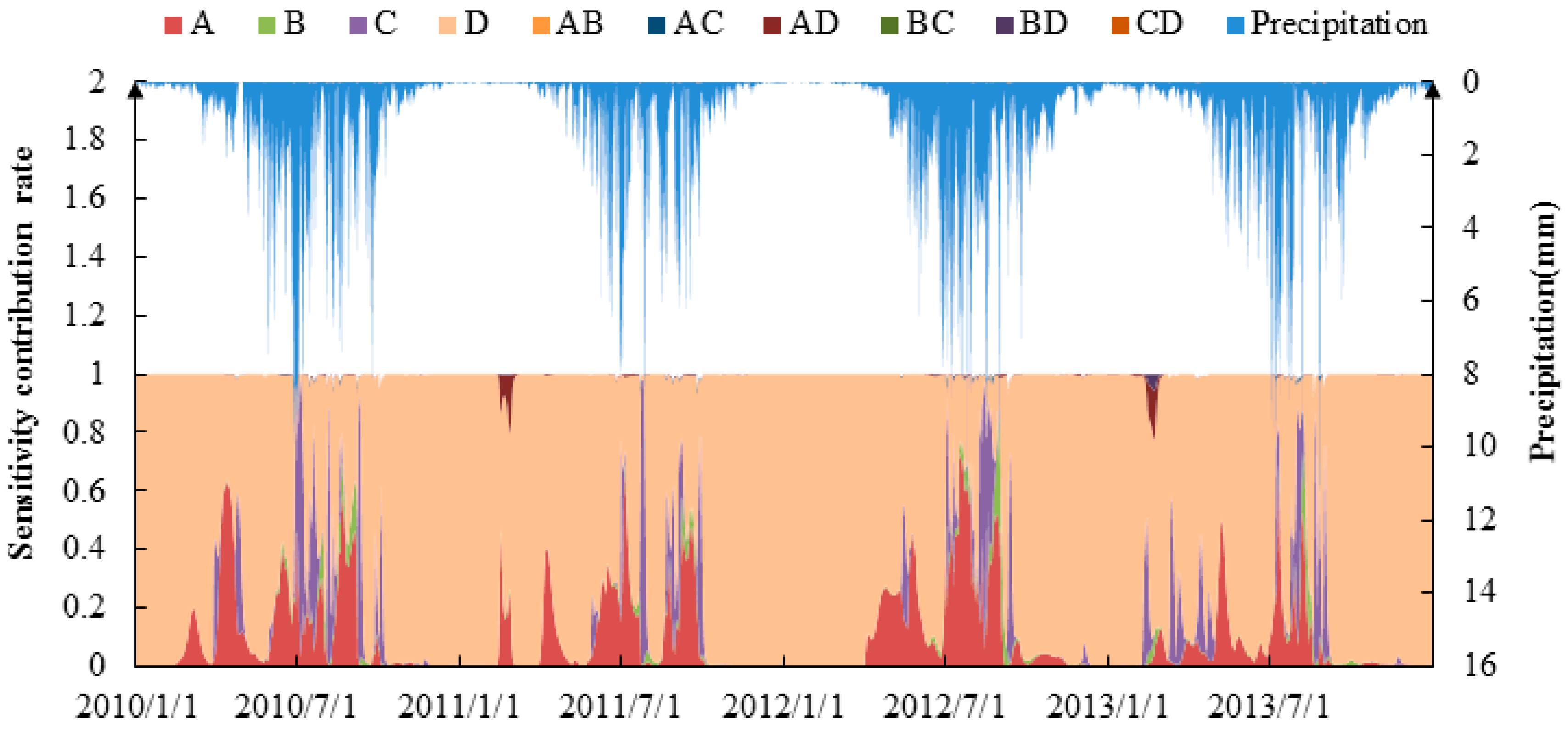
- The contributions of different parameters to the runoff simulation are different in different periods (Figure 14). The effect of soil bulk density (D) on the runoff simulation is significant in four periods, contributing 0.99, 0.73, 0.30, and 0.97, respectively. The effect of the initial SCS runoff curve number (A) on the runoff simulation is significant in the non-flood and flood periods, contributing 0.26 and 0.60, respectively.
- (3)
- The interaction effects of parameters on runoff simulation are significant in the flood period. Take parameters A and D as an example: The changes differ across the three levels of parameter D, depending on the level of parameter A. The slope curve is distinctly different between parameters A and D. This reveals the interaction of A and D has a significant influence on the runoff simulation. Therefore, the parameter interaction must be emphasized in flood periods.
- (4)
- In essence, the soil bulk density moisture content and infiltration-excess runoff production are important water inputs for the hydrological system in the source region of the Yellow River. It is further explained that soil bulk density will affect the loss of surface runoff and river recharge groundwater.
Supplementary Materials
Author Contributions
Funding
Conflicts of Interest
References
- Joseph, J.F.; Guillaume, J.H. Using a parallelized MCMC algorithm in R to identify appropriate likelihood functions for SWAT. Environ. Model. Softw. 2013, 46, 292–298. [Google Scholar] [CrossRef]
- Gashaw, T.; Tulu, T.; Argaw, M.; Worqlul, A.W. Modeling the hydrological impacts of land use/land cover changes in the Andassa watershed, Blue Nile Basin, Ethiopia. Sci. Total Environ. 2018, 619, 1394–1408. [Google Scholar] [CrossRef] [PubMed]
- Her, Y.; Chaubey, I.; Frankenberger, J.; Jeong, J. Implications of spatial and temporal variations in effects of conservation practices on water management strategies. Water Manag. 2017, 180, 252–266. [Google Scholar] [CrossRef]
- Vilaysane, B.; Takara, K.; Luo, P.; Akkharath, I.; Duan, W. Hydrological Stream Flow Modelling for Calibration and Uncertainty Analysis Using SWAT Model in the Xedone River Basin, Lao PDR. Procedia Environ. Sci. 2015, 28, 380–390. [Google Scholar] [CrossRef]
- Li, Z.L.; Shao, Q.X.; Xu, Z.X.; Cai, X.T. Analysis of parameter uncertainty in semi-distributed hydrological models using bootstrap method: A case study of SWAT model applied to Yingluoxia watershed in northwest China. J. Hydrol. 2010, 385, 76–83. [Google Scholar] [CrossRef]
- Ficklin, D.L.; Barnhart, B.L. SWAT hydrologic model parameter uncertainty and its implications for hydroclimatic projections in snowmelt-dependent watersheds. J. Hydrol. 2014, 519, 2081–2090. [Google Scholar] [CrossRef]
- Wu, Y.; Liu, S. Automating calibration, sensitivity and uncertainty analysis of complex models using the R package Flexible Modeling Environment (FME): SWAT as an example. Environ. Model. Softw. 2012, 317, 99–109. [Google Scholar] [CrossRef]
- Zhang, D.; Chen, X.; Yao, H.; James, A. Moving SWAT model calibration and uncertainty analysis to an enterprise Hadoop-based cloud. Environ. Model. Softw. 2016, 84, 140–148. [Google Scholar] [CrossRef]
- Kouchi, D.H.; Esmaili, K.; Faridhosseini, A.; Sanaeinejad, S.H.; Khalili, D.; Abbaspour, K.C. Sensitivity of Calibrated Parameters and Water Resource Estimates on Different Objective Functions and Optimization Algorithms. Water 2017, 9, 384. [Google Scholar] [CrossRef]
- Trudel, M.; Doucet-Généreux, P.L.; Leconte, R. Assessing River Low-Flow Uncertainties Related to Hydrological Model Calibration and Structure under Climate Change Condition. Climate 2017, 5, 19. [Google Scholar] [CrossRef]
- Muleta, M.K. Improving Model Performance Using Season-Based Evaluatio. J. Hydrol. Eng. 2012, 17, 191–200. [Google Scholar] [CrossRef]
- Şahan, T.; Öztürk, D. Investigation of Pb (II) adsorption onto pumice samples: Application of optimization method based on fractional factorial design and response surface methodology. Clean Technol. Environ. Policy 2014, 16, 819–831. [Google Scholar] [CrossRef]
- Thiele, J.E.; Haaf, J.M.; Rouder, J.N. Is there variation across individuals in processing? Bayesian analysis for systems factorial technology. J. Math. Psychol. 2017, 81, 40–54. [Google Scholar] [CrossRef] [Green Version]
- Saleh, T.A.; Tuzen, M.; Sarı, A. Polyamide magnetic palygorskite for the simultaneous removal of Hg (II) and methyl mercury; with factorial design analysis. J. Environ. Manag. 2018, 211, 323–333. [Google Scholar] [CrossRef] [PubMed]
- Tang, X.; Dai, Y.; Sun, P.; Meng, S. Interaction-based feature selection using Factorial Design. Neurocomputing 2018, 281, 47–54. [Google Scholar] [CrossRef]
- Meng, F.; Su, F.; Yang, D.; Tong, D.; Hao, Z. Impacts of recent climate change on the hydrology in the source region of the Yellow River basin. J. Hydrol. 2018, 558, 301–313. [Google Scholar] [CrossRef]
- Wang, T.; Yang, H.; Yang, D.; Qin, Y.; Wang, Y. Quantifying the streamflow response to frozen ground degradation in the source region of the Yellow River within the Budyko framework. J. Hydrol. 2018, 558, 301–313. [Google Scholar] [CrossRef]
- Lan, Y.; Zhao, G.; Zhang, Y.; Wen, J.; Hu, X. Response of runoff in the source region of the Yellow River to climate warming. Quat. Int. 2010, 226, 60–65. [Google Scholar] [CrossRef]
- Meng, X.; Wang, H. Significance of the China Meteorological Assimilation Driving Datasets for the SWAT Model (CMADS) of East Asia. Water 2017, 9, 765. [Google Scholar] [CrossRef]
- Meng, X.; Wang, H.; Cai, S.; Zhang, X.; Leng, G.; Lei, X.; Shi, C.; Liu, S.; Shang, Y. The China Meteorological Assimilation Driving Datasets for the SWAT Model (CMADS) Application in China: A Case Study in Heihe River Basin. Preprints 2016. [Google Scholar] [CrossRef]
- Meng, X.; Wang, H.; Wu, Y.; Long, A.; Wang, J.; Shi, C.; Ji, X. Investigating spatiotemporal changes of the land-surface processes in Xinjiang using high-resolution CLM3.5 and CLDAS: Soil temperature. Sci. Rep. 2017, 7, 13286. [Google Scholar] [CrossRef] [PubMed] [Green Version]
- Zhao, F.; Wu, Y.; Qiu, L.; Sun, Y.; Sun, L.; Li, Q.; Niu, J.; Wang, G. Parameter Uncertainty Analysis of the SWAT Model in a MountainLoess Transitional Watershed on the Chinese Loess Plateau. Water 2018, 10, 690. [Google Scholar] [CrossRef]
- Vu, T.T.; Li, L.; Jun, K.S. Evaluation of MultiSatellite Precipitation Products for Streamflow Simulations: A Case Study for the Han River Basin in the Korean Peninsula, East Asia. Water 2018, 10, 642. [Google Scholar] [CrossRef]
- Liu, J.; Shanguan, D.; Liu, S.; Ding, Y. Evaluation and Hydrological Simulation of CMADS and CFSR Reanalysis Datasets in the QinghaiTibet Plateau. Water 2018, 10, 513. [Google Scholar] [CrossRef]
- Cao, Y.; Zhang, J.; Yang, M.; Lei, X.; Guo, B.; Yang, L.; Zeng, Z.; Qu, J. Application of SWAT Model with CMADS Data to Estimate Hydrological Elements and Parameter Uncertainty Based on SUFI-2 Algorithm in the Lijiang River Basin, China. Water 2018, 10, 742. [Google Scholar] [CrossRef]
- Shao, G.; Guan, Y.; Zhang, D.; Yu, B.; Zhu, J. The Impacts of Climate Variability and Land Use Change on Streamflow in the Hailiutu River Basin. Water 2018, 10, 814. [Google Scholar] [CrossRef]
- Meng, X.Y.; Wang, H.; Lei, X.H.; Cai, S.Y.; Wu, H.J. Hydrological modeling in the Manas River Basin using Soil and Water Assessment Tool driven by CMADS. Tehnički Vjesnik 2017, 24, 525–534. [Google Scholar]
- Zhang, L.M.; Wang, H.; Meng, X.Y. Application of SWAT Model Driven by CMADS in Hunhe River Basin in Liaoning Province. J. N. China. Univ. Water Resour. Electr. Power 2017, 385, 1–9. [Google Scholar]
- Zuo, D.P.; Xu, Z.X. Distributed hydrological simulation using swat and sufi-2 in the wei river basin. J. Beijing Norm. Univ. 2012, 48, 490–496. [Google Scholar]
- Zhang, Y.Q.; Chen, C.C.; Yang, X.H.; Yin, Y.X.; Du, J.K. Application of SWAT Model Based SUFI-2Algorithm to Runoff Simulation in Xiushui Basin. Water Resour. Power 2013, 31, 24–28. [Google Scholar]
- Wu, H.; Chen, B. Evaluating uncertainty estimates in distributed hydrological modeling for the Wenjing River watershed in China by GLUE, SUFI-2, and ParaSol methods. Ecol. Eng. 2015, 76, 110–121. [Google Scholar] [CrossRef]
- Abbaspour, K.C.; Rouholahnejad, E.; Vaghefi, S.; Srinivasan, R.; Kløve, B. A continental-scale hydrology and water quality model for Europe: Calibration and uncertainty of a high-resolution large-scale SWAT model. J. Hydrol. 2015, 524, 733–752. [Google Scholar] [CrossRef]
- Yang, J.; Reichert, P.; Abbaspour, K.C.; Xia, J.; Yang, H. Comparing uncertainty analysis techniques for a SWAT application to the Chaohe Basin in China. J. Hydrol. 2008, 358, 1–23. [Google Scholar] [CrossRef]
- Zhou, Y.; Huang, G.H. Factorial two-stage stochastic programming for water resources management. Stoch. Environ. Res. Risk Assess. 2011, 25, 67–78. [Google Scholar] [CrossRef]
- Martens, H.; Måge, I.; Tøndel, K.; Isaeva, J.; Hoy, M.; Saebo, S. Multi-level binary replacement (MBR) design for computer experiments in high-dimensional nonlinear systems. J. Chemometr. 2010, 24, 748–756. [Google Scholar] [CrossRef]
- Gitau, M.W.; Chaubey, I. Regionalization of SWAT model parameters for use in ungauged watersheds. Water 2010, 2, 849–871. [Google Scholar] [CrossRef]
- Che, Q. Distributed Hydrological Simulation Using SWAT in Yellow River Source Region. Master’s Thesis, Lanzhou University, Lanzhou, China, 2006. [Google Scholar]
- Jia, D.Y.; Wen, J.; Ma, Y.M.; Liu, R.; Wang, X.; Zhou, J.; Chen, J.L. Impacts of vegetation on water and heat exchanges in the source region of Yellow River. Plateau Meteorol. 2017, 36, 424–435. [Google Scholar]
- Zeng, Y.N.; Feng, Z.D.; Cao, G.C.; Xue, L. The Soil Organic Carbon Storage and Its Spatial Distribution of Alpine Grassland in the Source Region of the Yellow River. Acta Geogr. Sin. 2004, 59, 497–504. [Google Scholar]
- Chen, X.; Song, Q.F.; Gao, M.; Sun, Y.M. Vegetation-soil-hydrology interaction and expression of parameter variations in ecohydrological models. J. Beijing Norm. Univ. 2016, 52, 362–368. [Google Scholar]
- Yi, X.S.; Li, G.S.; Yin, Y.Y.; Wang, B.L. Preliminary Study for the Influences of Grassland Degradation on Soil Water Retention in the Source Region of the Yellow River. J. Nat. Res. 2012, 27, 1708–1719. [Google Scholar]
- Liu, X.M. Effect of Soil Sample Initial State on Hydrological Process on Red Soil Slope. Master’s Thesis, Hunan University, Changsha, China, 2013. [Google Scholar]
- Hu, H.H. The Research on the Hydrological Cycle Based on the Synergistic Effect of Vegetation and Frozen Soil in the Source Region of Yangtze and Yellow River. Ph.D. Thesis, Lanzhou University, Lanzhou, China, 2011. [Google Scholar]


| Parameter | Description | CI | Calibrated Value | t Value | |
|---|---|---|---|---|---|
| Min | Max | ||||
| GWQMN | Threshold depth of water in the shallow required for return flow to occur (mm) | 700.61 | 780.61 | 742.93 | 1.17 |
| HRU_SLP | Average slope steepness (m/m) | 0.24 | 0.26 | 0.25 | 1.5 |
| ALPHA_BF | Baseflow regression constant (days) | 0.00 | 0.20 | 0.02 | −1.52 |
| SFTMP | Snow temperature (°C) | 3.43 | 3.63 | 3.45 | −2 |
| SOL_AWC | Effective water capacity of soil layer (mmH2O/mm soil) | 0.15 | 0.17 | 0.16 | 2.19 |
| SOL_K | Soil hydraulic conductivity (mm·hr−1) | −0.32 | −0.29 | −0.32 | −4.04 |
| CH_K2 | Effective hydraulic conductivity of channel (mm/h) | 110.97 | 125.97 | 121.19 | 4.59 |
| ESCO | Soil evaporation compensation coefficient (mm/h) | 0.73 | 0.75 | 0.73 | −7.36 |
| CN2 | Initial SCS runoff curve number to moisture conditions II | 0.26 | 0.28 | 0.26 | −15.28 |
| SOL_BD | Soil bulk density (g/cm3) | 0.45 | 0.47 | 0.46 | −58.26 |
| Parameter | Level | ||
|---|---|---|---|
| Low | Medium | High | |
| CN2 | 0.257 | 0.267 | 0.277 |
| ESCO | 0.726 | 0.736 | 0.746 |
| CH_K2 | 110.97 | 120.96 | 130.97 |
| SOL_BD | 0.431 | 0.452 | 0.471 |
| Model Term | Sum of Squares | F Value | p-Value | Significance |
|---|---|---|---|---|
| A | 28.47 | 16,998.37 | 0.00 | ** |
| B | 0.76 | 456.16 | 0.00 | * |
| C | 0.00 | 0.00 | 1.00 | |
| D | 12,890.57 | 7,695,860.81 | 0.00 | *** |
| AB | 0.12 | 34.59 | 0.00 | * |
| AC | 0.00 | 0.00 | 1.00 | |
| AD | 2.73 | 814.23 | 0.00 | * |
| BC | 0.00 | 0.00 | 1.00 | |
| BD | 0.12 | 34.83 | 0.00 | * |
| CD | 0.00 | 0.00 | 1.00 | |
| Error | 0.04 | |||
| Total | 12,922.80 |
| Model Term | Sum of Squares | F Value | p-Value | Significance |
|---|---|---|---|---|
| A | 145.81 | 591,251.63 | 0.00 | *** |
| B | 2.36 | 9586.61 | 0.00 | ** |
| C | 0.00 | 5.42 | 0.01 | * |
| D | 420.67 | 1,705,827.37 | 0.00 | *** |
| AB | 0.00 | 7.40 | 0.00 | * |
| AC | 0.00 | 0.94 | 0.45 | |
| AD | 0.03 | 66.12 | 0.00 | * |
| BC | 0.00 | 1.39 | 0.25 | |
| BD | 0.00 | 1.96 | 0.12 | |
| CD | 0.00 | 0.46 | 0.76 | |
| Error | 0.01 | |||
| Total | 568.88 |
| Model Term | Sum of Squares | F Value | p-Value | Significance |
|---|---|---|---|---|
| A | 31,490.77 | 3587.56 | 0.00 | *** |
| B | 3800.32 | 432.95 | 0.00 | ** |
| C | 745.95 | 84.98 | 0.00 | * |
| D | 15,926.84 | 1814.45 | 0.00 | *** |
| AB | 1.53 | 0.09 | 0.99 | |
| AC | 287.46 | 16.37 | 0.00 | * |
| AD | 177.23 | 10.10 | 0.00 | * |
| BC | 37.23 | 2.12 | 0.09 | |
| BD | 26.79 | 1.53 | 0.21 | |
| CD | 263.16 | 14.99 | 0.00 | * |
| Error | 210.67 | |||
| Total | 52,967.95 |
| Model Term | Sum of Squares | F Value | p-Value | Significance |
|---|---|---|---|---|
| A | 1267.75 | 258,334.54 | 0.00 | *** |
| B | 662.22 | 134,942.54 | 0.00 | ** |
| C | 0.03 | 5.48 | 0.01 | * |
| D | 66,212.33 | 13,492,324.58 | 0.00 | *** |
| AB | 0.05 | 4.88 | 0.00 | * |
| AC | 0.00 | 0.35 | 0.84 | |
| AD | 27.18 | 2769.41 | 0.00 | * |
| BC | 0.00 | 0.50 | 0.73 | |
| BD | 4.98 | 507.67 | 0.00 | * |
| CD | 0.00 | 0.50 | 0.73 | |
| Error | 0.12 | |||
| Total | 68,174.67 |
© 2018 by the authors. Licensee MDPI, Basel, Switzerland. This article is an open access article distributed under the terms and conditions of the Creative Commons Attribution (CC BY) license (http://creativecommons.org/licenses/by/4.0/).
Share and Cite
Zhou, S.; Wang, Y.; Chang, J.; Guo, A.; Li, Z. Investigating the Dynamic Influence of Hydrological Model Parameters on Runoff Simulation Using Sequential Uncertainty Fitting-2-Based Multilevel-Factorial-Analysis Method. Water 2018, 10, 1177. https://doi.org/10.3390/w10091177
Zhou S, Wang Y, Chang J, Guo A, Li Z. Investigating the Dynamic Influence of Hydrological Model Parameters on Runoff Simulation Using Sequential Uncertainty Fitting-2-Based Multilevel-Factorial-Analysis Method. Water. 2018; 10(9):1177. https://doi.org/10.3390/w10091177
Chicago/Turabian StyleZhou, Shuai, Yimin Wang, Jianxia Chang, Aijun Guo, and Ziyan Li. 2018. "Investigating the Dynamic Influence of Hydrological Model Parameters on Runoff Simulation Using Sequential Uncertainty Fitting-2-Based Multilevel-Factorial-Analysis Method" Water 10, no. 9: 1177. https://doi.org/10.3390/w10091177