Hydropower Future: Between Climate Change, Renewable Deployment, Carbon and Fuel Prices
by
 ,
,
Alessandro Ranzani
1, 
Mattia Bonato
1,
Epari Ritesh Patro
1,*,
Ludovic Gaudard
2 and
Carlo De Michele
1,* 1
Department of Civil and Environmental Engineering, Politecnico di Milano, 20133 Milan, Italy
2
Department of Management Science and Engineering, Stanford University, Stanford, CA 94305, USA
*
Authors to whom correspondence should be addressed.
Water 2018, 10(9), 1197; https://doi.org/10.3390/w10091197
Submission received: 17 July 2018
/
Revised: 13 August 2018
/
Accepted: 31 August 2018
/
Published: 5 September 2018
(This article belongs to the Section Water, Agriculture and Aquaculture)
Abstract
:Hydropower represents an interesting technology: affordable, renewable, and flexible. However, it must cope with climate changes and new energy policies that jeopardize its future. A smooth transition to sustainability requires decision makers to assess the future perspectives of hydropower: about its future revenue and related uncertainty. This investigation requires a multidisciplinary approach as both streamflow and energy mix will evolve. We simulated future streamflow based on eight climate scenarios using a semi-distributed hydrological model for our case study, the Tremorgio hydropower plant located in southern Switzerland. Next, using a hydropower management model we generated income according to these streamflows and twenty-eight electricity price scenarios. Our results indicate that climate change will modify the seasonality of inflows and volumes exploitable for hydropower generation. However, adaptive strategies in the management of reservoirs could minimize revenue losses/maximize revenue gains. In addition, most market scenarios project an increase in revenues, except in the case of high wind and solar energy penetration. Markets do not provide the right incentive, since the deployment of intermittent energy would benefit from more flexible hydropower.
1. Introduction
Europe faces significant climate change-related challenges to its energy security. New meteorological conditions will affect energy generation, consumption, and transmission from local to regional scales [1,2]. Paradoxically, current goals to reduce CO2 emissions through greater investment in renewable energy infrastructure reinforce the impact of weather variables [3,4]. In parallel, some countries dismiss nuclear plants, which provide a stable baseload source of electricity. With growing concern towards safety concerns and global security issue towards nuclear power post Japan’s Fukushima disaster in 2011, political and economic policies are being re-evaluated in several countries [5,6,7,8]. Under these uncertain conditions, energy supply will ultimately struggle to match electricity consumption [9,10]. Hydropower can contribute to managing this changing panorama. This technology has a low carbon footprint in Europe [11], and storage installations have high flexibility to compensate intermittency [10]. However, various drivers jeopardize its future [12], which mainly relies on electricity prices and inflows [13].
Climate change is a key driver for hydropower. Since the last century, an increase in average global temperature has been observed, and it is expected to increase further in future [14,15,16]. The intensity and frequency of precipitation are also expected to change, despite the trend differing with the season and the region [15,17]. This will alter river-flow conditions, and in turn hydropower, which has been investigated from single catchments to a global scale [18,19,20,21,22]. The need for assessing hydropower generation in future climates is evident [23]. With new seasonality of inflows and annual volume of water exploitable for hydropower production [24], the management and revenue of hydropower plants will change [25]. Various studies investigating this issue often focus on a specific driver. Some research only considers the mutations in hydropower generation due to changes in runoff, exploiting hydrological models [26,27,28], while others consider the impacts of climate changes on the electricity market only [29,30,31]. Gaudard et al. [25] tried to fill this gap by providing a quantitative approach combining models from climatology, hydrology, econometrics and operational research applied to the Mauvoisin reservoir, Switzerland. Maran et al. [32] studied the effects of climate changes in management procedures in a system of basins in Val d’Aosta, Italy. Madani et al. [33] argued the necessity of introducing a combined analysis of the seasonality of water availability and energy demand, after analyzing a storage hydropower plant in California [34]. On this pathway, Gaudard et al. [35] proposed a multidisciplinary study combining modifications of seasonality in streamflow with a shift in the typical Italian price seasonality for a run-of-the-river hydropower plant. Finally, Schillinger et al. [36] provided a wider approach to future perspectives of hydropower, considering future paths of the electric market, extending the analysis to multiple markets. However, no study combines the future evolution of runoff with an extensive set of electric market scenarios computed with a bottom-up model, i.e., modelling the management of each unit in a system in order to deduce macro-level patterns.
Hydropower plants can manage the variation in seasonality of streamflow if water storage capacity is available [21]. Reservoirs can also provide human services, such as drinking water management, recreational areas, and downstream flood management. It also benefits aquatic life, erosion control and ecological flow requirements [37,38,39]. Some studies have investigated such multi-objective approaches for scheduling a hydropower plant rather than a singular objective approach [40,41,42,43,44]. However, in many case studies, the most prominent effect of climate change on hydropower remains the decrease in electricity production due to modification in hydrology and sedimentation [45,46,47].
Energy turnaround represents another key driver. Hydropower can play a vital role in the large deployment of intermittent renewable sources of energy like wind, solar and wave [12,48]. Storage and pump-storage plants are flexible or dispatchable, which means the operator can quickly change the power supplied. This contrasts with baseload installations, which provide a fixed amount of power, and intermittent energies, which only rely on resource fluctuations such wind and sun. Hydropower can backup and sustain the integration of other sources of energy. However, the deployment of new installations also affects the markets, in turn hydropower revenue. The originality of this paper lies in assessing and comparing the impacts of these two main drivers for the future of hydropower. In that respect, Switzerland represents an interesting context. Hydropower accounted for about 60% of the domestic electricity generation in 2017 [49]. In addition, nuclear power supplies most of the remaining 40% and will be phased-out gradually in the near future [50,51]. Here, we considered the case of Tremorgio power plant in Canton Ticino. To the best of our knowledge, no analysis focuses on that catchment, despite local characteristics driving the impact of climate change in the Alps [52]. Two neighboring installations could face a drop and a growth of electricity generation thanks to global warming. The mountainous context makes generalization difficult, but our case study has an advantage. This high-altitude Alpine installation is only managed for electricity-generation purposes. Other services have a limited impact on the management of the installation, according to our meetings with the operator. Thus, this case study can ideally isolate the impacts of climate change and electricity market drivers.
This paper adopts a multidisciplinary approach developed to give a wider description of the future of hydropower and an intuitive means to recognize the impacts of changing seasonality. We computed the future runoff using a hydrological model, according to specific climate scenarios that define local variation of temperature and precipitation. This straightforward approach represents an effective benchmark for decision-makers. This study was an opportunity to apply the recent hydrological model to a second catchment, thus proving its accuracy for a wider area of the Alpine arch. Then, a hydropower management model computed the reservoir operations, according to a wide set of electricity price scenarios. We developed and validated an existing management model to enable it to work with reservoirs of different dimensions. Thus, we quantified the impacts of climate changes and the future evolution of electricity market on runoff, revenues, and their related uncertainty. The final outcomes consist of comparing these impacts. Our case study places emphasis on a specific European country, but also raises more general questions relating to hydropower. It gives a perception of storage hydropower to diagnose the impacts of seasonality in the water-energy nexus with a long-term perspective.
2. Materials and Methods
In this section, we describe the hydrological model and the management model used in our assessment. Second, we focus on climate and energy price scenarios used as input for our model simulations. The relevance of the results obtained in terms of seasonality of streamflow and electricity prices is quantified using an optimization algorithm to obtain an outcome in terms of revenue. Finally, we introduce the case study and its data.
2.1. The Hydrological Model
We use a semi-distributed hydrological model proposed by Bongio et al. [26] to compute snow, liquid water precipitation and glacier mass balances. The model divides the basin into a set of elevation bands and estimates the cumulative daily streamflow entering the reservoir. The model sums three distinct discharge components: surface runoff due to precipitation and snowpack melting, surface runoff due to ice melting and the groundwater flow. The model accounts for the main hydrological phenomena: precipitation runoff, snowmelt, evapotranspiration, infiltration and groundwater flow. In particular, evapotranspiration is modelled with the long-term average temperature criterion [53,54]. Snow and ice melting are computed considering the degree day approach [55]. Infiltration and effective net precipitation are obtained with the Curve Number method (CN), given by the Soil Conservation Service [56]. Glacier dynamics are evaluated with the allometric relations proposed by Bahr et al. [57].
After this phase of processing, we compute the cumulative mass balance of runoff at the reservoir using Nash instantaneous unit hydrographs [58]. The hydrological model requires the following inputs:
- Series of daily precipitation and temperature from the weather station(s) considered for the study basin. A pre-processing routine corrects measurement errors like snow plugging or wind-induced under-catch [59];
- Data terrain model (DTM) to evaluate the catchment area and extrapolate the hypsometric curve for the subdivision in elevation bands;
- Curve Number of the basin (CN);
- Average long-term temperatures to compute the evapotranspiration (ETP);
- Degree day parameters of the snow. They are calibrated using recorded daily temperature and processed solid precipitation series, minimizing the root-mean-square error (RMSE) (mm) by comparing values of simulated and real values of snow water equivalent (SWE).
The remaining input data are the Nash parameters and temperature lapse rate (TLR), a coefficient used to estimate the decrease in temperature with altitude [60]. These were computed comparing simulated streamflow with the observed ones, through three performance indices: RMSE (m3/s), the Nash-Sutcliffe efficiency (NSE) (-) [61] and the volumetric deviation (ΔV) (-) [62]. In particular, the volumetric deviation is an important parameter to consider for the purposes of this work, as errors in cumulated volumes will have great impacts on the results of the management model.
2.2. The Hydropower Management Model
We adapted the hydropower management model proposed in Gaudard et al. [25]. It aims at maximizing revenues according to the series of prices, inflows, and the technical constraints of the turbines, penstocks and reservoirs, as schematized in Figure 1.
As explained in the introduction, Tremorgio is mostly driven by electricity prices and the seasonality of streamflow. Electricity generation is scheduled in order to maximize revenue. The operator tries to supply when prices are high and store water when prices are low. This economic target is translated into an objective function for maximization of revenue. The best schedule of the turbines is found by implementing a local search algorithm, called Threshold Accepting (TA) [63,64,65]. The algorithm parameters consist of x steps, y rounds and z restarts. Rounds act on the number of times the threshold is reduced, steps determine the number of schedule modifications in each round, while restarts represent a re-initialization of the algorithm in a different point of the search space. In other words, it starts with a random initial schedule which is modified. The new solution is kept if the objective function is higher or degrades up to a specific threshold. After x steps, the model lowers the threshold, given by a data-driven process, and starts a new round of x steps. When all rounds are done, the model reinitializes the process in a different point of the search space: a new initial turbine schedule. This algorithm explores a wide space while converging to an optimum. The model finally provides the revenue and the behavior of the volumes in the reservoir, according to each price and runoff scenarios.
The model was initially built to simulate large installations with a long discharge duration. The reservoir constraints were low. To extend the applications of the model, we adapted it by allowing the turbine schedule to be continuous (from no to full power) rather than binary (on or off). We also implemented two approaches to consider the constraints of the reservoir volume. With large discharge duration, the modeller merely needs to evacuate excess water through the dam’s spillway. The algorithm tends to avoid spilling water, because it represents a loss of the revenue. In cases of short discharge duration, the algorithm must be explicitly guided. When the water level exceeds/falls below the reservoir level, the turbine/pump schedule is modified. For instance, no excess water is released through the dam’s spillway as long as electricity is not generated at full power. This approach speeds the convergence of the objective function when the reservoir constraints are high. For further details of the management model, see Supplementary Material S1 and Gaudard et al. [25].
2.3. Future Scenarios
We first considered the impacts of eight future climate scenarios according to Bongio et al. [26]. We first isolated the impact of climate change by assuming no changes in the electricity market. For each hydrological path and each year, the management model is run with randomly selected annual prices series from the historical data. The impact of twenty-eight electricity price projections were assessed in a second stage.
The climate scenarios introduce local-scale variations in the two principal meteorological variables (temperature and precipitation). This approach, rather than using outputs from regional climate models (RCM), is justified for its simplicity. It enhances interpretation of the results and their associated uncertainty. An important benefit for decision makers as several uncertainties may affect RCMs, especially in mountainous areas [23]. The straightforward simulations also enable us to efficiently consider the Monte Carlo approach. We ran all scenarios with 100 time series over the horizon 1 January 2017–31 December 2046 [66], to obtain the 95% confidence intervals for our climate scenarios. According to the variations introduced in temperature and precipitation series, the climate scenarios can be subdivided into four categories:
- Future-like-present (climate scenario 1): This reference allows us to evaluate the effect of climate change simulated with the other scenarios. We randomly extracted years of precipitation and temperature series from the historical data. This preserves the intra-year dependence, but not inter-year dependence [26]. The extraction is repeated 100 times to assess the uncertainty associated with the future scenarios.
- Warmer-future (climate scenarios 2–4): These scenarios assess the impact of warmer temperature only and neglect any trend in precipitation associated with a warming climate [67,68,69]. We modelled three rates of temperature increase: +0.03, +0.06 and +0.09 °C/year. Please note that the +0.03 °C trend is consistent with the Intergovernmental Panel on Climate Change (IPCC) Fifth Report scenario RCP8.5 [14]. Uncertainty is simulated by randomly extracting 100 series of precipitation and temperature which increase according to each trend.
- Liquid-precipitation-future (climate scenario 5): this scenario set up an extreme climate warming future for snow-dominated catchments. All the precipitation is assumed to be liquid, neglecting temperature trends. The procedure to generate uncertainty uses a Monte Carlo technique as done in Bongio et al. [26].
- Mixed scenarios (climate scenarios 6–8): these scenarios consider the combined effects of variations in temperatures and precipitation regimes. For each of these, 100 series of temperature and precipitation are extracted and then precipitation is assumed to be all liquid. Finally, all three temperature trends mentioned in the warmer-future scenarios are applied.
The twenty-eight projections of electricity price were taken from the study of Schillinger et al. [36]. Their model projects prices according to a certain condition corresponding to the evolution of the main drivers that will affect Swiss electricity market conditions. This “what-if” scenario approach provides insightful outcomes to understand dynamics. It aims to understand how renewable deployment, carbon and fuel prices can affect hydropower revenue. The projections used are linked to the day-ahead market, other markets are neglected. Table 1 provides the required information about scenarios for interpretation of the results.
2.4. Case Study and Data
We calibrated and validated the hydrological and hydropower models on the Tremorgio hydropower plant, situated in southern Switzerland, in the Leventina Valley, Canton of Ticino (46°29′25.01′′ N, 8°44′11.90′′ E). Table 2 presents the main characteristics of the Tremorgio catchment and hydropower installation. Azienda Elettrica Ticinese (AET) [71] provided the features of the reservoir and the power plant. We used GIS to compute the catchment characteristics.
The hydrological model requires meteorological data (precipitation and temperature), which was provided by the Federal Office of Meteorology and Climatology (https://gate.meteoswiss.ch/). We considered the nearest weather station, Piotta, which operates from October 2009. It is located at 990 m a.s.l., a lower elevation than the reservoir and the catchment. This could induce error in the computation of discharge [72]. The CN parameters were calculated as the weighted average of the CN map obtained from the Corine Land Cover raster map of Switzerland [73]. The average long-term temperatures come from a report on Ticino climate [74]. AET also provided the past daily data of runoff (series 2012.1.1–2016.12.31) for the Leventina Valley, as well as the 15-minute electricity generation schedule (series 2008.1.1–2015.12.31). Finally, the electricity spot price for Switzerland was taken from EPEX SPOT SE (see http://www.epexspot.com/) for the period 2007.1.1–2016.12.31.
3. Model Calibration and Validation
3.1. Calibration and Validation of the Hydrological Model
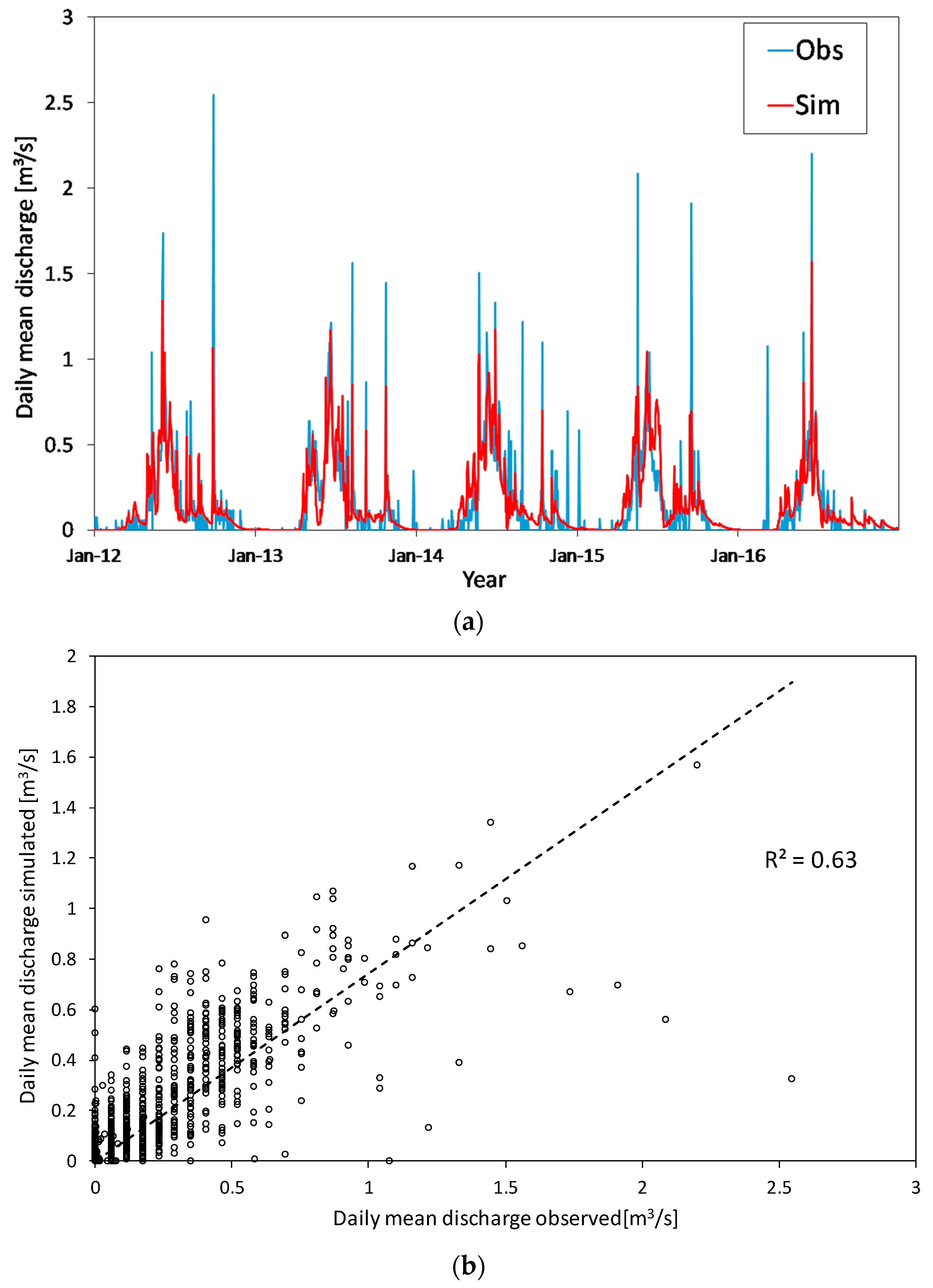
The hydrological model was calibrated based on 2012 observed data and validated with data of the period 2013–2016. Figure 2 compares and correlates the observed and simulated discharge for all the years of analysis. We also computed three indices to quantify the accuracy of the model: the volumetric deviation (ΔV), The Nash-Sutcliffe efficiency (NSE) and the Root Mean Square Error (RMSE). The value of volumetric deviation (ΔV) shows an overestimation of 2%. The NSE is equal to 0.68 [75,76] and the RMSE is 0.14 m3/s, indicating an accurate approximation. We also calculated the NSE value for the different seasons. It is 0.59 in spring, 0.75 in summer, 0.58 in autumn, and 0.80 in winter. Due to the absence of glacier coverage in the study catchment, the contribution of ice melt, i.e., the glacier mass balance, is neglected from the hydrological model.
The model captures the peaks in all years except for the years 2014 and 2015. This might be due to the low altitude and geographical position (in another catchment) of the weather station [60]. The Alps display a high spatial variability of precipitation; therefore, the station can underestimate or unrecord some events [72]. The snow melting computation also neglects factors like solar radiation [77], which could slightly affect the results. Future improvements of the hydrological model should include a more accurate description of this phenomenon. Nevertheless, the monthly values remain accurate (NSE > 0.9, RMSE ~ 0.05 m3/s), due to the small scale of the variability of the phenomena [78]. In the case of storage hydropower, we can expect that the misrepresentation of peaks will not affect the results, as they can be managed by the reservoir.
Table 3 provides the parameters obtained with the calibration and validation. The value of the runoff time parameter (kliq) is low because the catchment is very small. We also assumed that the time parameter of snow (ksnow) is 300 times kliq, because no studies were available. This conversion is based on the fact that the saturated snow conductivity is between 0.003–0.3 m/s [79], which is 9–900 times lower than the average velocity of a flood wave in the hydrographic network. The log parameter of sub/groundwater response (kbase) [26,80] and the temperature lapse rate (TLR) [60] come from the quoted literature. For further details, see Supplementary Material S1.
3.2. Validation of the Management Model
A heuristic optimization model must find the right balance between getting closer to the general optimum and limiting computational burden. The steps to calibrate the management model are described in the Supplementary Material S1. The model was validated as it provides revenue as high as the historical one. It can even outperform these results because we assumed “perfect foresight” conditions, which means inflows and electricity prices are known in advance. This represents an advantage for the model compared to historical management. Therefore, the curves on Figure 3 do not fit perfectly. However, this figure highlights that the model accurately simulates the actual management of the reservoir.
4. Future Scenarios: Results and Discussions
4.1. Climate Change Effects on Flow Regimes
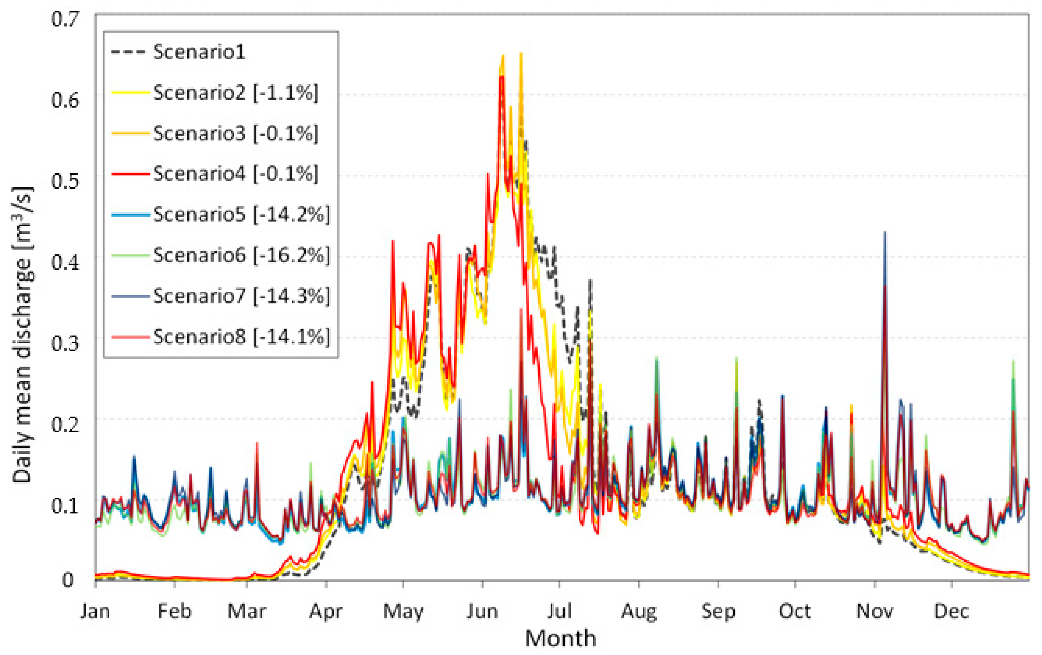
We simulated 100 synthetic time series of discharge for the period 2017–2046. We extracted the 95% confidence intervals for discharge for 2020, 2025, 2030 and 2045 to show the changes over time. Figure 4 shows the average daily discharge and the respective annual volumes for the year 2030. For detailed results, see Supplementary Material S1.
The discharge shows the typical behavior of snow-dominated catchments, characterized by seasonality in the runoff. Discharge is very low in winter due to cold temperatures and mainly solid precipitation. At the beginning of March, the temperatures rise, snow starts to melt, and runoff increases. From October, discharge decreases again because of falling temperatures. There is an offset between the period of the year in which snow falls on the ground and when it becomes liquid. The features listed above are well represented by the future-like-present scenario (climate scenario 1) in Figure 4. We can, therefore, guess the impact of temperature increases and precipitation evolutions on the seasonal availability of water. Figure 4 shows the effects induced by all eight climate change scenarios on discharge in terms of seasonality and cumulated volumes. The warmer-future scenarios (climate scenarios 2–4) exhibit an anticipation in spring peaks. The increase in the temperature would progressively anticipate seasonal snow ablation peaks, in turn affecting the shape of the discharge regime. In contrast, the annual volume of water does not change much, as precipitation does not evolve. The impact in this scenario remains limited because the catchment has no glaciers, which are very sensitive to climate change [26]. Here, only snowpack is impacted, reducing the effects of such scenarios. Comparing the results of discharge for warmer-future scenarios at 2030 with 2045, we observe lower values for the peaks and unlike in 2030, a drop of 11.5% in the daily mean discharge for climate scenario 4 is observed (for further information see Supplementary Material S1).
In liquid-only precipitation scenarios (climate scenarios 5–8), all the runoff becomes immediately available, snow does not “store” water. The catchment shows an immediate response to every event of precipitation and the seasonality is lost, as seen in Figure 4. The liquid-only precipitation climate scenarios indicate a theoretical limit case for a snow-dominated catchment and emphasizes the role of the loss of seasonality on the hydrological cycle [35]. In addition, the absence of glaciers in the catchment leads to no substantial inter-differences between temperature scenarios. Finally, the annual volume of water dramatically decreases in these scenarios, already in 2030. This is linked to the fact that an increase in the amount of liquid precipitation means an increase in ETP rate. In addition, as Tremorgio is a mid-altitude basin, the average monthly temperatures used in the computation of ETP would be higher, making this a significant influence. Please note that if temperature increases and there is a reduction of snow cover, then vegetation will increase; as a result, the ETP will also increase, affecting the runoff.
4.2. Impact of Climate Change on the Hydropower Plant
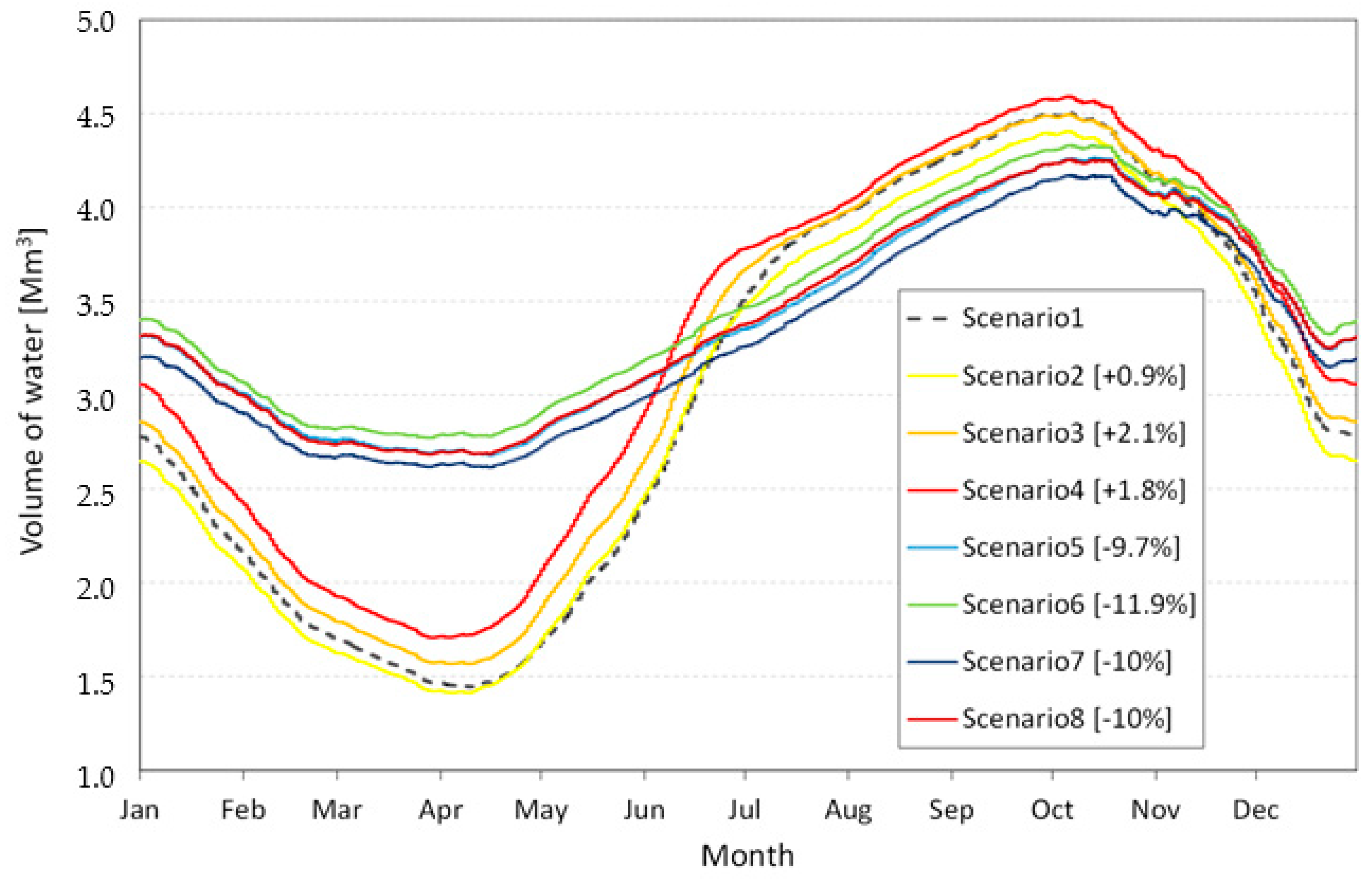
We ran the management model with the eight discharge scenarios in 2030 and the one in 2045 to assess the impact of climate changes on hydropower. We isolated this driver by only considering the historical electricity price. Figure 5 shows the average annual volumes of water in the reservoir for all the scenarios in 2030.
Warmer-future scenarios (i.e., climate scenarios 2–4) do not differ much from the base scenario. The curves are correlated, even if climate scenarios 3–4 anticipate the lowest level by 10 days. This pattern results from an anticipation of spring peaks, which means water can be emptied earlier. In addition, the increase in temperature lowly affects the annual volumes, the hydropower management, and in turn, the revenue. The 2030 base scenario’s income oscillates on the order of 1–2% (Figure 5). Liquid-only precipitation scenarios (i.e., climate scenarios 5–8), will tend to align water and price seasonality. Currently, in a Swiss snow-dominated catchment, the availability of water and the prices are out of phase. Runoff is scared in winter when prices peak and abundant in summer when prices drop. For optimal management, dam operators fill the reservoir in summer and empty it in winter. In the liquid-only precipitation scenarios, the offset between the two peaks diminishes. The increased runoff in winter can be immediately used, rather than being stored for generating during another price peak season. Less water is available in summer and must be transferred in winter. Under these climate conditions and for the purposes of maximizing revenue from hydropower production, the reservoir becomes oversized.
Please note that it is optimal to manage at the top, i.e., trying to reach the upper level of the lake at least once a year. A management at the bottom of the reservoir would not benefit from the hydraulic head effect [25]. A lower level means less energy generated by the amount of water, and in turn, lower revenue. This on-top management also appears in climate scenario 4 in 2045, where lesser runoff is expected. The relative reduction of revenue according to base scenario confirms the relevance of this strategy. It reduces losses, even at present, up to 10–12% in liquid-only precipitation scenarios and 8% for scenario 4 in 2045. Losses of revenue are present and cannot be avoided, but a proper management strategy can mitigate the impact of climate change, guaranteeing an improvement of 3% and about 4% in terms of energy and revenue losses, respectively.
4.3. Impacts of Electricity Price Scenarios
We do not present the impact of the twenty-eight spot electricity market scenarios on the reservoir volumes management, because it is marginal. We focus on the impact on incomes in 2030. Figure 6 shows the boxplot of the incomes of each price scenario, normalized with respect to the observed income of 2015.
The results are aligned with those found by Schillinger et al. [36], and differ slightly in the percentages of variation of median normalized income. Most price scenarios show an increase in income. In fact, only the deployment of renewable energy (R+, R−) represents a threat to hydropower. However, the increase in fuel or carbon prices can compensate for this loss of revenue. The worst price scenario (R+), i.e., a wind and solar increase of 10% more compared to EU reference scenario, exhibits a drop of 12% in the incomes. As shown by the German experience, an injection of photovoltaic (PV) and wind energy into the market provokes a rightward shift of the electricity supply curve and consequently a fall in spot prices [12]. In contrast, price scenario C++F++R− (a fast increase of carbon and fuel prices, a weak increase of wind and solar) generates an increase of 71% in hydropower incomes. If the EU trend is followed, the income will increase by 41%, thanks to a strong increase in fuel and carbon prices [70].
4.4. Mixed Scenarios
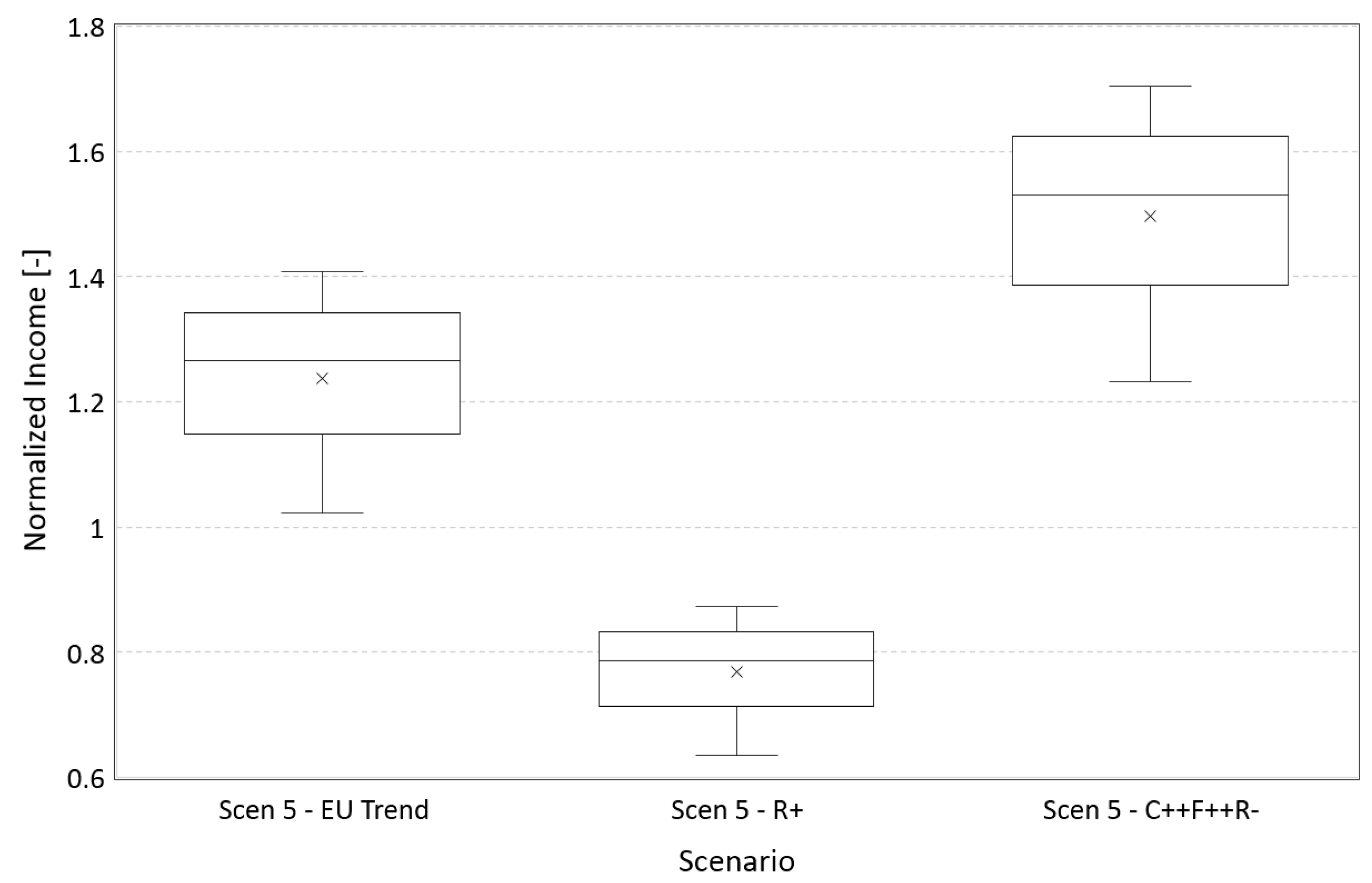
The mixed scenarios were built by combining one scenario from the climatic and three scenarios from the economic and computing the normalized incomes with respect to 2015. The liquid-precipitation future (climate scenario 5) was selected because the effects on volumes and incomes were the most significant. Water volumes and incomes decrease by 9.7% and 10%, respectively. The economic scenarios modelled consider the evolution of prices according to reference EU-Trend (+40% with respect to 2015 income), the so-called R+ scenario, which presents the highest income lost (−14% with respect to 2015 income), and the C++F++R− scenario, which conversely presents the highest increase (+70% with respect to 2015 income). We selected a few representative scenarios for the sake of clarity. Considering too many would not add much relevant information in terms of fundamental dynamics, as the reservoir can manage seasonality. It may have been more critical for a run-of-river installation.
The results in Figure 7 outline how the reduction of incoming volumes is balanced by the increase in prices implemented in the EU-Trend and C++F++R− scenarios, as the relative income increases in both cases (+24% and +50% respectively). On the other hand, the combination of economic and climatic scenarios that together implement a reduction in water volume and income causes the greatest reduction in normalized income at −23%. The main uncertainty for hydropower revenue comes from the electricity price. In contrast, for security of supply issues, climate change matters, as we see a significant drop of electricity generation, although this can be mitigated by smart management.
These considerations are obviously site-specific, linked to the hydrology and climatology of the area considered. The climate scenarios implemented are simple and, especially the liquid-only precipitation climate scenarios, are not suitable for short-term analysis, but could be a good theoretical comparison for long-term climate projections, especially for snow-dominated catchments. However, the losses in terms of electricity generation are aligned to studies present in existent literature for western Europe [31]. In addition, it was demonstrated the capability of the hydrological model to simulate with good accuracy in other catchments in the northern side of Alpine arch, while previously its performances had only been assessed on the Italian side [26,35].
5. Conclusions
This study assessed the future perspectives of hydropower in the challenging energetic Swiss framework through a case study in Leventina District, Canton Ticino. We considered the main drivers: climate change, renewable deployment, carbon and fuel prices. Climate change was modelled through a set of eight scenarios, implementing increasing trends in temperature and modification of the precipitation regime. A semi-distributed hydrological model was used to obtain future inflows. We investigated the impact of other drivers on hydropower according to twenty-eight electricity market scenarios. We simulated the impact on hydropower incomes thanks to a management model [25], which we modified. Climate change is likely to reduce the volume of water available for hydropower production and anticipate spring peaks in the discharge regime. We show that more water in winter and less in summer is expected in this catchment, as predicted in many other Alpine catchments in southern Switzerland. However, an optimal hydropower turbine schedule can mitigate these losses, including by benefiting from the maximum hydraulic head in managing at the top of the reservoir. Future market scenarios underline the antagonism between new renewable energies (wind and solar) deployment and hydropower revenue. The current market design undervalues the flexibility of hydropower (required to manage the intermittency of new renewable). Fortunately for hydropower operators, an increase in fuel and CO2 price can compensate for these losses, as observed in the ongoing European energy market. However, uncertainties involved in the study should not be overlooked, as problems are complex and many factors play an important role. There is obviously room for further investigations, including other case studies and comparing the analysis of these models on different types of hydropower plants (storage, run-of-the-river, and pumped-storage). There is a greater need to study the role of and factors influencing hydropower in the long term, due to the recent development and deployment of new and advanced energy storage technologies in the electricity grid.
Supplementary Materials
The following are available online at https://www.mdpi.com/2073-4441/10/9/1197/s1, Figure S1: Comparison of observed and simulated daily discharge of the year (a) 2012; (b) 2013; (c) 2014; (d) 2015; (e) 2016, Figure S2: Comparison of observed and simulated daily cumulated volumes of the year (a) 2012; (b) 2013; (c) 2014; (d) 2015; (e) 2016, Figure S3: Comparison of observed and simulated monthly discharge of the year (a) 2012; (b) 2013; (c) 2014; (d) 2015; (e) 2016, Figure S4: Comparison of the results obtained in terms of income with the four performances analysed, considering a progressively increasing number of steps. The results are normalized over the value obtained for the 2012, Figure S5: Comparison of the annual volumes simulated with the optimal configuration of parameters and the observed ones. Differences can be found due to the “perfect foresight” condition, Figure S6: Electricity spot prices for Switzerland in 2012, according to http://www.epexspot.com/, Figure S7: The behaviour of annual volumes for 2013 with the two values of maximum volume, where red is the maximum capacity of the reservoir, while orange is the maximum value observed from the real data available, Figure S8: Behaviour of annual volumes for 2014 with the two values of maximum volume, where red is the maximum capacity of the reservoir, while orange is the maximum value observed from the real data available, Figure S9: Behaviour of annual volumes for 2015 with the two values of maximum volume, where red is the maximum capacity of the reservoir, while orange is the maximum value observed from the real data, Figure S10: Average daily discharge for all the scenarios at (a) 2020; (b) 2025, Figure S11: Average daily discharge of all the scenarios at 2045, Figure S12: Cumulated volumes of all the scenarios, for the considered period of simulation, Figure S13: Comparison of hourly reservoir’s volumes for scenario 4 at 2030 and 2045, in terms of the average values with a 95% confidence interval, Figure S14: Comparison of hourly reservoir’s volumes for scenario 4 with different maximum volume, at 2045, in terms of the average values with a 95% confidence interval, Figure S15: Box plots comparison for scenario 4 with different V max at 2045. They are normalized with respect to base scenario, Table S1: Performance of the model in reproducing the observed discharge at reservoir outlet section. The analysis is made at daily and at monthly scale and is provided in terms of three performance indexes, RMSE (m3/s), NSE (-) and ΔV (-). Where Qobs and Vobs is the observed discharge and volume respectively, while Qsim and Vsim is the simulated discharge and volume respectively, Table S2: The behaviour of the different combinations. The steps needed to reach the observed income, and the income normalized over the observed income for 2012 at the highest number of steps is reported, Table S3: Normalized income over the observed income for the different simulations with increasing number of restarts, Table S4: Difference between the income found in the different simulations and the one found with only 1 restart, normalized over it. It allows to monitor the improvement in the objective function gained by increasing the restarts, Table S5: Overall results from calibration and validation years according to combination 4. The observed income for each step is reported along with the average of percentages found for validation years, Table S6: Annual volumes of all scenarios at 2045 for Tremorgio, along with the variation in volumes with respect to the base scenario i.e., scenario 1, Table S7: Variation income of all scenarios with respect to base scenario (2015). The results are arranged in descending order.
Author Contributions
Conceptualization, C.D.M.; Methodology, L.G.; Software, A.R., M.B., E.R.P. and L.G.; Validation, E.R.P. and L.G.; Formal Analysis, A.R. and M.B.; Investigation, A.R., M.B. and E.R.P.; Writing-Original Draft Preparation, A.R. and M.B.; Writing-Review & Editing, E.R.P., L.G. and C.D.M.; Visualization, E.R.P.; Supervision, L.G. and C.D.M.
Funding
This research received no external funding.
Acknowledgments
The authors would like to thank AET, the company that manages the Tremorgio reservoir, for providing measured hydrological data at Tremorgio, and MeteoSwiss for providing meteorological data. The electricity price data were collected from EPEX SPOT SE. The research is part of the cluster project ‘The Future of Swiss Hydropower: An Integrated Economic Assessment of Chances, Threats and Solutions’ (HP Future) that is undertaken within the frame of the National Research Programme 70 ‘Energy Turnaround’ (www.nrp70.ch) of the Swiss National Science Foundation. The data used are also listed in the references and the Supplementary Material S1. We acknowledge the constructive suggestions by the two anonymous reviewers that greatly improved the paper.
Conflicts of Interest
The authors declare no conflict of interest.
References
- Apadula, F.; Bassini, A.; Elli, A.; Scapin, S. Relationships between meteorological variables and monthly electricity demand. Appl. Energy 2012, 98, 346–356. [Google Scholar] [CrossRef]
- Swiss Federal Council Message Relatif Au Premier Paquet De Mesures De La Stratégie Enérgétique 2050. Available online: www.news.admin.ch/message/index.html?lang=fr&msg-id=50123 (accessed on 4 March 2018).
- International Renewable Energy Agency (IRENA). Global Energy Transformation: A Roadmap to 2050; IRENA: Abu Dhabi, the United Arab Emirates, 2018. [Google Scholar]
- IEA. Energy and Climate Change; World Energy Outlook Special Report; IEA: Paris, France, 2015. [Google Scholar]
- Cherp, A.; Vinichenko, V.; Jewell, J.; Suzuki, M.; Antal, M. Comparing electricity transitions: A historical analysis of nuclear, wind and solar power in Germany and Japan. Energy Policy 2017, 101, 612–628. [Google Scholar] [CrossRef] [Green Version]
- Valentine, S.V. Japanese wind energy development policy: Grand plan or group think? Energy Policy 2011, 39, 6842–6854. [Google Scholar] [CrossRef]
- Glaser, A. From Brokdorf to Fukushima: The long journey to nuclear phase-out. Bull. At. Sci. 2012, 68, 10–21. [Google Scholar] [CrossRef]
- Feldhoff, T. Post-Fukushima energy paths: Japan and Germany compared. Bull. At. Sci. 2014, 70, 87–96. [Google Scholar] [CrossRef]
- Jones, L.E. Renewable Energy Integration: Practical Management of Variability, Uncertainty and Flexibility in Power Grids, 1st ed.; Elsevier Inc.: New York, NY, USA, 2014; ISBN 9780124079106. [Google Scholar]
- Verzijlbergh, R.A.; De Vries, L.J.; Dijkema, G.P.J.; Herder, P.M. Institutional challenges caused by the integration of renewable energy sources in the European electricity sector. Renew. Sustain. Energy Rev. 2017, 75, 660–667. [Google Scholar] [CrossRef] [Green Version]
- Scherer, L.; Pfister, S. Hydropower’s Biogenic Carbon Footprint. PLoS ONE 2016, 11, e0161947. [Google Scholar] [CrossRef] [PubMed]
- Gaudard, L.; Romerio, F. The future of hydropower in Europe: Interconnecting climate, markets and policies. Environ. Sci. Policy 2014, 37, 172–181. [Google Scholar] [CrossRef]
- Ravazzani, G.; Dalla Valle, F.; Gaudard, L.; Mendlik, T.; Gobiet, A.; Mancini, M. Assessing Climate Impacts on Hydropower Production: The Case of the Toce River Basin. Climate 2016, 4, 16. [Google Scholar] [CrossRef] [Green Version]
- Stocker, T.F.; Qin, D.; Plattner, G.K.; Tignor, M.; Allen, S.K.; Boschung, J.; Nauels, A.; Xia, Y.; Bex, V.; Midgley, P.M. Climate Change 2013: The Physical Science Basis; IPCC: Cambridge, UK; New York, NY, USA, 2013. [Google Scholar]
- Brunetti, M.; Lentini, G.; Maugeri, M.; Nanni, T.; Auer, I.; Böhm, R.; Schöner, W. Climate variability and change in the greater alpine region over the last two centuries based on multi-variable analysis. Int. J. Climatol. 2009, 29, 2197–2225. [Google Scholar] [CrossRef]
- Brunetti, M.; Maugeri, M.; Nanni, T.; Auer, I.; Böhm, R.; Schöner, W. Precipitation variability and changes in the greater Alpine region over the 1800–2003 period. J. Geophys. Res. Atmos. 2006, 111. [Google Scholar] [CrossRef] [Green Version]
- Gobiet, A.; Kotlarski, S.; Beniston, M.; Heinrich, G.; Rajczak, J.; Stoffel, M. 21st century climate change in the European Alps—A review. Sci. Total Environ. 2014, 493, 1138–1151. [Google Scholar] [CrossRef] [PubMed]
- Lehner, B.; Czisch, G.; Vassolo, S. The impact of global change on the hydropower potential of Europe: A model-based analysis. Energy Policy 2005, 33, 839–855. [Google Scholar] [CrossRef]
- Wagner, T.; Themeßl, M.; Schüppel, A.; Gobiet, A.; Stigler, H.; Birk, S. Impacts of climate change on stream flow and hydro power generation in the Alpine region. Environ. Earth Sci. 2017, 76, 4. [Google Scholar] [CrossRef]
- Schaefli, B.; Hingray, B.; Musy, A. Climate change and hydropower production in the Swiss Alps: Quantification of potential impacts and related modelling uncertainties. Hydrol. Earth Syst. Sci. 2007, 11, 1191–1205. [Google Scholar] [CrossRef]
- Koch, F.; Prasch, M.; Bach, H.; Mauser, W.; Appel, F.; Weber, M. How will hydroelectric power generation develop under climate change scenarios? A case study in the upper Danube basin. Energies 2011, 4, 1508–1541. [Google Scholar] [CrossRef] [Green Version]
- Majone, B.; Villa, F.; Deidda, R.; Bellin, A. Impact of climate change and water use policies on hydropower potential in the south-eastern Alpine region. Sci. Total Environ. 2016, 543, 965–980. [Google Scholar] [CrossRef] [PubMed]
- Schaefli, B. Projecting hydropower production under future climates: A guide for decision-makers and modelers to interpret and design climate change impact assessments. Wiley Interdiscip. Rev. Water 2015, 2, 271–289. [Google Scholar] [CrossRef]
- Beniston, M. Impacts of climatic change on water and associated economic activities in the Swiss Alps. J. Hydrol. 2012, 412–413, 291–296. [Google Scholar] [CrossRef]
- Gaudard, L.; Gilli, M.; Romerio, F. Climate Change Impacts on Hydropower Management. Water Resour. Manag. 2013, 27, 5143–5156. [Google Scholar] [CrossRef]
- Bongio, M.; Avanzi, F.; De Michele, C. Hydroelectric power generation in an Alpine basin: Future water-energy scenarios in a run-of-the-river plant. Adv. Water Resour. 2016, 94, 318–331. [Google Scholar] [CrossRef]
- Finger, D.; Heinrich, G.; Gobiet, A.; Bauder, A. Projections of future water resources and their uncertainty in a glacierized catchment in the Swiss Alps and the subsequent effects on hydropower production during the 21st century. Water Resour. Res. 2012, 48. [Google Scholar] [CrossRef] [Green Version]
- Hänggi, P.; Weingartner, R. Variations in Discharge Volumes for Hydropower Generation in Switzerland. Water Resour. Manag. 2012, 26, 1231–1252. [Google Scholar] [CrossRef]
- Ahmed, T.; Muttaqi, K.M.; Agalgaonkar, A.P. Climate change impacts on electricity demand in the State of New South Wales, Australia. Appl. Energy 2012, 98, 376–383. [Google Scholar] [CrossRef]
- Christenson, M.; Manz, H.; Gyalistras, D. Climate warming impact on degree-days and building energy demand in Switzerland. Energy Convers. Manag. 2006, 47, 671–686. [Google Scholar] [CrossRef]
- Golombek, R.; Kittelsen, S.A.C.; Haddeland, I. Climate change: Impacts on electricity markets in Western Europe. Clim. Chang. 2012, 113, 357–370. [Google Scholar] [CrossRef] [PubMed]
- Maran, S.; Volonterio, M.; Gaudard, L. Climate change impacts on hydropower in an alpine catchment. Environ. Sci. Policy 2014, 43, 15–25. [Google Scholar] [CrossRef]
- Madani, K.; Guégan, M.; Uvo, C.B. Climate change impacts on high-elevation hydroelectricity in California. J. Hydrol. 2014, 510, 153–163. [Google Scholar] [CrossRef]
- Guegan, M.; Madani, K.; Uvo, C.B. Climate Change Effects on the High Elevation Hydropower System with Consideration of Warming Impacts on Electricity Demand and Pricing; California Energy Commission: Sacramento, CA, USA, 2012.
- Gaudard, L.; Avanzi, F.; De Michele, C. Seasonal aspects of the energy-water nexus: The case of a run-of-the-river hydropower plant. Appl. Energy 2018, 210, 604–612. [Google Scholar] [CrossRef]
- Schillinger, M.; Weigt, H.; Barry, M.; Schumann, R. Hydropower Operation in a Changing Market Environment—A Swiss Case Study. SSRN Electron. J. 2017. [Google Scholar] [CrossRef]
- Winemiller, K.O.; McIntyre, P.B.; Castello, L.; Fluet-Chouinard, E.; Giarrizzo, T.; Nam, S.; Baird, I.G.; Darwall, W.; Lujan, N.K.; Harrison, I.; et al. Balancing hydropower and biodiversity in the Amazon, Congo, and Mekong. Science 2016, 351, 128–129. [Google Scholar] [CrossRef] [PubMed] [Green Version]
- Ziv, G.; Baran, E.; Nam, S.; Rodríguez-Iturbe, I.; Levin, S.A. Trading-off fish biodiversity, food security, and hydropower in the Mekong River Basin. Proc. Natl. Acad. Sci. USA 2012, 109, 5609–5614. [Google Scholar] [CrossRef] [PubMed] [Green Version]
- Poff, N.L.; Olden, J.D. Can dams be designed for sustainability? Science 2017, 358, 1252–1253. [Google Scholar] [CrossRef] [PubMed]
- Liao, X.; Zhou, J.; Ouyang, S.; Zhang, R.; Zhang, Y. Multi-objective artificial bee colony algorithm for long-term scheduling of hydropower system: A case study of China. Water Util. J. 2014, 7, 13–23. [Google Scholar]
- Kougias, I.; Katsifarakis, L.; Theodossiou, N. Medley Multiobjective Harmony Search Algorithm: Application on a water resources management problem. Eur. Water 2012, 39, 41–52. [Google Scholar]
- Afshar, A.; Shafii, M.; Haddad, O.B. Optimizing multi-reservoir operation rules: An improved HBMO approach. J. Hydroinform. 2010, 13, 121–139. [Google Scholar] [CrossRef]
- Ahmadi, M.; Bozorg Haddad, O.; Mariño, M.A. Extraction of Flexible Multi-Objective Real-Time Reservoir Operation Rules. Water Resour. Manag. 2014, 28, 131–147. [Google Scholar] [CrossRef]
- Haddad, O.B.; Afshar, A.; Mariño, M.A. Honey-bees mating optimization (HBMO) algorithm: A new heuristic approach for water resources optimization. Water Resour. Manag. 2006, 20, 661–680. [Google Scholar] [CrossRef]
- Wagner, B.; Hauer, C.; Schoder, A.; Habersack, H. A review of hydropower in Austria: Past, present and future development. Renew. Sustain. Energy Rev. 2015, 50, 304–314. [Google Scholar] [CrossRef]
- Cherry, J.E.; Knapp, C.; Trainor, S.; Ray, A.J.; Tedesche, M.; Walker, S. Planning for climate change impacts on hydropower in the Far North. Hydrol. Earth Syst. Sci. 2017, 21, 133–151. [Google Scholar] [CrossRef] [Green Version]
- Bliss, A.; Hock, R.; Radić, V. Global response of glacier runoff to twenty-first century climate change. J. Geophys. Res. Earth Surf. 2014, 119, 717–730. [Google Scholar] [CrossRef] [Green Version]
- Gaudard, L.; Gabbi, J.; Bauder, A.; Romerio, F. Long-term Uncertainty of Hydropower Revenue Due to Climate Change and Electricity Prices. Water Resour. Manag. 2016, 30, 1325–1343. [Google Scholar] [CrossRef] [Green Version]
- Swiss Federal Office of Energy (SFOE). Swiss Statistics of Electricity 2017. Available online: http://www.bfe.admin.ch/themen/00526/00541/00542/00630/index.html?lang=en&dossier_id=00765 (accessed on 4 March 2018).
- Glomsrød, S.; Wei, T.; Mideksa, T.; Samset, B.H. Energy market impacts of nuclear power phase-out policies. Mitigation Adaptation Strateg. Glob. Change 2015, 20, 1511–1527. [Google Scholar] [CrossRef]
- Redondo, P.D.; van Vliet, O. Modelling the Energy Future of Switzerland after the Phase Out of Nuclear Power Plants. Energy Procedia 2015, 76, 49–58. [Google Scholar] [CrossRef]
- Gaudard, L.; Romerio, F.; Dalla Valle, F.; Gorret, R.; Maran, S.; Ravazzani, G.; Stoffel, M.; Volonterio, M. Climate change impacts on hydropower in the Swiss and Italian Alps. Sci. Total Environ. 2014, 493, 1211–1221. [Google Scholar] [CrossRef] [PubMed]
- Bartolini, E.; Allamano, P.; Laio, F.; Claps, P. Runoff regime estimation at high-elevation sites: A parsimonious water balance approach. Hydrol. Earth Syst. Sci. 2011, 15, 1661–1673. [Google Scholar] [CrossRef]
- Thornthwaite, C.W. An Approach toward a Rational Classification of Climate. Geogr. Rev. 1948, 38, 55–94. [Google Scholar] [CrossRef]
- Rango, A.; Martinec, J. Revisiting the degree-day method for snowmelt computations. JAWRA J. Am. Water Resour. Assoc. 1995, 31, 657–669. [Google Scholar] [CrossRef]
- Mockus Victor Design Hydrographs. National Engineering Handbook; U.S. Department of Agriculture: Washington, DC, USA, 1972; p. 127.
- Bahr, D.; Meier, M.; Peckham, S. The physical basis of volume-area scaling. J. Geophys. Res. 1997, 102, 20335–20362. [Google Scholar] [CrossRef]
- Nash, J.E. The form of the instantaneous unit hydrograph. Int. Assoc. Hydrol. Sci. 1957, 45, 114–121. [Google Scholar]
- Avanzi, F.; De Michele, C.; Ghezzi, A.; Jommi, C.; Pepe, M. A processing-modeling routine to use SNOTEL hourly data in snowpack dynamic models. Adv. Water Resour. 2014, 73, 16–29. [Google Scholar] [CrossRef]
- Rolland, C. Spatial and seasonal variations of air temperature lapse rates in alpine regions. J. Clim. 2003, 16, 1032–1046. [Google Scholar] [CrossRef]
- Nash, J.E.; Sutcliffe, J.V. River flow forecasting through conceptual models part I—A discussion of principles. J. Hydrol. 1970, 10, 282–290. [Google Scholar] [CrossRef]
- DeWalle, D.R.; Rango, A. Principles of Snow Hydrology; Cambridge University Press: Cambridge, UK, 2008; ISBN 9780511535673. [Google Scholar]
- Dueck, G.; Scheuer, T. Threshold accepting: A general purpose optimization algorithm appearing superior to simulated annealing. J. Comput. Phys. 1990, 90, 161–175. [Google Scholar] [CrossRef]
- Moscato, P.; Fontanari, J.F. Stochastic versus deterministic update in simulated annealing. Phys. Lett. A 1990, 146, 204–208. [Google Scholar] [CrossRef]
- Winker, P. Optimization Heuristics in Econometrics: Application of Threshold Accepting; Wiley: Hoboken, NJ, USA, 2001; ISBN 978-0-471-85631-3. [Google Scholar]
- Kottegoda, N.T.; Rosso, R. Applied Statistics for Civil and Environmental Engineers; Wiley-Blackwell: Oxford, UK, 2008; ISBN 978-1-405-17917-1. [Google Scholar]
- Beniston, M. Mountain climates and climatic change: An overview of processes focusing on the European Alps. Pure Appl. Geophys. 2005, 162, 1587–1606. [Google Scholar] [CrossRef]
- Böhm, R.; Auer, I.; Brunetti, M.; Maugeri, M.; Nanni, T.; Schöner, W. Regional temperature variability in the European Alps: 1760–1998 from homogenized instrumental time series. Int. J. Clim. 2001, 21, 1779–1801. [Google Scholar] [CrossRef]
- Cislaghi, M.; De Michele, C.; Ghezzi, A.; Rosso, R. Statistical assessment of trends and oscillations in rainfall dynamics: Analysis of long daily Italian series. Atmos. Res. 2005, 77, 188–202. [Google Scholar] [CrossRef]
- European Comission. EU Reference Scenario. 2016. Available online: https://ec.europa.eu/energy/sites/ener/files/documents/ref2016_report_final-web.pdf (accessed on 20 March 2018).
- AET Impianto idroelettrico Tremorgio. Available online: https://www.aet.ch/IT/Impianto-idroelettrico-Tremorgio-e68a9800#.Wq62d_nwbct (accessed on 18 March 2018).
- Krajewski, W.F.; Ciach, G.J.; Habib, E. An analysis of small-scale rainfall variability in different climatic regimes. Hydrol. Sci. J. 2003, 48, 151–162. [Google Scholar] [CrossRef] [Green Version]
- WSL CORINE Switzerland. Available online: https://www.wsl.ch/en/projects/corine-switzerland.html (accessed on 20 March 2018).
- MeteoSchweiz. Rapporto Sul Clima—Cantone Ticino. 2012. Available online: https://www.meteoschweiz.admin.ch/home/service-und-publikationen/publikationen.subpage.html/de/data/publications/2012/1/rapporto-sul-clima---cantone-ticino.html (accessed on 20 March 2018).
- Cheng, K.S.; Lien, Y.T.; Wu, Y.C.; Su, Y.F. On the criteria of model performance evaluation for real-time flood forecasting. Stoch. Environ. Res. Risk Assess. 2017, 31, 1123–1146. [Google Scholar] [CrossRef]
- Moriasi, D.N.; Arnold, J.G.; Van Liew, M.W.; Bingner, R.L.; Harmel, R.D.; Veith, T.L. Model Evaluation Guidelines For Systematic Quantification Of Accuracy in Watershed Simulations. Am. Soc. Agric. Biol. Eng. 2007, 50, 885–900. [Google Scholar]
- Hock, R. Temperature index melt modelling in mountain areas. J. Hydrol. 2003, 282, 104–115. [Google Scholar] [CrossRef] [Green Version]
- Wang, Q.J.; Pagano, T.C.; Zhou, S.L.; Hapuarachchi, H.A.P.; Zhang, L.; Robertson, D.E. Monthly versus daily water balance models in simulating monthly runoff. J. Hydrol. 2011, 404, 166–175. [Google Scholar] [CrossRef]
- Katsushima, T.; Yamaguchi, S.; Kumakura, T.; Sato, A. Experimental analysis of preferential flow in dry snowpack. Cold Reg. Sci. Technol. 2013, 85, 206–216. [Google Scholar] [CrossRef]
- Eng, K.; Milly, P.C.D. Relating low-flow characteristics to the base flow recession time constant at partial record stream gauges. Water Resour. Res. 2007, 43. [Google Scholar] [CrossRef] [Green Version]
Figure 1.
Schematic representation of the hydropower management model, after Gaudard et al. [25].
Figure 1.
Schematic representation of the hydropower management model, after Gaudard et al. [25].

Figure 2.
Time series plot (a) and comparison (b) between the simulated and observed discharge for 2012–2016. R2 is the correlation coefficient.
Figure 2.
Time series plot (a) and comparison (b) between the simulated and observed discharge for 2012–2016. R2 is the correlation coefficient.

Figure 3.
Comparison of the actual and simulated reservoir volumes for Tremorgio (1 January 2012 to 31 December 2012).
Figure 3.
Comparison of the actual and simulated reservoir volumes for Tremorgio (1 January 2012 to 31 December 2012).

Figure 4.
Daily discharge in Tremorgio reservoir for all climate scenarios modelled in 2030. They represent average values obtained from a 95% confidence interval. The mean annual volume variation relative to scenario 1 is shown for all scenarios.
Figure 4.
Daily discharge in Tremorgio reservoir for all climate scenarios modelled in 2030. They represent average values obtained from a 95% confidence interval. The mean annual volume variation relative to scenario 1 is shown for all scenarios.

Figure 5.
Evolution of the reservoir’s volumes in 2030 for all climate scenarios, with a 95% confidence interval. The mean income variation relative to scenario 1 is shown for all scenarios.
Figure 5.
Evolution of the reservoir’s volumes in 2030 for all climate scenarios, with a 95% confidence interval. The mean income variation relative to scenario 1 is shown for all scenarios.

Figure 6.
Boxplots of normalized incomes (according to 2015) for all price scenarios in 2030.

Figure 7.
Boxplots of normalized incomes (according to 2015) for 2030 mixed scenarios.


Table 1.
Price scenarios used in this work, according to [36].
Table 1.
Price scenarios used in this work, according to [36].
| Scenario | Explanation |
|---|---|
| EU Reference Scenario (Scenario 1) | As in EU Energy Trends 1 |
| Base Price 2015 Scenario (Scenario 2) | Carbon or fuel prices supposed to be equal to 2015 |
| C+ (Scenario 3) | Slow increase of carbon price (35 €/t in 2030) |
| C++ (Scenario 4) | Fast increase in carbon price (50 €/t in 2030) |
| F+ (Scenario 5) | Slow increase in fuel price (+50% until 2030) |
| F++ (Scenario 6) | Fast increase in fuel price (+100% until 2030) |
| R+ (Scenario 7) | Stronger increase in wind and solar (+10% relative to EU Trend) |
| R− (Scenario 8) | Weaker increase in wind and solar (−10% relative to EU Trend) |
| Combinations (Scenarios from 9 to 28) | Combination of all the scenarios |
1 EU reference scenario [70].
Table 2.
Main characteristics of the Tremorgio power plant, reservoir and catchment.
| Tremorgio Basin and Power Plant | |
|---|---|
| Catchment area (km2) | 5.07 |
| Glacier coverage (%) | 0 |
| Maximum elevation (m a.s.l.) | 2635 |
| Minimum elevation (m a.s.l.) | 1830 |
| Reservoir volume available (Mm3) | 5.54 |
| Maximum reservoir elevation (m a.s.l.) | 1830 |
| Minimum reservoir elevation (m a.s.l.) | 1800 |
| Power plant elevation (m a.s.l) | 950 |
| Maximum discharge (m3/s) | 1.6 |
| Type of turbine | Pelton |
| Power installed (MW) | 10 |
| Efficiency (-) | 0.75 |
Table 3.
Parameters after calibration and validation for Tremorgio basin. kliq is the runoff time parameter, ksnow is the time parameter of snow, kbase is the time parameter of groundwater, DDFmin is the minimum value of degree-day factor, DDFmax is the maximum value of degree-day factor, and TLR is the temperature lapse rate.
| n | kliq (days) | ksnow (days) | kbase (days) | DDFmin (mm/d°C) | DDFmax (mm/d°C) | TLR (°C/100 m) |
|---|---|---|---|---|---|---|
| 3.5 | 0.06 | 18 | 14 | 1.05 | 3.35 | 0.58 |
© 2018 by the authors. Licensee MDPI, Basel, Switzerland. This article is an open access article distributed under the terms and conditions of the Creative Commons Attribution (CC BY) license (http://creativecommons.org/licenses/by/4.0/).
Share and Cite
MDPI and ACS Style
Ranzani, A.; Bonato, M.; Patro, E.R.; Gaudard, L.; De Michele, C. Hydropower Future: Between Climate Change, Renewable Deployment, Carbon and Fuel Prices. Water 2018, 10, 1197. https://doi.org/10.3390/w10091197
AMA Style
Ranzani A, Bonato M, Patro ER, Gaudard L, De Michele C. Hydropower Future: Between Climate Change, Renewable Deployment, Carbon and Fuel Prices. Water. 2018; 10(9):1197. https://doi.org/10.3390/w10091197
Chicago/Turabian StyleRanzani, Alessandro, Mattia Bonato, Epari Ritesh Patro, Ludovic Gaudard, and Carlo De Michele. 2018. "Hydropower Future: Between Climate Change, Renewable Deployment, Carbon and Fuel Prices" Water 10, no. 9: 1197. https://doi.org/10.3390/w10091197
Note that from the first issue of 2016, this journal uses article numbers instead of page numbers. See further details here.