Effect of a Lateral Jet on the Turbulent Flow Characteristics of an Open Channel Flow with Rigid Vegetation


1
State Key Laboratory of Eco-Hydraulic in Northwest Arid Region of China, Xi’an University of Technology, Xi’an 710048, China
2
State Key Laboratory of Simulation and Regulation of Water Cycle in River Basin, China Institute of Water Resources and Hydropower Research, Beijing 100038, China
3
Department of Water Environment, China Institute of Water Resources and Hydropower Research, Beijing 100038, China
4
Department of River Engineering, Wuhan University, Wuhan 430072, China
*
Author to whom correspondence should be addressed.
Water 2018, 10(9), 1204; https://doi.org/10.3390/w10091204
Submission received: 2 August 2018
/
Revised: 26 August 2018
/
Accepted: 3 September 2018
/
Published: 6 September 2018
(This article belongs to the Section Water Quality and Contamination)
Abstract
:Aquatic vegetation can purify polluted bodies of water and beautify the environment, as well as alter the structure of water flow and affect the migration and diffusion of pollutants in bodies of water. Vegetation can significantly change the original water flow, especially in cases in which aquatic vegetation interacts with a jet. Characteristics of jet flow open channels without vegetation have been studied, but research on the characteristics of open-channel flows under the action of lateral jets and in the presence of vegetation are rare. High-frequency particle image velocimetry (PIV) was used to measure a lateral jet in water with rigid vegetation and our results were compared to the lateral jet flow field in water without vegetation. The results show that the vegetation arrangement and vegetation resistance cause significant changes. The presence of vegetation increased the surface velocity of the water, and the flow velocity decreased in the interior area of the vegetation and near the bottom of the water tank. The changes in flow velocity with changes in water depth displayed “S” type and anti-“S” type distributions, and the flow velocity of free layer was approximately logarithmic. Due to vegetation resistance and jet pressure differences, the lateral jet trajectory in water with vegetation was more likely to bend than in water without vegetation. The turbulence intensity and Reynolds stress had different distributions for water with and without vegetation. At the top of the vegetation and near the water surface, turbulent mixing of the water flow was strong, the flow velocity gradient was large and the turbulence intensity and the Reynolds stress reached their maxima. The effects of a lateral jet on an open-channel flow were compared for different vegetation conditions, revealing that a rhombic vegetation arrangement has a stronger deceleration effect than other arrangements. The theoretical results can be applied to wastewater discharge into vegetation channels.
1. Introduction
Maintaining healthy rivers and promoting the sustainable use of water resources are important issues faced by water resource managers and scientific researchers. Moreover, maintaining and restoring a river’s ecological environment is crucial for sustainable development. Aquatic plants in river courses have an important influence on a river’s ecosystem. Plants not only directly affect the transport of sediment, pollutants and nutrients in rivers, but they also affect the spread of pollutants and change the movement of bedloads and suspended sediments in rivers. Under the action of water flow, plants will bend and deform the flow and introduce flow fluctuations. Therefore, determining how to maximize the beneficial effects of aquatic vegetation in rivers while suppressing their adverse effects is vital for the ecological restoration of rivers and flood control.
Turbulent jets have been widely studied analytically, computationally, and experimentally for several decades in a wide range of fields, including water conservation and hydropower engineering, aerospace engineering, water supply and drainage engineering and environmental engineering [1,2,3,4,5,6,7,8,9]. In combination with environmental water conservation projects, turbulent jets play an important role in the discharge of effluents into water systems, including rivers, streams, lakes, seas and water in the atmosphere. The jet mixing process is strongly affected by the initial jet characteristics (such as nozzle shape, dimensions, submerged port height, and flow rate), boundary conditions (such as topography, bathymetry and physical properties) and the hydrodynamic features of the cross current (such as depth, flow rate, stratification and wave motion) [10,11,12,13]. Therefore, an understanding of the basic mixing mechanisms of jets could have significant importance for both the engineering control design and the environmental management monitoring sectors.
Turbulent jets play a fundamental and important role as the turbulent shear stream in crossflow. An understanding of the characteristics of jet flows is critical to solving a variety of industrial and environmental problems [2,11,14]. Lee [15], Zeng [16], Zhang T [17] and Li W [18] studied the jet axis velocity, the attenuation law of the concentration and the penetration height of the jet from an experimental point of view. Using trajectory equations, theoretical formulas of dilution along the path based on a numerical simulation (e.g., finite difference method and RNG k-ε turbulence), LES simulation and the turbulent integral model, Gao, M [19], Meftah et al. [20,21] simulated the effects of jets in crossflows, and their numerical simulation results were in good agreement with the experimental ones.
The effect of vegetation on flow is important for material exchange and energy transfer in river ecosystems. The use of natural vegetation for slope protection, soil purification, water quality improvement and river ecological environment has become an important factor for river ecological rehabilitation. Vegetation in channels strongly affects flow structure and turbulence, which has consequences for the hydrological storage of nutrients and chemical tracers, the shelter for stream biota and the trapping and transport of sediments. In recent years, many researchers have studied the structure of open-channel flow under the action of vegetation. Yang et al. [21] and Nepf et al. [22] considered flow laws in the presence of vegetation and experimentally analyzed the resistance of vegetation to flow for submerged and emergent plants. Zhang et al. [23] and Li et al. [24] demonstrated that a mathematical model could be used to simulate the influence of vegetation on flow. By using the resistance formula for flow around a cylinder, Huai et al. [25] calculated the water flow resistance around vegetation. Additionally, based on the research results of Li 1973 [26], Lindner et al. [27] derived a method for calculating a vegetation resistance coefficient Cd and proposed that the vegetation resistance factor is determined by the horizontal and vertical distance of vegetation and the diameter of the vegetation. For submerged vegetation, Murphy et al. [28] established a new longitudinal velocity distribution model in open-channel flows, and found the results predicted by the model to be consistent with experimental data. Serio et al. [29] studied the mechanism for transport and diffusion in open channels under the action of rigid vegetation and flexible vegetation. Their results showed that vegetation density and stiffness have different effects on the temporal and spatial distribution of time-average flow velocity in open channels.
The work described in Meftah et al. [30] and Ben Meftah et al. [20] showed that turbulent jets play an important role in the initial mixing phase for pollutants discharged into jets, such as wastewater discharged into streams. To explore different methods of jet discharge, Ben et al. [31] considered a bottom jet discharge into an open channel with vegetation and analyzed the influence of non-submerged rigid vegetation and a lateral jet on the open channel. The results showed that the jet penetration height within the ambient flow significantly changed the flow velocity field in the open channel. Similarly, Malcangio et al. [32] showed that rigid vegetation had a significant effect on the lateral circular orifice floating jet; it decreased the flow velocity in the crossflow and increased the penetration height and dilution of the jet significantly. Meftah et al. [33] observed vertical dense jets in a crossflow, flow field, jet trajectory, turbulence intensity, turbulent kinetic energy, turbulent length scale and diffusion coefficient with an emphasis on the higher turbulence intensity of the jet field and the higher turbulent energy. When there was no jet, the environmental flow field was isotropic. When there was a jet field, the environmental flow field was anisotropic and changed with the turbulence length scale.
Most studies focused on either the jet in a crossflow or on the vegetation in an open channel, but few have studied these two factors simultaneously. There has been even less study of the interaction between lateral jets and different vegetation arrangements. To study the interaction between a jet and vegetation, we studied the following under different vegetation conditions: (1) the variation of the average flow-field distribution of a lateral jet in an open channel; (2) the longitudinal jet flow velocity along a vertical line; (3) the trajectory of a transverse jet; and (4) the turbulence intensity and Reynolds stress. The flow mechanism under rigid vegetation was revealed by analyzing the flow velocity, transverse jet motion trajectory, turbulence intensity and Reynolds stress along a vertical line of transverse jet horizontal and longitudinal sections, and the influence of vegetation on the lateral jet under different working conditions was compared. It was found that a rhombic arrangement of vegetation had a stronger deceleration effect than other arrangements. The theoretical results can be applied to wastewater discharge problems in vegetation channels.
2. Experimental Equipment and Conditions
2.1. Sink Device
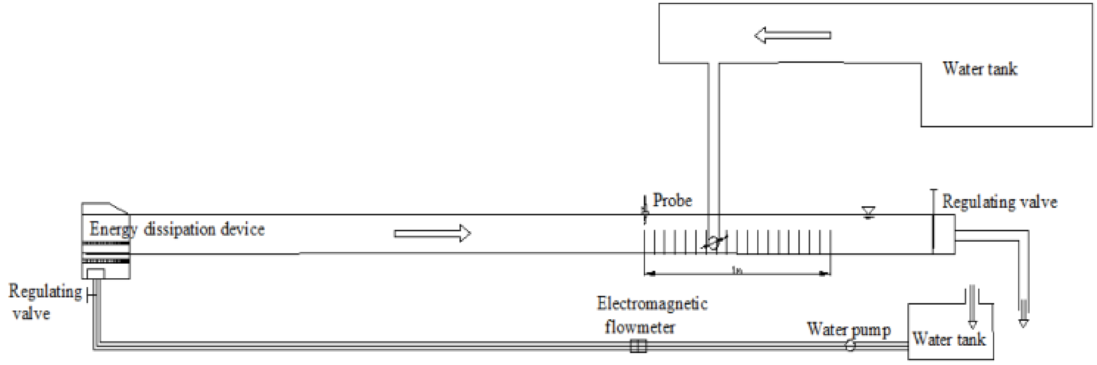
The experimental equipment consisted of a water supply device, a steady-flow device, a test water tank and a water return device (Figure 1). The experiments were conducted in the National Key Laboratory of Ecological and Water Conservancy of Northwest Arid Region of Xi’an University of Technology. The channel was constructed from plexiglass, and was 7.3 m long, 0.3 m wide and 0.25 m deep. In order to ensure the stability of the flow, a trash rack, a glass ball and a floating row were arranged at the head of the sink. The side row jet hole was set at a distance of 2.6 m from the inlet of the water tank. The diameter of the jet hole was 0.01 m, which was represented by D, and the hole was installed at a distance of 0.1 m from the bottom of the water tank. The center of the jet orifice was considered to be the origin of the coordinate system. The direction of the ambient flow velocity was set as the x axis, the vertical axis was the z axis and the direction of the jet was the y axis. A glass rotor flowmeter (Model LZB-10) was used. To control the jet flow, a side-by-side mixture of tracer and water was pumped by a pump with a flow rate of 1600 L/h into a plexiglass tube with a diameter of 0.05 m, which passed through a rotameter and discharged the jet.
2.2. Experimental Equipment
Figure 2 shows the particle image velocimetry (PIV) system produced by LaVision, Germany. The system consists of a laser, a camera, a synchronous controller and a data processing computer. The power of the laser was 150 W, the wavelength was 527 to 1053 nm, the light-sheet thickness was 1.0 mm. and the measurement interval was 0.75 μs. The high-speed camera is 100 w pixels, and the optimal imaging distance between the camera and the film is 80 cm. The imaging angle is 90° and the concentration of the tracer particles is 0.05 ppt. The resolution of the high-speed camera was 1024 × 1024 pixels. The actual measurement area was about 20 cm × 20 cm. The system had a high signal-to-noise ratio, the image acquisition card could capture 12-bit images and the maximum frequency was 1000 Hz. The interrogation area was set to 64 × 64 pixels, and the query mode was set to 50% overlap. The correlation processing precision was 0.1 pixels. A hollow glass sphere was the tracer particle, the particle diameter was 10 μm and the density was 1.04 × 10³ kg/m3 to 1.06 × 10³ kg/m3.
The PIV flow field calculation software was used to batch process the images continuously collected for each condition, and the instantaneous flow velocity of 500 continuous flow fields was obtained. According to the relevant parameters, each flow field contained 86 × 86 flow rate vectors. The instantaneous velocity field distribution can be obtained by using the Tecplot data processing software built into the PIV system.
2.3. Experimental Conditions
Based on the differences in the topography and water flow conditions of natural rivers, it is necessary to study the effects of different vegetation arrangements on water flow. Table 1 shows the initial experimental conditions and parameters. Q represents the ambient discharge, H represents the ambient flow depth, Re represents the initial jet Reynolds number, ua represents the ambient velocity, u0 represents jet velocity, R represents the velocity ratio, X represents lateral spacing and Y represents vertical spacing.
2.4. Vegetation Materials and Configurations
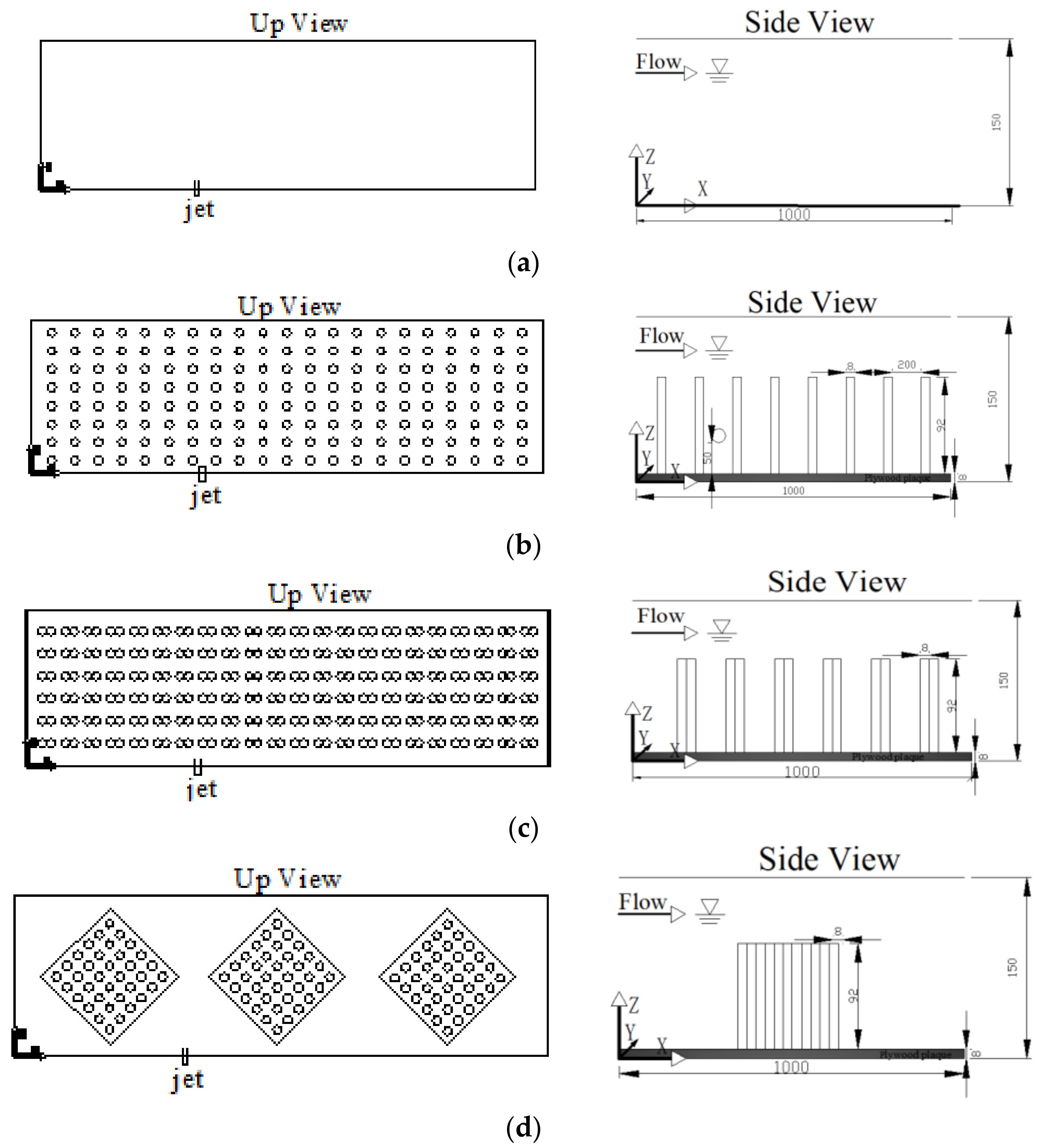
A transparent plexiglass rod was used to simulate rigid vegetation. The rod diameter was 0.8 cm and the rod height was 10 cm. After inserting the plate, the height was 9.2 cm. The plexiglass rod was fixed on a PVC board that was 100 cm long, 30 cm wide, and 0.05 cm thick. The holes for the plexiglass rods were evenly arranged on the plate, and the hole diameters were 0.8 cm. Figure 3 shows a schematic diagram of the vegetation arrangement. In order to effectively measure the flow field around the vegetation using the PIV system, black PVC matte paint was used to blacken the PVC board in order to minimize the impact of PVC surface reflection on the measurements.
3. Results and Discussion
3.1. Distribution of the Average Flow Field in Transverse Jets under Vegetation
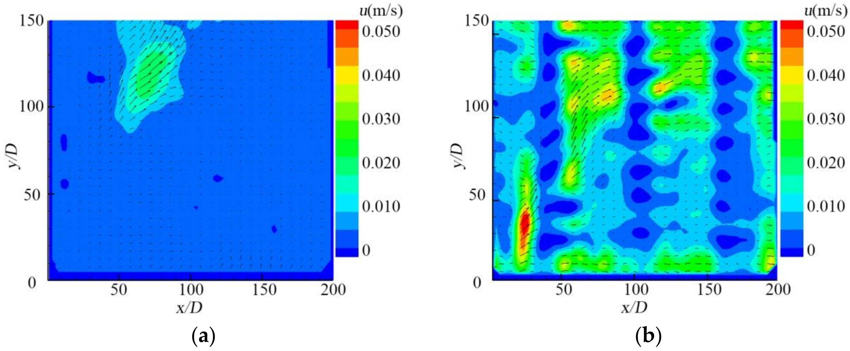
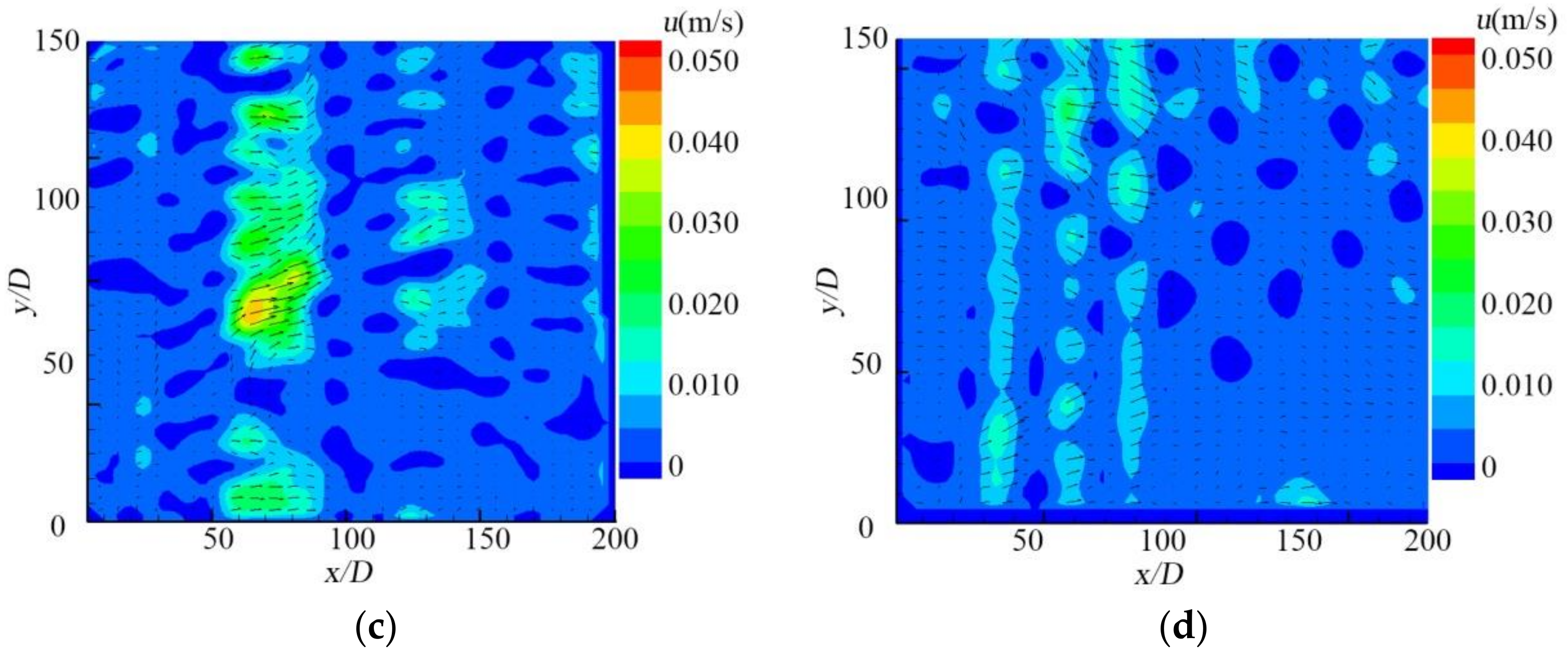
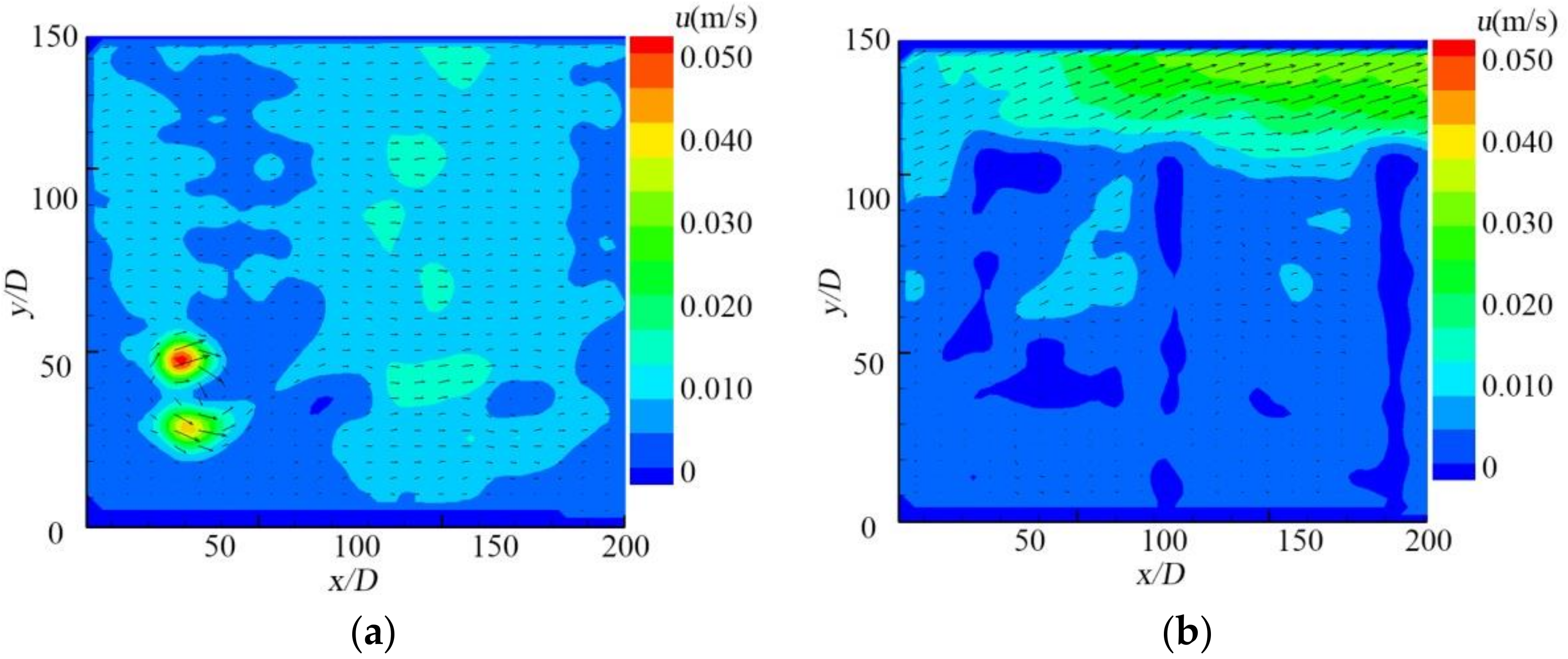
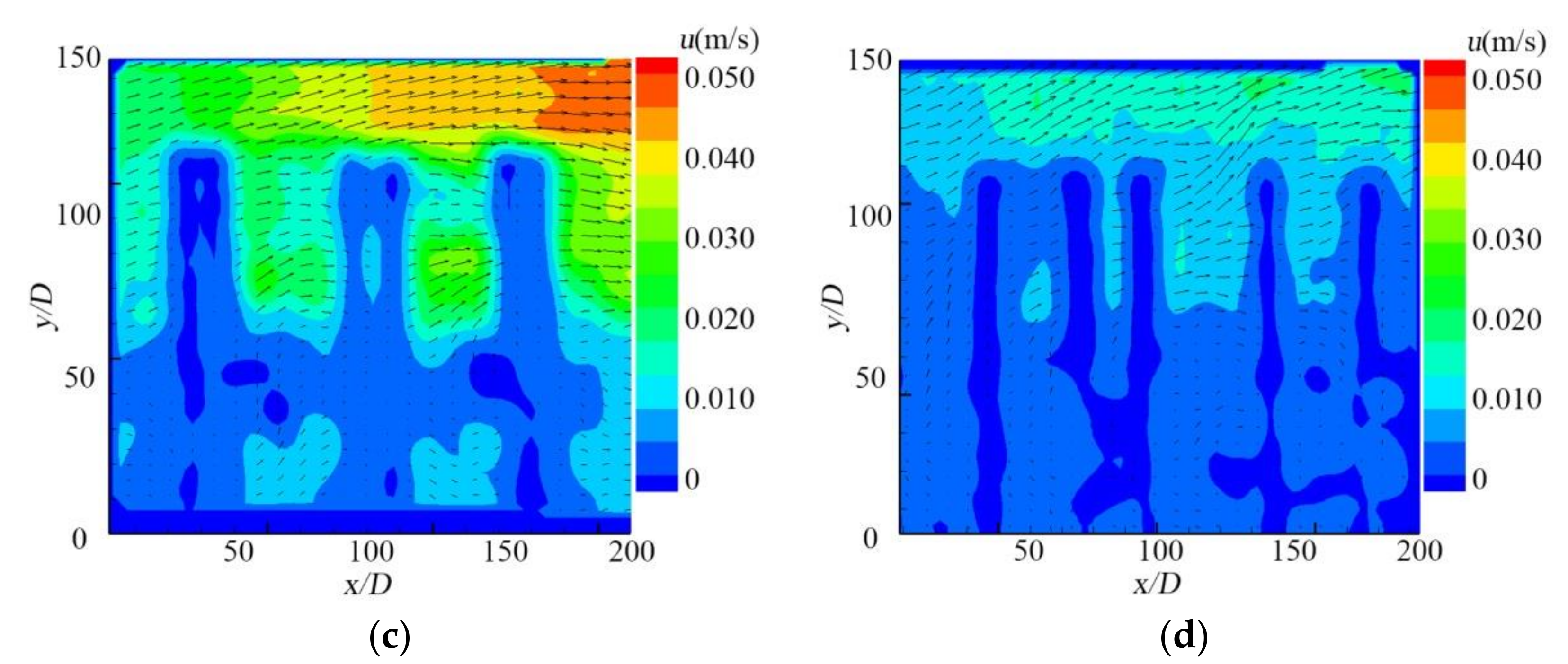
Most research, e.g., Ben Meftah and Mossa [31], Malcangio D [32], White [34], Huai [25], Xiao [35] and Li [36], has focused on the effects of bottom jets, vertical jets, reverse jets, and same-direction jets on non-vegetated environmental bodies of water. These studies found that jets produced obvious structural changes to the water environment. To understand the interaction between jets and vegetation in detail, we first studied the effects of a jet in a waterless environment without vegetation, and then studied the influence of a lateral jet on water with different vegetation arrangements. Figure 4 shows the different flow conditions for the average flow-field distribution of a transverse jet in the horizontal plane z/D = 5, which represents the ratio of water depth to the diameter of the jet hole. Figure 5 shows the average flow-field distribution of a longitudinal section y/D = 10 for the action of vegetation.
Figure 4a shows that for the case in which the vegetation density is zero (V0J1), the water velocity is low at the jet exit, and after the jet leaves the spout at position x/D = 25, y/D = 50, the velocity begins to increase. The jet forms a pair of reverse vortices on the water surface. The velocity changes from a circular shape to a flat pebbly shape and gradually develops into a kidney shape at the jet cross section. As a result of turbulence, the jet velocity is strongly blended with the main velocity. The core velocity gradually increases. When it reaches one half of the river width, u0 begins to bend, a horseshoe vortex appears downstream and a pair of reverse vortices are formed in the wake region of the jet backwater, moving downstream along the flow direction. The jet enters the water body without vegetation, and the speed gradually decreases, which is consistent with the results of Xiao [37] and Ben [33].
Figure 4b shows that with single-row vegetation (V1J1), the maximum jet velocity of umax = 0.065 m/s was reached at the jet nozzle. After the jet passed through the vegetation area, due to the flow around the vegetation, the jet velocity drastically deceased. There was a reverse vortex of varying shapes and sizes, and the velocity approached zero. The velocity gradually increased after the jet passed beyond the vegetation. At position x/D = 100, y/D = 100, large and small horseshoe vortexes appeared.
Figure 4c shows that with double-row vegetation (V2J1), due to the increased vegetation density, the maximum jet velocity of 0.4 m/s appears at position x/D = 60, y/D = 90. The velocity gradually decreased after the jet passed through the vegetation area.
Figure 4d shows that for the V3J1 condition, the vegetation density changed as the vegetation arrangement changed, and the jet had different spot velocities in different places. Through the vegetation area, the velocity was close to zero, and the velocity gradually increased after the jet passed beyond the vegetation. The different vegetation arrangements had a great influence on the jet field. Under the condition of vegetation flow resistance, the velocity changed, and different horseshoe, spot, tail, and reverse vortices appeared at different positions.
To illustrate the variation of the longitudinal velocity of the jet center plane, Figure 5 shows the variation of the dimensionless longitudinal velocity u/ua on the jet center plane for different conditions when the ratio R = 7.57.
Figure 5a shows that, under the conditions of V0J1 without vegetation, a pair of reverse vortices of different sizes appeared near the jet hole along the water depth ratio z/D = 50. Figure 5b shows that the flow velocity was very weak in the vegetation layer, and u/ua in the backflow surface was large, due to the double flow of vegetation around V1J1 and the entrainment of the jet. The dimensionless longitudinal velocity u/ua dropped to zero or was negative. After the jet passed beyond the vegetation layer, the flow entered the free layer and the flow velocity gradually increased near the water surface due to hydrophobic action. Figure 5c shows that with double-row vegetation, the vegetation area and the vegetation arrangement changed. In the vegetation layer, the flow rate changed periodically as the flow velocity changed at a consistent rate as the jet passed through the vegetation. The flow rate dropped sharply. After the jet passed through the vegetation, the decrease in resistance caused the flow rate to increase. In the free layer, the flow rate increased along with the water depth ratio, and the flow velocity was highest at the water surface. Figure 5d shows that for the V3J1 rhombic vegetation, the vegetation arrangement changed from double-row vegetation to diamond-shaped vegetation. Due to the increase in vegetation resistance, the flow velocity of the vegetation layer was almost zero. There was no obstacle in the free layer, so the flow rate increased slowly.
The longitudinal flow velocity with vegetation was similar along the water depth ratio. In the vegetation area, the vegetation arrangement and vegetation resistance were different. In the free area, the flow rate was clearly increased by the absence of vegetation, especially on the water surface. The presence of vegetation increased the surface velocity of the water, and the flow velocity decreased in the interior of the vegetation area and near the bottom of the riverbed. Comparing the time-average flow field diagrams of Figure 4 and Figure 5 under different conditions, it can be seen that rhombic vegetation obstructs the flow velocity most around the lateral jet.
3.2. Vertical Flow Velocity Distribution of a Transverse Jet Along a Vertical Line with Vegetation
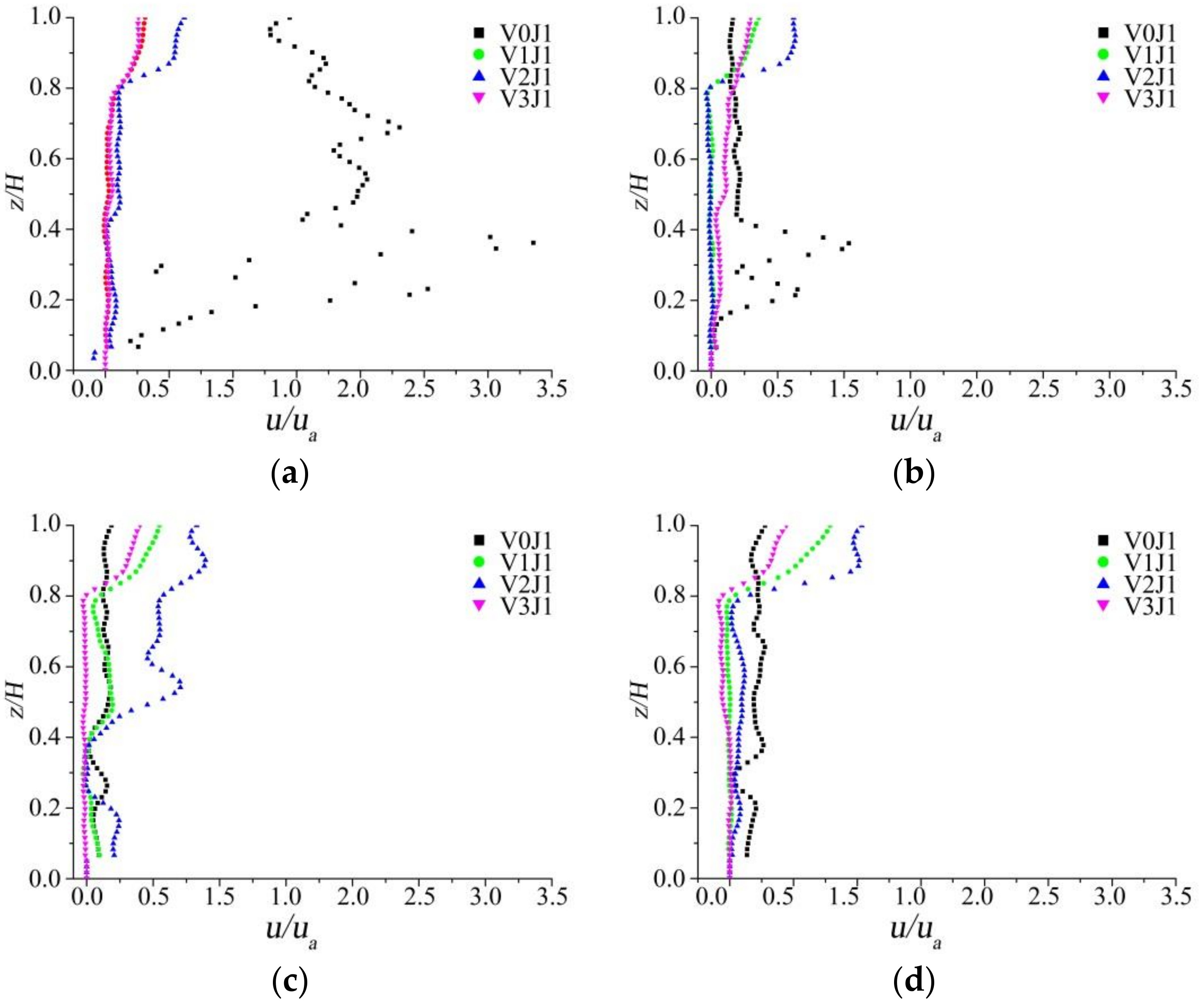
The average flow velocity distribution along the vertical line had obvious regional characteristics. The water flow was greatly affected by the presence of vegetation, and the flow velocity distribution was very complicated. For the study of water flow characteristics in the presence of submerged rigid vegetation, Sanders [3] divided the water flow into a free layer above the vegetation layer and a vegetation layer. The water flow was divided into two layers based on the water depth ratio, with z/H = 0 to z/H = 0.8 being the vegetation layer and z/H = 0.8 to z/H = 1.0 being the free layer. The jet hole position was at z/H = 0.5.
To highlight the significant effects of a cylindrical array of vegetation on the jet flow, we compared some vertical profiles of the dimensionless velocity u/ua between jets discharged into the unobstructed channel (V0J1) and jets discharged into the obstructed and vegetated channels (V1J1 to V3J1) at different downstream positions x/D (see Figure 6).
In Figure 6, u/ua represents the flow ratio and the ordinate z/H represents the water depth ratio. Figure 6a shows a water depth ratio of z/H = 0 to z/H = 0.5 for the V0J1 condition without vegetation. The longitudinal velocity changed drastically in the vertical direction and the velocity distribution showed obvious “S” and anti-“S” types. The velocity distribution results were consistent with the experimental results of the lateral jets obtained by Rajaratnam [14] in a non-vegetated open channel. The flow rate changes significantly around the water depth ratio z/H = 0.5. With vegetation, along the water depth ratio z/H = 0 to z/H = 0.8, for the single-row vegetation and the rhombic vegetation under the V1J1 and V3J1 conditions, the velocities were approximately linear, when the water depth ratio was z/H = 0.8. For double-row vegetation, the velocity had an inflection point. After the inflection point, the velocity increased continuously along the water depth.
Figure 6b shows that the velocity for the V0J1 condition without vegetation was similar to the velocity at the jet hole position x/D = 20, that is, the water depth ratio was from z/H = 0 to z/H = 0.5 when there was no vegetation. The longitudinal velocity changed drastically in the vertical direction, and the velocity distributions were S type and anti-S type. With vegetation, along the water depth ratio z/H = 0 to z/H = 0.8, the vertical velocity along the vertical line for the V3J1 condition was more obvious than for the V1J1 and V2J1 conditions. With the water depth ratio z/H = 0.8, for the V1J1 and V2J1 conditions, the flow exhibited an inflection point, where the free layer was the z/H = 0.8 to z/H = 1.0 interval and the velocity was similar. They followed a logarithmic distribution.
Figure 6c shows that for the V0J1, V1J1 and V3J1 conditions, for water depth ratios of z/H = 0 to z/H = 0.8, the longitudinal flow velocity had S type and anti-S type distributions. Along the water depth ratio z/H = 0.8 to z/H = 1.0, the longitudinal flow velocity was approximately exponential. For the V2J1 condition, which had double-row vegetation, the longitudinal flow velocity showed a significant inflection point at z/H = 0.5.
Figure 6d shows small-amplitude S type and anti-S type distributions for the entire interval without vegetation (V0J1) condition. In the vegetation layer (z/H = 0 to z/H = 0.8) the velocity distribution of the single-row vegetation for the V1J1 condition was approximately linear. For the V2J1 and V3J1 conditions, the flow rate had approximately small-amplitude S type and anti-S type distributions. In the free layer (z/H = 0.8 to z/H = 1.0) for V1J1, V2J1 and V3J1 conditions, the flow rate was logarithmic.
Figure 6a,b show that for no vegetation, the upstream and middle reaches of the jet field exhibited obvious inflection points at z/H = 0.5. The overall trend was S and anti-S distributions. With vegetation, the longitudinal velocity appeared at the vegetation canopy, which is the inflection point at z/H = 0.8. After the flow entered the free layer, the velocity was distributed diagonally to the direction of the water depth. Figure 6c shows that downstream of the jet field for double-row vegetation the velocity changed sharply below the jet orifice (z/H = 0.5), exhibiting a significant trend toward S and anti-S distributions. Figure 6d shows that downstream of the jet field, due to the distance from the jet hole, the velocity varies little with water depth in the vegetation layer, exhibiting small-amplitude S and anti-S distributions. In the free layer, the flow rate followed a logarithmic distribution with respect to the water depth ratio. The above analysis is consistent with the results of Sherif [38] on transverse circular orifice jets. In summary, there are many factors affecting the velocity distribution, such as roughness, jet resistance coefficient, drag coefficient Cd and infiltration height.
3.3. Transverse Jet Motion Trajectory with Vegetation
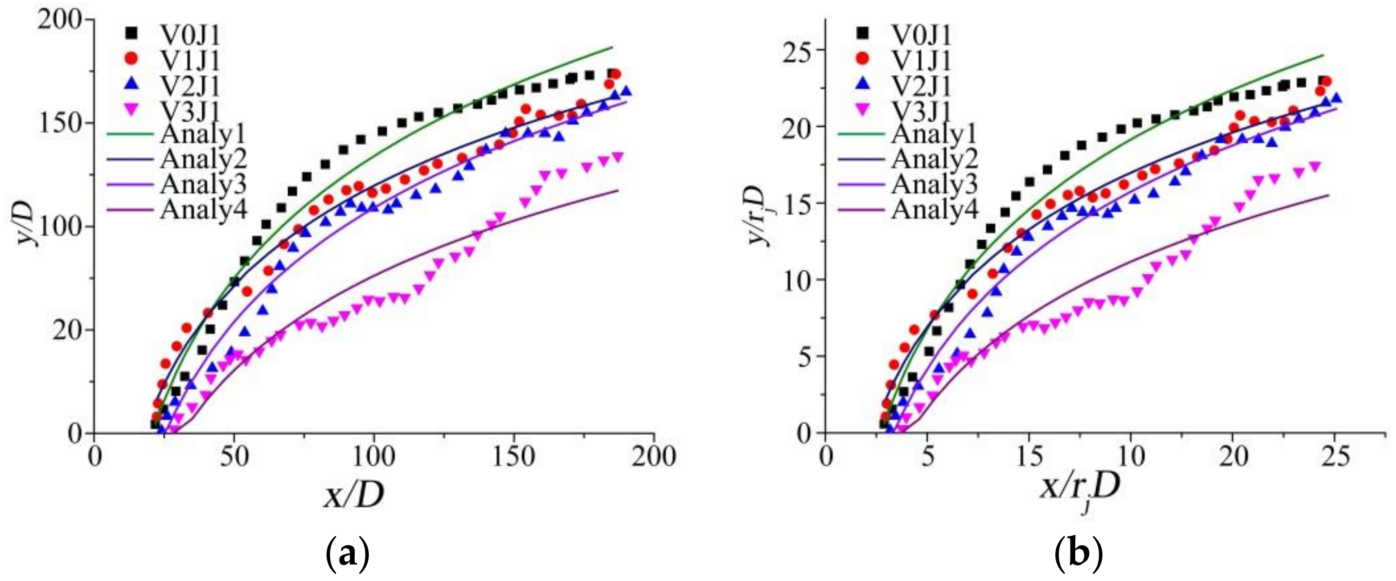
The jet trajectory as the jet enters the cross flow is an important parameter. Numerous experimental and numerical studies have focused on the scale of lateral jet trajectories in open channels without vegetation, but no uniform relationship has been determined for the change with respect to jet trajectory scaling [39]. Using experimental data for the velocity ratio R and the jet incidence angle θ, Lee [15] calculated and analyzed the vertical jet flow field and concentration field in the cross flow. Based on the blend length scale theory of Wright [40] and Kundsen [41], Gao [19] analyzed the mixing lengths of different flow regions in the countercurrent. To account for the bending variation of the jet trajectory being related to the flow velocity ratio, Ben [32] used the dimensionless D and the dimensionless rjD to analyze jet trajectory changes. The study investigated vegetation and no vegetation scenarios, and was conducted to analyze the changes in the transverse jet trajectory. To further analyze the jet trajectory, Kamotani [11] proposed an alternative scaling, normalizing the coordinates with D, that is, x/D and y/D, and went on to obtain a power law of the jet trajectories in the form of:
where A and B are experimental coefficients. Margason [42] reviewed several correlations and concluded that much of the data could be collapsed by normalizing coordinates with the product rjD, leading to a simple power law trajectory in the form of:
A power law similar to Equation (2) was also proposed by Pratte, B. [43], based on their dimensional analysis for a jet with rjD ranging from 5 to 35. New et al. [39] indicated that some researchers affirmed that jet trajectories are best scaled with rjD instead of D or rj2D.The formula was as follows [42]:
In Equation (3), the value a ranged from 65.84 to 85.2, and b ranged from 198.43 to 258.89.
Figure 7 shows the jet motion trajectory for different working conditions. In Figure 7a, x/D represents the water flow ratio, and y/D represents the river width ratio. In Figure 7b, x/rjD represents the water flow ratio, y/rjD represents the river width ratio and rj represents the ratio of the ambient flow rate to the jet flow rate. V0J1 represents the transverse jet trajectory without vegetation, and V1J1 to V3J1 represent the transverse jet trajectories with vegetation.
With vegetation, the results from the theoretical analysis of the jet trajectory are in agreement with the experimental results. There are some differences in the lateral jet trajectory for vegetated conditions. Because of the resistance of the vegetation and the pressure difference of the jet, for the vegetated conditions, the transverse jet trajectory is more likely to bend than in the case with no vegetation. The results demonstrate that under the same hydraulic conditions, the lateral jet in the open channel has a higher penetration ability than it does with no vegetation.
3.4. Turbulence Intensity
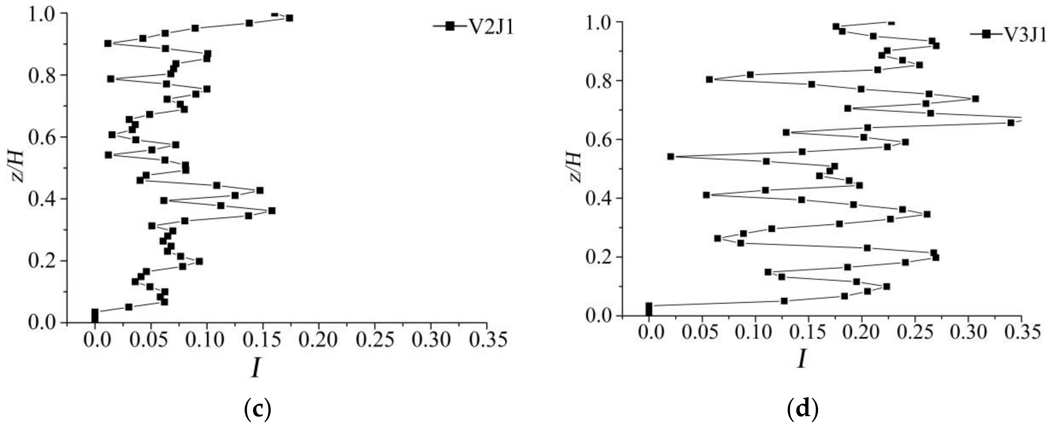
To understand the influence of the lateral jet in an open channel on a surrounding flow field, it is necessary to study turbulence, which affects the intensity of the flow velocity fluctuation. In the statistical theory of turbulence, the second-order central moment of any one of the pulsating velocity components is used to express the degree of dispersion of the instantaneous velocity around the time-average velocity, and its physical meaning is twice the mean value of the pulsating kinetic energy per unit mass of water. The turbulence intensity is divided by the characteristic flow rate to obtain the relative turbulence intensity to synthesize the turbulence intensity:
The turbulence intensity is calculated using the combined flow rates in both the x and z directions.
where U is the average vertical velocity of the transverse jet in the open channel without vegetation.
Figure 8 shows the relative turbulence intensity along the vertical line for four different conditions. The abscissa represents the relative turbulence intensity, and the ordinate represents the water depth ratio. For the V0J1 condition, due to the jet pressure difference, the turbulent intensity of the jet near z/H = 0.5 is weaker than the turbulent flow above the bottom of the tank and above the jet orifice. For the V3J1 condition, which is affected by the rhombic vegetation, the distribution of turbulence intensity along the water depth ratio z/H = 0.7 is 0.5 above the turbulence intensity at the water depth ratio of z/H = 0.8. This is a much greater difference than for V1J1, V2J1 and V3J1. In conclusion, for vegetated conditions, the transverse jet has obvious anisotropic turbulence characteristics in open channel flow.
3.5. Reynolds Stress
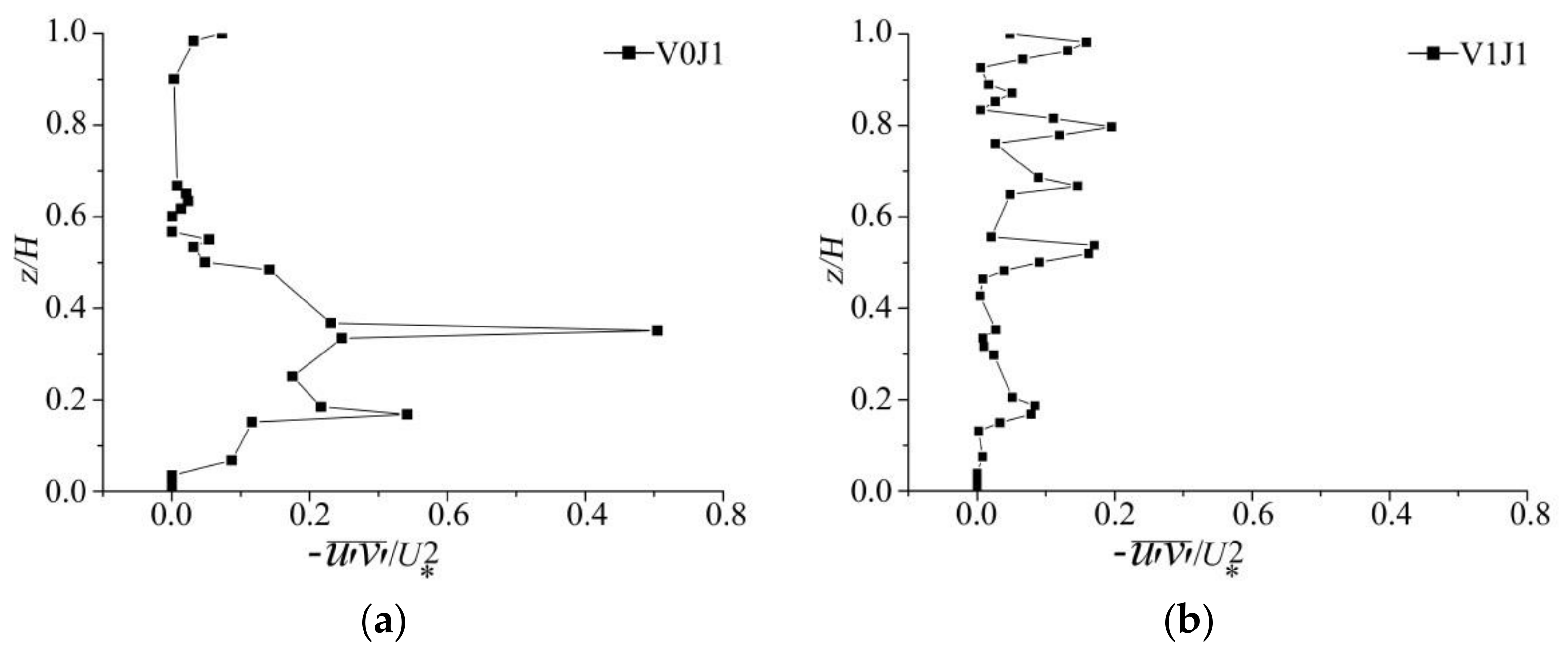
The Reynolds stress is generated due to the uneven distribution of the flow velocity in the flow field. The greater the Reynolds stress is, the more uneven the flow velocity distribution at that point, indicating that the turbulence is more severe. The Reynolds stress τ of a two-dimensional open channel can be expressed as:
where u′ and v′ represent the longitudinal and vertical pulsation velocities, respectively.
Figure 9 shows the Reynolds stress along the vertical line. The abscissa represents the Reynolds stress after nondimensionalization, and the ordinate z/H represents the water depth ratio. For the V0J1 condition without vegetation, due to the existence of jet flow resistance the turbulent exchange is strong in the jet hole (z/H = 0.3 to z/H = 0.5) and the Reynolds stress peak reaches 0.7. For the V1J1 condition with single-row vegetation, the Reynolds stress peaked in the top area of the vegetation (near z/H = 0.8). With the double-row vegetation of V2J1, the Reynolds stress is the largest near the water surface. For the V3J1 condition with its rhombic vegetation, the peak of the Reynolds stress appeared in the top area of vegetation (near z/H = 0.8). Comparing the four working conditions, it can be seen that when the water depth ratio is z/H = 0 to z/H = 0.1, due to the influence of vegetation resistance and groove bottom roughness the Reynolds stress is almost zero. Comparing V1J1, V2J1 and V3J1, it can be seen that the distribution trend of the Reynolds stress in single-row vegetation and rhombic vegetation above the vegetation layer is the same, while the double-row vegetation has the largest Reynolds stress near the water surface, which is the result of the large flow gradient.
4. Conclusions
Many researchers have studied the flow characteristics of bottom jets, coflow jets or reverse jets in open channels, and others have used bottom jets to study the flow characteristics of open channel under the action of a single vegetation. However, the published data on the flow characteristics in open channels produced by lateral jets are very limited. Based on a round, lateral jet flow, the present work focuses on the characteristics of open channel flow under three vegetations and a comparison is made with the flow field without vegetation. High-frequency PIV was used to measure flow fields with a lateral jet in three different arrangements with vegetation, and a comparison was made to a flow field without vegetation. The time-averaged flow velocity, turbulence intensity and Reynolds stress were analyzed. The main conclusions are as follows:
- The study of the time-average flow rates shows that vegetation significantly disturbs the flow field around a lateral jet. Without vegetation, due to turbulent entrainment, the jet flow rate was strongly blended with the main flow rate and the flow velocity in the core region was increased. The flow rate decreased in the downstream direction. Due to the flow around the vegetation, the flow velocity distribution changed significantly, exhibiting horseshoe, spotted, wake and reverse vortices of different sizes in different locations. A comparison of four different vegetation arrangements showed that the vegetation arrangement influences the jet flow field, most obviously for the rhombic arrangement.
- According to the analysis of the vertical flow velocity, the flow velocity in the inner region of the vegetation and near the bottom of the trough was reduced. The flow velocity along the water depth was of S and anti-S types, and the flow velocity of the free layer was approximately logarithmic.
- By comparing the jet trajectories under different conditions, it was found that jet penetration was significantly greater in the cases with vegetation than for the case without vegetation, and the jet trajectory was more curved for the diamond vegetation arrangement.
- The analysis of turbulence intensity and Reynolds stress showed that the flow gradient was very large due to the strong water flow turbulence, and the Reynolds stress peaks at the top of the vegetation (z/H = 0.8) and near the water surface. We found that the relative turbulence intensity varies most along the water depth ratio for the rhombic arrangement of vegetation.
Author Contributions
Conceptualization, S.T.; Methodology, S.T.; Software, S.T. and K.C.; Validation, S.T., M.F. and B.Z.; Formal Analysis, W.W.; Investigation, S.T.; Resources, S.T.; Data Curation, S.T.; Writing—Original Draft Preparation, S.T.; Writing—Review & Editing, S.T.; Visualization, S.T. and K.C.; Supervision, M.F. and B.Z.; Project Administration, S.T. and M.F.; Funding Acquisition, S.T. and M.F.
Funding
This research was financially supported by the Natural Science Foundation of China (Fund No. 51679191). In particular, it was funded by the Xi’an University of Technology Doctoral Innovation Fund (Fund No.310-252071507.
Acknowledgments
Additionally, good suggestions and comments from Hansong Tang (The City University of New York), Zhichang Zhang and Guodong Li (School of Water Resources and Hydroelectric Engineering, Xi’an University of Technology) are greatly appreciated.
Conflicts of Interest
The authors declare no conflict of interest.
References
- Hussein, J.; Capp, S.P.; George, W.K. Velocity measurements in a high-Reynolds-number, momentum-conserving, axisymmetric, turbulent jet. J. Fluid Mech. 1994, 258, 31–75. [Google Scholar] [CrossRef]
- Fischer, B.H.; List, E.J.; Koh, R.C.Y.; Imberger, J.; Brooks, N.H. Chapter 6—Mixing in reservoirs. In Mixing Inland Coastal Waters; Elsevier: Amsterdam, The Netherlands, 1979. [Google Scholar]
- Sanders, H.J.P.; Sarh, B.; Gökalp, I. Variable density effects in axisymmetric isothermal turbulent jets: A comparison between a first- and a second-order turbulence model. Int. J. Heat Mass Transf. 1997, 40, 823–842. [Google Scholar] [CrossRef]
- Cha, J.; Lim, S.; Kim, T.; Shin, W.G. The effect of the Reynolds number on the velocity and temperature distributions of a turbulent condensing jet. Int. J. Heat Fluid Flow 2017, 67, 125–132. [Google Scholar] [CrossRef]
- Coletti, F.; Benson, M.J.; Ling, J.; Elkins, C.J.; Eaton, J.K. Turbulent transport in an inclined jet in crossflow. Int. J. Heat Fluid Flow 2013, 43, 149–160. [Google Scholar] [CrossRef]
- Fox, J.F.; Smith, M.M.; Nuttall, G.A. Kaplans Essentials of Cardiac Anesthesia; Elsevier: Amsterdam, The Netherlands, 2018; pp. 426–472. [Google Scholar]
- Jirka, H.G.; Bleninger, T.; Burrows, R.; Larsen, T. Environmental Quality Standards in the EC-Water Framework Directive: Consequences for Water Pollution Control for Point Sources; KIT: Karlsruhe, Germany, 2004. [Google Scholar]
- Yang, W.; Choi, S.U. Impact of stem flexibility on mean flow and turbulence structure in depth-limited open channel flows with submerged vegetation. J. Hydraul. Res. 2009, 47, 445–454. [Google Scholar] [CrossRef]
- Freund, J.B. Noise sources in a low-Reynolds-number turbulent jet at Mach 0.9. J. Fluid Mech. 2001, 438, 277–305. [Google Scholar] [CrossRef]
- Yu, C. Introduction to Environmental Fluid Mechanics; Tsinghua University Press: Beijing, China, 1992. [Google Scholar]
- Kamotani, Y.; Greber, I. Experiments on a turbulent jet in a crossflow. AIAA J. 1972, 30, 1425–1429. [Google Scholar] [CrossRef]
- Fischer, H.B.; List, J.E.; Koh, C.R.; Imberger, J.; Brooks, N.H. Chapter 9—Turbulent Jets and Plumes. In Mixing in Inland and Coastal Waters; Elsevier Inc.: New York, NY, USA, 1979; pp. 315–389. [Google Scholar]
- Smith, S.H.; Mungal, M.G. Mixing, structure and scaling of the jet in cross-flow. J. Fluid Mech. 1998, 357, 83–122. [Google Scholar] [CrossRef]
- Rajaratnam, N. Erosion by turbulent jets. J. Hydraul. Res. 1981, 19, 339–358. [Google Scholar] [CrossRef]
- Lee, J.; Kuang, C.; Chen, G. The structure of a turbulent jet in crossflow—Effect of jet-to-crossflow velocity. China Ocean Eng. 2002, 16, 1–20. [Google Scholar]
- Zeng, Y.; Yan, W. Experimental study of three-dimensional circular vertical buoyant jet characteristics in a flowing environment. Exp. Fluid Mech. 2005, 19, 39–46. [Google Scholar]
- Zhang, C.; Jian, M.; Qin, C.; Yang, D. Numerical simulation of vertical circular pure jet in shallow water environment. J. Zhejiang Univ. 2006, 12, 2163–2167. [Google Scholar]
- Li, W.; Gu, J.; Yan, C.; Wang, Y. Experimental study on jet trajectory and diffusion characteristics in crossflow based on PIV. Hydrodyn. Res. Prog. 2018, 33, 207–215. [Google Scholar]
- Gao, M.; Huai, W.; Xiao, Y.; Yang, Z.; Ji, B. Large eddy simulation of a vertical buoyant jet in a vegetated channel. Int. J. Heat Fluid Flow 2018, 70, 114–124. [Google Scholar] [CrossRef]
- Meftah, B.M.; de Serio, F.; Mossa, M. Hydrodynamic behavior in the outer shear layer of partly obstructed open channels. Phys. Fluids 2014, 26, 1624–1635. [Google Scholar] [CrossRef]
- Yang, K.; Liu, X.; Cao, S.; Zhang, Z. The turbulent characteristics of floodplain flow in a complex river channel under the action of vegetation. J. Hydraul. Eng. 2005, 36, 1263–1268. [Google Scholar]
- Nepf, H.M.; Vivoni, E.R. Flow structure in depth-limited, vegetated flow. J. Geophys. Res. Oceans 2000, 105, 28547–28557. [Google Scholar] [CrossRef] [Green Version]
- Zhang, M.; Chen, G.; Xu, L.; Li, Z. Application of PIV technology in submerged jet of experimental model of plunge pool. In Proceedings of the National Conference on Experimental Fluid Mechanics, Sydney, Australia, 13–17 December 2004. [Google Scholar]
- Li, C.; Yan, W.; Yang, H. Study on the characteristics of non-submerged rigid vegetation flow in curved corners. J. Huazhong Univ. Sci. Technol. 2012, 40, 49–53. [Google Scholar]
- Wen, H.; Yu, N.A.; Han, T.; Ai, L.I. Experimental study on vertical turbulent jet discharged from the bottom of shallow water. J. Hydraul. Eng. 2002, 13, 26–30. [Google Scholar]
- Li, R. Effect of tall vegetations on flow and sediment. J. Hydraulic Div. ASCE 1973, 99, 793–814. [Google Scholar]
- Lindner, K.; Saenger, W. Crystal and molecular structure of cyclohepta-amylose dodecahydrate. Carbohydr. Res. 1982, 99, 103–115. [Google Scholar] [CrossRef]
- Murphy, E.; Ghisalberti, M.; Nepf, H. Model and laboratory study of dispersion in flows with submerged vegetation. Water Resour. Res. 2007, 43, 687–696. [Google Scholar] [CrossRef]
- De Serio, F.; Meftah, M.B.; Mossa, M.; Termini, D. Experimental investigation on dispersion mechanisms in rigid and flexible vegetated beds. Adv. Water Resour. 2017. [Google Scholar] [CrossRef]
- Meftah, M.B.; Mossa, M. Prediction of channel flow characteristics through square arrays of emergent cylinders. Phys. Fluids 2013, 25, 13–25. [Google Scholar] [CrossRef]
- Meftah, M.B.; De Serio, F.; Malcangio, D.; Mossa, M.; Petrillo, A.F. Experimental study of a vertical jet in a vegetated crossflow. J. Environ. Manag. 2015, 164, 19–31. [Google Scholar] [CrossRef] [PubMed]
- Malcangio, D.; Meftah, M.B.; Chiaia, G.; De Serio, F.; Mossa, M.; Petrillo, A. Experimental Studies on Vertical Dense Jets in a Crossflow; Taylor & Francis Group: Oxford, UK, 2016. [Google Scholar]
- Meftah, M.B.; Mossa, M. Turbulence measurement of vertical dense jets in crossflow. Water 2018, 10, 286. [Google Scholar] [CrossRef]
- White, B.L.; Nepf, H.M. Shear instability and coherent structures in shallow flow adjacent to a porous layer. J. Fluid Mech. 2007, 593, 1–32. [Google Scholar] [CrossRef]
- Xiao, Y.; Tang, H.; Hua, M.; Wang, Z. Experimental study on the mixing characteristics of co-directional jets. Adv. Water Sci. 2006, 17, 512–517. [Google Scholar]
- Li, Z.; Yan, W.; Qian, Z. Numerical simulation of radial turbulent jet in still water environment. J. Hydraul. Eng. 2009, 40, 1320–1325. [Google Scholar]
- Xiao, Y.; Lei, M.; Li, K.; Liu, G.; Yan, J. Experimental study on flow characteristics of porous jets in cross-flows. Adv. Water Sci. 2012, 23, 390–395. [Google Scholar]
- Sherif, S.A.; Pletcher, R.H. Measurements of the flow and turbulence characteristics of round jets in crossflow. J. Fluids Eng. 1989, 111, 165–171. [Google Scholar] [CrossRef]
- New, T.H.; Lim, T.T.; Luo, S.C. Effects of jet velocity profiles on a round jet in cross-flow. Exp. Fluids 2006, 40, 859–875. [Google Scholar] [CrossRef]
- Wright, S.J. Effects of Ambient Crossflows and Density Stratification on the Characteristic Behavior of Round, Turbulent Bouyant Jets; California Institute of Technology: Pasadena, CA, USA, 1977. [Google Scholar]
- Knudsen, M. Buoyant Horizontal Jets in an Ambient Flow. Ph.D. Thesis, University of Canterbury, Canterbury, UK, 1988. [Google Scholar]
- Margason, R.J. The Path of a Jet Directed at Large Angles to a Subsonic Stream; Langley Research Center: Hampton, VA, USA, 1968. [Google Scholar]
- Pratte, B.D.; Baines, W.D. Profiles of the round turbulent jet in a cross-flow. J. Hydraulic Div. 1967, 92, 53–64. [Google Scholar]
Figure 1.
Sketch of the experimental setup.

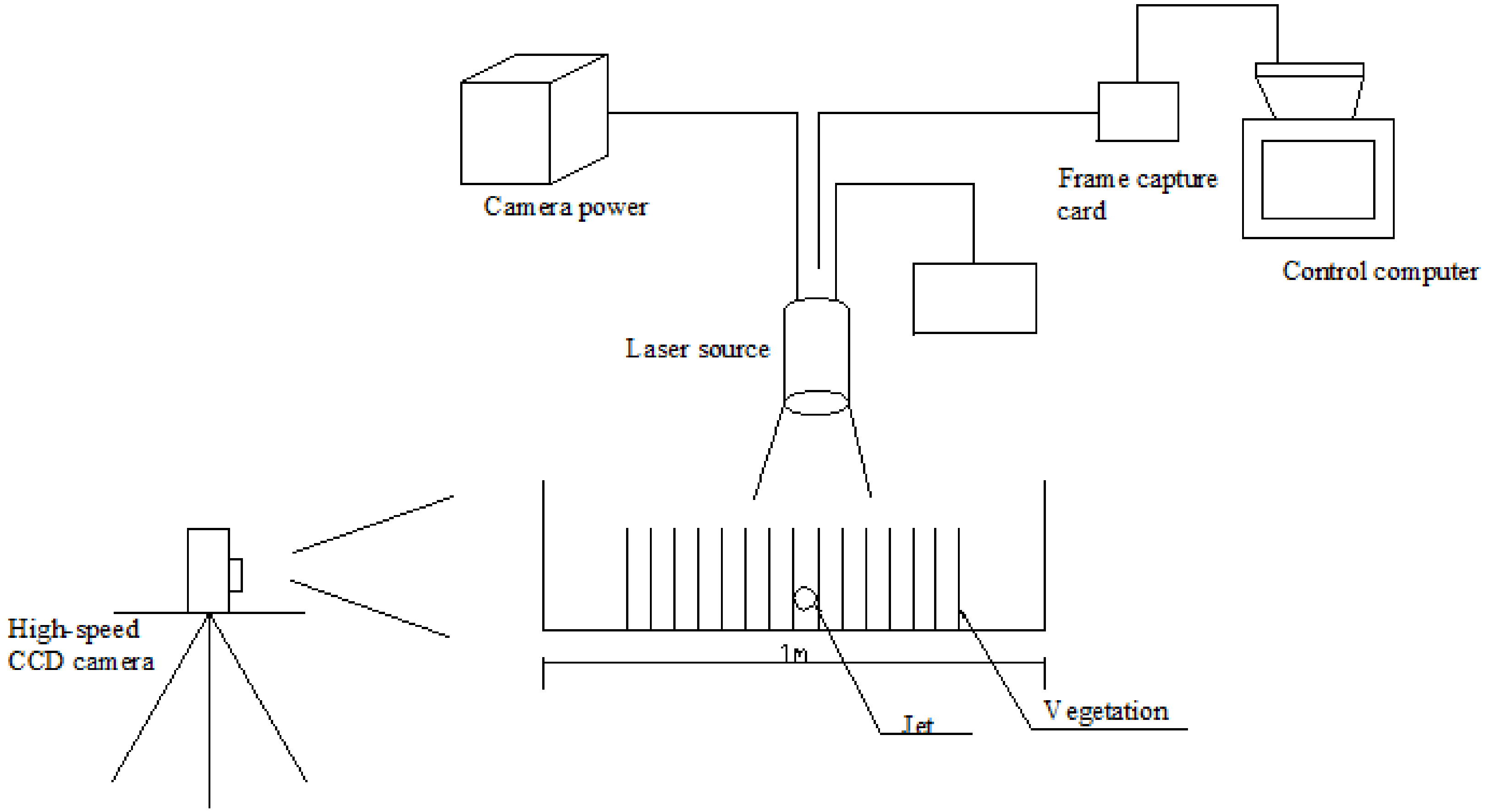
Figure 2.
PIV measurement system and photo area.

Figure 3.
Schematic diagrams of the vegetation arrangement. (a) No vegetation arrangement; (b) Single row vegetation arrangement; (c) Double row vegetation arrangement; (d) Diamond vegetation arrangement.
Figure 3.
Schematic diagrams of the vegetation arrangement. (a) No vegetation arrangement; (b) Single row vegetation arrangement; (c) Double row vegetation arrangement; (d) Diamond vegetation arrangement.

Figure 4.
The different flow conditions for the average flow-field distribution of a transverse jet in the horizontal plane z/D = 5. (a) vector map of Vxy for run V0J1; (b) vector map of Vxy for run V1J1; (c) vector map of Vxy for run V2J1; (d) vector map of Vxy for run V3J1. (Note: Color indicates the speed: blue represents the lowest speed, and red represents the highest speed.)


Figure 5.
The average flow field distribution of a longitudinal section y/D = 10 under the action of vegetation. (a) vector map of Vxz for run V0J1; (b) vector map of Vxz for run V1J1; (c) vector map of Vxz for run V2J1; (d) vector map of Vxz for run V3J1.
Figure 5.
The average flow field distribution of a longitudinal section y/D = 10 under the action of vegetation. (a) vector map of Vxz for run V0J1; (b) vector map of Vxz for run V1J1; (c) vector map of Vxz for run V2J1; (d) vector map of Vxz for run V3J1.


Figure 6.
Vertical flow velocity distribution of transverse jets at the different positions x/D under different conditions. (a)Velocity distribution along the vertical at x/D = 20; (b) Velocity distribution along the vertical at x/D = 25; (c) Velocity distribution along the vertical at x/D = 50; (d) Velocity distribution along the vertical at x/D = 75.

Figure 7.
Jet axis motion trajectory. (a) Coordinates are normalized by D; (b) Coordinates are normalized by rjD.
Figure 7.
Jet axis motion trajectory. (a) Coordinates are normalized by D; (b) Coordinates are normalized by rjD.

Figure 8.
Vertical distribution of relative turbulence intensity. (a) The dimensionless turbulence intensity for run V0J1; (b) The dimensionless turbulence intensity for run V1J1; (c) The dimensionless turbulence intensity for run V2J1; (d) The dimensionless turbulence intensity for run V3J1.
Figure 8.
Vertical distribution of relative turbulence intensity. (a) The dimensionless turbulence intensity for run V0J1; (b) The dimensionless turbulence intensity for run V1J1; (c) The dimensionless turbulence intensity for run V2J1; (d) The dimensionless turbulence intensity for run V3J1.


Figure 9.
Reynolds stress vertical distribution. (a) The dimensionless Reynolds stress for V0J1; (b) The dimensionless Reynolds stress for V1J1; (c) The dimensionless Reynolds stress for V2J1; (d) The dimensionless Reynolds stress for V3J1.
Figure 9.
Reynolds stress vertical distribution. (a) The dimensionless Reynolds stress for V0J1; (b) The dimensionless Reynolds stress for V1J1; (c) The dimensionless Reynolds stress for V2J1; (d) The dimensionless Reynolds stress for V3J1.


Table 1.
Parameters of the experiments.
| Run | Condition | Q (m3/h) | H (m) | ua (m/s) | u0 (m/s) | R | Re | X (m) | Y (m) |
|---|---|---|---|---|---|---|---|---|---|
| V0J1 | No | 6 | 0.15 | 0.037 | 0.28 | 7.57 | 2791 | ||
| V1J1 | Single row | 6 | 0.15 | 0.037 | 0.28 | 7.57 | 2791 | 0.03 | 0.02 |
| V2J1 | Double row | 6 | 0.15 | 0.037 | 0.28 | 7.57 | 2791 | 0.02 | 0.035 |
| V3J1 | Diamond | 6 | 0.15 | 0.037 | 0.28 | 7.57 | 2791 | 0.02 | 0.02 |
© 2018 by the authors. Licensee MDPI, Basel, Switzerland. This article is an open access article distributed under the terms and conditions of the Creative Commons Attribution (CC BY) license (http://creativecommons.org/licenses/by/4.0/).
Share and Cite
MDPI and ACS Style
Teng, S.; Feng, M.; Chen, K.; Wang, W.; Zheng, B. Effect of a Lateral Jet on the Turbulent Flow Characteristics of an Open Channel Flow with Rigid Vegetation. Water 2018, 10, 1204. https://doi.org/10.3390/w10091204
AMA Style
Teng S, Feng M, Chen K, Wang W, Zheng B. Effect of a Lateral Jet on the Turbulent Flow Characteristics of an Open Channel Flow with Rigid Vegetation. Water. 2018; 10(9):1204. https://doi.org/10.3390/w10091204
Chicago/Turabian StyleTeng, Sufen, Minquan Feng, Kailin Chen, Weijie Wang, and Bangmin Zheng. 2018. "Effect of a Lateral Jet on the Turbulent Flow Characteristics of an Open Channel Flow with Rigid Vegetation" Water 10, no. 9: 1204. https://doi.org/10.3390/w10091204
Note that from the first issue of 2016, this journal uses article numbers instead of page numbers. See further details here.