An Integrated Hydrological-Hydraulic Model for Simulating Surface Water Flows of a Shallow Lake Surrounded by Large Floodplains

 , , and
Abstract
:1. Introduction
2. Hydrological-Hydraulic Integrated Model
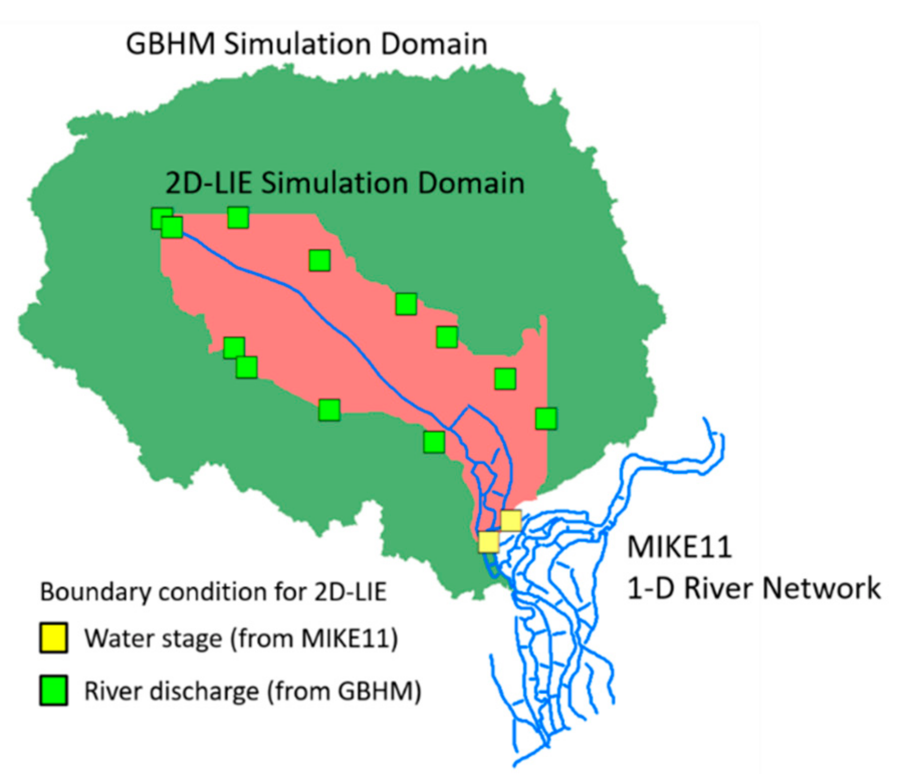
2.1. Model Structure
2.2. GBHM
2.3. MIKE11
2.4. Local Inertial Model
3. Numerical Scheme for the 2-D LIE
3.1. Discretization
3.2. Stability Analysis Results
4. Application
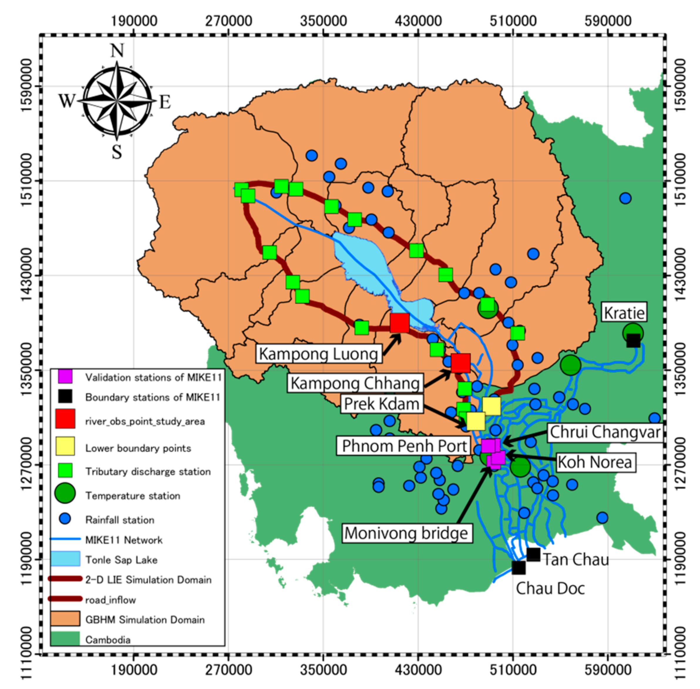
4.1. Study Site
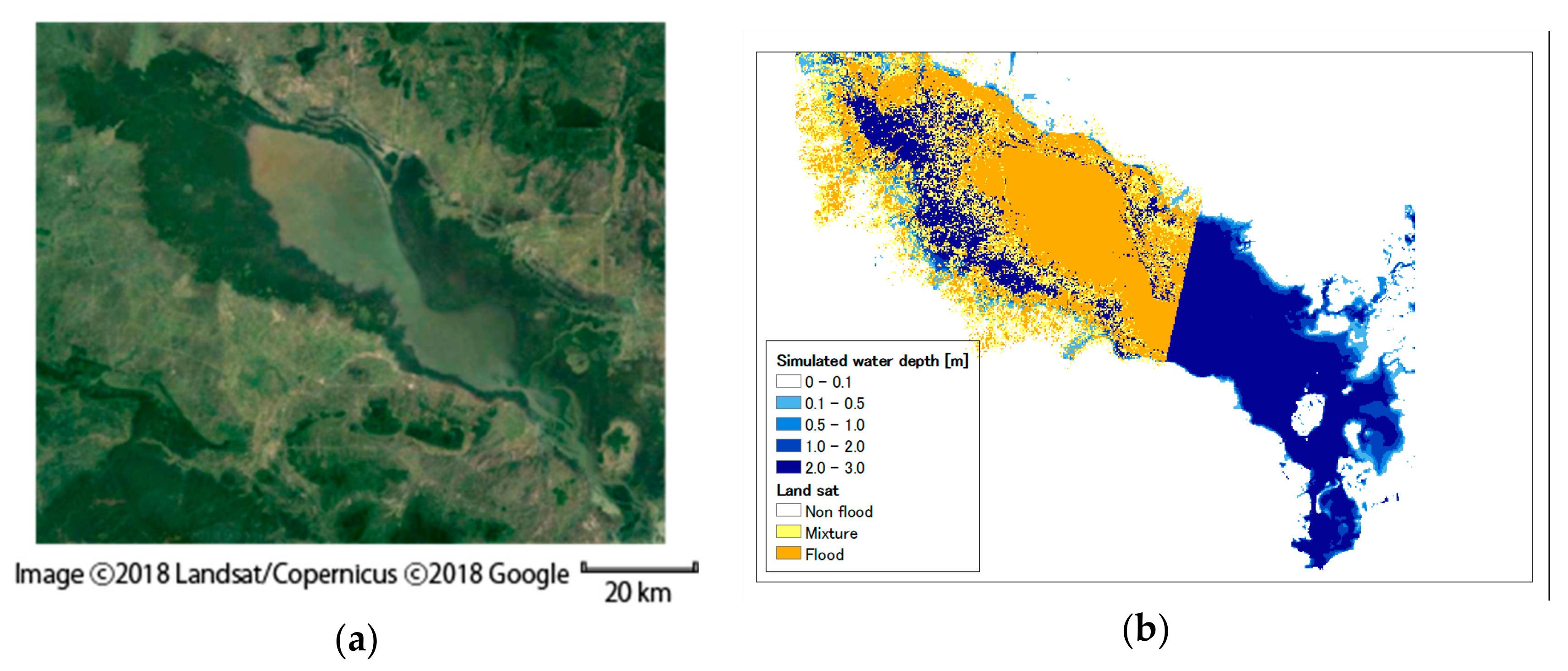
4.2. Remote Sensing
4.3. Model Setup in the Tonle Sap Lake
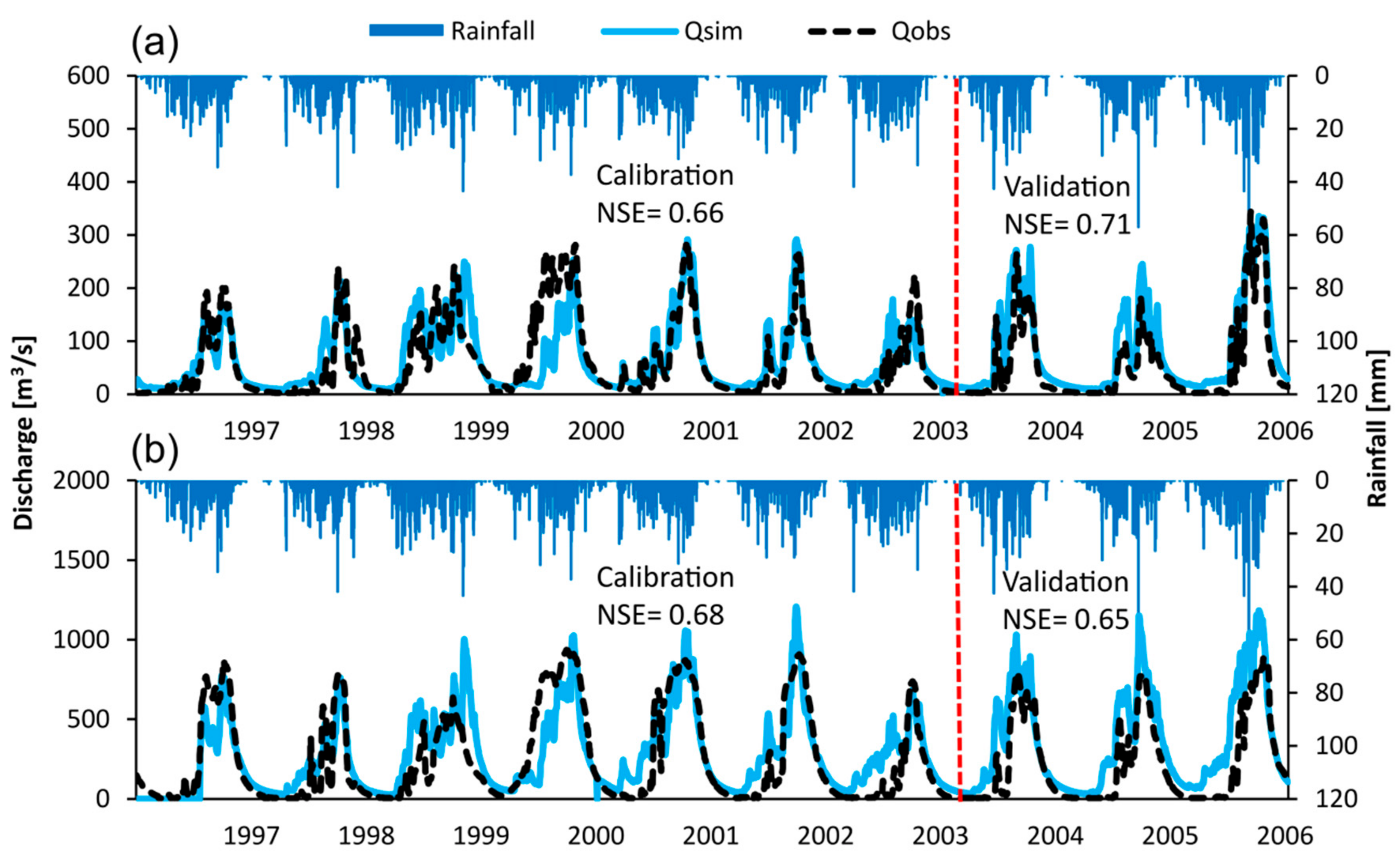
4.3.1. Hydrological Model GBHM
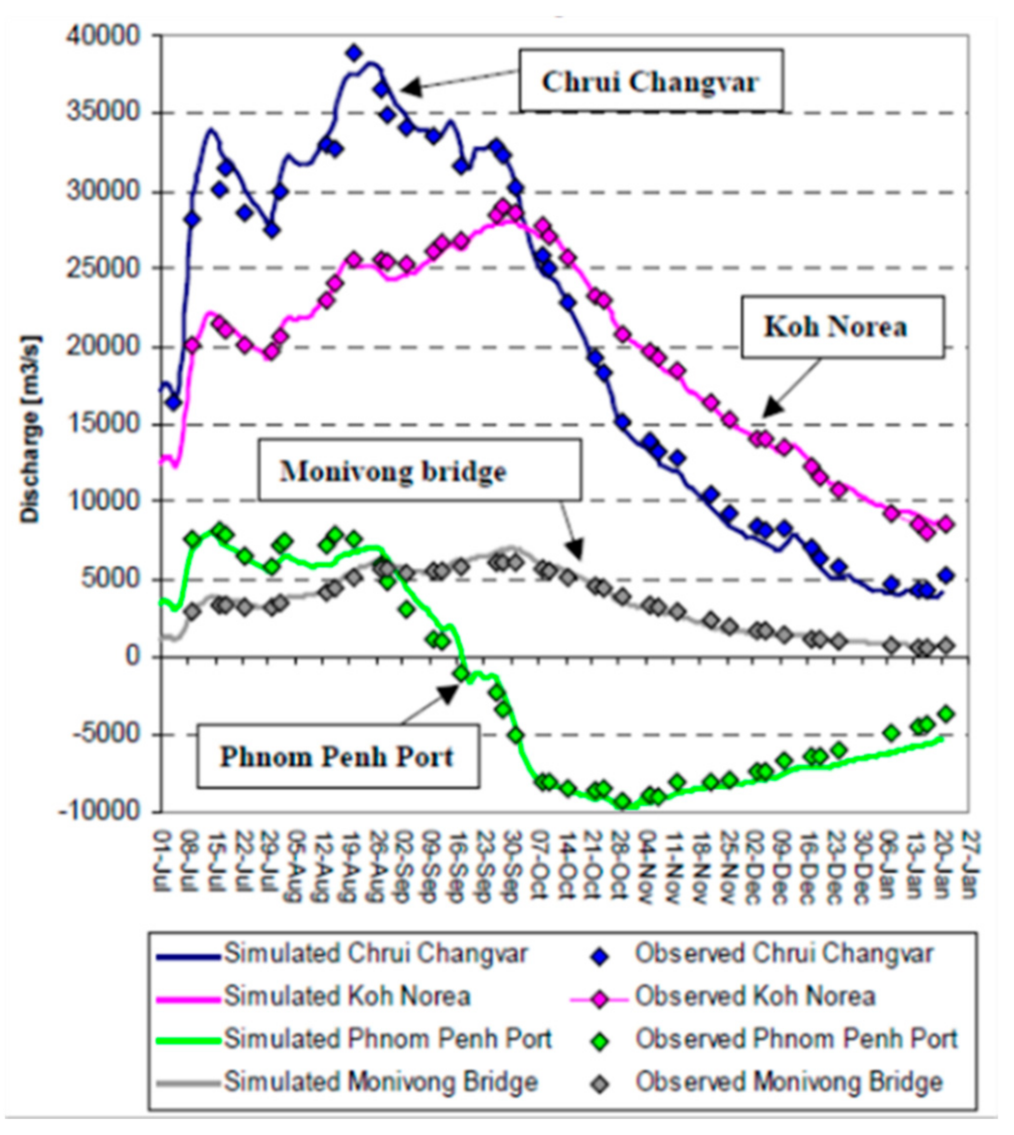
4.3.2. 1-D River and Lake Routing Model MIK11
4.3.3. 2-D Local Inertial Equation
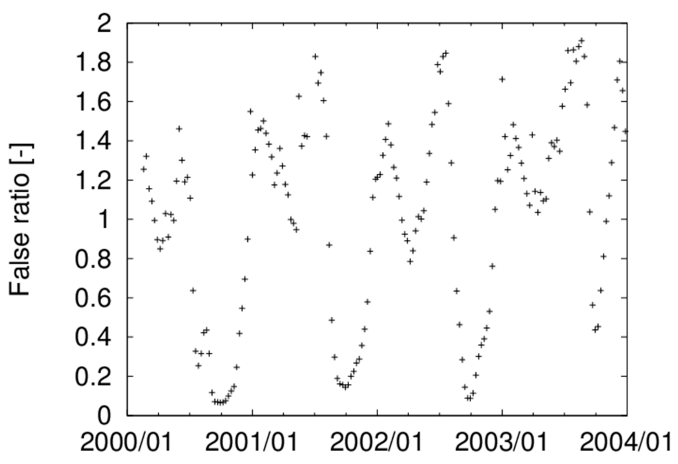
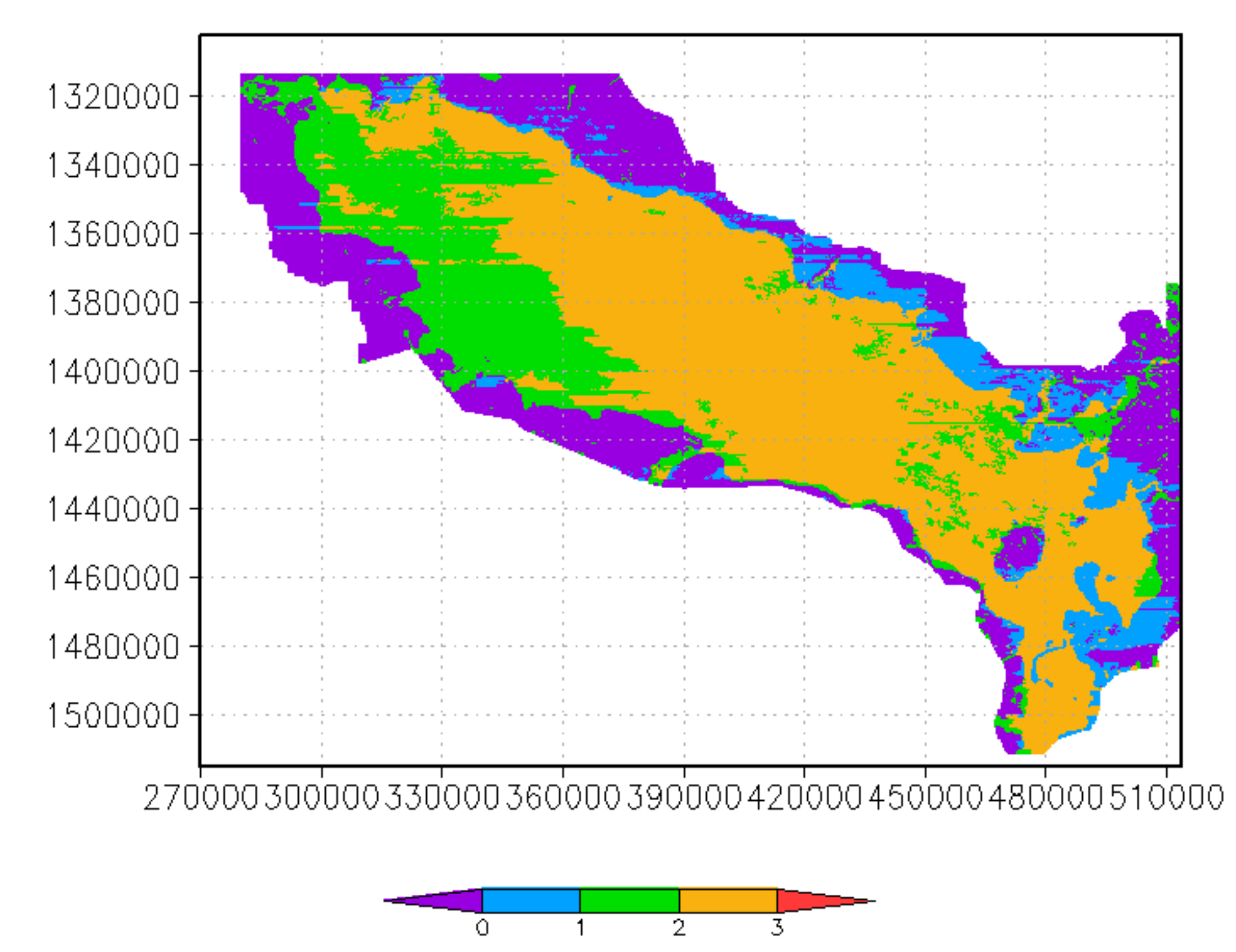
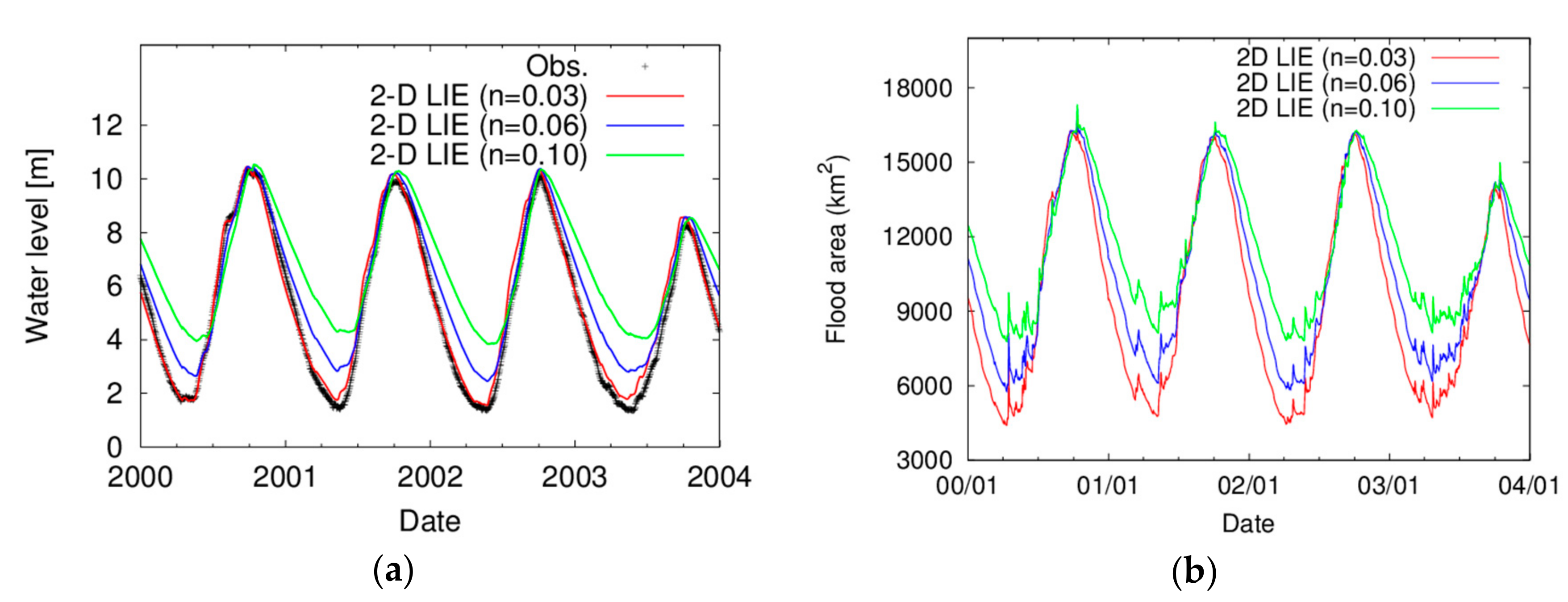
4.4. Results and Discussion
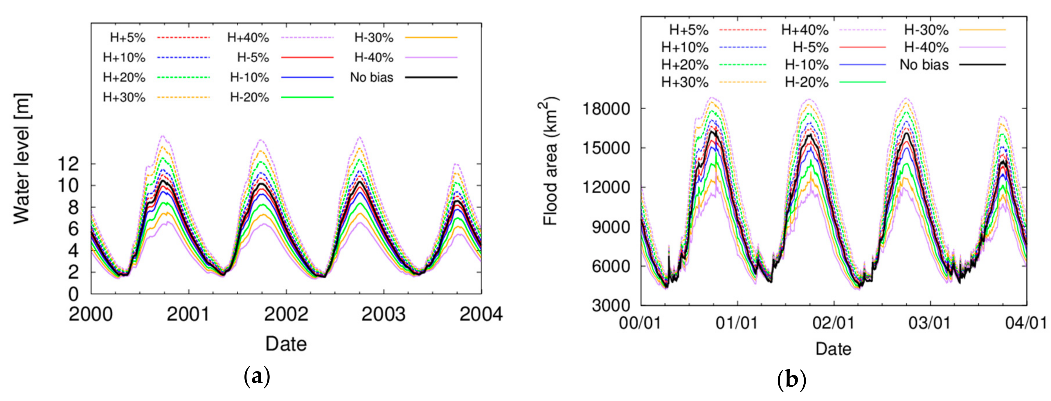
4.5. Sensitivity Analysis
5. Conclusions
Author Contributions
Funding
Acknowledgments
Conflicts of Interest
Appendix A
Appendix B
Appendix B.1. Hillslope Module
Appendix B.2. River Routing Module
References
- Alcrudo, F.; Benkhaldoun, F. Exact solutions to the Riemann problem of the shallow water equations with a bottom step. Comput. Fluids 2001, 30, 643–671. [Google Scholar] [CrossRef] [Green Version]
- Ancey, C.; Iverson, R.M.; Rentschler, M.; Denlinger, R.P. An exact solution for ideal dam-break floods on steep slopes. Water Resour. Res. 2008, 44. [Google Scholar] [CrossRef] [Green Version]
- Chesnokov, A.A. Symmetries and exact solutions of the rotating shallow-water equations. Eur. J. Appl. Math. 2009, 20, 461–477. [Google Scholar] [CrossRef]
- Thacker, W.C. Some exact solutions to the nonlinear shallow-water wave equations. J. Fluid Mech. 1981, 107, 499–508. [Google Scholar] [CrossRef]
- Miller, C.T.; Dawson, C.N.; Farthing, M.W.; Hou, T.Y.; Huang, J.; Kees, C.E.; Kelley, C.T.; Langtangen, H.P. Numerical simulation of water resources problems: Models, methods, and trends. Adv. Water Resour. 2013, 51, 405–437. [Google Scholar] [CrossRef]
- Zhang, W.; Cundy, T.W. Modeling of two-dimensional overland flow. Water Resour. Res. 1989, 25, 2019–2035. [Google Scholar] [CrossRef]
- Toro, E.F. Shock-Capturing Methods for Free-Surface Shallow Flows; John Wiley: Hoboken, NJ, USA, 2001. [Google Scholar]
- Szymkiewicz, R. Numerical Modeling in Open Channel Hydraulics; Springer Science & Business Media: Dordrecht, The Netherlands, 2010; Volume 83. [Google Scholar]
- Li, Y.; Yuan, D.; Lin, B.; Teo, F.Y. A fully coupled depth-integrated model for surface water and groundwater flows. J. Hydrol. 2016, 542, 172–184. [Google Scholar] [CrossRef]
- Şen, O.; Kahya, E. Determination of flood risk: A case study in the rainiest city of Turkey. Environ. Model. Softw. 2017, 93, 296–309. [Google Scholar] [CrossRef]
- Singh, V.P.; Woolhiser, D.A. Mathematical modeling of watershed hydrology. J. Hydrol. Eng. 2002, 7, 270–292. [Google Scholar] [CrossRef]
- Viero, D.P.; Peruzzo, P.; Carniello, L.; Defina, A. Integrated mathematical modeling of hydrological and hydrodynamic response to rainfall events in rural lowland catchments. Water Resour. Res. 2014, 50, 5941–5957. [Google Scholar] [CrossRef] [Green Version]
- Yang, X.; Chen, H.; Wang, Y.; Xu, C.Y. Evaluation of the effect of land use/cover change on flood characteristics using an integrated approach coupling land and flood analysis. Hydrol. Res. 2016, 47, 1161–1171. [Google Scholar] [CrossRef] [Green Version]
- Bates, P.D.; Horritt, M.S.; Fewtrell, T.J. A simple inertial formulation of the shallow water equations for efficient two-dimensional flood inundation modelling. J. Hydrol. 2010, 387, 33–45. [Google Scholar] [CrossRef]
- Hunter, N.M.; Bates, P.D.; Horritt, M.S.; Wilson, M.D. Simple spatially-distributed models for predicting flood inundation: A review. Geomorphology 2007, 90, 208–225. [Google Scholar] [CrossRef]
- Tanaka, T.; Yoshioka, H. Applicability of the 2-D local inertial equations to long-term hydrodynamic simulation of the Tonle Sap Lake. In Proceedings of the 2nd International Symposium on Conservation and Management of Tropical Lakes, Siem Reap, Cambodia, 24–26 August 2017. [Google Scholar]
- Almeida, G.A.; Bates, P. Applicability of the local inertial approximation of the shallow water equations to flood modeling. Water Resour. Res. 2013, 49, 4833–4844. [Google Scholar] [CrossRef] [Green Version]
- Kazezyılmaz-Alhan, C.M.; Medina, M.A., Jr. Kinematic and diffusion waves: Analytical and numerical solutions to overland and channel flow. J. Hydraul. Eng. 2007, 133, 217–228. [Google Scholar] [CrossRef]
- Liu, Q.Q.; Chen, L.; Li, J.C.; Singh, V.P. Two-dimensional kinematic wave model of overland-flow. J. Hydrol. 2004, 291, 28–41. [Google Scholar] [CrossRef] [Green Version]
- Ponce, V.M. Kinematic wave controversy. J. Hydraul. Eng. 1991, 117, 511–525. [Google Scholar] [CrossRef]
- Rudorff, C.M.; Melack, J.M.; Bates, P.D. Flooding dynamics on the lower Amazon floodplain: 1. Hydraulic controls on water elevation, inundation extent, and river-floodplain discharge. Water Resour. Res. 2014, 50, 619–634. [Google Scholar] [CrossRef] [Green Version]
- Ikeuchi, H.; Hirabayashi, Y.; Yamazaki, D.; Kiguchi, M.; Koirala, S.; Nagano, T.; Kotera, A.; Kanae, S. Modeling complex flow dynamics of fluvial floods exacerbated by sea level rise in the Ganges–Brahmaputra–Meghna Delta. Environ. Res. Lett. 2015, 10, 124011. [Google Scholar] [CrossRef]
- Apel, H.; Trepat, O.M.; Hung, N.N.; Chinh, D.T.; Merz, B.; Dung, N.V. Combined fluvial and pluvial urban flood hazard analysis: Concept development and application to Can Tho City, Mekong Delta, Vietnam. Nat. Hazards Earth Syst. 2016, 16, 941–961. [Google Scholar] [CrossRef]
- Yamazaki, D.; Sato, T.; Kanae, S.; Hirabayashi, Y.; Bates, P.D. Regional flood dynamics in a bifurcating mega delta simulated in a global river model. Geophys. Res. Lett. 2014, 41, 3127–3135. [Google Scholar] [CrossRef] [Green Version]
- Yamazaki, D.; Almeida, G.A.; Bates, P.D. Improving computational efficiency in global river models by implementing the local inertial flow equation and a vector-based river network map. Water Resour. Res. 2013, 49, 7221–7235. [Google Scholar] [CrossRef] [Green Version]
- Ikeuchi, H.; Hirabayashi, Y.; Yamazaki, D.; Muis, S.; Ward, P.J.; Winsemius, H.C.; Verlaan, M.; Kanae, S. Compound simulation of fluvial floods and storm surges in a global coupled river-coast flood model: Model development and its application to 2007 Cyclone Sidr in Bangladesh. J. Adv. Model. Earth Syst. 2017, 9, 1847–1862. [Google Scholar] [CrossRef]
- Coles, D.; Yu, D.; Wilby, R.L.; Green, D.; Herring, Z. Beyond ‘flood hotspots’: Modelling emergency service accessibility during flooding in York, UK. J. Hydrol. 2017, 546, 419–436. [Google Scholar] [CrossRef]
- Dottori, F.; Todini, E. Testing a simple 2D hydraulic model in an urban flood experiment. Hydrol. Process. 2013, 27, 1301–1320. [Google Scholar] [CrossRef]
- Falter, D.; Vorogushyn, S.; Lhomme, J.; Apel, H.; Gouldby, B.; Merz, B. Hydraulic model evaluation for large-scale flood risk assessments. Hydrol. Process. 2013, 27, 1331–1340. [Google Scholar] [CrossRef]
- Yin, J.; Yu, D.; Wilby, R. Modelling the impact of land subsidence on urban pluvial flooding: A case study of downtown Shanghai, China. Sci. Total Environ. 2016, 544, 744–753. [Google Scholar] [CrossRef] [PubMed] [Green Version]
- Yin, J.; Yu, D.; Yin, Z.; Liu, M.; He, Q. Evaluating the impact and risk of pluvial flash flood on intra-urban road network: A case study in the city center of Shanghai, China. J. Hydrol. 2016, 537, 138–145. [Google Scholar] [CrossRef] [Green Version]
- Zellou, B.; Rahali, H. Assessment of reduced-complexity landscape evolution model suitability to adequately simulate flood events in complex flow conditions. Nat. Hazards 2017, 86, 1–29. [Google Scholar] [CrossRef]
- Pontes, P.R.M.; Fan, F.M.; Fleischmann, A.S.; de Paiva, R.C.D.; Buarque, D.C.; Siqueira, V.A.; Jardim, P.F.; Sorribas, M.V.; Collischonn, W. MGB-IPH model for hydrological and hydraulic simulation of large floodplain river systems coupled with open source GIS. Environ. Model. Softw. 2017, 94, 1–20. [Google Scholar] [CrossRef]
- Martins, R.; Leandro, J.; Djordjević, S. A well balanced Roe scheme for the local inertial equations with an unstructured mesh. Adv. Water Resour. 2015, 83, 351–363. [Google Scholar] [CrossRef]
- Martins, R.; Leandro, J.; Djordjević, S. Analytical and numerical solutions of the Local Inertial Equations. Int. J. Non-Linear Mech. 2016, 81, 222–229. [Google Scholar] [CrossRef] [Green Version]
- Martins, R.; Leandro, J.; Djordjević, S. Wetting and drying numerical treatments for the Roe Riemann scheme. J. Hydraul. Res. 2017, in press. [Google Scholar] [CrossRef]
- Carbonnel, J.P.; Guiscafre, J. Ministiere des Affaires Etrangeres. Gouvernement Royal du Cambodge Grand Lac du Cambodge; Muséum National D’histoire Naturelle de Paris: Paris, France, 1962; 63p. [Google Scholar]
- Lamberts, D. The Tonle Sap Lake as a productive ecosystem. Int. J. Water Resour. Dev. 2006, 22, 481–495. [Google Scholar] [CrossRef]
- Uk, S.; Yoshimura, C.; Siev, S.; Try, S.; Yang, H.; Oeurng, C.; Li, S.; Hul, S. Tonle Sap Lake: Current status and important research directions for environmental management. Lakes Reserv. Res. Manag. 2018, in press. [Google Scholar] [CrossRef]
- Ahamed, A.; Bolten, J.D. A MODIS-based automated flood monitoring system for southeast Asia. Int. J. Appl. Earth Obs. Geoinf. 2017, 61, 104–117. [Google Scholar] [CrossRef]
- Hai, P.T.; Masumoto, T.; Shimizu, K. Development of a two-dimensional finite element model for inundation processes in the Tonle Sap and its environs. Hydrol. Process. 2008, 22, 1329–1336. [Google Scholar] [CrossRef]
- Masumoto, T.; Hai, P.T.; Shimizu, K. Impact of paddy irrigation levels on floods and water use in the Mekong River basin. Hydrol. Process. 2008, 22, 1321–1328. [Google Scholar] [CrossRef]
- Tangdamrongsub, N.; Ditmar, P.G.; Steele-Dunne, S.C.; Gunter, B.C.; Sutanudjaja, E.H. Assessing total water storage and identifying flood events over Tonlé Sap basin in Cambodia using GRACE and MODIS satellite observations combined with hydrological models. Remote Sens. Environ. 2016, 181, 162–173. [Google Scholar] [CrossRef]
- Hung, N.N.; Delgado, J.M.; Güntner, A.; Merz, B.; Bárdossy, A.; Apel, H. Sedimentation in the floodplains of the Mekong Delta, Vietnam. Part I: Suspended sediment dynamics. Hydrol. Process. 2014, 28, 3132–3144. [Google Scholar] [CrossRef]
- Kabeya, N.; Kubota, T.; Shimizu, A.; Nobuhiro, T.; Tsuboyama, Y.; Chann, S.; Tith, N. Isotopic investigation of river water mixing around the confluence of the Tonle Sap and Mekong rivers. Hydrol. Process. 2008, 22, 1351–1358. [Google Scholar] [CrossRef]
- Västilä, K.; Kummu, M.; Sangmanee, C.; Chinvanno, S. Modelling climate change impacts on the flood pulse in the Lower Mekong floodplains. J. Water Clim. Chang. 2010, 1, 67–86. [Google Scholar] [CrossRef]
- Yang, D.; Oki, T.; Herath, S.; Musiake, K. A hillslope-based hydrological model using catchment area and width functions. Hydrol. Sci. J. 2002, 47, 49–65. [Google Scholar] [CrossRef] [Green Version]
- Fujii, H.; Garsdal, H.; Ward, P.; Ishii, M.; Morishita, K.; Boivin, T. Hydrological roles of the Cambodian floodplain of the Mekong River. Int. J. River Basin Manag. 2003, 1, 253–266. [Google Scholar] [CrossRef]
- Cong, Z.; Yang, D.; Gao, B.; Yang, H.; Hu, H. Hydrological trend analysis in the Yellow River basin using a distributed hydrological model. Water Resour. Res. 2009, 45. [Google Scholar] [CrossRef] [Green Version]
- Wang, W.; Lu, H.; Yang, D.; Sothea, K.; Jiao, Y.; Gao, B.; Peng, X.; Pang, Z. Modelling hydrologic processes in the Mekong River Basin using a distributed model driven by satellite precipitation and rain gauge observations. PLoS ONE 2016, 11, e0152229. [Google Scholar] [CrossRef] [PubMed]
- Verdin, K.L.; Verdin, J.P. A topological system for delineation and codification of the Earth’s river basins. J. Hydrol. 1999, 218, 1–12. [Google Scholar] [CrossRef]
- Rauch, W.; Bertrand-Krajewski, J.L.; Krebs, P.; Mark, O.; Schilling, W.; Schütze, M.; Vanrolleghem, P.A. Deterministic modelling of integrated urban drainage systems. Water Sci. Technol. 2002, 45, 81–94. [Google Scholar] [CrossRef] [PubMed]
- Kourgialas, N.N.; Karatzas, G.P. A hydro-sedimentary modeling system for flash flood propagation and hazard estimation under different agricultural practices. Nat. Hazards Earth Syst. 2014, 14, 625–634. [Google Scholar] [CrossRef] [Green Version]
- Li, Q.; Wang, T.; Zhu, Z.; Meng, J.; Wang, P.; Suriyanarayanan, S.; Zang, Y.; Song, S.; Lu, Y.; Yvette, B. Using hydrodynamic model to predict PFOS and PFOA transport in the Daling River and its tributary, a heavily polluted river into the Bohai Sea, China. Chemosphere 2017, 167, 344–352. [Google Scholar] [CrossRef] [PubMed]
- Doulgeris, C.; Georgiou, P.; Papadimos, D.; Papamichail, D. Ecosystem approach to water resources management using the MIKE 11 modeling system in the Strymonas River and Lake Kerkini. J. Environ. Manag. 2012, 94, 132–143. [Google Scholar] [CrossRef] [PubMed]
- Abbot, M.B.; Ionescu, F. On the numerical computation of nearly-horizontal flows. J. Hydraul. Res. 1967, 5, 97–117. [Google Scholar] [CrossRef]
- Yoshioka, H.; Tanaka, T. On mathematics of the 2-D local inertial model for flood simulation. In Proceedings of the 2nd International Symposium on Conservation and Management of Tropical Lakes, Siem Reap, Cambodia, 24–26 August 2017. [Google Scholar]
- Yoshioka, H.; Tanaka, T. Numerical stability analysis of the local inertial equation with semi- and fully-implicit friction term treatments. J. Adv. Simul. Sci. Eng. 2018, 4, 162–175. [Google Scholar]
- Sakamoto, T.; Nguyen, N.V.; Kotera, A.; Ohno, H.; Ishitsuka, N.; Yokozawa, M. Detecting temporal change in the extent of annual flooding within the Cambodia and the Vietnamese Mekong Delta from MODIS time-series imagery. Remote Sens. Environ. 2007, 109, 295–313. [Google Scholar] [CrossRef]
- Sakamoto, T.; Van, P.C.; Kotera, A.; Duy, K.N.; Yokozawa, M. Detection of yearly change in farming systems in the Vietnamese Mekong Delta from MODIS time-series imagery. Jpn. Agric. Res. Q. 2009, 43, 173–185. [Google Scholar] [CrossRef]
- FAO. The Digital Soil Map of the World and Derived Soil Properties, version 3.6; FAO/UNESCO: Rome, Italy, 2003. [Google Scholar]
- MRC. Consolidation of Hydro-Meteorological Data and Multi-Functional Hydrologic Roles of Tonle Sap Lake and its Vicinity Project; Main Report Chapter 9; Mekong River Commission: Phnom Penh, Cambodia, 2003; pp. 1–18. [Google Scholar]
- MRC. The Study on Hydro-Meteorological Monitoring for Water Quantity Rules in the Mekong River Basin; Final Report; Mekong River Commission: Phnom Penh, Cambodia, 2004; Volume 1, Part III; pp. 1–68. [Google Scholar]
- Kummu, M.; Tes, S.; Yin, S.; Adamson, P.; Jozsa, J.; Koponen, J.; Richey, J.; Sarkkula, J. Water balance analysis for the Tonle Sap Lake–floodplain system. Hydrol. Process. 2014, 28, 1722–1733. [Google Scholar] [CrossRef]
- Ministry of Public Works and Transport, Cambodia. JICA Map of Cambodia. 1:100,000; Ministry of Public Works and Transport, Cambodia: Phnom Penh, Cambodia, 1997.
- Kummu, M.; Penny, D.; Sarkkula, J.; Koponen, J. Sediment: Curse or blessing for Tonle Sap Lake? Ambio J. Hum. Environ. 2008, 37, 158–163. [Google Scholar] [CrossRef]
- Lu, X.; Kummu, M.; Oeurng, C. Reappraisal of sediment dynamics in the Lower Mekong River, Cambodia. Earth Surf. Process. Landf. 2014, 39, 1855–1865. [Google Scholar] [CrossRef]
- Schmitt, R.J.P.; Rubin, Z.; Kondolf, G.M. Losing ground-scenarios of land loss as consequence of shifting sediment budgets in the Mekong Delta. Geomorphology 2017, 294, 58–69. [Google Scholar] [CrossRef]
- Siev, S.; Yang, H.; Sok, T.; Uk, S.; Song, L.; Kodikara, D.; Oeurng, C.; Hul, S.; Yoshimura, C. Sediment dynamics in a large shallow lake characterized by seasonal flood pulse in Southeast Asia. Sci. Total Environ. 2018, 631–632, 597–607. [Google Scholar] [CrossRef] [PubMed]
- Thanh, V.Q.; Reyns, J.; Wackerman, C.; Eidam, E.F.; Roelvink, D. Modelling suspended sediment dynamics on the subaqueous delta of the Mekong River. Cont. Shelf Res. 2017, 147, 213–230. [Google Scholar] [CrossRef]
- Kc, K.; Bond, N.; Fraser, E.D.G.; Elliott, V.; Farrell, T.; McCann, K.; Rooney, N.; Bieg, C. Exploring tropical fisheries through fishers’ perceptions: Fishing down the food web in the Tonlé Sap, Cambodia. Fish. Manag. Ecol. 2017, 24, 452–459. [Google Scholar] [CrossRef]
- Kong, H.; Chevalier, M.; Laffaille, P.; Lek, S. Spatio-temporal variation of fish taxonomic composition in a South-East Asian flood-pulse system. PLoS ONE 2017, 12, e0174582. [Google Scholar] [CrossRef] [PubMed]
- Sogreah. Mathematical Model of Mekong Delta. Comprehensive Report of the Different Determinations on the Grand Lac Capacity; Sogreah: Phnom Penh, Cambodia, 1999. [Google Scholar]


| Simulation Condition | |||
| Gradient [-] | 0.001 | 0.005 | 0.01 |
| Water depth [m] | 0.1 | 1.0 | 2.0 |
| Maximum Allowable Time Step [s] | |||
| CFL condition | 505 | 150 | 113 |
| Explicit treatment | 23.1 | 38.8 | 23.9 |
| Semi-implicit treatment | 152 | 63.9 | 45.2 |
© 2018 by the authors. Licensee MDPI, Basel, Switzerland. This article is an open access article distributed under the terms and conditions of the Creative Commons Attribution (CC BY) license (http://creativecommons.org/licenses/by/4.0/).
Share and Cite
Tanaka, T.; Yoshioka, H.; Siev, S.; Fujii, H.; Fujihara, Y.; Hoshikawa, K.; Ly, S.; Yoshimura, C. An Integrated Hydrological-Hydraulic Model for Simulating Surface Water Flows of a Shallow Lake Surrounded by Large Floodplains. Water 2018, 10, 1213. https://doi.org/10.3390/w10091213
Tanaka T, Yoshioka H, Siev S, Fujii H, Fujihara Y, Hoshikawa K, Ly S, Yoshimura C. An Integrated Hydrological-Hydraulic Model for Simulating Surface Water Flows of a Shallow Lake Surrounded by Large Floodplains. Water. 2018; 10(9):1213. https://doi.org/10.3390/w10091213
Chicago/Turabian StyleTanaka, Tomohiro, Hidekazu Yoshioka, Sokly Siev, Hideto Fujii, Yoichi Fujihara, Keisuke Hoshikawa, Sarann Ly, and Chihiro Yoshimura. 2018. "An Integrated Hydrological-Hydraulic Model for Simulating Surface Water Flows of a Shallow Lake Surrounded by Large Floodplains" Water 10, no. 9: 1213. https://doi.org/10.3390/w10091213