Engineering Analysis of Plant and Fungal Contributions to Bioretention Performance
by
Alex Taylor
1,2, 
Jill Wetzel
3,
Emma Mudrock
3,
Kennith King
4,
James Cameron
5,
Jay Davis
4 and
Jenifer McIntyre
3,* 1
Department of Biological Systems Engineering, Puyallup Research & Extension Center, Washington State University, Puyallup, WA 98371, USA
2
Fungi Perfecti, LLC, Olympia, WA 98507, USA
3
School of the Environment, Puyallup Research & Extension Center, Washington State University, Puyallup, WA 98371, USA
4
U.S. Fish & Wildlife Service, Washington Fish & Wildlife Office, Lacey, WA 98503, USA
5
Earth Resources Technologies, under Contract to NOAA, National Marine Fisheries Service, Northwest Fisheries Science Center, Environmental and Fisheries Science Division, Seattle, WA 98112, USA
*
Author to whom correspondence should be addressed.
Water 2018, 10(9), 1226; https://doi.org/10.3390/w10091226
Submission received: 13 July 2018
/
Revised: 6 September 2018
/
Accepted: 8 September 2018
/
Published: 12 September 2018
(This article belongs to the Special Issue Plant and Microbial Processes in Stormwater Treatment Systems)
Abstract
:While the use of bioretention for stormwater management is widespread, data about the impacts of plants and microorganisms on long-term treatment efficacy remain region-specific. To help address this knowledge gap for the Pacific Northwest region of the United States, we installed twelve under-drained bioretention mesocosms built to Washington State Department of Ecology stormwater management standards in an urban watershed in Seattle, WA that included a busy portion of Interstate 5. Six mesocosms were planted with Pacific ninebark (Physocarpus capitatus) and six were inoculated with the wine cap mushroom (Stropharia rugoso-annulata) resulting in four replicated factorial treatments. Because region-specific studies must be mindful of the prevailing regulatory framework, all mesocosms used the Washington State Department of Ecology design standard soil: a blend of 60% sand and 40% compost by volume, despite the known leaching problems with high compost volume fraction soils. Five water quality sampling events over 15 months of continuous stormwater loading were analyzed for dozens of water quality parameters. Multiple linear regression analyses of treatment differences over the 400-day loading period illustrate that incorporating fungi into the wood mulch slowed the release of total and ortho-phosphorus from the bioretention soil; however net export of phosphorus from this compost rich media continued through 400 days of loading for all treatments. Multivariate ordination methods illustrate that time and temperature dramatically affect performance of this media, but the impact of planting and fungal inoculation had marginal detectible effects on overall water quality during the study timeframe. These results demonstrate that future studies of this media blend must plan for at least one year of nutrient and metal leaching before the time-dependent heterogenous variance introduced by these exports will no longer pose an obstacle to analysis of other performance changing factors. The results highlight important physical and chemical considerations for this media blend, and the opportunity for continued research on the use of fungal inoculated mulch application as a new ecological engineering tool for reducing phosphorus leaching from soils.
Keywords:
bioretention; stormwater; fungi; mycelium; plants; compost; water quality; nutrients; rain gardens; green infrastructure; mushroom
1. Introduction
The many deleterious effects of urban stormwater runoff on US surface waters have been extensively described for over a decade [1]. While bioretention has demonstrated unequivocal improvements in stormwater management when compared with historical “grey infrastructure” questions about how to implement it most effectively have been under investigation for over a decade and remains an area of active research [2,3].
The ambiguity about how to best implement bioretention is particularly evident in the debate around bioretention soil composition and the search for improved formulations [4,5]. Bioretention soil as a global stormwater BMP is far from a universally consistent formulation. Most municipalities use different mixes including some combination of sand, native soil, organic matter such as compost or bark, and sometimes additional amendments such as wastewater treatment residuals, biochar, iron-containing sands, fly ash, etc. [6]. All bioretention soils are intended to provide high infiltration rates, water holding capacity, specific surface area, and cation exchange.
The bioretention soil mix (BSM) used in this study was the default mixture codified by the 2014 Washington State Department of Ecology Stormwater Management Manual for Western Washington (SWMMWW): a mixture of 60% sand and 40% compost v/v [7]. Previous studies in Washington State with this BSM have documented significant exports of biological oxygen demand, nitrogen, and phosphorus both in the laboratory [8] and in the field [3,9]. Those results are echoed in a 2014 study published by American Society of Civil Engineers that found increasing compost volume fraction is correlated with decreasing hydraulic conductivity and increasing phosphorus export [10]. Despite these detriments, the use of this mixture continues to be defended by Washington State [11], citing, for example, demonstrated substantial reductions in sediment, hydrocarbons, zinc, and bacteria [3], and elimination of the otherwise acute toxicity of urban runoff to coho salmon [12,13].
In addition to the soil composition of BSM, there is considerable interest in the role of plants and how the plant palette can be regionally optimized for water quality and pollutant retention design goals. A number of studies have demonstrated water quality improvements in planted systems, which have been recently reviewed [2,6], while other studies on nutrient removal have been unable to document any significant difference in effluent water quality between planted and unplanted bioretention soil [14]. An additional difficulty lies in the different physical and physiological attributes of the plants used in bioretention. A 2012 study of the effect of plants on bioretention soil hydraulic conductivity found that thick-rooted plants helped maintain or improve hydraulic conductivity, while plants with finer roots tended to form a root mat that decreased hydraulic conductivity [15].
Recently there has also been discussion among environmental engineers about the role of microorganisms, particularly fungi, in bioretention performance. Several bench and field-scale studies suggest that wood-decomposing fungi can be used in bioretention mulch to provide unique environmental services. A 2009 field study of two under-drained rain gardens in Washington State found that inoculating the wood mulch layer with saprophytic fungi removed 24% more faecal coliform from runoff than the control [16]. A 2014 laboratory study found that the mushroom-forming fungus Stropharia rugoso-annulata grown on alder wood chips yielded a 20% improvement in E. coli removal relative to the wood chips alone at the hydraulic loading rate of 0.43 m3/m2·d [17]. Importantly, the research also indicated that S. rugoso-annulata is robust to environmental stresses (saturation, dehydration, and temperature fluctuations from −20 °C to 40 °C). S. rugoso-annulata and other saprophytic macrofungi can also degrade recalcitrant PAHs in contaminated soil, with reductions of 70–80% for benzo(a)anthracene, benzo(a)pyrene, and dibenzo(a,h)anthracene [18]. Numerous additional studies have documented that fungi can similarly degrade other recalcitrant xenobiotic toxicants such as insecticides [19].
The study reported here was designed to test the reproducibility of fungal and plant mediated effects on the quality of stormwater in replicated bioretention systems operating under field conditions for an extended period of time. To assure applicability of the study to Washington State watershed management decisions regulated by the Clean Water Act, the bioretention systems were installed according to Washington State Department of Ecology specifications [7]. To assure that potentially small differences between mesocosms could be detected through variance introduced by heterogenous soil preparation and installation, these parameters were defined in the laboratory and controlled in the field.
2. Materials and Methods
2.1. Calibrating Bioretention Soil Composition
Two cubic meters of mature compost from municipal yard and food waste feedstock and two cubic meters of sand were donated by Cedar Grove Composting, Inc. (Maple Valley, WA, USA) in August 2016. Each of these materials met SWMMWW specifications for particle size gradation, organic matter, and nutrients, among other QA parameters (Supplementary materials). Prior to mixing the sand and compost into BSM, representative composite samples of each were collected and analyzed for total and dissolved metals by method SW-846 6020A (AmTest Laboratories; Kirkland, WA, USA). Compost was additionally sent to SoilTest Farm Consultants, Inc. (Moses Lake, WA, USA) for analysis of total nitrogen (ASTM D5373), total carbon (ASTM D5373), nitrate (S-3.10 b), ammonia (S-3.50), total phosphorus (EPA 3050A/6010B), Olsen phosphorus (S-4.20 b), cation exchange capacity (S-10.10 b), and pH.
To achieve a well-mixed BSM, small batches (25 L) were individually prepared for filling the field mesocosms. Each batch was proportioned by un-compacted volume of sand (15 L) and compost (10 L), collected from a composite of samples that were randomly collected from different locations in the sand or compost pile. Compost was sifted through a 1.3 cm screen (100% passing) to break up clods and achieve a relatively even compost density prior to volumetric proportioning. Sand and compost were proportioned by volume and the wet weight for each portion was recorded. A composite sub-sample was collected from each 25-L BSM batch for moisture analysis so that the total dry mass of each BSM batch could be estimated [20]. Additional moisture samples of the sand and compost were collected between every fifth batch to allow estimation of the total dry mass of sand and compost within each 25-L batch.
2.2. Calibrating BSM Installation Parameters
2.2.1. Bulk Density
Washington State regulations state that BSM should be installed at a bulk density that corresponds to 85% of the modified maximum dry density. This value was determined from a plot of moisture content versus bulk density under uniform compaction as described in ASTM 1557 [21].
2.2.2. Saturated Hydraulic Conductivity
Samples of BSM were compacted with variable force to produce seven columns with a range of soil bulk densities. The saturated hydraulic conductivity of each column was determined by the falling head method [22].
2.2.3. Soil Moisture Characteristic
The soil moisture characteristic of BSM at three bulk densities was determined using the hanging water column method with supplementary higher suction data points collected using the pressure plate method at 0.3 bar and 1.0 bar of pressure [22].
2.3. Installation of Mesocosms
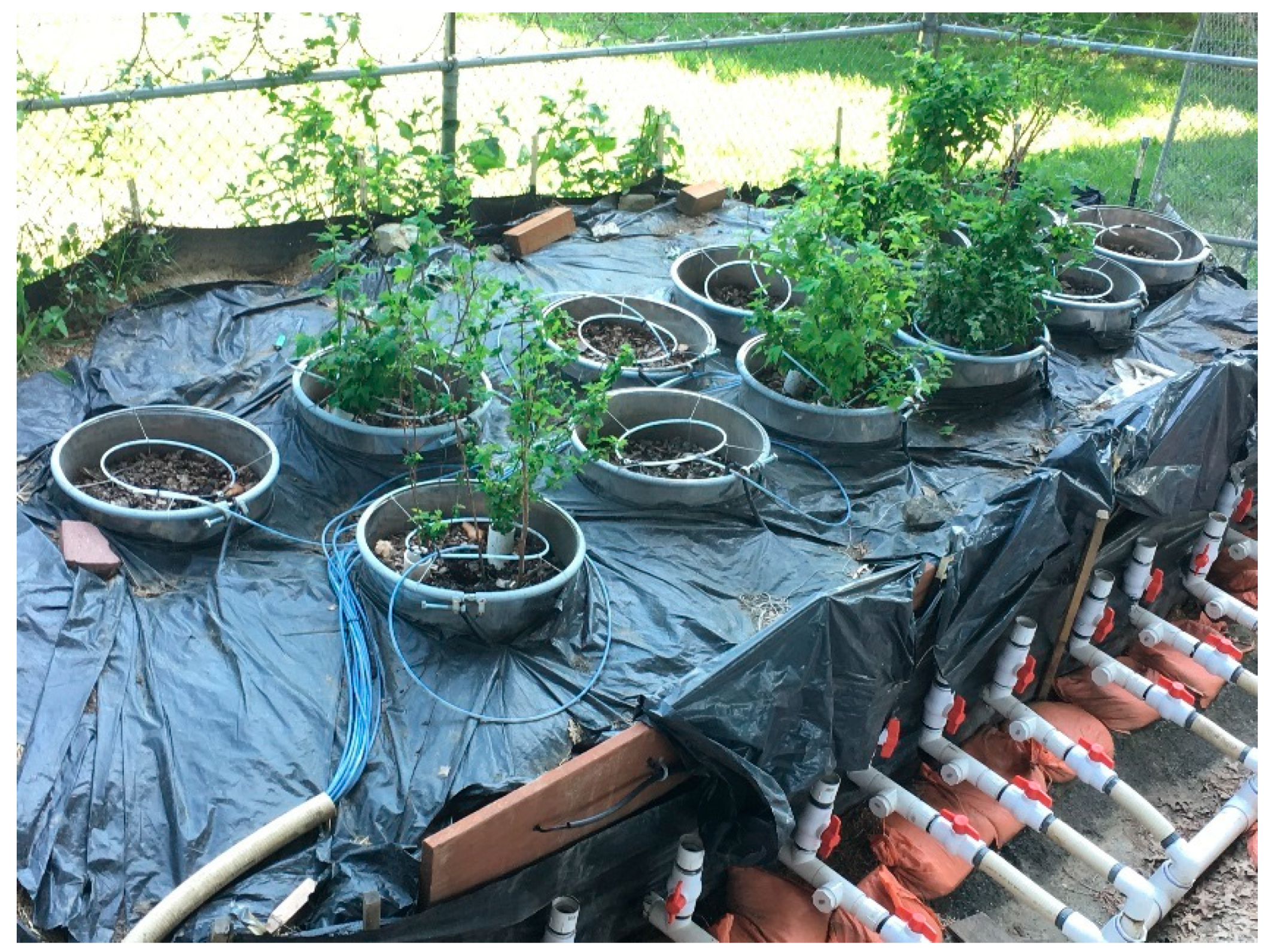
Twelve bioretention mesocosms were installed at the Washington State Department of Transportation Lake Union ship canal research facility, located at 648 NE 40th St., Seattle WA (Figure 1). The site receives runoff from a 12.8-hectare drainage area including 9.2 hectares of pavement and 3.6 hectares of roadside landscaping. The majority of the pavement in the site’s watershed is the I-5 roadway—the busiest section of roadway in Washington state with a 2017 average annual daily traffic volume of 208,000 vehicles per day [23].
Bioretention mesocosms (217 L each) were built in 304-stainless steel drums (57.15 cm diameter, 84.77 mm height, 1.6 mm thick) acquired from Skolnik Industries, Inc. (Chicago, IL, USA). Each drum was fitted with a 5-cm diameter slotted underdrain made from commercial well casing pipe (Denver Winpump Company, Denver, CO, USA). The drain pipe was imbedded in a layer of City of Seattle type 26 drain aggregate such that the gravel drainage layer extended 15.2 cm above the crown of the pipe, with the trough of the pipe 3.8 cm above the bottom of the drum. The total gravel drainage layer depth was 24 cm. The BSM was added to each drum based on total dry mass (145 ± 2.8 kg) and was compacted to a target depth of 40.1 ± 1.0 cm to achieve the target bulk density of 1.41 ± 0.04 g cm−3.
To improve the thermal stability of the mesocosm installation, a retaining structure was built around the 12 mesocosms and filled with approximately 20 m3 of clay loam to a depth of approximately 70 cm with a 30–60 cm wide perimeter between the mesocosms and the retaining structure. The fill surrounding each drum was mulched with straw and covered with black plastic sheeting to prevent erosion or sediment movement from the fill into the mesocosms.
Six of the twelve mesocosms were planted with Pacific ninebark (Physocarpus capitatus) purchased in 4 L pots from Woodbrook Native Plant Nursery (Gig Harbor, WA, USA). Prior to installation each plant was removed from its pot and thoroughly rinsed to remove potting soil and slow release fertilizer pellets. The total bare-root plant mass was recorded for each plant. Each planted mesocosm received three small (130 ± 90 g) bareroot transplants for a total of 400 ± 50 g of Pacific ninebark per mesocosm.
All twelve bioretention mesocosms received a three-inch layer of alder (Alnus rubra) mulch (60% wood chips, 40% coarse sawdust by volume). Mulch was distributed by wet mass (10.0 ± 0.4 kg per bioretention cell). Six of the mesocosms were inoculated with mycelium of the wine cap mushroom (Stropharia rugoso-annulata) donated by Fungi Perfecti, LLC (Olympia, WA, USA). Inoculated mesocosms received 6.6 ± 0.3 kg of mycelium-infused alder mulch plus 3.4 ± 0.1 kg of alder mulch without fungal mycelium, while uninoculated mesocosms received 10.0 ± 0.4 kg of alder mulch without fungal mycelium.
Every mesocosm was equipped with probes (METER Group, Inc., Pullman, WA, USA) to measure soil moisture, temperature, and electrical conductivity (model 5TE); soil matric potential (model MPS6), and corresponding digital data loggers (model EM50). Soil probes were placed in the center area of each drum after 50% of the soil mass had been added (20 ± 5 cm below the soil surface).
The baseline saturated hydraulic conductivity (Ksat) of the operational field mesocosms was determined using the falling head method [22]. For each field saturated hydraulic conductivity test, a peristaltic pump was used to transfer municipal water into a stand pipe affixed in the drain of each mesocosm at a rate of 0.4 L min−1, followed by 24–72 h of saturation. Each mesocosm was tested multiple times.
2.4. Mesocosm Hydraulic Loading Parameters
The bioretention system was in continuous operation over a 400-day period. Stormwater was distributed at a constant rate of 0.12 L min−1 to each mesocosm from a catch basin vault fitted with a float switch that activated a 12-channel peristaltic pumping system comprised of two MasterFlex L/S 100 RPM peristaltic pumps, each equipped with a three roller six channel pump head. During storm events, the pumps would activate and draw stormwater through a 15 m long, 11 mm diameter PTFE tube into a PTFE manifold with 12 individual outlets for each of the 12 peristaltic pump channels.
A data-logging Dynasonics DFX doppler ultrasonic flow meter (Badger Meter, Milwaukee, WI, USA) recorded stormwater flow rates at 1-min intervals when the pumps were operating. These 1-min pumping rates were integrated over time to calculate the total runoff volume treated-to-date by each mesocosm. Platinum-cured silicone peristaltic pump tubing in each channel delivered 12 individual aliquots of the stormwater through individual 5-m long, 5.5 mm diameter PTFE tubing to each mesocosm. The pumping rate was calculated based on a 6-month design storm for the city of Seattle (3.3 cm over 24 h) for a 20:1 contributing area to treatment area ratio. This yielded a stormwater influent flow rate of 0.12 L min−1 into each mesocosm.
2.5. Mesocosm Stormwater Sampling
Influent and effluent stormwater was monitored during five quarterly sampling events over a 400-day period beginning 15 February 2017. For each sampling event, effluent samples were collected from each of the 12 bioretention mesocosms and were compared with composite influent samples. Influent samples were collected in acid washed 4-L amber glass bottles placed next to each mesocosm. At the beginning of each sampling event, the 12 influent bottles were filled for five minutes each such that each influent bottle received approximately 0.6 L of influent. The influent water from each mesocosm was then added into one of three acid washed 20-L carboys stored on ice. Each of the influent carboys received the composited influent water from four randomly selected mesocosms. In this way, influent composite samples were taken in triplicate, with each replicate representing the average influent to four randomly selected mesocosms.
After five minutes the influent water was again directed into the bioretention mesocosms, and effluent sample collection began. Effluent water from each mesocosm was collected in acid washed 500 mL wide-mouth glass bottles, which were used to transport the water into one of 12 acid washed 20-L carboys stored on ice. This 20-min collection resulted in approximately 2.4 L of effluent that was added to each of the effluent carboys. This entire process (influent and effluent collection) was repeated three times so that samples of influent and effluent were collected contemporaneously over approximately the 1.25 h required to collect the necessary volume for chemical analysis.
After sample collection, a clean Teflon magnetic stir bar was added to each 20-L carboy. Carboys were placed onto magnetic stir plates and sampling caps were installed. Each sampling cap was a high-density foam with an acid washed borosilicate glass rod protruding through and an additional hole in the foam cork to receive a positive pressure air line. An air pump was used to positively pressurize each carboy in order to force the continuously stirring stormwater up through the tube for water quality aliquot collection. All water quality aliquots were stored at 4 °C. Water samples for PAH analysis were field extracted in 10% analysis-grade methylene chloride to prevent degradation prior to analysis.
Water samples were analyzed for Fecal Coliform (SM 9222D), E. coli (SM 9221F1), pH (SM 4500H B), Total Suspended Solids (SM 2540D), Biological Oxygen Demand (SM 5210B), Total Organic Carbon (SM 5310B), Dissolved Organic Carbon (SM 5310B), Alkalinity (SM 2320B), Ammonia/Ammonium (EPA 350.1), Total Nitrogen (EPA 351.2), Nitrate/Nitrite (EPA 353.2), Ortho-Phosphate (SM 4500-P E), Total Phosphorus (SM 4500-P F), Total and Dissolved Metals (EPA 200.8), and 18 PAH congeners (EPA 8270D-SIM).
2.6. Statistical Analyses
Data organization, exploration, and analysis were conducted using the statistical computing language R (version 3.4.0) implemented in the RStudio (version 1.0.143) software environment [24,25]. Most data handling was conducted using the base package, with additional functions from the dplyr package (version 0.7.5) used in the reorganization of the raw data [26]. Statistical analysis was implemented using the R ‘stats’ package (version 3.4.0), ‘car’ (version 3.0-0) [27], ‘MVN’ (version 5.1) [28], ‘psych’ (version 1.8.4) [29], and ‘vegan’ (version 2.5-2) [30].
3. Results
3.1. Calibrating Bioretention Soil Composition
Based on the measured gravimetric moisture content of the BSM during preparation, the calculated dry-mass composition of each batch was 86 ± 4% sand and 14 ± 1% compost. This data was used to standardize the BSM in each of twelve field bioretention cells by a calculated estimate of total dry mass.
To ascertain the relative contributions of sand and compost to the metals content of the BSM, representative samples of each media component were analyzed in triplicate for a suite of total and dissolved metals (Table 1). These data illustrate that the compost generally contained more metals by dry mass than the sand—particularly for copper, zinc, and lead. However, the BSM metal concentrations are more similar to the sand due to the high sand composition.
The nutrient concentration, cation exchange capacity, and pH was measured on the mixed BSM directly (Table 2). The results illustrate that the soil composition is within the typical ranges for this media composition reported in the literature [6]. It is notable that plant available phosphorus, as estimated using the Olsen method, is a concentration that would be considered “low” from an agronomic perspective [31].
3.2. Calibrating BSM Installation Parameters
3.2.1. Bulk Density and Saturated Hydraulic Conductivity
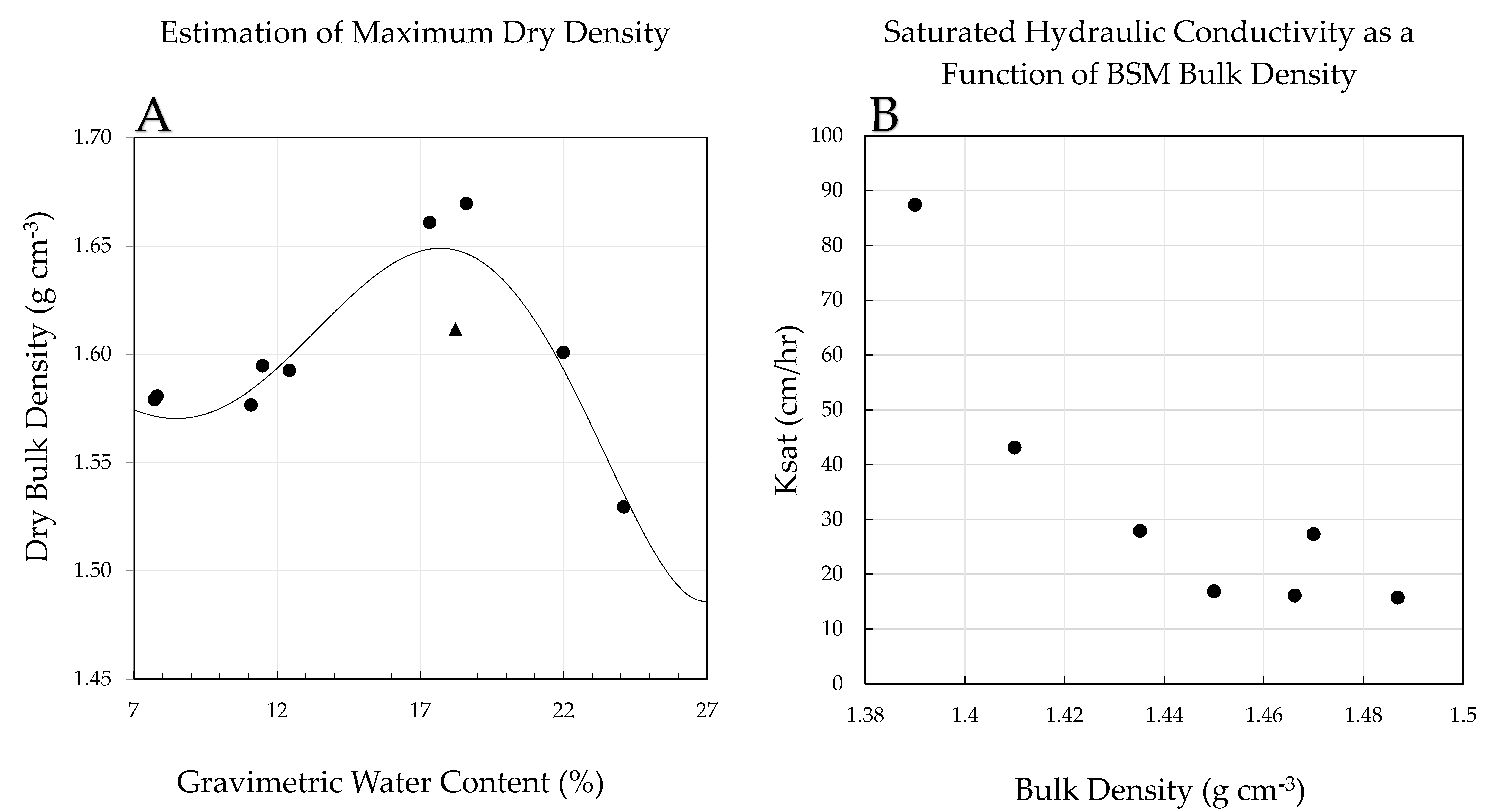
In order to ensure that the study met the SWMMWW specifications, the target soil bulk density and the corresponding saturated hydraulic conductivity were determined experimentally. The general trend in Figure 2A follows the anticipated curvilinear response described in the ASTM method referenced by the SWMMWW. These data indicate a maximum dry density of roughly 1.65 g cm−3 giving a target installation bulk density of 1.40 g cm−3. The BSM Ksat decreased as a predictable function of bulk density (Figure 2B). The BSM demonstrated the target saturated hydraulic conductivity (30 cm h−1) at approximately 1.44 g cm−3 or 87% of the maximum dry density. These may also be useful baseline reference data for future studies or bioretention installations in Washington state that utilize this BSM formulation.
3.2.2. Soil Moisture Characteristic
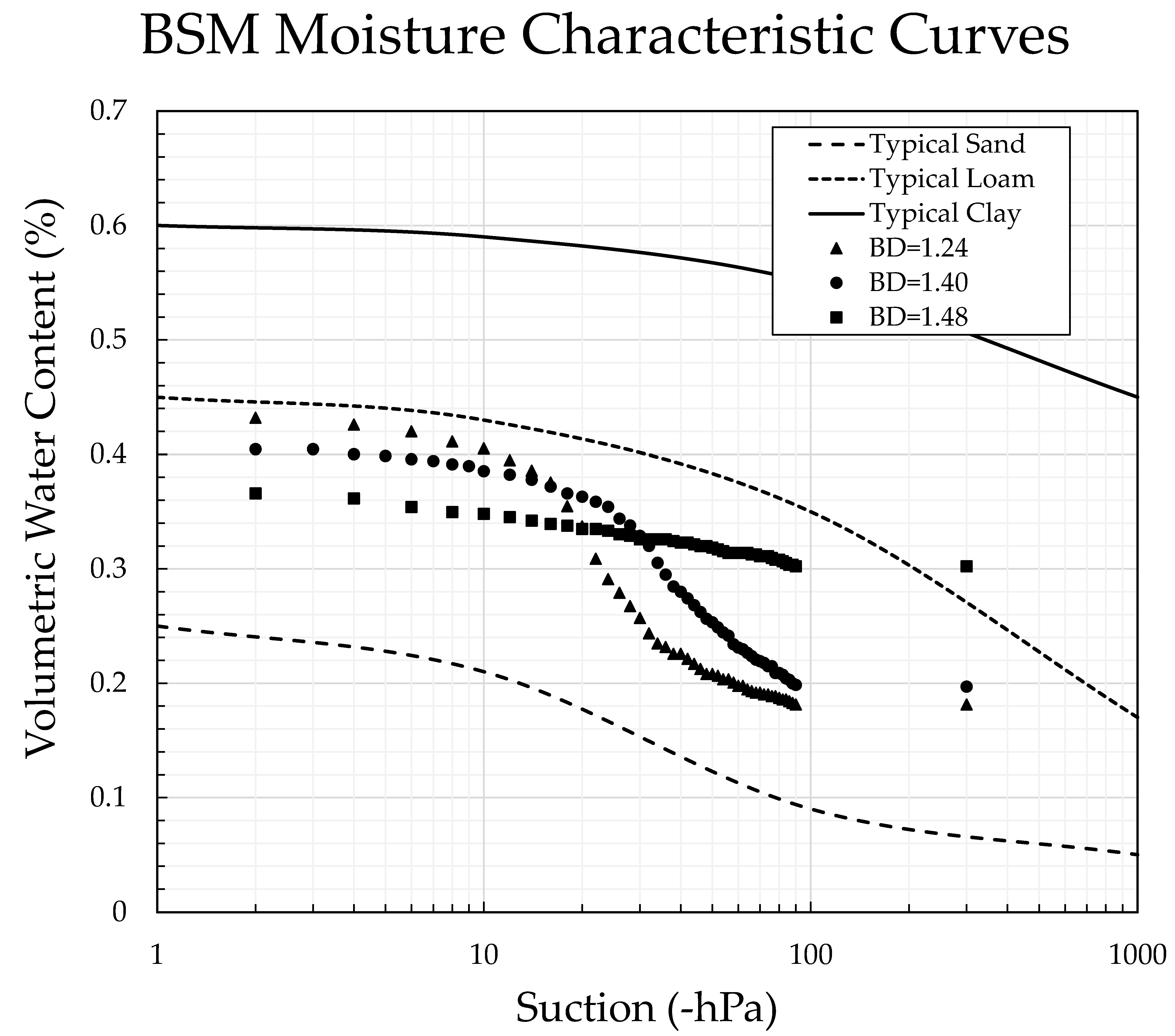
Soil moisture characteristic curves were developed for BSM meeting the target parameters as well as BSM at lower and higher bulk densities (Figure 3). At the target bulk density of 1.40 g cm−3, the saturated water content (porosity) was 41% with a field capacity of 20%. When the soil was compacted to 1.48 g cm−3, porosity dropped to 37% with a field capacity of 30%. In essentially un-compacted BSM, the porosity increased slightly to 43%, with a field capacity of 18%.
The difference between the volumetric water content at saturation and the volumetric water content at field capacity, approximately −100 to −300 hPa, approximates the amount of water that can be temporarily absorbed by the media during a rain event. An installation of uncompacted BSM would temporarily retain approximately 25% volumetric water content while a thoroughly boot compacted BSM would retain only about 6%. Conversely, the boot compacted soil would retain more water against infiltration during dry weather, which could help support plant growth. These data also reveal how the soil installation methods can dramatically alter the way water interacts with the BSM.
3.3. Mesocosm Installation Parameters
Before installation of the plant, mulch, and fungal elements, the saturated hydraulic conductivity was evaluated for each mesocosm over a two-month period using the falling head method [22]. Over the course of the Ksat testing, the bioretention soil in each drum received a total of 0.50 ± 0.03 m3 of municipal water, introduced from the bottom-up via a standpipe. The hydraulic conductivity of the installed mesocosms was approximately 50 ± 30 cm h−1, although the incremental development of a layer of fines (brought to the surface with the rising water table and escaping air bubbles) resulted in progressively decreasing saturated hydraulic conductivity measurements (Figure 4). These fines were collected, resuspended in water, and reincorporated into the soil after Ksat testing to ensure that all fines were appropriately represented in the BSM soil for the duration of the experiment.
3.4. Mesocosm Hydraulic Loading
The cumulative hydraulic loading preceding each water quality sampling event is summarized chronologically in Table 3. Each bioretention mesocosm received 6.9 m3 of stormwater over the 400-day loading period. This is a volume equivalent to 134 cm of rainfall on a 20:1 contributing area to treatment area ratio over 400 days, or roughly 10 cm per month as a yearly average.
3.5. Stormwater Sampling
The average influent water quality data is listed in Appendix A. The full water quality dataset is available as a CSV file in the supplementary materials. Note that for data analysis purposes, values that were below the detection limit of an analyte are assigned the value of ½ the detection limit concentration.
3.6. Statistical Analysis
3.6.1. Univariate Trends
Influent and effluent stormwater was sampled 5 times, roughly once every three months. During each sampling, influent and effluent concentrations of 65 distinct water quality parameters were collected. Each individual storm event was a ‘snapshot’ of performance at various points during the system’s operational lifetime (time and hydraulic loading). To reduce the dimensionality of the water quality parameter data to aid in analysis and interpretation, PAH congeners and metal species (for both total and dissolved metals) were grouped into their respective sum vectors. Ten water quality performance parameters are presented in Figure 5 and Figure 6. Data that met the required statistical assumptions are presented in Figure 5 as multiple linear regression models with 95% confidence intervals for water quality parameters and parameter groups as functions of time and biological amendment factor. All data is presented as concentration removed (positive values) or as concentration exported (negative values).
In Figure 5A,B both time and attribute type were significant predictors of the influent to effluent change in phosphorus concentration. The BSM in all mesocosms leached phosphorus throughout the 400-day study period, and the leaching rate was significantly correlated with time. Notably, the phosphorus leaching rate was significantly diminished in the mesocosms inoculated with the fungus. In Figure 5C, time was a highly significant predictor of the total metals movement, and the interaction of soil temperature and biological attribute was a nearly significant predictor of the influent to effluent change in total metals concentration (p = 0.0503). Total metals changed from net export to net retention across the study period.
Water quality parameters with nonlinear, heteroscedastic, autocorrelated, or non-normal data that could not be appropriately transformed for linear regression are presented as scatterplots with LOESS smoothing in Figure 6. LOESS smoothing is a computational approach based on fitting multiple localized nonparametric low order polynomials to the data and is intended to aid in graphical interpretation of data sets rather than as a rigorous statistical regression. Accordingly, parameter significance and goodness of fit statistics are not reported for these figures.
The overarching feature of the water chemistry is the substantial leaching of nutrients from the BSM over the 400-day study period. The media consistently exported total nitrogen (Figure 6B) and nitrate + nitrite (Figure 6D) over the study period, but exports of those parameters decreased over time and approached zero net exports by the third sampling event (245 days of operation). Removal of total and dissolved metals by the BSM mesocosms also followed an interesting pattern. During the first 200–250 days of operation the BSM exported total and dissolved metals (Figure 5C and Figure 6F). This timeframe corresponds with a clear conditioning period for the BSM as represented by total suspended sediment removal (Figure 6A). During the first 200–250 days, the incoming load of stormwater sediment was nearly equally matched by compost and sand sediments leaching from the BSM. When sediment exports from the BSM decreased after about 200 days, the shift to net sediment removal was accompanied by a net removal of total and dissolved metals.
While the sinusoidal effluent concentration patterns of ammonia and total PAHs (Figure 6C,E) suggests the possibility of a seasonal effect, a single year of data is not sufficient to define this type of relationship. Future work at this field site will monitor additional storm events until two years of water quality data have been collected.
The most notable result is the reduced export of ortho-phosphorus in the BSM mesocosms inoculated with Stropharia rugoso-annulata. For the first two sampling events (days 49 and 113), the average ortho-phosphorus export from the six fungal-inoculated mesocosms was 46% (460 ppb) and 26% (170 ppb) less than the uninoculated mesocosms, respectively. Post-hoc Tukey’s HSD 95% family-wise confidence intervals on the linear model reveal that over the entire 400-day study period, the paired ortho-phosphorus export differences from mesocosms with both plants and fungi were significantly less than the mesocosms with only soil (p < 0.01) and less than the mesocosms with only plants (p < 0.05). Similar but not statistically significant trends were apparent in the total phosphorus data. These reductions in phosphorus export diminished over time but persisted from the start of the study through approximately 6–12 months of operation.
The effect of fungi alone or plants alone compared to their corresponding controls did not yield statistically significant differences for either ortho- or total phosphorus when analyzed by regression over the 400-day study period (Figure 5A,B). However, when considered as independent events, one-way ANOVA with Tukey HSD post-hoc analysis illustrated a pronounced reduction in ortho-phosphorus export during the first sampling event (p < 0.05) in treatments that included fungi, with a similar reduction in total phosphorus during the first two sampling events (p < 0.1).
3.6.2. Multivariate Trends
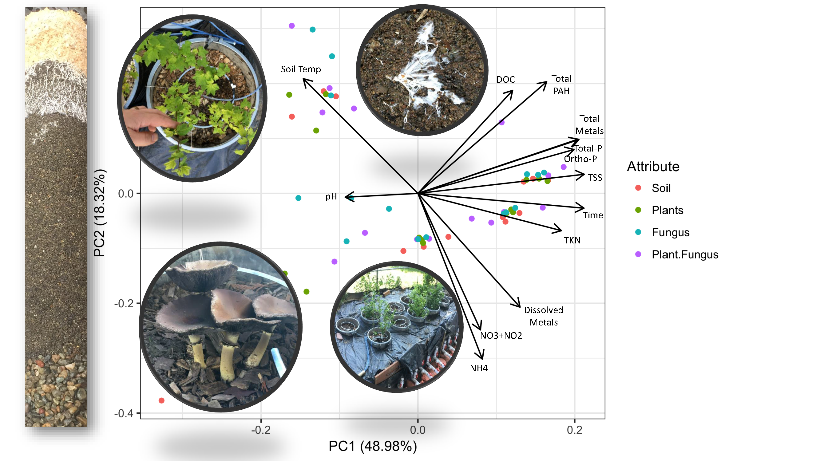
The high dimensionality (65 variables) and low number of observations (5 storms) presents some challenges when trying to identify main effects in complex, multivariate, repeated measures environmental data where covariation among response variables needs to be considered. Principal component analysis (PCA) and distance-based redundancy analysis are robust techniques for visualizing and accounting for these covariation effects.
The BSM effluent followed fairly clear covariation patterns that grouped as responses to the major physico-temporal factors governing most biological systems (e.g., temperature and time). The foremost effect was time, which in this experiment strongly covaried with hydraulic loading. The PCA plot clearly illustrates a positive time correlation for all water quality parameters (Figure 7). A particularly significant positive association with time is evident for ortho and total phosphorus, total metals, TSS, and total nitrogen (Figure 7)—all of which start as net exports and either export less with time, or cross into net retention, as with total metals and TSS (Figure 5C and Figure 6A).
This multivariate visualization also illustrates that soil temperature is negatively correlated with exports of soluble nitrogen species and dissolved metals. This is consistent with the general understanding that soil microbial activity increases at warm temperatures, which results in increased release of nutrients, particularly ammonium, during substrate digestion and produce nitrite/nitrate as the byproduct of aerobic oxidation. Increased temperature can also cause metals that were adsorbed to organic matter to become liberated during microbial digestion of the compost [6].
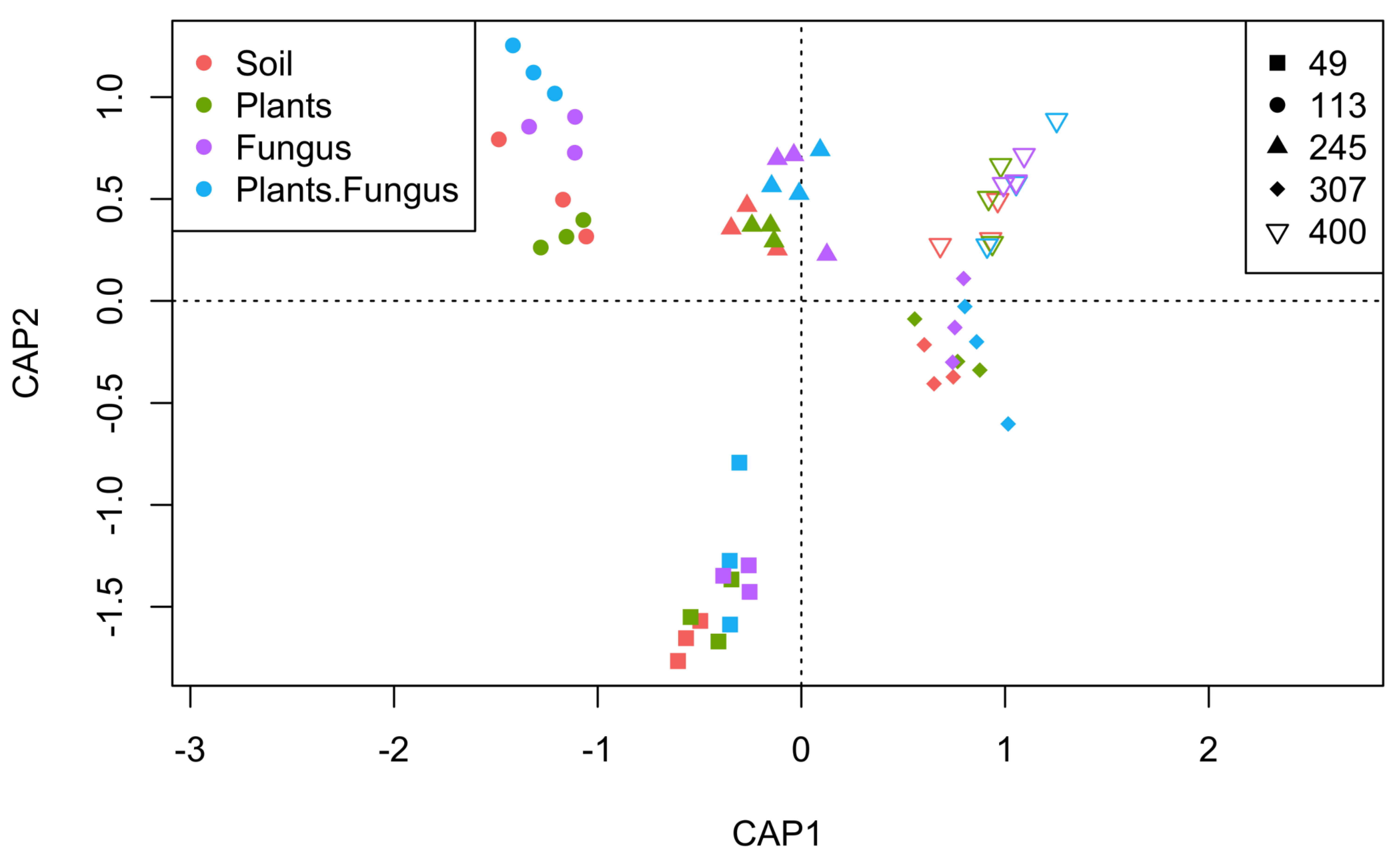
When the data is analysed from the ‘big picture’ perspective based on the combined water chemistry changes, it is clear that time and soil temperature change the water quality to a greater extent than the biological attributes. Figure 8 shows unconstrained distance-based redundancy analysis (dbRDA) illustrating each water quality sampling event for each treatment type as a single unique point where the Mahalanobis distance dissimilarity matrix defines the location of each point in multidimensional space and the bdRDA algorithm ordinates the points by metric scaling along time, soil temperature, biological amendment axes to the bivariate projection of minimum variance. The data clusters primarily according to sampling date (shapes) rather than by biological attribute (color).
4. Discussion
This study set out to test fungal and plant mediated effects on stormwater chemistry in replicated bioretention systems operating under field conditions for an extended period of time. While it is not appropriate to extrapolate to “all fungi” and “all plants” in bioretention systems, this study does provide some insight into the driving forces in porous media based biofiltration systems. While the biological elements of this model system provide many benefits including aesthetics, habitat, hydrology, and public engagement, the biological contributions to effluent water quality after 400 days of continuous operation were detectible, but relatively minor. Fundamental factors such as time and temperature were far more important to water quality in treated effluent. Time-dependent leaching of the compost-rich media dominated the trends in the effluent data, likely obscuring underlying plant and fungal contributions.
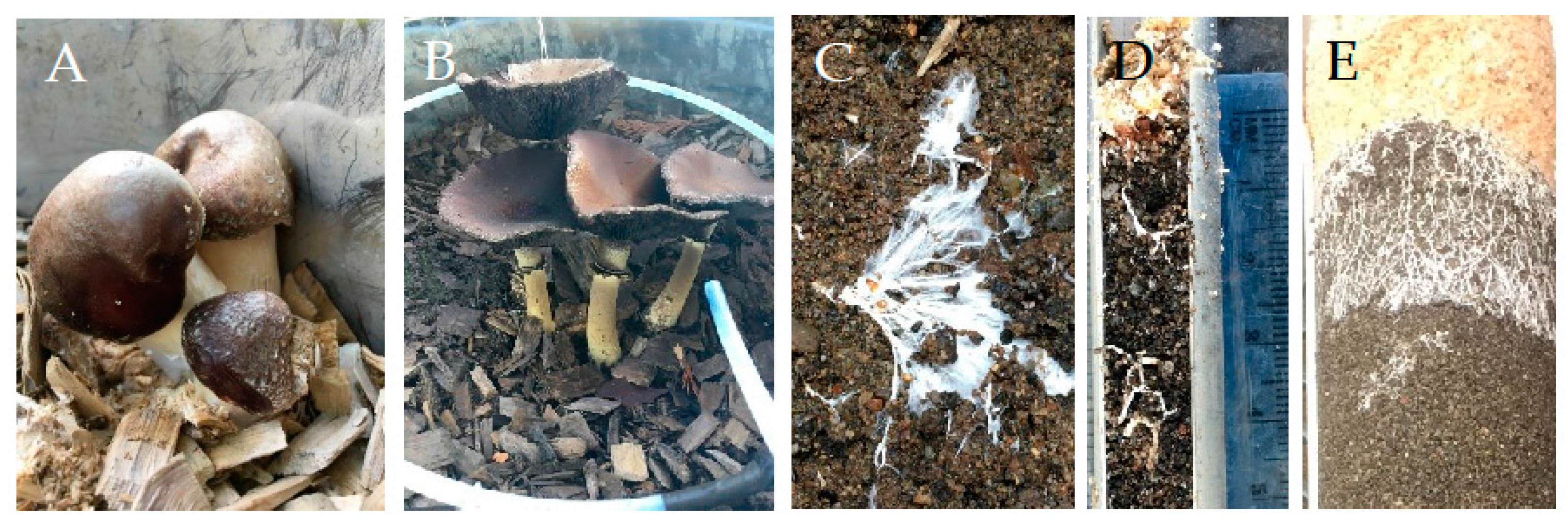
Despite the considerable leaching from the BSM, ortho-phosphorus and total phosphorus exports were reduced in treatments with both plants and fungi compared to soil alone, and the presence of fungi reduced ortho-phosphorus export when compared with the plant only mesocosms. The addition of the Stropharia rugoso-annulata fungus to the wood mulch layer slowed the release of phosphorus from this nutrient-rich media, particularly when co-occurring with plants. This edible mushroom-forming species is classified as a forest litter decomposer [32], and the mycelium of this soil-wood interfacing organism clearly grew into both the BSM and the wood chip mulch (Figure 9). Translocation of phosphorus by soil fungi is a well-documented biological process, particularly for mycorrhizal fungi [33], but nutrient translocation to aid in the breakdown of high carbon:nitrogen and high carbon:phosphorus wood is also an established but less well known phenomenon in saprophytic fungi [34].
An alternative hypothesis is that the phosphorus used by the fungi came from the alder wood chip mulch rather than the BSM, and the increased phosphorus exports from the mesocosm without inoculated mulch came from the wood chip leachate that was not absorbed by the fungus. However, this is not a sufficient explanation for the reduction in phosphorus exports that were observed. Red alder heartwood (Alnus rubra), such as that used in this study, contains approximately 0.01% organic phosphorus by dry mass [35]. Even if 100% of the phosphorus in the alder wood chips had been available as ortho-phosphate (an extreme assumption), it would only amount to 100 mg kg−1, or roughly 500 mg per mesocosm. Considering the measured ortho-phosphate concentration in the BSM (135 mg kg−1) and the mass (145 kg), the maximum possible wood chip contribution to the pool of ortho-phosphate available in the bioretention mesocosms is roughly 2.5%.
Another alternative hypothesis is that mycelium growth into the BSM helped stabilize TSS export, and the reduction in TSS would predict the reduction in ortho-phosphorus leachate. This hypothesis is not supported by the data because no significant differences in TSS leachate were observed between the fungal-inoculated mesocosms and those that received only the wood mulch during the period when ortho-phosphate differences were apparent.
The observation of extensive growth of mycelium into the soil and the documented ability of saprophytic fungi to translocate and accumulate phosphorus from their environment [34], suggests that translocation processes underlie some of the observed reduction in phosphorus exports, although these hypotheses were not explicitly tested. This presents a noteworthy opportunity to explore the use of cultivated fungi for stabilizing and mineralizing soil phosphorus to reduce loses from leaching or erosion in bioretention systems and other engineered environments.
This study also highlights how easily the BSM installation process can dramatically alter the physical and hydrologic performance of the media. The BSM compacted to 1.48 g cm−3—which represents a bulk density roughly equivalent to boot packing the BSM every 8 cm during installation—had a field capacity of roughly 30% but a lower porosity, while the uncompacted soil had a field capacity of was around 20% and considerably more porosity. This suggests that bioretention installations where attenuation of peak flow is most important may benefit from less compacted soil, while bioretention installations that need to maintain plant available water during extended dry periods may benefit from a more compacted soil.
The hydraulic conductivity of uncompacted and compacted soil was correspondingly affected by bulk density, with a five to ten-fold change from roughly 100 cm h−1 to 10–20 cm h−1. The magnitude of these physical differences and the dramatic effect they can have on water retention time and soil pore water mediated nutrient uptake should not be overlooked by environmental engineers seeking to explore plant or bioretention media composition changes. Failure to adequately control for bulk density and hydraulic conductivity can seriously compromise design optimization results, especially when media components are proportioned by volume [4].
We observed fines mobilizing to the surface of the BSM after saturating the bioretention installations from the bottom for hydraulic conductivity testing. The thick layer of fines decreased saturated hydraulic conductivity over the course of testing. This result is congruent with the findings of a 2007 investigation of the possible mechanisms responsible for hydraulic failure of bioretention systems in Australia [36]. The mobility of fines in bioretention installations using the “60:40” default soil mix installed per Washington State guidelines suggests a need to reconsider the soil specifications.
In addition to possible problems with infiltration caused by mobilization and agglomeration of fines at hydraulic transition layers, the mobilized fine particles amounted to at least 1.0% of the total soil mass, 2.2% of the total compost mass, 6.8% of the total nitrogen, and 4.6% of the plant-available phosphorus. For hydrologic perspective, this soil mix compacted to a bulk density of 1.41 ± 0.04 g cm−3 per SWMMWW specifications had a porosity of approximately 0.45 cm3 cm−3, assuming a sand particle density of 2.65 g cm−3 and a compost particle density of 2.60 g cm−3 [37]. The 9.6 pore volume equivalents of water used in the Ksat testing which mobilized the fine particles had a soil water equivalent of 9.7 ± 0.7 cm of rainfall at a 20:1 (5%) impervious area to treatment area ratio. This is equivalent to a conditioning period of around 2–6 weeks during the western Washington rainy season (Oct–Mar).
Taken together, these data corroborate field studies that have documented dissolved and particulate nutrient and metal export from bioretention systems containing high compost fractions, however the inclusion of plants, and especially fungi, reduced phosphorus exports.
The data reported here were collected as part of an ongoing study that will evaluate the performance of this field system for a second year. Additional research perspectives will include toxicological performance assays in a zebrafish (Danio rerio) model, analysis of changes in soil volumetric water content and Ksat across treatments over time, and analysis of treatment performance on additional anthropogenic toxicants including polychlorinated biphenyls. Destructive sampling of plant and microbial biomass and chemical testing of soil strata after the two-year sampling is complete will add additional context and insight to the results reported thus far.
Supplementary Materials
The following are available online at https://www.mdpi.com/2073-4441/10/9/1226/s1.
Author Contributions
Conceptualization, A.T. and J.M.; Data curation, A.T.; Formal analysis, A.T.; Funding acquisition, A.T., J.D. and J.M.; Investigation, A.T., J.W., E.M., K.K. and J.C.; Methodology, A.T. and J.M.; Project administration, J.D. and J.M.; Supervision, J.M.; Visualization, A.T.; Writing—original draft, A.T.; Writing—review & editing, J.D. and J.M.
Funding
This research was funded by the Stormwater Action Monitoring program administered by the Washington State Department of Ecology under contract number [C1600135] and the APC was funded by Washington State University.
Acknowledgments
This work would not have been possible without the help of many dedicated and hardworking assistants including Cailin Mackenzie, Chelsea Mitchell, Jasmine Pratt, Benjamin Leonard, among many other staff at the WSU Puyallup Research and Extension Center. We would also like to thank Ani Jayakaran and Joan Wu, for their methodological and statistical insights as well as Markus Flury for his help with the soil physics experiments. Mountlake Terrace High School seniors Maxwell Ledeig and Vesta Baumgartner are acknowledged for their engagement in building and testing a microcosm analog and for their accomplishments leading to a first-place regional science fair competition in environmental engineering. Washington State Department of Transportation, Carla Milesi, and Dylan Ahearn provided essential access to the test facility. We would also like to thank Heather Kibbey, Brandi Lubliner, and the other guiding members of the Stormwater Action Monitoring collaboration for their foresight and support of this research. Finally, we thank the anonymous peer reviewers for their very thorough, critical, and helpful review.
Conflicts of Interest
A.T. declares a perceived but not material conflict of interest because of his position as a staff engineer for Fungi Perfecti, LLC—a supplier of mushroom-based dietary supplements and mushroom cultivation tools and equipment. While Fungi Perfecti does supply mushroom spawn of the type used in this study, A.T. receives no monetary or other compensation resulting from this research. The other authors declare no conflict of interest. The founding sponsors had no role in the design of the study; in the collection, analyses, or interpretation of data; in the writing of the manuscript, and in the decision to publish the results.
Disclaimer
The findings and conclusions in this article are those of the authors and do not necessarily represent the views of the affiliated organizations.
Appendix A
| Parameter Class | Parameters | Mean | SD | Detection Limit |
| Total Metals | Aluminum (μg/L) | 876 | 570 | 0.5 |
| Antimony (μg/L) | 7.71 | 11.4 | 0.2 | |
| Arsenic (μg/L) | 3.25 | 2.99 | 0.02 | |
| Barium (μg/L) | 68.5 | 19.6 | 0.1 | |
| Copper (μg/L) | 40.5 | 9.15 | 0.1 | |
| Lead (μg/L) | 10.9 | 6.90 | 0.05 | |
| Manganese (μg/L) | 77.0 | 30.1 | 0.03 | |
| Molybdenum (μg/L) | 7.20 | 13.0 | 0.05 | |
| Nickel (μg/L) | 6.62 | 9.56 | 0.05 | |
| Selenium (μg/L) | 1.49 | 2.05 | 0.25 | |
| Silver (μg/L) | 3.62 | 3.89 | 0.05 | |
| Thallium (μg/L) | 0.408 | 0.559 | 0.01 | |
| Vanadium (μg/L) | 2.45 | 1.36 | 0.02 | |
| Zinc (μg/L) | 123 | 51.0 | 0.5 | |
| Dissolved Metals | Aluminum (μg/L) | 53.6 | 61.1 | 0.5 |
| Antimony (μg/L) | 3.02 | 0.936 | 0.2 | |
| Arsenic (μg/L) | 1.33 | 0.520 | 0.02 | |
| Barium (μg/L) | 40.1 | 9.90 | 0.25 | |
| Copper (μg/L) | 16.7 | 5.37 | 0.1 | |
| Lead (μg/L) | 0.805 | 1.33 | 0.05 | |
| Manganese (μg/L) | 13.8 | 16.4 | 0.03 | |
| Molybdenum (μg/L) | 3.5 | 1.81 | 0.05 | |
| Nickel (μg/L) | 2.04 | 0.773 | 0.05 | |
| Selenium (μg/L) | 0.168 | 0.093 | 0.25 | |
| Silver (μg/L) | 0.200 | 0.099 | 0.05 | |
| Thallium (μg/L) | <DL | <DL | 0.01 | |
| Vanadium (μg/L) | 1.02 | 0.390 | 0.02 | |
| Zinc (μg/L) | 43.6 | 26.9 | 0.5 | |
| Nutrients | NH4 (mg/L) | 0.257 | 0.096 | 0.005 |
| TKN (mg/L) | 1.28 | 0.179 | 0.1 | |
| NO3/NO2 (mg/L) | 0.663 | 0.333 | 0.01 | |
| Ortho-Phosphorus (mg/L) | 0.027 | 0.030 | 0.005 | |
| Total Phosphorus (mg/L) | 0.097 | 0.022 | 0.005 | |
| Conventionals, Microbiology | Alkalinity (mg/L) | 38.4 | 15.4 | 1 |
| TSS (mg/L) | 34.3 | 19.4 | 1 | |
| pH (-log[H3O]) | 6.76 | 0.505 | 0.1 | |
| BOD (mg/L) | 17.9 | 11.6 | 2 | |
| DOC (mg/L) | 7.86 | 5.24 | 0.5 | |
| TOC (mg/L) | 14.69 | 10.3 | 0.2 | |
| E. coli (MPN/100 mL) | 3090 | 1640 | 1 | |
| Fecal coliform (CFU/100 mL) | 2960 | 2060 | 1 | |
| PAH Congeners | Naphthalene (μg/L) | 0.023 | 0.014 | 0.012 |
| 1-Methylnaphthalene (μg/L) | 0.011 | 0.007 | 0.012 | |
| 2-Methylnaphthalene (μg/L) | 0.011 | 0.005 | 0.012 | |
| Acenaphthylene (μg/L) | 0.011 | 0.010 | 0.012 | |
| Acenaphthene (μg/L) | 0.007 | 0.002 | 0.012 | |
| Dibenzofuran (μg/L) | 0.007 | 0.002 | 0.012 | |
| Fluorene (μg/L) | 0.007 | 0.002 | 0.012 | |
| Phenanthrene (μg/L) | 0.022 | 0.025 | 0.012 | |
| Anthracene (μg/L) | 0.033 | 0.036 | 0.012 | |
| Fluoranthene (μg/L) | 0.030 | 0.034 | 0.012 | |
| Pyrene (μg/L) | 0.046 | 0.051 | 0.012 | |
| Benzo(a)anthracene (μg/L) | 0.047 | 0.048 | 0.012 | |
| Chrysene (μg/L) | 0.080 | 0.083 | 0.012 | |
| Benzo(a)pyrene (μg/L) | 0.042 | 0.026 | 0.012 | |
| Indeno(1,2,3-cd)pyrene (μg/L) | 0.029 | 0.029 | 0.012 | |
| Dibenzo(a,h)anthracene (μg/L) | 0.027 | 0.043 | 0.012 | |
| Benzo(g,h,i)perylene (μg/L) | 0.034 | 0.030 | 0.012 | |
| Perylene (μg/L) | 0.044 | 0.036 | 0.012 |
References
- National Academy of Sciences. Urban Stormwater Management in the United States; The National Academies Press: Washington, DC, USA, 2008; Volume 610. [Google Scholar] [CrossRef]
- Davis, A.P.; Hunt, W.F.; Traver, R.G.; Clar, M. Bioretention Technology: Overview of Current Practice and Future Needs. J. Environ. Eng. 2009, 135, 109–117. [Google Scholar] [CrossRef]
- Herrera Environmental Consultants. Pacific Northwest Bioretention Performance Study Synthesis Report, Prepared for the City of Redmond. Available online: http://www.wastormwatercenter.org/news/?id=1269 (accessed on 7 March 2017).
- Herrera Environmental Consultants. Analysis of Bioretention Soil Media for Improved Nitrogen, Phosphorus, and Copper Retention, Prepared for Kitsap County Public Works. Available online: www.wastormwatercenter.org/file_viewer.php?id=3491 (accessed on 24 February 2017).
- Lefevre, G.H.; Paus, K.H.; Natarajan, P.; Gulliver, J.S.; Novak, P.J.; Hozalski, R.M. Review of dissolved pollutants in urban storm water and their removal and fate in bioretention cells. J. Environ. Eng. 2015, 141, 04014050. [Google Scholar] [CrossRef]
- Cording, A. Evaluating Stormwater Pollutant Removal Mechanisms by Bioretention in the Context of Climate Change. Ph.D. Thesis, University of Vermont, Burlington Vermont, VT, USA, 2016; p. 541. [Google Scholar]
- Washington State Department of Ecology. Stormwater Management Manual for Western Washington. Publication 14-10-055. Available online: https://ecology.wa.gov/Regulations-Permits/Guidance-technical-assistance/Stormwater-permittee-guidance-resources/Stormwater-manuals (accessed on 24 March 2014).
- Mullane, J.; Flury, M.; Iqbal, H.; Shi, Z. Intermittent rainstorms cause pulses of nitrogen, phosphorus, and copper in leachate from compost in bioretention systems. Sci. Total Environ. 2015, 537, 294–303. [Google Scholar] [CrossRef] [PubMed] [Green Version]
- Herrera Environmental Consultants. Pollutant Export from Bioretention Soil Mix, 185th Ave NE, Redmond, WA, USA. Available online: http://www.redmond.gov/Environment/StormwaterUtility/LID/185ave/ (accessed on 5 May 2016).
- Paus, K.H.; Morgan, J.; Gulliver, J.S.; Hozalski, R.M. Effects of bioretention media compost volume fraction on toxic metals removal, hydraulic conductivity, and phosphorus release. J. Environ. Eng. 2014, 140. [Google Scholar] [CrossRef]
- Howie, D.C. Memo: Focus on Bioretention Soil Media. Washington State Department of Ecology Water Quality Program. Publication 13-10-017. Available online: https://fortress.wa.gov/ecy/paris/ DownloadDocument.aspx?id=204469 (accessed on 16 March 2018).
- McIntyre, J.K.; Lundin, J.I.; Cameron, J.R.; Scholz, N.L. Interspecies variation in the susceptibility of adult Pacific salmon to toxic urban stormwater runoff. Environ. Pollut. 2018, 238, 196–203. [Google Scholar] [CrossRef] [PubMed]
- McIntyre, J.K.; Davis, J.; Hinman, C.; Macneale, K.H.; Anulacion, B.F.; Scholz, N.L.; Stark, J.D. Soil bioretention protects juvenile salmon and their prey from the toxic impacts of urban stormwater runoff. Chemosphere 2015, 132, 213–219. [Google Scholar] [CrossRef] [PubMed]
- Palmer, E.T.; Poor, C.J.; Hinman, C.; Stark, J.D. Nitrate and phosphate removal through enhanced bioretention media: Mesocosm study. Water Environ. Res. 2013, 85, 823. [Google Scholar] [CrossRef] [PubMed]
- Bratieres, K.; Fletcher, T.; Deletic, A.; Zinger, Y. Nutrient and sediment removal by stormwater biofilters: A large-scale design optimization study. Water Res. 2008, 42, 3930–3940. [Google Scholar] [CrossRef] [PubMed]
- Thomas, S.A.; Aston, L.M.; Woodruff, D.L.; Cullinan, V.I. Field Demonstration of Mycoremediation for Removal of Fecal Coliform Bacteria and Nutrients in the Dungeness Watershed, Washington; Final Report PNWD-4054-1; Pacific Northwest National Laboratory: Richland, WA, USA, 2009.
- Taylor, A.; Flatt, A.; Beutel, M.; Wolff, M.; Brownson, K.; Stamets, P. Removal of Escherichia coli from Synthetic Stormwater Using Mycofiltration. Ecol. Eng. 2015, 78, 79–86. [Google Scholar] [CrossRef]
- Steffen, K.T.; Schubert, S.; Tuomela, M.; Hatakka, A.; Hofrichter, M. Enhancement of bioconversion of high-molecular mass polycyclic aromatic hydrocarbons in contaminated non-sterile soil by litter-decomposing fungi. Biodegradation 2007, 18, 359–369. [Google Scholar] [CrossRef] [PubMed]
- Mohapatra, D.; Rath, S.K.; Mohapatra, P.K. Bioremediation of Insecticides by White-Rot Fungi and Its Environmental Relevance. In Mycoremediation and Environmental Sustainability. Fungal Biology; Prasad, R., Ed.; Springer: Cham, Switzerland, 2018. [Google Scholar] [CrossRef]
- ASTMD2216-10. ASTM D2216-10-Standard Test Methods for Laboratory Determination of Water (Moisture) Content of Soil and Rock by Mass; ASTM International: West Conshohocken, PA, USA, November 1988; pp. 1–7. [Google Scholar] [CrossRef]
- ASTMD1557-12. Standard Test Methods for Laboratory Compaction Characteristics of Soil Using Modified Effort; ASTM International: West Conshohocken, PA, USA, 2012. [Google Scholar] [CrossRef]
- Flury, M. Soil Physics Laboratory Manual. Department of Crop and Soil Sciences; Washington State University: Pullman, WA, USA, 2015. [Google Scholar]
- Washington State Department of Transportation. Traffic Data Geoportal. Available online: http://www.wsdot.wa.gov/mapsdata/tools/trafficplanningtrends.htm (accessed on May 9 2018).
- R Core Team. R: A Language and Environment for Statistical Computing; Version 3.4.0.; R Foundation for Statistical Computing: Vienna, Austria, 2017; Available online: https://www.R-project.org (accessed on 16 March 2018).
- RStudio Team. RStudio: Integrated Development for R. Version 1.0.143; RStudio, Inc.: Boston, MA, USA, 2016; Available online: http://www.rstudio.com (accessed on 16 March 2018).
- Wickham, H.; Francois, R.; Henry, L.; Müller, K.; Wickham, H. Dplyr: A Grammar of Data Manipulation. Available online: https://CRAN.R-project.org/package=dplyr (accessed on 16 March 2018).
- Fox, J.; Weisberg, S. An {R} Companion to Applied Regression, 2nd ed.; Sage: Thousand Oaks, CA, USA; Available online: http://socserv.socsci.mcmaster.ca/jfox/Books?Companion (accessed on 16 March 2018).
- Korkmaz, S.; Goksuluk, D.; Zararsiz, G. MVN: An R Package for Assessing Multivariate Normality. R J. 2014, 6, 151–162. [Google Scholar]
- Revelle, W. Psych: Procedures for Personality and Psychological Research; Northwestern University: Evanston, IL, USA; Available online: https://CRAN.R-project.org/package=psych (accessed on 16 March 2018).
- Oksanen, J.; Blanchet, F.G.; Friendly, M.; Kindt, R.; Legendre, P.; McGlinn, D.; Minchin, P.R.; O’Hara, R.B.; Simpson, G.L.; Solymos, P.; et al. Vegan: Community Ecology Package. Available online: https://CRAN.R-project.org/package=vegan (accessed on 16 March 2018).
- Sullivan, D.M.; Stevens, R.G. Agricultural Phosphorus Management Using the Oregon/Washington Phosphorus Indexes; Oregon State University Extension Service. Publication EM 8848-E.; Oregon State University: Corvallis, OR, USA, 2003. [Google Scholar]
- Aurora, D. Mushrooms Demystified: A Comprehensive Guide to the Fleshy Fungi, 2nd ed.; Ten Speed Press: Berkeley, CA, USA, 1986. [Google Scholar]
- Deacon, J. Fungal Biology, 4th ed.; Blackwell Publishing: Malden, MA, USA, 2006. [Google Scholar]
- Dighton, J. Fungi in Ecosystem Processes, 2nd ed.; CRC Press: Boca Raton, FL, USA, 2016. [Google Scholar]
- Diez, J.; Elosegi, A.; Chauvet, E.; Pozo, J. Breakdown of wood in the Agüera stream. Freshw. Biol. 2002, 47, 2205–2215. [Google Scholar] [CrossRef]
- Siriwardene, N.R.; Deletic, A.; Fletcher, T.D. Clogging of stormwater gravel infiltration systems and filters: Insights from a laboratory study. Water Res. 2007, 41, 1433–1440. [Google Scholar] [CrossRef] [PubMed]
- Weindorf, D.C.; Wittie, R. Determining Particle Density in Dairy Manure Compost. Tex. J. Agric. Nat. Resour. 2003, 16, 60–63. [Google Scholar]
Figure 1.
Bioretention mesocosms in an urban watershed in Seattle, WA.

Figure 2.
Bench-scale range finding experiments to determine the target bulk density for the field mesocosms. (A) Plot of bulk density as a function of water content. The triangular datum is a suspected outlier due to separation of the sand and compost while filling test apparatus. (B) Plot of saturated hydraulic conductivity as a function of soil bulk density.

Figure 3.
Moisture retention curves for the BSM expressed as the suction (–pressure) required to extract water from the bioretention soil matrix. Different levels of soil compaction are represented as bulk density “BD” in g cm−3 in the figure legend. The BSM compacted to 1.48 g cm−3 had a markedly higher field capacity than the 1.40 g cm−3 BSM, which more closely followed the characteristic curve of the uncompacted BSM (1.24 g cm−3).

Figure 4.
(left) Data represent the mean Ksat value ± standard deviation for n = 12 bioretention cells (trials 1–3); n = 10–12 bioretention cells (trials 4–8); and n = 8 bioretention cells (trial 9). Triangles represent trials at bulk density = 1.25 ± 0.04 g cm−3, circles represent trials at bulk density = 1.41 ± 0.04 g cm−3. (A) A thin layer of fines rose through the bioretention soil with the rising water table during Ksat testing. (B) The thickness of the layer of fines increased up to approximately 0.5 cm over the course of nine Ksat tests over eight weeks.

Figure 5.
Multiple linear regression models with 95% confidence intervals for ortho-phosphorus (A), total phosphorus (B) and total metals (C) as functions of time and biological amendment factor. In all subfigures the * symbol indicates statistical significance: * p < 0.05, ** p < 0.01, *** p < 0.001. The asterisk next to each panel letter indicates the significance of the regression model. The marginal significance of the individual model variables are indicated for time and biological attributes.

Figure 6.
Non-parametric Locally Weighted Scatterplot Smoothing (LOESS) for total suspended sediment (A), total Kjeldahl nitrogen (B), ammonia + ammonium (C), nitrate + nitrite (D), total polycyclic aromatic hydrocarbons (E) and total dissolved metals (F) as functions of time with each biological amendment factor presented independently. All data are presented as concentration removed (positive values) or as concentration exported (negative values).

Figure 7.
Principle component analysis biplot describing 67% of water quality parameter variance. The observations (colored by attribute) and factor loadings of ten water quality response and three continuous explanatory variables tend to group by time, soil temperature, pH, and TSS.
Figure 7.
Principle component analysis biplot describing 67% of water quality parameter variance. The observations (colored by attribute) and factor loadings of ten water quality response and three continuous explanatory variables tend to group by time, soil temperature, pH, and TSS.

Figure 8.
Unconstrained distance-based redundancy analysis (dbRDA) biplot illustrating that the water quality data clusters primarily according to sampling date (shapes) rather than by biological attribute (color). The distance between data points is proportional to their dissimilarity.
Figure 8.
Unconstrained distance-based redundancy analysis (dbRDA) biplot illustrating that the water quality data clusters primarily according to sampling date (shapes) rather than by biological attribute (color). The distance between data points is proportional to their dissimilarity.

Figure 9.
Growth of Stropharia rugoso-annulata. (A,B) Fruiting bodies emerged periodically over the study, confirming growth of the intended organism and verifying that the environmental conditions in the bioretention cell were conducive to its growth. (C) Mycelium growing on the BSM-mulch interface. (D,E) Root-like rhizomorphic mycelium extending down into the BSM both in the field as illustrated by the soil core (D) and in bench scale microcosms (E) made with the same materials (microcosm construction and photo credit: Maxwell Ledeig and Vesta Baumgartner; Mountlake Terrace High School).


Table 1.
Metal concentrations (mg kg−1) of compost and sand used in BSM.
| Value | Al | Sb | As | Ba | Cd | Cr | Co | Cu | Pb | Mg | Ni | Va | Zn |
|---|---|---|---|---|---|---|---|---|---|---|---|---|---|
| Compost | |||||||||||||
| Mean | 5540 | 0.703 | 7.95 | 88.3 | 0.449 | 16.6 | 5.10 | 39.9 | 35.7 | 264 | 11.3 | 15.3 | 148 |
| St. Dev | 581.3 | 0.465 | 4.64 | 6.8 | 0.054 | 1.7 | 2.20 | 8.2 | 7.1 | 81 | 1.1 | 2.1 | 35 |
| RSD (%) 1 | 9.5 | 1.5 | 1.7 | 13.1 | 8.3 | 9.9 | 2.3 | 4.9 | 5.1 | 3.3 | 10.5 | 7.3 | 4.2 |
| D.L. 1 | 0.86 | 0.086 | 0.052 | 0.086 | 0.086 | 0.086 | 0.86 | 0.086 | 0.086 | 0.086 | 0.086 | 0.086 | 0.17 |
| Sand | |||||||||||||
| Mean | 8220 | -- | 0.53 | 20.9 | 0.051 | 14.3 | 5.89 | 16.0 | 1.2 | 183 | 17.4 | 26.6 | 17.4 |
| St. Dev | 632.2 | -- | 0.16 | 3.7 | 0.021 | 4.7 | 0.14 | 1.3 | 0.3 | 15 | 3.3 | 5.6 | 1 |
| RSD (%) 1 | 13.0 | -- | 3.3 | 5.6 | 2.4 | 3.0 | 41.5 | 12.0 | 3.9 | 12.0 | 5.3 | 4.8 | 19.2 |
| D.L. 1 | 0.43 | 0.043 | 0.025 | 0.043 | 0.043 | 0.086 | 0.86 | 0.086 | 0.086 | 0.086 | 0.086 | 0.086 | 0.17 |
1 RSD = relative standard deviation (St. Dev/Mean); D.L. = detection limit.
Table 2.
Chemical characteristics of BSM.
| Value | Total C (%) | Total N (%) | Total P (mg kg−1) | NH4-N (mg kg−1) | NO3-N (mg kg−1) | Olsen P (mg kg−1) | CEC (meq 100 g−1) | pH -log [H3O+] |
|---|---|---|---|---|---|---|---|---|
| Mean | 1.8 | 0.14 | 678 | 1.9 | 52 | 29 | 1.8 | 7.1 |
| St. Dev. | 0.2 | 0.01 | 44 | 0.3 | 10 | 4 | 0.4 | 0.1 |
| RSD (%) 1 | 13 | 5.6 | 6.5 | 13 | 20 | 13 | 4.6 | 0.8 |
| D.L. 1 | 0.01 | 0.02 | 4.3 | 0.7 | 0.8 | 0.9 | 0.1 | 0.1 |
1 RSD = relative standard deviation; D.L. = detection limit.
Table 3.
Summary of cumulative hydraulic loading by sampling date *
| Date | Days in Operation | Total Vol. TTD 1 (m3) | Total Vol. TTD 1 (PVE2) | Total Vol. TTD 1 (cm) | Equiv. Precip. TTD 1 (cm at 20:1 rate) |
|---|---|---|---|---|---|
| 5 April 2017 | 49 | 1.2 | 26.3 | 467 | 23 |
| 8 June 2017 | 113 | 1.9 | 42.8 | 760 | 38 |
| 18 October 2017 | 245 | 2.4 | 52.1 | 924 | 46 |
| 19 December 2017 | 307 | 3.9 | 85.3 | 1512 | 76 |
| 22 March 2018 | 400 | 6.9 | 151 | 2680 | 134 |
* The loading rate during each event was constant at 0.12 L min−1, 1 TTD: Treated-to-Date. 2 PVE: Soil Pore Volume Equivalent.
© 2018 by the authors. Licensee MDPI, Basel, Switzerland. This article is an open access article distributed under the terms and conditions of the Creative Commons Attribution (CC BY) license (http://creativecommons.org/licenses/by/4.0/).
Share and Cite
MDPI and ACS Style
Taylor, A.; Wetzel, J.; Mudrock, E.; King, K.; Cameron, J.; Davis, J.; McIntyre, J. Engineering Analysis of Plant and Fungal Contributions to Bioretention Performance. Water 2018, 10, 1226. https://doi.org/10.3390/w10091226
AMA Style
Taylor A, Wetzel J, Mudrock E, King K, Cameron J, Davis J, McIntyre J. Engineering Analysis of Plant and Fungal Contributions to Bioretention Performance. Water. 2018; 10(9):1226. https://doi.org/10.3390/w10091226
Chicago/Turabian StyleTaylor, Alex, Jill Wetzel, Emma Mudrock, Kennith King, James Cameron, Jay Davis, and Jenifer McIntyre. 2018. "Engineering Analysis of Plant and Fungal Contributions to Bioretention Performance" Water 10, no. 9: 1226. https://doi.org/10.3390/w10091226
Note that from the first issue of 2016, this journal uses article numbers instead of page numbers. See further details here.